Water Vapor on Betelgeuse as Revealed by TEXES High-Resolution $12\,\mu\mathrm{m}$ Spectra

Abstract

The outer atmosphere of the M supergiant Betelgeuse is puzzling. Published observations of different kinds have shed light on different aspects of the atmosphere, but no unified picture has emerged. They have shown, for example, evidence of a water envelope (MOLsphere) that in some studies is found to be optically thick in the mid-infrared. In this paper, we present high-resolution, mid-infrared spectra of Betelgeuse recorded with the TEXES spectrograph. The spectra clearly show absorption features of water vapor and OH. We show that a spectrum based on a spherical, hydrostatic model photosphere with $T_{\mathrm{eff}}=3600$ K, an effective temperature often assumed for Betelgeuse, fails to model the observed lines. Furthermore, we show that published MOLspheres scenarios are unable to explain our data. However, we are able to model the observed spectrum reasonably well by adopting a cooler outer photospheric structure corresponding to $T_{\mathrm{mod}}=3250$ K. The success of this model may indicate the observed mid-infrared lines are formed in cool photospheric surface regions. Given the uncertainties of the temperature structure and the likely presence of inhomogeneities, we cannot rule out the possibility that our spectrum could be mostly photospheric, albeit non-classical. Our data put new, strong constraints on atmospheric models of Betelgeuse and we conclude that continued investigation requires consideration of non-classical model photospheres as well as possible effects of a MOLsphere. We show that the mid-infrared water-vapor features have great diagnostic value for the environments of K and M (super-) giant star atmospheres.

1 INTRODUCTION

The issue of water vapor in the atmosphere of Betelgeuse ($\alpha$ Orionis; M1-2 Ia-Iab; Keenan & McNeil, 1989) has a 40-year history. A detection was first proposed in 1964 by Woolf et al. (1964), but this was overlooked until it was confirmed by Tsuji (2000b) through reanalysis of the original data. Betelgeuse has been used as a water-free reference source in the near-infrared, see for example Hinkle & Barnes (1979). Jennings & Sada (1998) were the first, to our knowledge, to have identified individual rotational lines of water vapor in $R\approx 10,000$ spectra of Betelgeuse. They modeled their observations with a plane-parallel, isothermal layer close to the location of the onset of the chromospheric temperature rise. Tsuji (2000b) interpreted the water-vapor signatures as arising mostly in an outer region in the atmosphere and not primarily in the photosphere. Verhoelst et al. (2003; 2005) found a discrepancy between their $T_{\mathrm{eff}}=3600$ K photospheric model and Infrared Space Observatory (ISO) spectra of Betelgeuse which they also attribute to extra water-vapor absorption in a shell just above the photosphere. Weiner et al. (2003) identified rotational water lines in Betelgeuse in an effort to determine spectral regions at $11\,$µm which are free from lines and suitable for interferometric measurements.

Complicating the picture of the outer atmospheres of red giants and supergiants is the notion of an extra atmospheric component called the MOLsphere; a stationary, warm envelope situated above the photosphere but interior to the cool, expanding circumstellar shell (see for example Tsuji et al., 1997, 1998; Tsuji, 2000b; Matsuura et al., 1999). The MOLsphere has been used in several cases to explain discrepancies between models and near-infrared observations of late K and M giants and supergiants showing water vapor (see for example Tsuji et al., 1997, 1998; Yamamura et al., 1999; Tsuji, 2000a, b, 2001a). The water vapor, at temperatures of $1000$–$2000\,\mbox{K}$ (Tsuji et al., 1997), results in non-photospheric signatures in IR spectra of M giants. Indeed, the observed signatures of water vapor in spectra of Betelgeuse by Tsuji (2000b) and Verhoelst et al. (2003) are assumed to originate from such a layer.

Furthermore, interpretations of interferometric data from supergiants (see, e.g., Ohnaka, 2004b; Perrin et al., 2004a) and giants (see, e.g., Mennesson et al., 2002; Tej et al., 2003a; Ohnaka, 2004a; Weiner, 2004; Perrin et al., 2004b) can also be related to the MOLsphere. Dynamic computations qualitatively predict atmospheric layers far from the photosphere of Mira stars (red giants) (see, e.g., Woitke et al., 1999; Tej et al., 2003b), although the mechanisms by which layers are formed in supergiants are unclear (Ohnaka, 2004b). Thus, a paradigm is emerging where molecular ‘layers’ exist, a fraction of a stellar radius in extent, above the photosphere.

In this paper, we present high-resolution ($R=70,000$), mid-infrared spectra of the wavelength region of $12.19-12.35\,$µm of the supergiant Betelgeuse that show clear absorption signatures of water vapor and OH at $12\,\mu\mathrm{m}$. These data put new, strong constraints on the emerging picture of the MOLsphere, at least for supergiants, and need to be reproduced in future MOLsphere models. We do not attempt to do so in this paper. Instead we show the importance of modeling the underlying photosphere appropriately. We argue that, by relaxing the classical assumptions of the outer regions of the supergiant’s photosphere, it might even be possible to interpret our $12\mu\mathrm{m}$ spectra without an extra atmospheric component, except for an expected contribution of an optically-thin continuum formed by dust in the stellar wind.

Pure rotational lines of water vapor in the $11-12\,\mu\mathrm{m}$ region, observed using high spectral resolution, mid-infrared spectrographs, are interesting diagnostics of the atmospheres of giant stars. The lines should be ubiquitous in spectra of cool stars at wavelengths longer than approximately $10\,\mu\mathrm{m}$ (Jennings & Sada, 1998) and have been detected in K and M giants as early as spectral type K1 (Arcturus; Ryde et al., 2002, 2003a, 2003b, 2003c). The usefulness of the lines is connected with their relatively large transition probabilities and their location in an uncrowded part of the spectrum. Rotational lines of water vapor at $12\,\mu\mathrm{m}$ are analysed for Betelgeuse in this paper.

2 OBSERVATIONS AND DATA REDUCTION

We have observed and analysed unique, high-resolution spectra of Betelgeuse at $12\,\micron$. We used the Texas Echelon-Cross-Echelle Spectrograph (TEXES; Lacy et al., 2002), a visitor instrument at the NASA Infrared Telescope Facility (IRTF). The TEXES spectra are a significant improvement over those obtained two decades ago. The spectra presented here were observed on 4 February 2001 with a total time spent on source of just over 2 minutes. We observed the $809.8-820.4\,\mbox{cm${}^{-1}$}$ or $12.19-12.35\,\mu\mathrm{m}$ region, which is roughly the same as presented by Jennings & Sada (1998).

We used the TEXES “hi-lo” mode, which features a high-resolution grating to obtain a spectral resolving power of $R=70,000$ at 12 $\mu$m cross-dispersed by a first-order grating. In ‘hi-lo’ mode, a single spectral setting covers over 0.2 $\mu$m with small gaps between orders at the cost of a short, 2.5″, slit. The slit width was 1.5″.

We calibrated and reduced the data according to standard procedures described in Lacy et al. (2002). We nodded the telescope every 5 seconds to remove background emission from the sky, telescope, and instrument. Because of the short slit, we had to nod the target off the slit, but weather conditions were good enough that we felt this would not introduce systematic sky noise in the continuum level. Later examination of individual nod pairs show no evidence for systematic variations. We used spectral features in the telluric atmosphere to determine the wavelength scale. The spectra were extracted using the spatial profile along the slit. A comparison of continuum-normalized spectra with different extraction parameters shows that the line depths vary by less than 1% of the continuum for any reasonable range of the extraction parameters. The signal-to-noise ratio is high, of the order of 140:1.

Our flat-fielding procedure leaves broad wiggles in the spectra. The standard procedure to remove such wiggles is to divide by the spectrum of a featureless continuum source. Unfortunately, no such source exists with a flux comparable to that of Betelgeuse. Instead, to each order we fit a 4^th order polynomial which is then used to normalize the spectra. Spectral regions with stellar and telluric features were given low weight in the fit. The normalization procedure introduces uncertainties: the equivalent width of a given line depends on the determination of the local continuum and could be particularly uncertain if the line lies close to, or partly in, a gap between the orders. This is not unusual due to the relatively short wavelength ranges of the orders. To investigate these uncertainties, we repeatedly inserted artificial absorption lines, with equivalent widths and FWHMs similar to detected lines, and processed the data. Comparing the recovered equivalent widths with the input values, we can estimate the uncertainty associated with the normalization. In general, we find that the continuum fitting systematically results in smaller equivalent widths at the 10% level. For roughly half of our synthetic lines, the equivalent widths recovered were in error, generally reduced, by 15-20%. In approximately one quarter of our tests, the equivalent widths determined were in error by 50% or more.

The high-resolution spectra of Betelgeuse in the $12\,\micron$ region, shown in our figures, are in the heliocentric radial velocity frame. We find that the heliocentric radial velocity for the features in our spectra is approximately 18 km s^-1. Looking carefully at our wavelength calibration, we find the solution to be accurate to $0.3~{}$km s^-1 when compared with known telluric features in the observed spectral region. Comparing OH and H₂O line frequencies identified in the data with an electronic version of the sunspot atlas (Wallace et al., 1994), we found agreement to within $0.6~{}$km s^-1.

Betelgeuse’s photospheric radial velocity is known to be variable, with both ordered and random components. Spencer Jones (1928) found a period of 5.78 years which appeared to be present during 1977-1979 (Goldberg, 1979). The systemic radial velocity of the photosphere is probably representative of the radial velocity of Betelgeuse’s center-of-mass. Spencer Jones (1928) and Sanford (1933) found $+21.05\,$km s^-1 and $+20.33\,$km s^-1 , respectively. The centroid radial velocity of circumstellar emission lines also provides an independent estimate of the center-of-mass radial velocity. Huggins (1987) found $+19.6\pm 0.4\,$km s^-1 for the CO(2-1) 1.3 mm emission line.

The 5.78 year radial velocity variations have variable, full amplitudes with $\Delta v\leq 6\,$km s^-1 which are not always apparent (Goldberg, 1984). During 1985-1989 Smith et al. (1989) confirmed the $420$ day period of the optical and ultraviolet continuum, and the chromospheric Mg II h & k flux modulations found by Dupree et al. (1987) and Dupree et al. (1990) from 1984.0-1990.5. During this time the Sanford (1933) radial velocity variations are not apparent. In summary, the radial velocity of the molecular absorption features in our data are blue-shifted by approximately $2\,$km s^-1 with respect to Betelgeuse’s center-of-mass, but not necessarily with respect to its photosphere, at the time of our observations.

Our mid-infrared lines probe the outer photosphere, and we may be detecting a slight outflow, similar to that detected in Fe I UV absorption features by Carpenter & Robinson (1997). Unfortunately, we do not know the deep photospheric velocity, which could have been determined by, for example, optical Fe I and Ti I lines at the time of the observations, and hence do not know the relative velocity of the mid-infrared lines.

3 MODEL PHOTOSPHERES AND THE GENERATION OF SYNTHETIC SPECTRA

For the purpose of analyzing our observations, we have generated synthetic spectra based on model photospheres calculated with the marcs code (Gustafsson et al., 2003). The version of the marcs code used here is the final major update of the code and its input data in the suite of marcs model-photosphere programs first developed by Gustafsson et al. (1975) and continually improved since then (see for example Plez et al., 1992; Jørgensen et al., 1992; Edvardsson et al., 1993). The new models will be fully described in a series of forthcoming papers in A&A (Edvardsson et al., Eriksson et al., Gustafsson et al., Jørgensen et al., and Plez et al., all in preparation).

The marcs hydrostatic, spherical model photospheres are computed on the assumptions of Local Thermodynamic Equilibrium (LTE), chemical equilibrium, homogeneity and the conservation of the total flux (radiative plus convective; the convective flux being computed using the mixing length prescription). The radiation field used in the model generation is calculated with absorption from atoms and molecules by opacity sampling at approximately 95 000 wavelength points over the wavelength range $1300\,\mbox{\AA}$–$20\,\mbox{$\mu$m}$. The models are calculated with 56 depth points from a Rosseland optical depth of $\log\tau_{\mathrm{Ross}}=2.0$ out to $\log\tau_{\mathrm{Ross}}=-5.0$, which in our case corresponds to an optical depth evaluated at $5000\,\mbox{\AA}$ of $\log\tau_{5000\AA}=-4.1$. The physical height above the $\log\tau_{\mathrm{Ross}}=0$ layer of this outermost point is $2.8\times 10^{12}\,\mbox{cm}$ or $6\%$ of the stellar radius.

Data on absorption by atomic species are collected from the VALD database (Piskunov et al., 1995) and Kurucz (1995, private communication). The opacity of CO, CN, CH, OH, NH, TiO, VO, ZrO, H₂O, FeH, CaH, C₂, MgH, SiH, and SiO are included and up-to-date dissociation energies and partition functions are used.

The star’s fundamental parameters are needed as input for the model photosphere calculation. As discussed, for example, in Lambert et al. (1984), the accuracy of abundances derived from the synthetic spectra are determined by (i) the basic molecular data, (ii) the quality of the spectra, and (iii) the defining parameters and assumptions made for the model atmosphere. The latter is the most problematic, given the quality of data now achievable in the mid-infrared.

Betelgeuse’s fundamental stellar parameters are by no means safely determined. For example, the effective temperatures to be found in the literature vary widely (Harper et al., 2001; Freytag et al., 2002). Harper et al. (2001) point to several reasons for these uncertainties in their detailed discussion of Betelgeuse’s parameters. The most problematic is the angular diameter, which is needed to determine the stellar radius, but also provides a way to determine its effective temperature (see the discussion in Harper et al., 2001). Bester et al. (1996) find an effective temperature of $T_{\mathrm{eff}}=3290$ K based on size measurements at $11\,$µm, but they also conclude that no single temperature and diameter can fit all their data at once. They argue that the mid-infrared is the optimal wavelength region in which to measure sizes of late-type stars. The lower estimates of $T_{\mathrm{eff}}$ arise primarily from the adoption of large angular diameters rather than differences in the bolometric luminosity.

Spectroscopic analyses, on the other hand, indicate higher temperatures. Based on the infrared flux method Lambert et al. (1984) derive an effective temperature of $3800\pm 100\,$K but discuss the possibility of lower temperatures. Lobel & Dupree (2000) discuss effective-temperature variations and different spectroscopic temperature determinations. From spectral synthesis calculations, they arrive at a Betelgeuse model with a temperature of $T_{\mathrm{eff}}=3500$ K. Furthermore, they find $\log g=-0.5$, solar metallicity, and broadening due to macroturbulence and rotation modeled together with a Gaussian profile with a dispersion of $v_{\mathrm{D}}=12\,$km s^-1. Effective temperatures of about 3500 K are commonly adopted (Bester et al., 1996; Jennings & Sada, 1998). Levesque et al. (2005; submitted to ApJ) suggest the effective temperature scale of red supergiants is significantly warmer than previously found, putting the M2 spectral type at $3660\,$K. In this scale they put Betelgeuse’s effective temperature at $3650\,$K. Thus, a large span of effective temperatures exist in the literature for Betelgeuse.

Three further factors complicate the picture of Betelgeuse’s photosphere and its defining parameters. First, Betelgeuse’s visual magnitude is variable, a fact that reflects a change in temperature rather than size (Bester et al., 1996; Morgan et al., 1997). Second, the photosphere of Betelgeuse does not appear homogeneous. Homogeneity is normally assumed in photospheric modeling. Observations show complicated asymmetries that can be modeled with temporally varying hot spots, see for example Wilson et al. (1997), Tuthill et al. (1997), Dupree & Gilliland (1995), Gilliland & Dupree (1996), and Young et al. (2000). These hot-spots may be interpreted as convective hot-spots (Schwarzschild, 1975; Wilson et al., 1997; Dupree & Gilliland, 1995) or magnetic activity, pulsations, shock structures, or changing continuous opacity (Gilliland & Dupree, 1996; Gray, 2000). Non-static, hydrodynamic 3D models of red supergiants, which allow for the formation of spatial inhomogeneities due to convection (c.f Freytag et al., 2002; Freytag, 2003; Ludwig et al., 2003), are still under development, but have already yielded important qualitative results, such as revealing convective hot-spots (see for example Freytag & Mizuno-Wiedner, 2003). Note, however, that Gray (2001) find no spectroscopic evidence of giant convective cells on the surface of Betelgeuse. Dynamic models are crucial for the understanding of these types of stars; such models are physically much more realistic and their structures depart markedly from static models. Until realistic models are readily available and the cause and nature of the inhomogeneities is identified, it may be instructive to think in terms of simple, two-component models with a warm and a cold component with an arbitrary filling factor to crudely represent columns of warm rising and cool sinking gas, cf. Schwarzschild (1975) and Tsuji (2000b). Cool areas will easily produce water-vapor opacity (Tsuji, 2000b).

Thus, the supposed inhomogeneity of the photosphere of Betelgeuse could make it difficult to calculate a global spectrum based on a classical model photosphere given by one effective temperature. Furthermore, while the continuum intensity in the Rayleigh-Jeans regime is less sensitive to temperature variations and so one may expect the effects of effective temperature uncertainties and surface inhomogeneities on line strengths to be smaller in the infrared (see, for example, Ryde et al., 2005), formation of water is very sensitive to the change of temperature through the photosphere.

The third factor is the uncertainties in the outer photospheric structure. Mid-infrared lines are in general formed further out in the atmosphere than are, for example, near-infrared lines, as a result of the increased continuous opacity. An important aspect when discussing modeling of the atmospheric structure (and especially of the outer regions) of cool stars, is the validity of the assumption of LTE and molecular equilibrium. Since the transitions occur within the electronic ground-state, the assumption of LTE in analyzing molecules is probably valid (Hinkle & Lambert, 1975). However, the assumption of LTE in the computation of the model structure could lead to erroneous inferences. Working on a hydrostatic model of the photosphere of Arcturus by treating atomic opacity (continuous and line opacity) in non-LTE using large, model atoms, Short & Hauschildt (2003) show that overionization of Fe can cause important changes in the atmospheric structure. Allowing for non-LTE, the boundary temperature affecting the formation of water vapor was lowered, as inferred by Ryde et al. (2002). This suggested that non-LTE effects in atoms may suffice to account for the surprising presence of H₂O molecules in the photosphere of Arcturus (Ryde et al., 2002). Thus, relaxation of the assumptions behind classical model photospheres may change the atmospheric structure. Even small alterations of the heating or cooling terms in the energy equation (for example due to dynamic processes or uncertainties and errors in the calculations of radiative cooling) may lead to changes in the temperature structure in the outer, tenuous regions of the photosphere where the heat capacity per volume is low.

Finally, it should be noted that an elaborate model of the atmosphere of Betelgeuse also has to accommodate an inhomogeneous chromosphere with hot and cool components (Tsuji, 2000b; Harper et al., 2001). We do not attempt to achieve this level of sophistication in this paper.

Notwithstanding all these complications, we have based our nominal stellar parameters for modeling spectra of Betelgeuse on those of Tsuji (2000b), namely $T_{\mathrm{eff}}=3600$ K, $\log g=0.0$, solar metallicity, and $M=15\,M_{\odot}$ (implying $R=646\,$R_⊙). The temperature uncertainty from different investigations in the literature, with a span from 3140 to 3600 K or more should, however, always be borne in mind. Following Tsuji (2000b) the microturbulence is set to $\xi_{\mathrm{micro}}=4\,$km s^-1. The metallicity is assumed to be approximately solar (Lambert et al., 1984; Carr et al., 2000; Lobel & Dupree, 2000), except for the C, N, and O abundances. We choose these abundances as determined by Lambert et al. (1984), who based their analysis on molecular lines, an analysis which therefore is sensitive to the assumed effective temperature. The C abundance does not change by large amounts with effective temperature, but the derived abundances of oxygen and nitrogen do (see Figure 6 in Lambert et al., 1984). These authors determined the C abundance primarily from vibration-rotation lines of CO. These are almost independent of the oxygen abundance since all C is bound into CO throughout most of the atmosphere. Thus, together with the C abundance from the CO lines, the OH lines can provide an estimate of the O abundance. Conversely, the strengths of the vibration-rotation lines of OH are sensitive to the O abundance but also to the C abundance, or more correctly, to the (O-C) abundance. It should, however, be noted that saturated lines are not as sensitive to the abundance as are weak lines. For our nominal temperature of $T_{\mathrm{eff}}=3600$ K the values are $A_{\mathrm{C}}=8.29$, $A_{\mathrm{N}}=8.37$, and $A_{\mathrm{O}}=8.52$. With these CNO abundances the (O-C) abundance is $1.6\times 10^{-4}$, which is close to the solar value of (O-C)${}_{\odot}=2.0\times 10^{-4}$. Lambert et al. (1984) used a nominal effective temperature of $T_{\mathrm{eff}}=3800$ K for which the derived abundances are $A_{\mathrm{C}}=8.4$, $A_{\mathrm{N}}=8.6$, and $A_{\mathrm{O}}=8.8$ and therefore the (O-C) abundance is $3.8\times 10^{-4}$, which is more than double (0.4 dex) the value derived for 3600 K.

Using the model photosphere, we calculate synthetic spectra by solving the radiative transfer in a spherical geometry. We calculate the radiative transfer for points in the spectrum separated by $\Delta\tilde{\nu}\sim 1\,\mbox{km\,s${}^{-1}$}$ (corresponding to a resolution of $\tilde{\nu}/\Delta\tilde{\nu}\sim 300\,000$) even though the final resolution is lower. Calculations in spherical symmetry will generally tend to decrease the strengths of strong lines in the mid- and far-infrared. In extreme cases even emission may appear. The reason for this is that an extended photosphere will occupy a larger solid angle at line wavelengths where the total opacity is large. This will result in a larger flux at line centers and therefore weaker lines than those resulting from calculations in plane-parallel geometry. However, the extension of our Betelgeuse models is small, but will nevertheless affect the line depths of the water vapor and OH lines which are studied here.

To match the observed line widths, we introduce the customary artifice of a macroturbulent broadening, with which we convolve our synthetic spectra. This extra broadening also includes the instrumental profile and stellar rotation and does not change the strengths of the lines. We find that we need a macroturbulence of $v_{\mathrm{macro}}=12\,$km s^-1 (FWHM). We assume the turbulent velocities follow an isotropic Gaussian distribution ($\varpropto\exp{-(v^{2}/(2\sigma^{2})}$), which has a statistical standard deviation of $\sigma=\mathrm{FWHM}/(2\sqrt{2\ln 2})=\mathrm{FWHM}/2.355\approx 5\,$km s^-1. Put another way the Gaussian convolution profile ($\varpropto\exp{-(v/v_{\mathrm{D}})^{2}}$) has a Doppler velocity (or most probable velocity, see Gray (1992)) of $v_{\mathrm{D}}=\mathrm{FWHM}/(2\sqrt{\ln 2})=\mathrm{FWHM}/1.665\approx 7\,$km s^-1. The latter value can, after correcting for the instrumental profile and stellar rotation, be compared to the Gaussian dispersion found by Gray (2000), namely $11\,$km s^-1.

In order to fit the modeled lines to the observed ones, a macroturbulent broadening of approximately $12\,$km s^-1 (FWHM) is required. This is significantly smaller than what is needed from fitting optical and near-infrared lines (Gray, 2000; Lobel & Dupree, 2000), but the same as used by Jennings et al. (1986) and Jennings & Sada (1998) for their mid-infrared lines. This difference might be expected since the mid-infrared lines are formed further out in the photosphere due to the increase of opacity, and one might expect that the type of granulation and mass-eruption motions would be smaller further out in the photosphere (D. Gray, 2005, private communications).

In the discussion in Section 6 we will also include model MOLspheres in addition to our ‘naked’ stellar photospheres. The isothermal, spherical MOLspheres are characterized by an inner and an outer radius, a temperature, and a column density of water vapor. In common with published MOLsphere models, the source function of the MOLsphere is assumed to be constant and in LTE, i.e., given the Planck function for a specified temperature, and the water-vapor density within the sphere is constant.

In our model the microturbulent velocity in the MOLsphere is specified, and the synthetic spectra calculated on the basis of our model photospheres are used as an inner boundary condition. The impact parameters of the rays are linearly distributed on the disk and between the stellar radius and outer radius of the water shell. The intensities thus calculated are later integrated over the stellar disk and the rest of the sphere, resulting in a flux spectrum of the MOLsphere with our model photosphere as the underlying illumination source. The MOLsphere contains only water vapor and we use the line list of Partridge & Schwenke (1997).

4 THE OBSERVED SPECTRA

Several rotational lines have been identified, and are marked in the Figures, from the ground and second vibrational states of the hydroxyl radical (OH) and pure rotational-transitions of water vapor in the ground and first excited vibrational states. In our synthetic spectra we also see weak SiO and a few weak metal lines, but these are too weak to be identified in the observed spectra.

Overlaid on the observed spectra in Figures 1 - 3 are calculated model spectra based on a classical one-dimensional model atmosphere with an effective temperature of $T_{\mathrm{eff}}=3600$ K. The line list used includes the metals and molecules that are relevant in this wavelength region. The water-vapor lines cause some problems, however. The NASA-Ames’ water line list (Partridge & Schwenke, 1997) has a large number of lines and provides a complete water-vapor spectrum. The wavelengths of the list are, however, not accurate enough for high-resolution spectroscopy in the mid-infrared as is discussed in Ryde et al. (2002). The uncertainty of the list is approximately $0.05\,$cm^-1 or $20\,$km s^-1. Therefore, following the procedure outlined in Ryde et al. (2002), only a subset of water-vapor lines in the wavelength region is included in the model spectra overlaid on the observations. The water-vapor lines included are those with accurately measured laboratory wavelengths. Each OH and H₂O line included in the calculation is shown by a vertical line, independent of their strengths.

The moderate mass loss of $\alpha$ Ori of approximately $4\times 10^{-6}\,\mathrm{M}_{\odot}$ yr^-1 (Glassgold & Huggins, 1986) leads to an infrared excess, i.e. re-emitted thermal dust radiation. We have estimated the contribution to the total recorded flux originating from this dust as follows. We estimate that our data have an effective spatial resolution (a combination of seeing, diffraction, and guiding) of slightly less than $2\arcsec$, which should be compared to our slit size of $2\arcsec.5\times 1\arcsec.5$. The specific intensity distribution at $11\,$µm was computed using the dust component model described in Harper et al. (2001), which was based on fits to infrared interferometry data from Bester et al. (1996) and Sudol et al. (1999). The specific intensity was convolved with the effective seeing, and the resulting flux falling in the small TEXES slit calculated.

Following Ohnaka (2004b), our synthetic spectra are diluted by this extra, optically-thin dust emission as follows:

$$F_{\lambda}^{\mathrm{diluted}}=(1-f_{\mathrm{dust}})\times F_{\lambda}+f_{\mathrm{dust}},$$ (1)

where $F_{\lambda}^{\mathrm{diluted}}$ is the normalized modeled flux including the dust emission and $F_{\lambda}$ is the normalized synthetic spectrum. The attenuation of the photospheric light through the dust is included in our definition of $f_{\mathrm{dust}}$.

We note, however, that assuming spatial resolutions of FWHM =1.″5, 1.″75, and 2.″0 for $11-12\,$µm, we find that the dust dilution factor does not change by more than a few percent. We arrive at a dust emission contribution to the total observed flux of

$$f^{\mathrm{thin}}_{\mathrm{dust}}=(F_{\mathrm{star+dust}}-F_{\mathrm{star}})/(F_{\mathrm{star+dust}})=25\%$$ (2)

for an optically-thin ($\tau\ll 1$), circumstellar dust envelope. The dust is indeed found to be nearly optically thin in the mid-infrared, but there is, nevertheless, a small optical-depth effect on the contribution of the dust radiation. Skinner & Whitmore (1987) found a dust-shell optical depth at 9.7 µm of $\tau=0.06$. With the dust opacity used in our spectral modeling, we find that this value scales to $\tau(12\,\micron)=0.04$. Therefore, the estimated attenuation is $1-\exp(-0.04)=0.04$, a value we adopt. Thus, if we take this attenuation of the photospheric light into account, we arrive at a $f_{\mathrm{dust}}=28\pm 5\%$. We note that Schuller et al. (2004) found a smaller optical depth $\tau_{11\,\micron}=0.007$. For their instrumental set-ups, Jennings & Sada (1998) used an estimated dust emission contribution of $f_{\mathrm{dust}}\sim 35\%$ at $12\,$µm and Ohnaka (2004b) used a value of $f_{\mathrm{dust}}=44\%$.

Under the observed Betelgeuse spectrum in Figures 1 - 3 the sunspot spectra of this region are shown (Wallace et al., 1994). With less macroturbulent broadening, these spectra clearly show where water vapor and OH lines lie. Wallace et al. (1995) reported on the identification of numerous, resolved water-vapor lines in a sunspot spectrum of the N-band ($760-1233\,\mbox{cm${}^{-1}$}$). Polyansky et al. (1997b) were later able to assign quantum numbers to these lines, which is a very difficult task due to the great complexity of the water-vapor spectrum. The sunspots can be as cool as $3000\,\mbox{K}$ (Bernath, 2002) and Wallace et al. derived an effective temperature of the observed sunspot of approximately $3300\,\mbox{K}$, which corresponds to a spectral class of early M (see for example Cox, 2000). The figures also show a pure water-vapor spectrum, based on the complete NASA-Ames’ water line list (Partridge & Schwenke, 1997) for the Betelgeuse model of $T_{\mathrm{eff}}=3600$ K.

A number of additional water-vapor lines seen in the spectra of Betelgeuse and the sunspot spectrum, but not calculated in the modeled spectra (which are overlaid on the observed spectra), can clearly be identified. These water lines are marked above the observed spectra with an asterisk, i.e. H₂O^⋆, to indicate that they are not included in the modeled spectrum shown over the observations. The wavelength shifts of these additional lines compared to the corresponding ones in the Ames’ list give an indication of this list’s accuracy.

The upper-most spectra are sky transmission spectra. They show where strong telluric lines disturb the stellar spectra. These lines are divided out but some residuals still remain. In some places, strong residuals are seen. In each figure four or five spectral orders are shown, with gaps in the spectral coverage due to incomplete spectral coverage with TEXES beyond about 11 microns.

5 ANALYSIS

5.1 WATER-VAPOR LINES

In table 1 our water-vapor line list is presented. Line positions with laboratory measurements from Polyansky et al. (1996, 1997a) are given with 8 digits (as is given in these references). The assignments are also from Polyansky et al. (1996, 1997a). Following Ryde et al. (2002), other lines and blends of water-vapor lines not accounted for in the laboratory measurements, are included from the Partridge & Schwenke (1997) line list. These lines, given with only 6 digits, are included in our list with the (uncertain) wavelength shifts found in the Partridge & Schwenke (1997) list. The $gf$-values, the excitation potentials of the lower levels of the transitions, and the partition function are taken from Partridge & Schwenke (1997).

In the table the measured equivalent widths and FWHM are also presented. Note, however, that many of the lines are blended. Only five ‘truly single’ lines are identified. The observed equivalent widths of the four spectral features we have in common with Jennings & Sada (1998) all agree within $5-45\%$. Furthermore, we note that when modeling our lines, we find that only the weak ones will have a FWHM given directly from a convolution of the thermal broadening, microturbulence, macroturbulence, and the instrumental profile, such as expected from lines in the weak-line approximation, where the line optical depth is much smaller than the continuum optical depth, $\tau_{l}\ll\tau_{c}$ (cf. for example Gray, 1992). In our spectral synthesis, we have used a Gaussian microturbulent velocity of $\xi_{\mathrm{micro}}=4\,$km s^-1 (i.e., a Gaussian profile with a FWHM of 6.7 km s^-1) which is constant throughout the atmosphere. Furthermore, in the line-forming regions the temperatures are 2000-3000 K which give thermal broadenings of $v_{\mathrm{Doppler}}=(2\mathrm{k}T/m_{\mathrm{water}})^{1/2}=1.4-1.7\,$ km s^-1. This leads to a total Gaussian velocity of 4.3 km s^-1 or 7.1 km s^-1 (FWHM). With a macroturbulence of 12 km s^-1 (FWHM) and a resolution of $R=70,000$ we arrive at a width of 14.5 km s^-1 as a modeled FWHM.

It is clear from Figures 1 - 3 that our nominal model atmosphere of Betelgeuse does not represent a good fit to the modeled water-vapor lines. Given the concerns presented in Sect. 3 of the adequacy of classical models, it is of interest to investigate the effect of the temperature structure on the $12\,$µm spectrum.

In Figures 4 - 6 the high-resolution spectra of Betelgeuse are shown again, but now with a model comparison using a synthetic spectrum based on a model atmosphere which is 350 K cooler, namely $T_{\mathrm{mod}}=3250$ K. This temperature is actually close to the temperature derived by Bester et al. (1996) based on their size measurements at $11\,\mu\mathrm{m}$ and matching the total luminosity. The C, N, and O abundances have to be scaled to this new temperature, assuming that the IR lines used to determine these abundances also are formed in the cooler environment, which might be questionable. We have scaled the derived abundances from Lambert et al. (1984) with -0.2, -0.3, and -0.4 dex for the C, N, and O abundances for the new temperature. This scaling was guided by the discussion in Lambert et al. (1984) and especially their Figure 6. Thus, the new C, N, and O abundances are $A_{\mathrm{C}}=8.08$, $A_{\mathrm{N}}=8.05$, and $A_{\mathrm{O}}=8.15$. These abundances are highly uncertain, due to an uncertain extrapolation, and this fact should be borne in mind.

The synthetic spectra based on the cooler model show a much better fit to the observed water-vapor lines. In Figures 4 - 6 the pure water-vapor spectrum based on the NASA-Ames water-vapor line list is also shown for a model photosphere of 3250 K. Recall that this list includes all important water-vapor lines but does not provide sufficiently accurate wavelengths. However, the overall appearance of the water spectrum showing the influence of weak water lines and the amount of continuum found is clearly demonstrated, and it is still in fairly good agreement with the overall appearance of the observed spectra.

Table 1: Observational data and the line list of the water-vapor lines.

$\tilde{\nu}_{\mathrm{lab}}$	$E^{\prime\prime}_{\mathrm{exc}}$	$\log gf$	$J^{\prime}$$K^{\prime}_{a}$$K^{\prime}_{c}$$J^{\prime\prime}$$K^{\prime\prime}_{a}$$K^{\prime\prime}_{c}$	$v_{1}v_{2}v_{3}$	Equivalent	FWHM
					width
[cm-1]	[eV]				[$10^{-3}$ cm-1]	[km s-1]
811.553	0.992	-1.226	22 15 7 21 14 8
811.55952	0.992	-1.703	22 15 7 21 14 8	(000)	5.5	17
811.93309	1.166	-1.229	21 15 6 20 14 7	(010)
811.936	0.983	-1.785
811.948	1.166	-1.702
811.950	2.180	-0.967
811.951	1.964	-1.801
811.96458	0.983	-1.308	23 13 10 22 12 11	(000)	10.0	26
811.97965	1.166	-1.702	21 15 7 20 14 6	(010)
811.982	2.180	-0.967
811.984	1.964	-1.801
815.294	1.989	-1.557
815.30059	0.498	-2.51	18 7 12 17 4 13	(000)	5.7	18
815.897	1.396	-1.00	21 21 0 20 20 1	(010)
815.900	1.396	-1.48	21 21 0 20 20 1	(010)	1.1	12
815.903	3.237	-0.744
816.157	1.467	-1.109
816.151	1.467	-1.586
816.15525	1.150	-1.301	22 13 10 21 12 9	(010)	3.5	18
816.179	2.721	-1.241
816.179	2.721	-0.764
816.18551	1.150	-1.778	22 13 9 21 12 10	(010)
816.45026	0.398	-3.21	17 5 13 16 2 14	(000)	2.3	13
816.68703	1.014	-1.35	24 12 13 23 11 12	(000)	4.9	18
817.138	1.206	-1.66
817.15695	1.206	-1.18	21 16 5 20 15 6	(010)	2.8	15
817.20881	1.014	-1.83	24 12 12 23 11 13	(000)	1.2	13
817.209	1.460	-1.55
818.4238	1.029	-1.66	22 16 6 21 15 7	(000)
818.4247	1.029	-1.19	22 16 7 21 15 6	(000)	5.7	16
819.93233	1.050	-1.42	25 11 14 24 10 15	(000)	3.9	18
819.937	1.918	-1.455
820.19016	1.360	-1.039	21 20 1 20 19 2	(010)	2.3	14

5.2 OH LINES

The OH lines come in quartets of intrinsically equal strengths. In figures 1 and 4 two OH($v=2-2$) lines of a quartet are shown. In figures 2 and 5 the four modeled lines in an OH($v=0-0$)-quartet are visible. Only three of the OH($v=0-0$) lines are, however, observed, with the one at 814.7 cm^-1 appearing weaker as a result of the uncertain continuum fitting. This provides an estimate of these uncertainties.

In Table 2 the molecular data, measured and predicted equivalent widths and FWHM are summarized. Laboratory line positions are accurate to about $0.0004\,\mbox{cm${}^{-1}$}$ or $0.15\,\mbox{km\,s${}^{-1}$}$ (Goldman et al., 1998). We use line data from the Goldman et al. (1998) line list and the assignments in the Table are from the mid-infrared Atlas of the sunspot spectrum (Wallace et al., 1994). The predicted equivalent widths are calculated for our nominal model with an effective temperature of $3600\,$K. The equivalent widths are measured, including the dust contribution of $28\%$. Our predicted equivalent widths of the OH($v=0-0$) lines are within $5\%$ of those calculated by Tsuji (2000b) (corrected for different amounts of dust contributions), who used slightly different CNO abundances and slightly larger oscillator strengths of the OH lines. These predicted widths are also in agreement with the predictions for these lines made by Jennings et al. (1986).

We note that all three detected OH($v=0-0$) lines are, due to the intrinsically broad spectral lines in Betelgeuse, blended with water-vapor lines to different degrees, which means that the measurements of their widths and equivalent widths are subject to uncertainties. The continuum level of the $R_{\mathrm{1e}}24.5$ line is not well defined, adding to the uncertainty of this line. When determining the equivalent widths and FWHMs, we have tried to disentangle the blends affecting the $R_{\mathrm{2e}}23.5$ and $R_{\mathrm{1f}}24.5$ lines by fitting two line profiles for the features, thereby trying to avoid effects of obvious blends in the measurement of the equivalent widths.

It is interesting to note that the observed FWHMs of the OH($v=0-0$) lines are generally larger than those of the water lines and the OH($v=2-2$) lines, the latter being closer in value to the water-vapor lines. This is true also for the modeled lines and is a result of the saturation of the OH($v=0-0$) lines (see also Jennings et al., 1986). Since they are saturated, they will also be sensitive to the microturbulence assumed. Indeed, we find that the OH lines are quite sensitive to the microturbulence used in the calculation of the synthetic spectra. The water lines are not as sensitive. When calculating the synthetic spectra with $\xi_{\mathrm{micro}}=3$, 4 (nominal), and $5\,$km s^-1, we find that decreasing the microturbulence by $2\,$km s^-1 (from $\xi_{\mathrm{micro}}=5\,$km s^-1 to $3\,$km s^-1) decreases the equivalent widths of the water lines by $28\%$ and the OH($v=0-0$) lines by $45\%$. The larger saturation of the OH lines increases this extra uncertainty of the microturbulence in the modeling of the lines.

We find that the strengths of the modeled OH($v=0-0$) lines agree roughly with the observed strengths, within the estimated uncertainties, although the observed strengths are larger and the uncertainties in the equivalent-width measurements tend to give too small values. The rotational lines from the second vibrational excited state, OH($v=2-2$), appear slightly too strong in the model. The fits of the OH lines are, however, in general much better than those of the water-vapor lines. Synthetic spectra based on the model photosphere of a 350 K cooler effective temperature show a better fit to the OH lines in general, see Figures 4-6.

We note that the strengths of the observed OH lines are a factor of two to three stronger than those presented in Jennings & Sada (1998) and Jennings et al. (1986); the former find observed equivalent widths of $W_{R_{2e}23.5}=3.4\pm 1.5\times 10^{-3}\,$cm^-1 and $W_{R_{1f}24.5}=3.4\pm 1.0\times 10^{-3}\,$cm^-1. This is in marked contrast to the relatively good agreement with the measured equivalent widths of the water-vapor lines in Sect. 5.1. The Jennings & Sada (1998) equivalent widths indicate that the OH lines are approximately half as strong as the water-vapor lines at $811.6$ and $811.9$, and $815.3\,$cm^-1, and equally as strong as the water-vapor line at $818.4\,$cm^-1, which is clearly not the case in our recorded data. We do not know the reason for this discrepancy, but the higher-resolution of our data makes it much easier to measure equivalent widths and to disentangle blends. Also, as noted earlier, the continuum-fitting in the infrared is not a simple task in general and large uncertainties (individual in size for every line) may affect the lines.

Through their formation and dissociation in molecular equilibrium, the abundances of photospheric water vapor and OH depend on the abundance of oxygen and on the temperature. In our 3600 K model, the abundance of OH is 100 times larger than that of H₂O for the outer part of the photosphere ($\log\tau_{\mathrm{Ross}}<-1.5$) and with a rapidly increasing ratio OH/H₂O further in. At the depths where the continuum is formed the ratio is approximately $10^{3}$. In our 350 K cooler model (which has a lower oxygen abundance) the abundances of OH and H₂O increase, but the water abundance increases by a factor of five more. From the continuum forming regions and outwards for this model, the four most abundant molecules are, in decreasing order, H₂, CO, OH and H₂O. To conclude, the water lines are much more sensitive to the temperature than the OH lines, as can be seen in Figures 1-6 where the two models shown differ by only 350 K. The water-vapor lines are fitted much better after we lowered the effective temperature by 350 K from our initial value of 3600 K (and adjusting the C, N, and O abundances accordingly).

Table 2: Observational data of pure rotational, OH lines.

$\tilde{\nu}_{\mathrm{lab}}$	$E^{\prime\prime}_{\mathrm{exc}}$	$\log gf$	$v^{\prime}-v^{\prime\prime}$	Lower level	Obs. Equivalent	Pred. Equ.	FWHM
					Width	Width
[cm-1]	[eV]				[$10^{-3}$ cm-1]	[$10^{-3}$ cm-1]	[km s-1]
809.8358	2.351	-1.54	2-2	R${}_{\mathrm{2e}}26.5$	3:	5.4	15:
810.2738	2.349	-1.52	2-2	R${}_{\mathrm{1f}}27.5$	2:	5.3	14:
814.7280	1.297	-1.57	0-0	R${}_{\mathrm{1e}}24.5$	7.4:	9.0	23:
815.4032	1.302	-1.58	0-0	R${}_{\mathrm{2e}}23.5$	10.4	8.9	25
815.9535	1.300	-1.57	0-0	R${}_{\mathrm{1f}}24.5$	12.9:	9.1	29:

6 DISCUSSION

We have presented clear water-vapor signatures in the M1-2 Ia-Iab supergiant star $\alpha$ Orionis. At one time, water vapor was not expected in the photospheres of giant stars hotter than late M-type stars (see, for example, the discussion in Tsuji, 2001b). However, based on ISO data, Tsuji (2001b) presented evidence of water-vapor signatures in Aldebaran ($\alpha$ Tau; K5III) with an effective temperature of approximately 3900 K, and other cooler giants. These features were explained by introducing a MOLsphere. Furthermore, using high-resolution, mid-infrared spectra showing unexpectedly strong water-vapor lines, Ryde et al. (2002) presented evidence and argued for the presence of photospheric water vapor in a star as early as Arcturus ($\alpha$ Boötis; K2IIIp) with an effective temperature of approximately 4300 K. For Arcturus, there is no evidence of a MOLsphere (Tsuji, 2003). Instead, Ryde et al. (2002) argued that the physical structure of the outer photosphere may be too crudely described: A scenario in which the outer photospheric temperature structure is not set purely by radiative-equilibrium or in which non-LTE effects are important, may be able to reproduce stronger water-vapor lines and to get the relative strengths between near- and mid-infrared OH lines and mid-infrared H₂O lines correct. Thus, it was possible to construct a semi-empirical, non-flux-conservative model photosphere that fitted the OH and H₂O lines in the infrared wavelength region simultaneously. The reason this was possible is the distinct response of the water-vapor lines with respect to OH to the specific temperature structure of the outer photosphere and the different height-of-formation of the lines in the photosphere. Note, however, that the suggested model for Arcturus presented in Ryde et al. (2002) would also produce strong TiO bands, which are not observed, if chemical equilibrium is assumed (see the discussion in Ryde et al., 2003c).

Our new, mid-infrared spectra of $\alpha$ Ori clearly reveal water vapor and the hydroxyl radical, OH. The spectra are of such quality that close-lying lines can be resolved, which is significant in the analysis and is an improvement compared to spectra of this wavelength region previously published. The line strengths and widths can discriminate between possible models of the data.

We find that the strengths of the observed rotational lines of OH($v=0-0$), presented here, are in fair agreement with synthetic spectra calculated on the basis of a standard, one-dimensional, homogeneous, and hydrostatic model photosphere of an effective temperature of 3600 K, an effective temperature often assumed for Betelgeuse. However, we also show that the synthetic spectra fail to reproduce the observed rotational water-vapor lines, in qualitative agreement with earlier studies: the observed rotational lines of water vapor are too strong (see Figures 1-3).

The interpretation of these lines is not simple. Our high-resolution spectra do, however, give us some indications. The line widths are similar to photospheric lines, which can be seen from Table 1, and later on from Figures 4-6. The photospheric velocity fields are quite large, much larger than observed in the inner S1 CO absorption shell, FWHM$\simeq 7\>{\rm km\>s}^{-1}$ (Bernat et al., 1979), but also smaller than those observed in optically-thin chromospheric UV emission features, FWHM$\sim 30\>{\rm km\>s}^{-1}$ (Carpenter & Robinson, 1997). This suggests that the observed features are formed close to the star, perhaps in or near the photosphere, but also we cannot rule out a close connection to the inhomogeneous chromosphere.

Another piece of information we can retrieve from our spectra is an upper limit of the excitation temperature. This will be useful later. Assuming that the lines are not saturated and are formed in an isothermal thin layer in rotational equilibrium close to the star, in parallel with the interpretation of the $12\,\mu\mathrm{m}$ lines by Jennings & Sada (1998), the ratio of equivalent widths (W) of two lines (represented by the subscripts 1 and 2) is given by

$$\frac{W_{1}}{W_{2}}=\frac{gf_{1}}{gf_{2}}\,e^{-(\chi_{1}-\chi_{2})/kT},$$ (3)

where $\chi$ is the excitation energy of the lower state of a transition and $T$ the temperature of the layer. Thus, from the lines we have detected we can calculate a mean temperature of such a layer, that is required from the observed lines strengths. If the stronger lines are saturated this will be an upper limit of the temperature. We find a temperature of $T=2600\pm 200$ K. This is in agreement with the upper limit of the temperature of the assumed water-vapor layer, found by Jennings & Sada (1998), namely $T<2800$ K. The temperature structure of our model photosphere of $T_{\mathrm{eff}}=3600$ K reaches down to 2600 K first at $\log\tau_{\mathrm{Ross}}\sim-3.6$ which is far out. The column density of water vapor through this model is also quite low: $5\times 10^{17}$ cm^-2. This value should be compared with the estimate by Jennings & Sada (1998) of $(3\pm 2)\times 10^{18}$ cm^-2. This explains the very weak water-vapor features in the synthetic spectrum based on our model photosphere of 3600 K. As will be discussed later, we find $N_{\mathrm{col}}=5\times 10^{18}$ cm^-2 for our model with 3250 K.

Thus, a synthetic spectrum based on a pure classical photosphere does not fit the observed spectra. What modifications could we make to fit the lines? Here, we will start by discussing a few atmospheric models of Betelgeuse which have recently been published.

6.1 Can a MOLsphere explain our spectra?

Molecular shells around giant and supergiant stars seem to be the emerging paradigm, that has been put forward in order to understand, first, the water-vapor signatures in the near-infrared that cannot be explained by a classical model photosphere and, second, the inconsistent interpretations of interferometric data. The question is whether such a layer could explain our new data of the mid-infrared spectra of Betelgeuse.

In a homogeneous MOLsphere scenario (i.e., a layer surrounding the star with a constant density and temperature) the intensity will be given, in LTE, by $I_{\nu}\approx B_{\nu}(T_{L})$ in an optically thick line and in the optically-thin case by

$$I_{\nu}\approx I_{\nu}(0)+[B_{\nu}(T_{L})-I_{\nu}(0)]\,\,\tau_{\nu}^{\mathrm{layer}},$$ (4)

where $I_{\nu}(0)$ is the specific intensity from the photosphere, $B_{\nu}(T_{L})$ the Planck function of the MOLsphere layer at temperature $T_{L}$, and $\tau_{\nu}^{\mathrm{layer}}$ is the optical depth through a line-of-sight of the layer. Integrating over the disk of the star and the MOLsphere will give the flux. Thus, the appearance of a line, whether it is in absorption or in emission, will depend on the optical depth in the line (which depends on the temperature and the column density of the layer) and on the extension and temperature of the layer (through the Planck function). The larger the layer, the more the emission, and the temperature will also determine the relative strengths of the lines.

In the following models we have assumed a photospheric macroturbulent velocity of $v_{\mathrm{macro}}=12\,$km s^-1 (FWHM) as derived from observed spectra, and a similar macroturbulent velocity for the MOLsphere. The assumption of the macroturbulent velocity in the MOLsphere is based only on the need to fit the line widths of the synthetic spectra to the observed line widths. Physically, it may be more difficult to justify. The total thermal and non-thermal broadening in the MOLsphere is assumed to be $v_{\mathrm{micro}}=3\,$km s^-1 (FWHM).

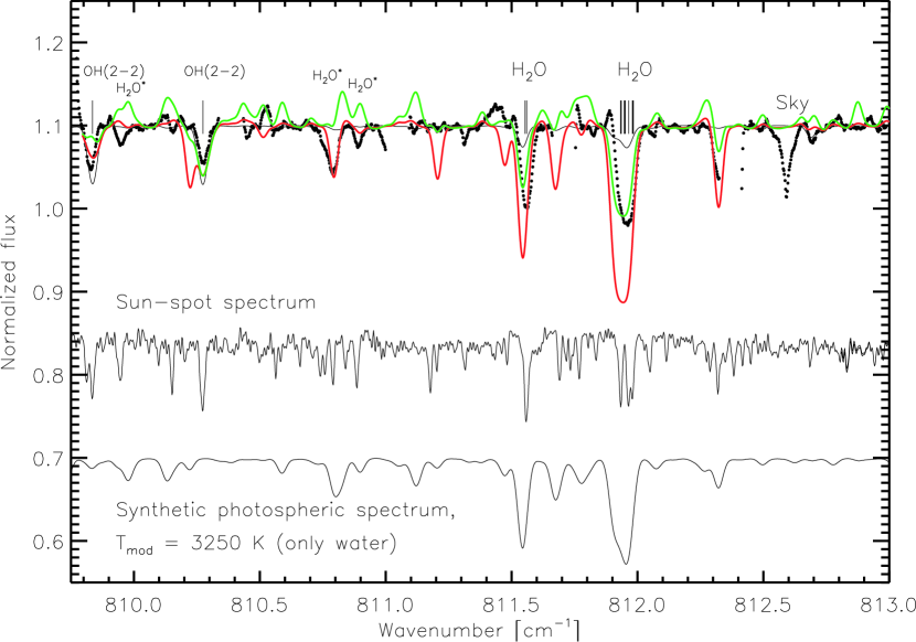
Figure 7: Two normalized spectra of the $809.8-813.0\,$cm^-1 region calculated for two MOLsphere realizations are shown by the green and red lines. The MOLsphere is assumed to contain only water vapor at a temperature of $T=1500$ K and has a column density of water vapor of $N_{\mathrm{col}}=10^{20}$ cm^-2, as described in Tsuji (2000b). Absorption lines are formed but weakened by emission from an extended MOLsphere. We have modeled the layer extending from the surface of the star to a radius of 1.45 (red) and 1.6 stellar radii (green). The more extended the model, the more emission will ‘fill in’ the absorption lines. The underlying photospheric spectrum is shown by the full line normalized to one. Our observed TEXES spectrum is shown by dots. For clarity we have shifted these normalized spectra up by 0.1. To be able to make a comparison, we also show the sun-spot spectrum shifted down to 0.85 and the normalized water-vapor spectrum of our cooler model photosphere shifted down to 0.7. These are the same spectra also shown in Figure 4. In all the synthesized spectra the water-vapor line list by Partridge & Schwenke (1997) is used and the dust emission contribution of 28% is taken into account. All relevant lines (such as OH) are included in the underlying photospheric spectrum. It should be noted that the underlying photospheric spectrum is not identical to the one shown in Figure 1, the reason being the different line lists used. The water-vapor line list used here is more complete but its wavelengths are not accurate enough for our high-resolution spectra. This explains that the lines do not match the observed lines perfectly. The ordinate scale is the same as in Figures 1-6.

Tsuji (2000b) interprets absorption features in the near-infrared as non-photospheric water vapor. The MOLsphere needed to model these data has a column density of water vapor of $N_{\mathrm{col}}=10^{20}$ cm^-2 and a temperature of $T=1500\pm 500$ K. The size of the MOLsphere is not constrained. Due to the large column density of water-vapor and the low temperature needed to fit the near-infrared bands of water vapor, deep absorption lines are supposed to be formed but weakened by emission from an extended MOLsphere (Tsuji, 2000b). We have modeled such a MOLsphere with our photospheric model as the underlying light source. In Figure 7 we plot such a MOLsphere with two different extensions, namely a layer extending from the surface of the star to a radius of 1.45 and one extending to 1.6 stellar radii. The more extended the model, the more emission will ‘fill in’ the absorption lines. The model extending out to 1.45 $R_{\star}$ overestimates the strong lines, but fits a few weak ones. As we extend the MOLsphere out to 1.6 stellar radii, the two strongest water-vapor lines are well matched. However, a majority of the lines are in emission, which is not seen in the observed spectra. The relative strengths of the water lines are not reproduced. The line at approximately 810.8 cm^-1 is best fitted by the model extending out to 1.45 $R_{\star}$, but we also note that a few lines, which are not seen in the observed spectra, appear in the synthetic spectra based on the extension out to 1.45 $R_{\star}$. These are, for example, lines lying at 810.2, 811.2, 814.55, and 819.45 cm^-1. This indicates that the temperature of the MOLsphere is not correct. The extension of the sphere can be tuned to fit a few lines but not others. Thus, this MOLsphere model, with $T=1500$ K, does not fit our spectra well.

A similar but warmer MOLsphere was modeled by Ohnaka (2004b). This water-vapor layer surrounding Betelgeuse was invoked in order to explain partly mid-infrared, high-resolution spectra and partly the increasing diameter of Betelgeuse found by interferometric measurements, from the K band to the $11\,\mu\mathrm{m}$ region. It was argued that the larger angular size in the mid-infrared originated from a MOLsphere containing water vapor. The layer suggested by Ohnaka (2004b), with water lines of optical thickness ranging from $\tau=0.1$ to $10$, also contributes both absorption and emission, due to its geometrical extension. As was shown by Ohnaka (2004b), his layer will not show strong water-vapor absorption in the mid-infrared region, contrary to what we observe. The column density of this realization of a MOLsphere surrounding Betelgeuse is $N_{\mathrm{col}}=2\times 10^{20}$ cm^-2 and the best fit to the data requires a temperature of $T=2050$ K (Ohnaka, 2004b). It extends from the star out to a radius of 1.45 stellar radii. In figure 8 the MOLsphere spectrum is shown together with a part of our observations. The synthetic spectrum shows a large overall emission compared to the photospheric continuum level. The synthetic spectrum consists mostly of a large number of emission lines that blend into each other. Therefore, setting the normalization level, for the comparison with the normalized observed spectrum, is difficult. We have chosen to show the spectrum as calculated, normalized to the photospheric continuum. Clearly the spectrum does not fit our high-resolution spectra, even if we allow for a different normalization. Thus, based on our new data we can directly rule out such a warm MOLsphere with a large column density surrounding Betelgeuse. We note here that in order to explain their multi-wavelength, interferometric observations of $\alpha$ Ori, Perrin et al. (2004a) use an optically thick ($\tau_{11.15\mu\rm{m}}=2.3\pm 0.2$) molecular layer with a temperature of approximately $2050\,\rm{K}$ at $0.3\,\rm{R}_{\star}$ above the photosphere, similar to the one argued for by Ohnaka (2004b). We can, however, rule out such a scenario based on our high-resolution spectra.

Recently, Verhoelst et al. (accepted by A&A) modeled the extended atmospheric environment of Betelgeuse in detail. To model both the near-infrared ISO spectrum ($2.4-45\,\mu\mathrm{m}$) and infrared interferometric information, they suggest the existence of an optically-thin layer of water vapor situated in a shell surrounding the star from approximately 1.3 to 1.45 stellar radii with a column density of $N_{\mathrm{col}}=2\times 10^{19}$ cm^-2 and a temperature of 1750 K. This layer can explain the overall appearance of the medium-resolution ($R\sim 1500$) ISO spectrum. Furthermore, they suggest that the size increase from the K band to the mid-infrared can be explained by opacity from dust grains of alumina (Al₂O₃) instead of the water-vapor layer suggested by Ohnaka (2004b). Verhoelst et al. show that the column densities suggested by Ohnaka (2004b) are too large to be compatible with the near-infrared data. In Figure 9 we show the synthetic spectrum of the realization of the MOLsphere presented in Verhoelst et al. Due to the extension of the MOLsphere and its temperature, the spectrum will, however, be dominated by emission lines. Therefore, not even this MOLsphere realization fits our new data.

Jennings & Sada (1998) modeled their low-resolution, $12\,\mu\mathrm{m}$ spectra with a plane-parallel, isothermal layer close to the location of the onset of the chromospheric temperature rise with $N_{\mathrm{col}}=3\times 10^{18}$ cm^-2 and a temperature of $T_{L}<2800$ K. We have, therefore, simulated this scenario with a very thin MOLsphere on top of the photosphere. We have assumed the MOLsphere to extend from the stellar surface out to 1.01 stellar radii. We find the best fit for a temperature 100 K warmer than the upper limit found by Jennings & Sada (1998), see Figure 10. We see that the strongest water lines are fitted well, but we also see that there might be several water-vapor lines which are modeled too strong. We will discuss this model further in the next section.

As a summary, the realizations of a MOLsphere which have been presented in the literature in order to explain signatures that can not be explained by classical model photospheres do not fit our high-resolution, mid-infrared spectra. Further investigations of the $12\,\mu\mathrm{m}$ lines formed in a MOLsphere with an underlying photosphere would be interesting.

6.2 Can a cooler photosphere explain our spectra?

Another way of looking at the water layer that Jennings & Sada (1998) introduce in order to explain their spectra, is that it represents a cooler outer photospheric structure where water is formed. Thus, also inspired by the explanation of the unexpected water-vapor lines in the $12\,\mu\mathrm{m}$ spectrum of Arcturus and the fact that the line widths and radial velocities of the water-vapor lines in $\alpha$ Ori match that of the photosphere (similar to the case of Arcturus), we have investigated whether a cooling of the temperature structure in the outer photosphere could even fit the observed $12\,\mu\mathrm{m}$ lines. The water-vapor features, which are formed relatively far out in the photosphere, are very sensitive to the temperature where they are formed, much more so than the OH lines. Given the complicating factors of the Betelgeuse photosphere compared to a one-dimensional, hydrostatic model photosphere, accounted for in Section 3, it might not be surprising that a classical model fails to reproduce spectra at all wavelengths. Indeed, because OH and H₂O lines respond differently to temperature variations, a synthetic spectrum calculated from a photosphere of 3250 K (i.e. 350 K cooler), resembles the observed spectrum much better (see Figures 4-6). The fit of the water lines from the ground and first excited vibrational states is much better. The model also predicts the OH lines better, especially OH($v=2-2$). Note that this model is only used to simulate cool photospheric surface regions (e.g. inhomogeneities) or a cooler outer photospheric structure at the line-forming regions of the observed lines.

It is interesting to note that the column density of water all the way through our cooler model photosphere is $5\times 10^{18}$ cm^-2 which is close to what Jennings & Sada (1998) found, namely $(3\pm 2)\times 10^{18}$ cm^-2. Also, our excitation temperature, which we estimated from Equation 3, of $2600\pm 200$ K is close to the temperature estimated by Jennings & Sada (1998). This temperature is also reached deeper in our cooler model, at $\log\tau_{\mathrm{Ross}}\sim-2.2$. These facts explain the good fit to our spectra.

Thus, it seems that our cool model, which can be seen as representing a colder temperature structure in the line-forming regions, can explain the line widths (of the same order as the photospheric macroturbulence), relative line strengths, and column density required. Our spectra are fitted well by our new model.

The effective temperature of our model photosphere that we need in order to model the spectra is too low to be compatible with other spectroscopically (optically and near-infrared) determined effective temperatures of Betelgeuse. The optical and near-infrared spectrum of Betelgeuse can not be modeled by a model photosphere of such a cold temperature, see for example Verhoelst et al. (A&A in press). However, it is not unexpected that the outer photospheric structure could be colder, affecting only the mid-infrared region, in analogy with the case of Arcturus (Ryde et al., 2002), or because the photosphere of Betelgeuse is inhomogeneous. Cool areas may dominate the spectral features in the mid-infrared with the hot areas, in principle, only contributing extra continuous flux, depending on the temperatures and filling factors involved. Measurements in the optical wavelength region are more biased towards hot spots or hotter areas, while cold areas do not contribute much flux. For example, a 3100 K model has only $25\%$ lower flux in the mid-infrared, whereas in the optical the flux drops by a factor of 30 as compared with a 3600 K model. Our exercise shows, that for the line-forming regions, a 3250 K model photosphere could be a better representation of that part of the photosphere. The effect of this cooler outer structure on the near-infrared spectrum will have to be investigated. The site of formation of the absorption lines at $12\,\mu\mathrm{m}$ could be a combination of both the photosphere and a MOLsphere.

Thus, it would be worthwhile to analyse the influence of the physical structure of the outer photosphere on the spectra, for example, by relaxing the assumption of LTE in the calculation of the photospheric structure (see, for example, the case of Arcturus in Short & Hauschildt, 2003). Furthermore, it would be worth investigating the effects on the lines introduced by photospheric inhomogeneities. The observed water-vapor lines may also put constraints on 3-dimensional modeling of supergiants. The challenge for any model including a more realistic atmosphere including, a sophisticated photosphere and a MOLsphere, is that it should not contradict any known, observed spectral features. We will investigate this possibility in a forthcoming paper.

7 Conclusions

We have observed high-resolution, mid-infrared spectra of Betelguese which we have demonstrated to be difficult to explain in existing atmospheric scenarios. For example, a classical model photosphere is not able to explain our spectra, nor is published MOLsphere models which explain other observational discrepancies. We are, however, able to fit our observations with a synthetic spectrum based on a cooler (outer) photospheric temperature structure, as compared with a temperature structure calculated from a classical photospheric modelling.

Thus, the supposed non-classical and/or inhomogeneous outer structures of the photospheres may play a role and may have to be taken into account as a complement to the emergent scenario of a MOLsphere, at least for supergiants. It is clear that, when discussing the outer atmosphere, we require an understanding of the underlying photosphere in its whole complexity, since it will be the underlying illumination of any circumstellar matter. The classical modeling of the outer photosphere of Betelgeuse is most probably also uncertain given the neglect of the mechanical energy and momentum deposition that leads to the chromospheric emission and mass loss.

Further investigations have to be made to reconcile the different emerging pictures of the puzzling atmosphere of Betelgeuse with the aim to be able to explain its entire spectrum in one united scenario. Clearly, it is essential that all aspects and complexities of the photosphere must be investigated, including inhomogeneities, non-standard photospheric structures, etc.

One of the characteristics of the putative MOLspheres is the presence of envelopes which either have large density scale-heights, or discrete shells, overlying the photosphere, which in turn has relatively small density scale-heights. Interferometry with the Atacama Large Millimeter Array (ALMA) may be able to test for the presence of the large density scale-heights or narrow shells associated with these MOLspheres. Centimeter radio continuum interferometry with the Vary Large Array has already been used to map the density scale-heights in the inner wind and chromosphere (Harper et al., 2001), and at 7 mm (43 GHz) the angular diameter of Betelgeuse is 90 mas (Lim et al., 1998). This is larger than the size of the MOLspheres, however, and similar measurements with ALMA at higher frequencies, i.e., 100-700 GHz, will resolve the angular diameter of the atmosphere and probe deeper in towards the photosphere. Measurements of the angular diameter as a function of frequency will provide a direct test of the density structure and of the existence of MOLspheres.

Figure 1: High-resolution spectra of Betelgeuse in the $12\,\micron$ region, here $809.75-813.0\,$cm^-1(dots), are shown. The observations are corrected for the star’s velocity at the time of observation. The wavelengths are thus the laboratory wavelengths. Uppermost in the Figure, the sky spectrum is shown. The almost vertical lines show the ranges of the spectral orders. In this figure five orders are present. Overlaid on the observed Betelgeuse spectrum is a spectrum calculated on the basis of a classical, one-dimensional model atmosphere ($\rm{T}_{\mathrm{eff}}=3600$ K) with, most importantly, OH and water-vapor lines, but also weak metal lines (full line). Only a subset of water-vapor lines in the wavelength region is included. The water-vapor lines included are those with accurately measured wavelengths. A few other water-vapor lines are marked with an asterisk. Shifted vertically downwards from the observed Betelgeuse spectra is shown first the sunspot spectrum of this area. Next below is shown a pure water-vapor spectrum, based on the NASA-Ames water-vapor line list for a Betelgeuse model. Note that the NASA-Ames list includes a large number of lines but that the wavelengths are not accurate enough for this resolution. Each OH and H₂O line included is indicated by a vertical line, independent of their strengths.

Figure 2: For caption see Figure 1. The model spectrum shown is based on a model photosphere of an effective temperature of $\rm{T}_{\mathrm{eff}}=3600$ K. Here the wavelength region $814.3-816.8\,$cm^-1 is shown.

Figure 3: For caption see Figure 1. The model spectrum shown is based on a model photosphere of an effective temperature of $\rm{T}_{\mathrm{eff}}=3600$ K. Here the wavelength region $817.0-820.4\,$cm^-1 is shown.

Figure 4: These spectra show our $\alpha$ Ori observations in the same way as in Figure 1. However, the model comparison is that based on a slightly cooler model photosphere ($T_{\mathrm{mod}}=3250\,$ K).

Figure 5: For caption see Figure 4. The model spectrum shown is based on a model photosphere of an effective temperature of $\rm{T}_{\mathrm{mod}}=3250$ K. Here the wavelength region $814.3-816.8\,$cm^-1 is shown.

Figure 6: For caption see Figure 4. The model spectrum shown is based on a model photosphere of an effective temperature of $\rm{T}_{\mathrm{mod}}=3250$ K. Here the wavelength region $817.0-820.4\,$cm^-1 is shown.

Figure 8: The same figure as in Figure 7, except that the realization of the MOLsphere is based on the one suggested by Ohnaka (2004b). The calculated MOLsphere spectrum with our underlying photospheric spectrum based on a Betelgeuse model of 3600 K, is shown as the upper-most spectrum. This spectrum is normalized to the photospheric spectrum, and is therefore mostly in emission, due to the combination of its geometrical extension the column density of $N_{\mathrm{col}}=2\times 10^{20}$ cm^-2 and temperature of of $T=2050$ K (Ohnaka, 2004b). This MOLsphere extends from the star out to a radius of 1.45 stellar radii. Also in this figure, we show the sun-spot spectrum shifted down to 0.85 and the normalized water-vapor spectrum of our cooler model photosphere shifted down to 0.7.

Figure 9: In principle the same figure as in Figure 7, except that the realization of the MOLsphere is that suggested by Verhoelst et al. (accepted by A&A). The wavelength region is different compared to Figure 7. The emergent spectrum of the $817.0-820.4\,$cm^-1 region is displayed by the thick line, mostly showing emission lines. The optically-thin layer of water vapor is situated in a shell surrounding the star from approximately 1.3 to 1.45 stellar radii with a column density of $N_{\mathrm{col}}=2\times 10^{19}$ cm^-2 and a temperature of 1750 K. The dots shows our TEXES observations and the spectrum shifted down to 0.7 is a normalized, pure water-vapor spectrum based on our cold Betelgeuse model of 3250 K and the line list by Partridge & Schwenke (1997). The sun-spot spectrum shifted down to 0.85 is also shown. The underlying photospheric spectrum is shown by the full line normalized to one.

Figure 10: Similar figure as in Figures 7-9. This MOLsphere realization simulates the case presented in Jennings & Sada (1998): $N_{\mathrm{col}}=3\times 10^{18}$ cm^-2 and a temperature of $T_{L}<2800$ K. The MOLsphere extends from the stellar surface out to 1.01 stellar radii. We find the best fit for a temperature of 2900 K. The MOLsphere spectrum is shown by a thick full line. The strong lines are modeled well but several other lines are modeled too strong. The underlying photospheric spectrum is shown by the full line normalized to one. The observations are shown by dots. The normalized spectrum shifted down to 0.7 is a pure water-vapor spectrum based on our cold Betelgeuse model of 3250 K and the line list by Partridge & Schwenke (1997). For comparison the sun spot spectrum is also shown.

References

- (1)
- Bernat et al. (1979) Bernat, A. P., Hall, D. N. B., Hinkle, K. H., & Ridgway, S. T., 1979, ApJ, L135
- Bernath (2002) Bernath, P. F. 2002, Physical Chemistry-Chemical Physics, 4, 1501
- Bester et al. (1996) Bester, M., Danchi, W. C., Hale, D., et al. 1996, ApJ, 463, 336
- Carpenter & Robinson (1997) Carpenter, K. G. & Robinson, R. D. 1997, ApJ, 479, 970
- Carr et al. (2000) Carr, J. S., Sellgren, K., & Balachandran, S. C. 2000, ApJ, 530, 307
- Cox (2000) Cox, A. N. 2000, Allen’s astrophysical quantities (Allen’s astrophysical quantities, 4th ed. Publisher: New York: AIP Press; Springer, 2000. Editedy by Arthur N. Cox. ISBN: 0387987460)
- Dupree et al. (1990) Dupree, A. K., Baliunas, S. L., Hartmann, L., Guinan, E. F., & Sonneborn, G. 1990, in Astronomical Society of the Pacific Conference Series, Vol. 11, 468
- Dupree et al. (1987) Dupree, A. K., Baliunas, S. L., Hartmann, L., et al. 1987, ApJ, 317, L85
- Dupree & Gilliland (1995) Dupree, A. K. & Gilliland, R. L. 1995, Bulletin of the American Astronomical Society, 27, 1328
- Edvardsson et al. (1993) Edvardsson, B., Andersen, J., Gustafsson, B., et al. 1993, A&A, 275, 101
- Freytag (2003) Freytag, B. 2003, Astronomische Nachrichten Supplement, 324, 67
- Freytag & Mizuno-Wiedner (2003) Freytag, B. & Mizuno-Wiedner, M. 2003, in IAU Symposium 210: ’Modelling of Stellar Atmospheres , Eds. N. Piskunov, W. W. Weiss, and D. F. Gray, CD–C4
- Freytag et al. (2002) Freytag, B., Steffen, M., & Dorch, B. 2002, Astronomische Nachrichten, 323, 213
- Gilliland & Dupree (1996) Gilliland, R. L. & Dupree, A. K. 1996, ApJ Lett., 463, L29
- Glassgold & Huggins (1986) Glassgold, A. E. & Huggins, P. J. 1986, ApJ, 306, 605
- Goldberg (1979) Goldberg, L. 1979, QJRAS, 20, 361
- Goldberg (1984) Goldberg, L. 1984, PASP, 96, 366
- Goldman et al. (1998) Goldman, A., Schoenfeld, W., Goorvitch, D., et al. 1998, JQSRT, 59, 453
- Gray (1992) Gray, D. F. 1992, The observation and analysis of stellar photospheres (Cambridge Astrophysics Series, Cambridge: Cambridge University Press, 1992, 2nd ed., ISBN 0521403200.)
- Gray (2000) Gray, D. F. 2000, ApJ, 532, 487
- Gray (2001) Gray, D. F. 2001, PASP, 113, 1378
- Gustafsson et al. (1975) Gustafsson, B., Bell, R. A., Eriksson, K., & Nordlund, A. 1975, A&A, 42, 407
- Gustafsson et al. (2003) Gustafsson, B., Edvardsson, B., Eriksson, K., et al. 2003, in IAU Symposium 210: ’Modelling of Stellar Atmospheres , Eds. N. Piskunov, W. W. Weiss, and D. F. Gray, CD–A4
- Harper et al. (2001) Harper, G. M., Brown, A., & Lim, J. 2001, ApJ, 551, 1073
- Hinkle & Barnes (1979) Hinkle, K. H. & Barnes, T. G. 1979, ApJ, 227, 923
- Hinkle & Lambert (1975) Hinkle, K. H. & Lambert, D. L. 1975, MNRAS, 170, 447
- Huggins (1987) Huggins, P. J. 1987, ApJ, 313, 400
- Jennings et al. (1986) Jennings, D. E., Deming, D., Wiedemann, G. R., & Keady, J. J. 1986, ApJ Lett., 310, L39
- Jennings & Sada (1998) Jennings, D. E. & Sada, P. V. 1998, Science, 279, 844
- Jørgensen et al. (1992) Jørgensen, U. G., Johnson, H. R., & Nordlund, Å. 1992, A&A, 261, 263
- Keenan & McNeil (1989) Keenan, P. C. & McNeil, R. C. 1989, ApJS, 71, 245
- Lacy et al. (2002) Lacy, J. H., Richter, M. J., Greathouse, T. K., Jaffe, D. T., & Zhu, Q. 2002, PASP, 114, 153
- Lambert et al. (1984) Lambert, D. L., Brown, J. A., Hinkle, K. H., & Johnson, H. R. 1984, ApJ, 284, 223
- Lim et al. (1998) Lim, J., Carilli, C. L., White, S. M., Beasley, A. J., & Marson, R. G. 1998, Nature, 392, 575
- Lobel & Dupree (2000) Lobel, A. & Dupree, A. K. 2000, ApJ, 545, 454
- Ludwig et al. (2003) Ludwig, H., Freytag, B., Höfner, S., Allard, F., & Hauschildt, P. H. 2003, in IAU Symposium 219: ’Stars as Suns: Activity, Evolution, and Planets’, E41
- Matsuura et al. (1999) Matsuura, M., Yamamura, I., Murakami, H., Freund, M. M., & Tanaka, M. 1999, A&A, 348, 579
- Mennesson et al. (2002) Mennesson, B., Perrin, G., Chagnon, G., et al. 2002, ApJ, 579, 446
- Morgan et al. (1997) Morgan, N. D., Wasatonic, R., & Guinan, E. F., 1997, IBVS, No. 4499
- Ohnaka (2004a) Ohnaka, K. 2004a, A&A, 424, 1011
- Ohnaka (2004b) Ohnaka, K. 2004b, A&A, 421, 1149
- Partridge & Schwenke (1997) Partridge, H. & Schwenke, D. 1997, J. Chem. Phys., 106, 4618
- Perrin et al. (2004a) Perrin, G., Ridgway, S. T., Coudé du Foresto, V., et al. 2004a, A&A, 418, 675
- Perrin et al. (2004b) Perrin, G., Ridgway, S. T., Mennesson, B., et al. 2004b, A&A, 426, 279
- Piskunov et al. (1995) Piskunov, N. E., Kupka, F., Ryabchikova, T. A., Weiss, W. W., & Jeffery, C. S. 1995, A&AS, 112, 525
- Plez et al. (1992) Plez, B., Brett, J. M., & Nordlund, Å. 1992, A&A, 256, 551
- Polyansky et al. (1996) Polyansky, O. L., Busler, J. R., Guo, B., Zhang, K., & Bernath, P. F. 1996, J. Mol. Spectrosc., 176, 305
- Polyansky et al. (1997a) Polyansky, O. L., Tennyson, J., & Bernath, P. F. 1997a, J. Mol. Spectrosc., 186, 213
- Polyansky et al. (1997b) Polyansky, O. L., Zobov, N. F., Viti, S., et al. 1997b, J. Mol. Spectrosc., 186, 422
- Ryde et al. (2005) Ryde, N., Gustafsson, B., Eriksson, K., & Wahlin, R. 2005, in ‘High Resolution Infrared Spectroscopy in Astronomy’, Proceedings of the ESO Workshop held in Garching Nov. 18-21. 2004, ed. H. Kaeufl, R. Siebenmorgen, & A. Moorwood, Vol. in press (Berlin: Springer Verlag)
- Ryde et al. (2003a) Ryde, N., Lacy, J. H., Richter, M. J., Lambert, D. L., & Greathouse, T. K. 2003a, in ’Modelling of Stellar Atmospheres’, Proceedings of the IAU Symposium 210, ed. N. Piskunov, W. W. Weiss, & D. F. Gray, CD–E67
- Ryde et al. (2003b) Ryde, N., Lacy, J. H., Richter, M. J., Lambert, D. L., & Greathouse, T. K. 2003b, in ASSL Vol. 283: Mass-Losing Pulsating Stars and their Circumstellar Matter, 227
- Ryde et al. (2002) Ryde, N., Lambert, D. L., Richter, M. J., & Lacy, J. H. 2002, ApJ, 580, 447
- Ryde et al. (2003c) Ryde, N., Lambert, D. L., Richter, M. J., Lacy, J. H., & Greathouse, T. K. 2003c, in ASP Conf. Ser. 293: 3D Stellar Evolution, 214
- Sanford (1933) Sanford, R. F. 1933, ApJ, 77, 110
- Schuller et al. (2004) Schuller, P., Salomé, P., Perrin, G., et al. 2004, A&A, 418, 151
- Schwarzschild (1975) Schwarzschild, M. 1975, ApJ, 195, 137
- Short & Hauschildt (2003) Short, C. I. & Hauschildt, P. H. 2003, ApJ, 596, 501
- Skinner & Whitmore (1987) Skinner, C. J. & Whitmore, B. 1987, MNRAS, 224, 335
- Sloan et al. (2003) Sloan, G. C., Kraemer, K. E., Price, S. D., & Shipman, R. F. 2003, ApJS, 147, 379
- Smith et al. (1989) Smith, M. A., Patten, B. M., & Goldberg, L. 1989, AJ, 98, 2233
- Spencer Jones (1928) Spencer Jones, H. 1928, MNRAS, 88, 660
- Sudol et al. (1999) Sudol, J. J., Dyck, H. M., Stencel, R. E., Klebe, D. I., & Creech-Eakman, M. J. 1999, AJ, 117, 1609
- Tej et al. (2003a) Tej, A., Lançon, A., & Scholz, M. 2003a, A&A, 401, 347
- Tej et al. (2003b) Tej, A., Lançon, A., Scholz, M., & Wood, P. R. 2003b, A&A, 412, 481
- Tsuji (2000a) Tsuji, T. 2000a, ApJ Lett., 540, L99
- Tsuji (2000b) Tsuji, T. 2000b, ApJ, 538, 801
- Tsuji (2001a) Tsuji, T. 2001a, in IAU Symposium 205: ’Galaxies and their Constituents at the Highest Angular Resolutions , Ed. R. T. Schilizzi, 316
- Tsuji (2001b) Tsuji, T. 2001b, A&A, 376, L1
- Tsuji (2003) Tsuji, T., 2003, in ESA SP-511: Exploiting the ISO Data Archive. Infrared Astronomy in the Internet Age, p. 93
- Tsuji et al. (1997) Tsuji, T., Ohnaka, K., Aoki, W., & Yamamura, I. 1997, A&A, 320, L1
- Tsuji et al. (1998) Tsuji, T., Ohnaka, K., Aoki, W., & Yamamura, I. 1998, Ap&SS, 255, 293
- Tuthill et al. (1997) Tuthill, P. G., Haniff, C. A., & Baldwin, J. E. 1997, MNRAS, 285, 529
- Verhoelst et al. (2003) Verhoelst, T., Decin, L., Vandenbussche, B., Van Malderen, R., & Waelkens, C. 2003, in IAU Symposium 210: ’Modelling of Stellar Atmospheres , Eds. N. Piskunov, W. W. Weiss, and D. F. Gray, CD–E14
- Wallace et al. (1995) Wallace, L., Bernath, P., Livingston, W., et al. 1995, Science, 268, 1155
- Wallace et al. (1994) Wallace, L., Livingston, W., & Bernath, P. 1994, An atlas of the sunspot spectrum from to ( to micrometer) and the photospheric spectrum from to ( to micrometer) (NSO Technical Report, Tucson: National Solar Observatory, National Optical Astronomy Observatory)
- Weiner (2004) Weiner, J. 2004, ApJ, 611, L37
- Weiner et al. (2003) Weiner, J., Hale, D. D. S., & Townes, C. H. 2003, ApJ, 589, 976
- Wilson et al. (1997) Wilson, R. W., Dhillon, V. S., & Haniff, C. A. 1997, MNRAS, 291, 819
- Woitke et al. (1999) Woitke, P., Helling, C., Winters, J. M., & Jeong, K. S. 1999, A&A, 348, L17
- Woolf et al. (1964) Woolf, N. J., Schwarzschild, M., & Rose, W. K. 1964, ApJ, 140, 833
- Yamamura et al. (1999) Yamamura, I., de Jong, T., & Cami, J. 1999, A&A, 348, L55
- Young et al. (2000) Young, J. S., Baldwin, J. E., Boysen, R. C., et al. 2000, MNRAS, 315, 635