3D Gasdynamic Modelling of the Changes in the Flow Structure During Transition From Quiescent to Active State in Symbiotic Stars

Abstract

The results of 3D modelling of the flow structure in the classical symbiotic system Z Andromedae are presented. Outbursts in systems of this type occur when the accretion rate exceeds the upper limit of the steady burning range. Therefore, in order to realize the transition from a quiescent to an active state it is necessary to find a mechanism able to sufficiently increase the accretion rate on a time scale typical to the duration of outburst development.

Our calculations have confirmed the transition mechanism from quiescence to outburst in classic symbiotic systems suggested earlier on the basis of 2D calculations (Bisikalo et al, 2002). The analysis of our results have shown that for wind velocity of 20 km/s an accretion disc forms in the system. The accretion rate for the solution with the disc is $\sim 22.5-25\%$ of the mass loss rate of the donor, that is,  $\sim 4.5-5\cdot 10^{-8}$ $M_{\odot}$/yr for Z And. This value is in agreement with the steady burning range for white dwarf masses typically accepted for this system. When the wind velocity increases from 20 to 30 km/s the accretion disc is destroyed and the matter of the disc falls onto the accretor’s surface. This process is followed by an approximately twofold accretion rate jump. The resulting accretion rate growth is sufficient for passing the upper limit of the steady burning range, thereby bringing the system into an active state. The time during which the accretion rate is above the steady burning value is in a very good agreement with observations.

The analysis of the results presented here allows us to conclude that small variations in the donor’s wind velocity can lead to the transition from the disc accretion to the wind accretion and, as a consequence, to the transition from quiescent to active state in classic symbiotic stars.

1 Introduction

Symbiotic stars are characterized by peculiar spectra where molecular absorption bands - the characteristic features of a cool giant - are present together with emission lines corresponding to a high excitation level. The red and infrared spectra of symbiotic stars are typical of cool giants while in the UV range they are characterized by a very hot continuum. It is widely assumed that most symbiotic stars are detached binaries consisting of a cool giant and a white dwarf surrounded by a nebulosity [1]. Mass exchange in these systems is driven by stellar wind.

The goal of this work is to carry out a study of classical symbiotic systems using as example one of the most well-studied representatives of this class - Z And. According to the analyses of its energy distribution in a wide spectral range [2], the components of Z And have the following characteristics: the cool M3.5III giant has a mass $\sim 2~{}M_{\odot}$ and a radius $\sim$ 100$R_{\odot}$, while the white dwarf has a mass $\sim 0.6~{}M_{\odot}$, a radius $\sim$ 0.07$R_{\odot}$ and a temperature $\sim 10^{5}$ K. The giant loses mass at the rate of $\sim 2\times 10^{-7}~{}M_{\odot}$/yr. Gas in the circumbinary envelope has an electron density of $\sim 2\cdot 10^{10}~{}\mbox{cm}^{-3}$ and a temperature $\sim 1.5\div 8\cdot 10^{4}$ K. The separation of the system is 482$R_{\odot}$, the orbital period is 758 days. More than 100 years of observations have shown that this star presents outbursts. The last of them took place in 2000 and has been actively observed at different wavelengths.

Following the characteristics of their outbursts, symbiotic stars can be divided in two types [3, 4]. The first type includes so-called classical symbiotics (e.g. Z And, AG Peg, AG Dra, CI Cyg, AX Per). Their outbursts typically last a few months and have amplitudes of 2-4^m. The typical feature of such outbursts is the weakening of high excitation lines while the brightness increases. The detailed description of the behaviour of these stars is given in [5, 6]. Symbiotic novae (e.g. V1016 Cyg, V1329 Cyg, RS Oph, HM Sge) show the second type of outbursts. These outbursts are longer and brighter. Their energetics can even exceed that of novae outbursts. The principal difference of these outbursts from those of the first type is the increase of the ionization degree while the brightness increases. The behaviour of these stars during outbursts is described in [7, 8, 9,10]. The second type of outbursts is similar to slow classical novae outbursts [11, 12] (for differences between symbiotic novae and slow classical novae outbursts see [13]).

The most probable mechanism describing the observational manifestations of classical symbiotics as well as of symbiotic novae is thermonuclear burning on the accretor’s surface [see, e.g. 6, 13]. It has been shown in various works [14, 15, 3, 16, 17] that the process of thermonuclear burning of hydrogen on the white dwarf surface strongly depends on the accretion rate ${\raisebox{1.0pt}{\hbox{$\stackrel{{\scriptstyle\bullet}}{{M}}$}}}\ \!\!^{accr}$ [3]. Only, in a narrow range of ${\raisebox{1.0pt}{\hbox{$\stackrel{{\scriptstyle\bullet}}{{M}}$}}}\ \!\!^{accr}$ is the steady hydrogen burning possible [15, 18, 19]. The lower limit of this range is given by the expression [20,16]

$${\raisebox{1.0pt}{\hbox{$\stackrel{{\scriptstyle\bullet}}{{M}}$}}}\ \!\!_{steady,min}=1.3\cdot 10^{-7}\cdot\left(\frac{M}{M_{\odot}}\right)^{3.57}M_{\odot}/\mbox{yr}\,,$$

while the higher limit is given by [22, 23]

$${\raisebox{1.0pt}{\hbox{$\stackrel{{\scriptstyle\bullet}}{{M}}$}}}\ \!\!_{steady,max}=6\cdot 10^{-7}\cdot\left(\frac{M}{M_{\odot}}-0.522\right)M_{\odot}/\mbox{yr}\,,$$

For Z And where $M=0.6M_{\odot}$, steady burning is possible in the range $2.1\cdot 10^{-8}M_{\odot}/\mbox{yr}\ {\raise-2.15277pt\hbox{$\buildrel<\over{\scriptstyle\sim}$}}\ {\raisebox{1.0pt}{\hbox{$\stackrel{{\scriptstyle\bullet}}{{M}}$}}}\ \!\!^{accr}\ {\raise-2.15277pt\hbox{$\buildrel<\over{\scriptstyle\sim}$}}\ 4.7\cdot 10^{-8}M_{\odot}/\mbox{yr}$. If the accretion rate is below this interval, thermonuclear burning exhausts the matter faster than accretion can replenish it bringing the burning to a halt. Following this, hydrogen begins to accumulate on the white dwarf surface until the pressure near the hydrogen envelope base reaches a critical value and a hydrogen shell flash occurs. The bolometric luminosity increases by a factor 10–100 times in the course of $\sim$ 1 year and stays at the active state for $\sim$ 10 years. The total duration of the outburst is dozens of years that corresponds to the nuclear time scale. This is observed in symbiotic novae.

If for some reason ${\raisebox{1.0pt}{\hbox{$\stackrel{{\scriptstyle\bullet}}{{M}}$}}}\ \!\!^{accr}$ becomes larger than ${\raisebox{1.0pt}{\hbox{$\stackrel{{\scriptstyle\bullet}}{{M}}$}}}\ \!\!_{steady,max}$, the accreted matter accumulates above the burning shell and expands to giant dimensions. Such behaviour is typical for classical symbiotic stars. Though the bolometric luminosity stays constant, the visual brightness increases by 1-2 magnitudes and the effective temperature decreases. Optical outburst develops on the thermal timescale. In accordance with existing models of thermonuclear burning on a white dwarf’ surface [20,15], small variations of the accretion rate can lead to significant changes of the temperature at practically constant bolometric luminosity. For a white dwarf of $1.2M_{\odot}$ mass, an envelope mass change of $4\times 10^{-7}~{}M_{\odot}$ can result in a 3^m luminosity increase [3]. This value corresponds to the typical amplitude of Z And outbursts.

Z And belongs to the class of classical symbiotics and, in accordance with the accepted model, the accretion rate in the quiescent state should be in the steady burning range. For an outburst to develop the accretion rate should become large enough to reach a value above the steady burning range. It should be noted that the time scale of the accretion rate increase should correspond to the characteristic time of outburst development ($\sim 100$ days). Such behaviour of the accretion rate in a binary system is possible in the framework of the mechanism proposed in [21] using results of 2D gasdynamic modelling. The main idea of the mechanism is that even minor variations in the donor’s wind velocity is enough to lead to the accretion regime change - from disc accretion to wind accretion. During the transition period, namely during the disc destruction the accretion rate increases abruptly and exceeds the upper limit of the steady burning range. The goal of this work is to check the possibility of realizing such a mechanism using a more realistic 3D model.

2 The model

In order to study the gas flow structure in the symbiotic system Z And 3D numerical simulations have been carried out. The zero point of the coordinate system was placed at the centre of the accretor, the $x$- axis was directed along the line connecting centres of the components and oppositely to the mass-losing star, the $y$-axis – along the accretor orbital motion, and the $z$-axis – along the axis of rotation of the binary system. The flow was described by the system of Euler equations in corotating coordinate frame:

$${\frac{{\partial\rho}}{{\partial t}}}+{\frac{{\partial\rho u}}{{\partial x}}}+{\frac{{\partial\rho v}}{{\partial y}}}+{\frac{{\partial\rho w}}{{\partial z}}}=0\,,$$

$${\frac{{\partial\rho u}}{{\partial t}}}+{\frac{{\partial(\rho u^{2}+P)}}{{\partial x}}}+{\frac{{\partial\rho uv}}{{\partial y}}}+{\frac{{\partial\rho uw}}{{\partial z}}}=-\rho{\frac{{\partial\Phi}}{{\partial x}}}+2\Omega v\rho\,,$$

$${\frac{{\partial\rho v}}{{\partial t}}}+{\frac{{\partial\rho uv}}{{\partial x}}}+{\frac{{\partial(\rho v^{2}+P)}}{{\partial y}}}+{\frac{{\partial\rho vw}}{{\partial z}}}=-\rho{\frac{{\partial\Phi}}{{\partial y}}}-2\Omega u\rho\,,$$

$${\frac{{\partial\rho w}}{{\partial t}}}+{\frac{{\partial\rho uw}}{{\partial x}}}+{\frac{{\partial\rho vw}}{{\partial y}}}+{\frac{{\partial(\rho w^{2}+P)}}{{\partial z}}}=-\rho{\frac{{\partial\Phi}}{{\partial z}}}\,,$$

$${\frac{{\partial\rho E}}{{\partial t}}}+{\frac{{\partial\rho uh}}{{\partial x}}}+{\frac{{\partial\rho vh}}{{\partial y}}}+{\frac{{\partial\rho wh}}{{\partial z}}}=-\rho u{\frac{{\partial\Phi}}{{\partial x}}}-\rho v{\frac{{\partial\Phi}}{{\partial y}}}-\rho w{\frac{{\partial\Phi}}{{\partial z}}}\,.$$

Here ${{\mathchoice{\hbox{$\displaystyle u$}}{\hbox{$\textstyle u$}}{\hbox{$\scriptstyle u$}}{\hbox{$\scriptscriptstyle u$}}}}=(u,v,w)$ is the velocity vector, $P$ – the pressure, $\rho$ – the density, $h=\varepsilon+P/\rho+|{{\mathchoice{\hbox{$\displaystyle u$}}{\hbox{$\textstyle u$}}{\hbox{$\scriptstyle u$}}{\hbox{$\scriptscriptstyle u$}}}}|^{2}/2$ – the specific total enthalpy, $E=\varepsilon+|{{\mathchoice{\hbox{$\displaystyle u$}}{\hbox{$\textstyle u$}}{\hbox{$\scriptstyle u$}}{\hbox{$\scriptscriptstyle u$}}}}|^{2}/2$ – the specific total energy, $\varepsilon$ – the specific internal energy, $\Omega$ – the angular velocity of binary system’s rotation, and $\Phi({{\mathchoice{\hbox{$\displaystyle r$}}{\hbox{$\textstyle r$}}{\hbox{$\scriptstyle r$}}{\hbox{$\scriptscriptstyle r$}}}})$ – the force potential.

In the standard definition when only the gravitational forces from the point mass components and the centrifugal force are taken into account, the force potential is given by:

$$\Phi({{\mathchoice{\hbox{$\displaystyle r$}}{\hbox{$\textstyle r$}}{\hbox{$\scriptstyle r$}}{\hbox{$\scriptscriptstyle r$}}}})=-\frac{GM_{1}}{|{{\mathchoice{\hbox{$\displaystyle r$}}{\hbox{$\textstyle r$}}{\hbox{$\scriptstyle r$}}{\hbox{$\scriptscriptstyle r$}}}}-{{\mathchoice{\hbox{$\displaystyle r$}}{\hbox{$\textstyle r$}}{\hbox{$\scriptstyle r$}}{\hbox{$\scriptscriptstyle r$}}}}_{1}|}-\frac{GM_{2}}{|{{\mathchoice{\hbox{$\displaystyle r$}}{\hbox{$\textstyle r$}}{\hbox{$\scriptstyle r$}}{\hbox{$\scriptscriptstyle r$}}}}-{{\mathchoice{\hbox{$\displaystyle r$}}{\hbox{$\textstyle r$}}{\hbox{$\scriptstyle r$}}{\hbox{$\scriptscriptstyle r$}}}}_{2}|}-\hbox{$\,{}^{1}\!/_{2}$}\Omega^{2}({{\mathchoice{\hbox{$\displaystyle r$}}{\hbox{$\textstyle r$}}{\hbox{$\scriptstyle r$}}{\hbox{$\scriptscriptstyle r$}}}}-{{\mathchoice{\hbox{$\displaystyle r$}}{\hbox{$\textstyle r$}}{\hbox{$\scriptstyle r$}}{\hbox{$\scriptscriptstyle r$}}}}_{c})^{2}\,.$$

Here $M_{1}$ is the mass of the accretor, $M_{2}$ – the mass-losing star’s mass, ${{\mathchoice{\hbox{$\displaystyle r$}}{\hbox{$\textstyle r$}}{\hbox{$\scriptstyle r$}}{\hbox{$\scriptscriptstyle r$}}}}_{1}$, ${{\mathchoice{\hbox{$\displaystyle r$}}{\hbox{$\textstyle r$}}{\hbox{$\scriptstyle r$}}{\hbox{$\scriptscriptstyle r$}}}}_{2}$ – the radius-vectors of the centres of components, ${{\mathchoice{\hbox{$\displaystyle r$}}{\hbox{$\textstyle r$}}{\hbox{$\scriptstyle r$}}{\hbox{$\scriptscriptstyle r$}}}}_{c}$ – the radius-vector of the centre of mass of the system. This is the so-called Roche potential. But in our case the additional force responsible for the donor’s wind acceleration should also be taken into account. Therefore, the form of the potential changes. Previous studies (e.g., [24–26]) have shown that the general flow structure in the system where components do not fill their Roche lobes is defined first and foremost by the stellar wind parameters. Since the mechanism of gas acceleration is poorly known for cool giants, we mimic the radiation pressure by reducing the gravitational attraction force to the donor star by a factor ($1-\Gamma$). So, the modified force potential looks the following:

$$\Phi({{\mathchoice{\hbox{$\displaystyle r$}}{\hbox{$\textstyle r$}}{\hbox{$\scriptstyle r$}}{\hbox{$\scriptscriptstyle r$}}}})=-(1-\Gamma)\frac{GM_{2}}{|{{\mathchoice{\hbox{$\displaystyle r$}}{\hbox{$\textstyle r$}}{\hbox{$\scriptstyle r$}}{\hbox{$\scriptscriptstyle r$}}}}-{{\mathchoice{\hbox{$\displaystyle r$}}{\hbox{$\textstyle r$}}{\hbox{$\scriptstyle r$}}{\hbox{$\scriptscriptstyle r$}}}}_{2}|}-\frac{GM_{1}}{|{{\mathchoice{\hbox{$\displaystyle r$}}{\hbox{$\textstyle r$}}{\hbox{$\scriptstyle r$}}{\hbox{$\scriptscriptstyle r$}}}}-{{\mathchoice{\hbox{$\displaystyle r$}}{\hbox{$\textstyle r$}}{\hbox{$\scriptstyle r$}}{\hbox{$\scriptscriptstyle r$}}}}_{1}|}-\hbox{$\,{}^{1}\!/_{2}$}\Omega^{2}({{\mathchoice{\hbox{$\displaystyle r$}}{\hbox{$\textstyle r$}}{\hbox{$\scriptstyle r$}}{\hbox{$\scriptscriptstyle r$}}}}-{{\mathchoice{\hbox{$\displaystyle r$}}{\hbox{$\textstyle r$}}{\hbox{$\scriptstyle r$}}{\hbox{$\scriptscriptstyle r$}}}}_{c})^{2}\,.$$

To close the system the perfect gas equation of state was used.

$$P=(\gamma-1)\rho\varepsilon\,,$$

The value of adiabatic index has been accepted $\gamma=1.01$, that corresponds to the case close to the isothermal one [27–29].

We adopted for the parameters of the binary system those of Z And. In our numerical simulations all variables were put in dimensionless form as follows: the length was normalized by the separation of two stars, $A$, and the time by $\Omega^{-1}$, and so the velocity was normalized by $A\Omega$. The density was normalized by that at the surface of the mass-losing star.

The method of computational fluid dynamics is described in [30] and details are explained in [31, 32]. We use the simplified flux vector splitting (SFS) finite volume scheme to discretize the Euler equation (the description of the SFS scheme is given in the appendix of [31]).

We assume a symmetry about the orbital plane, and therefore only compute the upper half-space of the computational domain, which is $-2<x<1$, $-1.5<y<1.5$, $0<z<1.0$. The region is divided into $253\times 253\times 85$ cells. The inner numerical boundary surrounding the mass-losing star is represented by an equipotential surface with a mean radius $R_{2n}$ (we set the numerical boundary at a little larger radius, $R_{2n}=101R_{\odot}$, rather than $R_{2}$). The radius of the mass-accreting star is too small to fit in our numerical grid so it is represented by one cell.

The cells just inside of the inner numerical boundary about the mass-losing star are assumed to be filled with gas with dimensionless density $\rho_{2}=1$, dimensionless sound speed $c_{s}=0.178$ (corresponding to $T_{2}=3200K$), and a dimensionless normal speed to the surface, $V$. The real normal velocity of the gas on the numerical boundary is determined by solving Riemann problems between the cells adjacent to the inner boundary surface. The cell representing the mass-accreting star and the cells just outside of the outer numerical boundary are filled by a gas with density $\rho_{0}=10^{-9}$, pressure $p_{0}=10^{-8}/\gamma$, and three velocity components $u_{0}=v_{0}=w_{0}=0$. This assumption does not mean that accretion onto the mass accreting star nor that escape from the computational domain do not occur. The velocity of the gas on the boundaries are computed by solving Riemann problems. At the initial stage $t=0$, the computational domain except the region inside of the inner boundaries is assumed to be filled by a gas with $\rho_{0}=10^{-9}$, $p_{0}=10^{-8}/\gamma$, and $u_{0}=v_{0}=w_{0}=0.$ This gas is gradually replaced by the gas supplied from the mass-losing star. We compute up to a few rotation periods that is generally long enough for the system to reach a quasi-steady state.

3 Results

The velocity of the mass-losing star’s wind in Z And is $\sim$25 km/s [2]. It is presumed in the framework of the considered mechanism that for slightly smaller velocities an accretion disc will form while for slightly greater values the disc will be destroyed and a wind accretion type of flow will occur. In order to check the applicability of the proposed mechanism, numerical simulations for velocities of 25$\pm 5$km/s have been carried out. Calculations for the wind velocity $V_{w}=20$ km/s were necessary for studying the possibility of disc formation in the system, accretion rate estimation and to check if the accretion rate is indeed within the limits of the steady burning range. Calculations for $V_{w}=30$ km/s were conducted in order to obtain parameters of the flow structure in the system without disc. To answer the questions concerning processes taking place after the wind velocity change – if the disc will be destroyed, how the accretion rate will grow, if the accretion rate change will go above the upper limit of the steady burning range – calculations with a wind velocity jump from $20\rightarrow 30$ km/s have been carried out

The results of our numerical modelling have shown that for wind velocity $V_{w}=20$ km/s and values of the parameter $\Gamma\in[0.85;0.95]$ a steady accretion disc forms in the system. In Figures 1,2 the flow structure for the case $V_{w}=20$ km/s and $\Gamma$=0.94 is shown. Density contours and velocity vectors in the equatorial plane of the system are presented for the whole computational domain (Fig. 1) and for the near-accretor area $[-0.5A\ldots A]\times[-A\ldots 0.5A]$ (Fig. 2). The results of the calculations are presented at the time $t\sim 5P_{orb}$ when a steady regime was already established in the system. These results show that for this wind velocity value a bow shock and an accretion disc of approximately $50-60R_{\odot}$ form in the system. Note, that two spiral density waves are seen in the accretion disc. In this solution the accretion rate is $\sim 22.5-25\%$ of matter lost by the donor. Similar values of the accretion efficiency for solution with accretion disc were obtained by Mastrodemos and Morris [33] for detached binaries. For Z And where the mass loss rate is estimated to be $\sim 2\cdot 10^{-7}$ $M_{\odot}$/yr, the accretion rate will be $\sim 4.5-5\cdot 10^{-8}$ $M_{\odot}$/yr, i.e. corresponding to the steady burning range (near the upper limit).

As one can see, due to the influence of the pressure gradient and the presence of spiral shocks, the disc structure is far from a conventional Keplerian disc. Since we used the full set of Euler equations that incorporate advection term in energy equation, the obtained flow structure is more similar to advection-dominated discs as discussed by Walder and Folini [34]. Of course, the system of Euler equations with adiabatic energy equation does not incorporate viscous heating nor radiative cooling, but the numerical viscosity, on the one hand, and the choice of the adiabatic index $\gamma$ close to 1, on the other hand, provide an implicit account of these processes. Thus, we believe that our mathematical model is adequate to the physics of accretion discs.

The solution with wind velocity $V_{w}=30$ km/s is presented in Figures 3 and 4. Just as in Figures 1,2, here density contours and velocity vectors are presented for all the computational domain (Fig. 3) and for the area near the accretor $[-0.5A\ldots A]\times[-A\ldots 0.5A]$ (Fig. 4). The situation presented corresponds to the moment when the steady regime has already become established. The analysis of these results show that in the case when wind velocity equals 30 km/s the cone shock is close to the accretor and does not leave any room for the formation of a disc. In this solution a wind accretion type of flow instead of disc accretion takes place with the accretion rate being $\sim 11-13\%$ of the matter leaving donor’s surface. Similar flow structures were obtained in 3D simulations performed by Dumm et al. [35]. According to their results, the accretion efficiency equals 6% for the case of wind accretion.

The analysis of results presented above allows to conclude that even small change in the donor’s wind velocity (within $\pm 5$ km/s around the observed value 25 km/s) leads to a flow structure and accretion regime changeover, namely, to the transition from a disc to a wind accretion flow. In order to consider the process of transition between these two regimes after the wind velocity increase, we took the stationary solution for the case 20 km/s after $\sim 5P_{orb}$ from the beginning of calculations (situation presented in Figures 1a,1b) and then raised the velocity up to 30 km/s. After the increase of the wind velocity on the inner boundary the flow structure changes, evolving from a state with an accretion disc to the one with a cone shock presented in Figures 2a, 2b. Let us consider the process of the flow restructuring. After $0.17P_{orb}$ ($\sim$133 days) since the wind velocity change, the matter moving with increased velocity reaches the vicinity of the accretor, namely, the bow shock located in front of it. Then the wind continues to move further crushing the accretion disc and making the matter of the disc fall on the accretor’s surface. A snapshot of this flow rearrangement is presented in Figure 5. The area size and all the designations are the same as in Figures 2,4. This situation corresponds to $\sim$180 days after the wind velocity increase. It should be mentioned that the study of the transition period is limited in the framework of this model. After the accretion rate jump the accepted boundary conditions on the accretor change and the model used doesn’t describe the real physical situation any more. Correspondingly, the presented results of calculations of the flow rearrangement period are correct only at first stages.

The behaviour of the accretion rate with time is shown in Figures 4a,b. Here the time passed from the beginning of the calculation in units of $t=P_{orb}/2\pi$ is shown on the x axis. The accretion rate is given in dimensionless units. From the moment when the matter with increased velocity reaches the vicinity of the accreting component, the accretion rate begins to grow and reaches its maximum after approximately $0.06P_{orb}$ ($\sim$47 days). The maximum value of the accretion rate is 2-2.2 times as compared to the state with disc accretion.

As shown above, for accretor of 0.6$M_{\odot}$ mass, the ratio of the upper limit of the steady burning range to its lower limit ${\raisebox{1.0pt}{\hbox{$\stackrel{{\scriptstyle\bullet}}{{M}}$}}}\ \!\!_{steady,max}/{\raisebox{1.0pt}{\hbox{$\stackrel{{\scriptstyle\bullet}}{{M}}$}}}\ \!\!_{steady,min}\approx 2.2$. For a white dwarf of 0.55$M_{\odot}$ mass (the value given in [4]) an increase of 10% only should be enough to exceed the upper limit. So, the approximately twofold accretion rate growth obtained in our calculations is large enough to transfer the system from the quiescent to active state.

The analysis of the data presented in Figures 4a,b shows that the time of full disc destruction is $\sim 180$ days. The time during which the accretion rate exceeds the upper limit of the steady burning range should correspond to the time of outburst development. If we suppose that the exceedance of the limit of the steady burning interval occurs when the accretion rate increases by 1.5 times, the time during which accretion rate is above this value will be approximately 100 days and $\approx 2\times 10^{-8}~{}M_{\odot}$ will be accreted during this time.

4 Conclusions

Outbursts in classical symbiotic stars occur when the accretion rate becomes greater than the upper limit of the steady burning range. For transition from quiescent to active state it is necessary to provide an increase in the accretion rate on a rather long time interval corresponding to the characteristic time of the outburst development ($\sim$100 days). Earlier, in [21], a mechanism providing the required accretion rate increase in the system has been proposed on the basis of 2D calculations. According to this mechanism even minor change of the donor’s wind velocity is enough for the accretion regime to change. During the transition from disc to wind accretion the accretion disc is destroyed and the wind with increased velocity makes the matter of the disc fall onto the accretor’s surface. The analysis of 2D calculations has shown that during this process the accretion rate growth is enough for system to overstep the limits of steady burning, therefore, leading to the development of an outburst.

In order to answer if this mechanism can work in observed astrophysical objects, the gasdynamic modelling of the flow structure in the classical symbiotic system Z And using more realistic 3D model has been carried out. The results of our calculations allowed us to draw following conclusions:

1. It was found that for the donor wind velocity 20 km/s and $\Gamma=0.85-0.95$ the accretion disc forms in the system. The accretion rate for the solution with disc is $\sim 22.5-25\%$ of the matter lost by the donor.

2. If the wind velocity equals 30 km/s the accretion disc disappears and a cone shock forms. The accretion rate for this case is $\sim 11-13\%$ of the matter that left the donor.

3. These two solutions show that even minor change in the donor’s wind velocity (within the limits of $\pm 5$km/s from the observed value 25 km/s [2]) leads to the change in flow structure and to the accretion regime change, namely, to the transition from the disc accretion to the wind accretion.

4. In accordance with the proposed mechanism, the solution with the accretion disc should correspond to a quiescent state of the system. According to our results, the accretion rate in this case is $\sim 22.5-25\%$. So, for Z And, where the mass loss rate is estimated to be $\sim 2\cdot 10^{-7}M_{\odot}$/yr, the accretion rate will be $\sim 4.5-5\cdot 10^{-8}M_{\odot}$/yr, in good agreement with the steady burning interval for the most probable white dwarf masses.

5. In the solution where the wind velocity increases from 20 to 30 km/s the accretion disc is destroyed and the matter it contained falls onto the accretor’s surface.

6. The detailed study of the accretion regime change after the wind velocity increase has shown that the process of disc destruction is followed by an accretion rate jump. The value of maximum accretion rate is $\sim$2-2.2 times as much as the initial value. As it has been mentioned above, the steady burning range is rather narrow and if the accretor’s mass equals 0.6$M_{\odot}$ the increase of the accretion rate by 2.2 times is unambiguously enough for overstepping the upper limit of this range. Results of our calculations give an accretion rate increase large enough to put the system outside the steady burning range and to move it up into the active state.

7. The time during which the accretion rate is above the steady burning range should correspond to the outburst development time, that is approximately 100 days for Z And. According to our results the full time of disc destruction is approximately $\sim 180$ days. If we assume that the system leaves the steady burning range after the accretion rate increases in 1.5 times, the corresponding time will be $\sim 100$ days, in good agreement with observations.

8. The typical amplitude of Z And outburst is $\sim 3^{m}$. For a white dwarf of 1.2$M_{\odot}$ mass such brightness increase is provided by an envelope mass $\sim 4\times 10^{-7}$$M_{\odot}$ [3]. In our calculations the envelope mass is smaller, $\sim 10^{-8}$$M_{\odot}$. It is obvious, that for correct comparison of envelope masses the calculations of thermonuclear burning on the surface of a white dwarf with the mass equal to that of the accretor in Z And are required. Moreover it is necessary to take into account the asymmetry of accretion. Unfortunately, we do not know any works where such estimations were made, so, the question on the envelope mass remains open. Given the accretion rate corresponding to the upper limit of the steady burning range and given the typical time of the outburst of $\sim 1/3$ year, the envelope mass should not exceed significantly $\sim 10^{-8}$$M_{\odot}$, in good agreement with our results.

The analysis of results presented here allows us to draw the main conclusion that the transition from quiescent to active state in symbiotic stars can be concerned with the accretion regime change (transition from the disc accretion to wind accretion) as the result of insignificant variations of donor’s wind velocity.

This work was supported by the ”21-st Century COE Program of Origin and Evolution of Planetary Systems” of the Ministry of Education, Culture, Sports, Science and Technology (MEXT) of Japan. In particular, T.M., D.V.B. and H.B. acknowledge its financial support. T.M. was supported by the grant in aid for scientific research of the Japan Society of Promotion of Science (13640241). Calculations were performed on the NEC SX-6 super-computer at the ISAS/JAXA Japan. The work was also supported by Russian Foundation for Basic Research (projects 03-02-16622, 03-01-00311, 05-02-16123, 05-02-17070, 05-02-17874), by Science Schools Support Program (project N 162.2003.2), by Presidium RAS Programs “Mathematical modelling and intellectual systems”, “Nonstationary phenomena in astronomy”.

References

1. A. A. Boyarchuk, Izv. CRAO 38, 155 (1967).

2. T. Fernandez-Castro, A. Cassatella, A. Gimenez, et al., Astrophys. J. 324, 1016 (1988).

3. B. Paczyński and B. Rudak, Astron. & Astrophys. 82, 349 (1980).

4. J. Mikołajewska and S. J. Kenyon, Monthly Notices Roy. Astron. Soc. 256, 177 (1992).

5. A. A. Boyarchuk, Izv. CRAO 39, 124 (1969).

6. S. J. Kenyon, The Symbiotic Stars, Cambridge University Press, Cambridge (1986).

7. G. B. Baratta, A. Cassatella, and R. Viotti, Astrophys. J. 187, 651 (1974).

8. A. Mammano and F. Ciatti, Astron. & Astrophys. 39, 405 (1975).

9. F. Ciatti, A. Mammano, and A. Vittone, Astron. & Astrophys. 68, 251 (1978).

10. R. C. Puetter, R. W. Russell, B. T. Soifer, and S. P. Willner, Astrophys. J. 223, L93 (1978).

11. D. A. Allen, Monthly Notices Royal Astron. Soc. 192, 521 (1980).

12. S. J. Kenyon and J. W. Truran, Astrophys. J. 273, 280 (1983).

13. I. Iben, Jr. and A. V. Tutukov, Astrophys. J. Suppl. Ser. 105, 145 (1996).

14. A. V. Tutukov and L. R. Yungelson, Astrofiz. 12, 521 (1976).

15. B. Paczyński and A. Żytkow, Astrophys. J. 222, 604 (1978).

16. I. Iben, Jr., Astrophys. J., 259, 244 (1982).

17. I. Iben, Jr. and A. V. Tutukov, Astrophys. J. 342,430 (1989).

18. E. M. Sion, M. J. Acierno, and S. Tomczyk, Astrophys. J. 230, 832 (1979).

19. M. Y. Fujimoto, Astrophys. J. 257, 767 (1982).

20. R. Sienkiewicz, W. Dziembowski, 1977, IAU Coll. 42, 327 (1977).

21. D. V. Bisikalo, A. A. Boyarchuk, E. Yu. Kilpio, and O. A. Kuznetsov, Astron. Reports 46, 1022 (2002).

22. B. Paczyński, Acta Astron. 20, 47 (1970).

23. U. Üüs, Nauchn. Inf. 17, 32 (1970).

24. G. S. Bisnovatyi-Kogan, Ya. M. Kazhdan, A. A. Klypin, A. E. Lutskii, Sov. Astron. 233, 201, (1979).

25. D. V. Bisikalo, A. A. Boyarchuk, O. A. Kuznetsov et al., Astron. Reports, 38, 494 (1994)

26. D. V. Bisikalo, A. A. Boyarchuk, O. A. Kuznetsov, and V.M.Chechetkin, Astron. Reports, 40, 662 (1996)

27. K. Sawada, T. Matsuda, and Hachisu, Monthly Notices Roy. Astron. Soc. 219, 75 (1986).

28. D. Molteni, G. Belvedere, and G. Lanzafame, Monthly Notices Roy. Astron. Soc. 249, 748 (1991).

29. D. V. Bisikalo, A. A. Boyarchuk, O. A. Kuznetsov et al., Astron. Reports, 39, 325 (1995)

30. T. Nagae, K. Oka, T. Matsuda et al., Astron. & Astrophys. 419, 335 (2004).

31. M. Makita, K. Miyawaki, T. Matsuda, Monthly Notices Roy. Astron. Soc. 316, 906 (2000).

32. H. Fujiwara, M. Makita, T. Matsuda, Progress of Theoretical Physics 106, 729 (2001).

33. N. Mastrodemos, M. Morris, Astrophys. J. 497, 303 (1998).

34. R. Walder, D. Folini, Thermal and Ionization Aspects of Flows from Hot Stars, Edited by Henny Lamers and Arved Sapar,ASP Conference Series, 204, 331 (2000)

35. T. Dumm, D. Folini, H. Nussbaumer et al., Astron. & Astrophys. 354, 1014 (2000).

FIGURE CAPTIONS

for the paper by Bisikalo et al ”3D Gasdynamic Modelling …”

Fig. 1. Density contours and velocity vectors in the equatorial plane of the system for the case $V_{w}=20$ km/s and $\Gamma$=0.94. The empty circle centered at (-1,0) corresponds to the donor (radius of the circle equals donor’s radius), the diamond at (0,0) point marks the accretor.

Fig. 2. The same as in the Fig. 1 in the vicinity of the accretor.

Fig. 3. Density contours and velocity vectors in the equatorial plane of the system for the case $V_{w}=30$ km/s and $\Gamma$=0.94. All designations are the same as in Fig. 1.

Fig. 4. The same as in Fig. 3 in the vicinity of the accretor.

Fig. 5. Density contours and velocity vectors in the area near the accretor $\sim$180 days after the wind velocity increase from 20 to 30 km/s.

Fig. 6. Accretion rate change for the solution where the wind velocity is increased from 20 to 30 km/s. The vertical line marks the moment of the wind velocity change.

Fig. 7. The same as in Fig. 6 for short time interval beginning from the moment of wind velocity increase from 20 to 30 km/s.

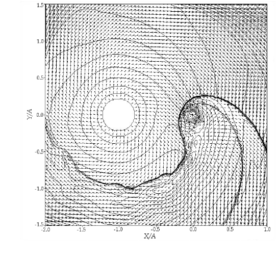
Figure 1: For the paper by Mitsumoto et al. ”3D Gasdynamic Modelling …”

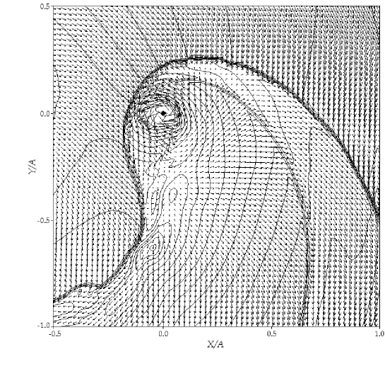
Figure 2: For the paper by Mitsumoto et al. ”3D Gasdynamic Modelling …”

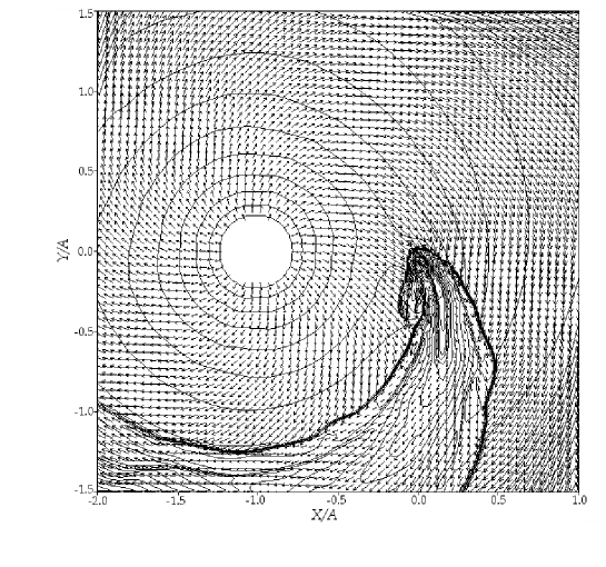
Figure 3: For the paper by Mitsumoto et al. ”3D Gasdynamic Modelling …”

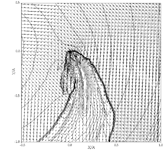
Figure 4: For the paper by Mitsumoto et al. ”3D Gasdynamic Modelling …”

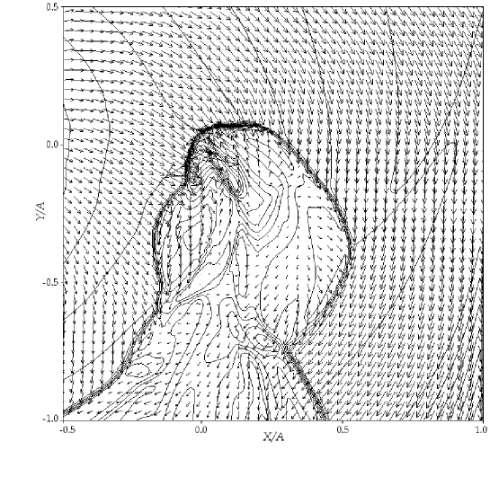
Figure 5: For the paper by Mitsumoto et al. ”3D Gasdynamic Modelling …”

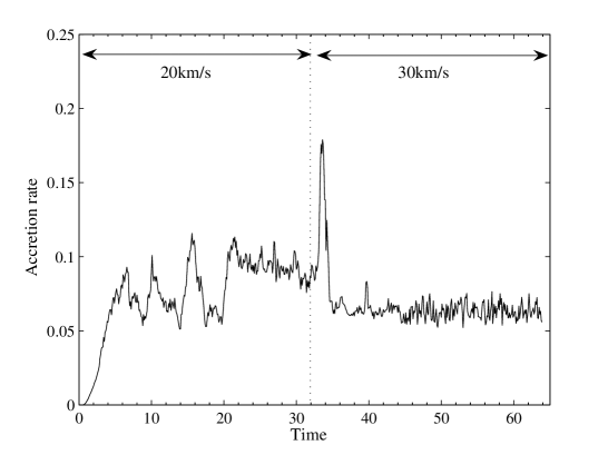
Figure 6: For the paper by Mitsumoto et al. ”3D Gasdynamic Modelling …”

Figure 7: For the paper by Mitsumoto et al. ”3D Gasdynamic Modelling …”