Constraining topology in harmonic space

Abstract

We consider several ways to test for topology directly in harmonic space by comparing the measured $a_{\ell m}$ with the expected correlation matrices. Two tests are of a frequentist nature while we compute the Bayesian evidence as the third test. Using correlation matrices for cubic and slab-space tori, we study how these tests behave as a function of the minimal scale probed and as a function of the size of the universe. We also apply them to different first-year WMAP CMB maps and confirm that the universe is compatible with being infinitely big for the cases considered. We argue that there is an information theoretical limit (given by the Kullback-Leibler divergence) on the size of the topologies that can be detected.

I Introduction

General Relativity has been extremely successful in describing the large-scale features of our universe. But the global shape of space-time is a quantity that is not determined by the local equations of General Relativity. An intriguing possibility is therefore that our universe is much smaller than the size of the particle horizon today.

In the standard model, the universe is described by a Friedmann-Lemaître-Robertson-Walker (FLRW) type metric which is homogeneous and isotropic. If the topology of the universe is not trivial, then we are dealing with a quotient space $X/\Gamma$ where $X$ is one of the usual simply connected FLRW spaces (spherical, Euclidean or hyperbolic) and $\Gamma$ is a discrete and fixed-point free symmetry group that describes the topology. This construction does not affect local physics but changes the boundary conditions (see eg. rep1 ; rep2 and references therein).

This could potentially explain some of the anomalies found in the first-year WMAP data. For example, the perturbations of the cosmic fluids need to be invariant under $\Gamma$. Therefore the largest wavelength of the fluctuations in the CMB cannot exceed the size of the universe, and so the suppression (and maybe the strange alignment) of the lowest CMB multipoles might be due to a non-trivial topology cl1 ; cl2 ; cl3 ; cl4 ; align ; align2 . Additionally, the last scattering surface can wrap around the universe. In this case we receive CMB photons, which originated at the same physical location on the last scattering surface, from different directions. Observationally this would appear as matched (correlated) circles in the CMB circle . An analysis by Cornish et al of the first-year WMAP maps based on a search for matching circles has not found any evidence for a non-trivial topology cornish2 . However, it is difficult to quantify the probability of missing matching circles, and other groups have claimed a tentative detection of circles at scales not probed by Cornish et al (see e.g. roukema ; luminet ). In this paper we study a different approach which can in principle yield both an optimal test as well as a rigorous assessment of the fundamental detection power of the CMB for a cosmic topology.

Instead of working directly with the observed map of CMB temperature fluctuations, we expand the map in terms of spherical harmonics,

$$T(x)=\sum_{\ell,m}a_{\ell m}Y_{\ell m}(x),$$ (1)

where $x$ are the pixels. Both the pixels and the expansion coefficients $a_{\ell m}$ are random variables. In the simplest models of the early universe, they are to a good approximation Gaussian random variables, an assumption that we will make throughout this paper. Their $n$-point correlation functions are then completely determined by the two-point correlation function. The homogeneity and isotropy of the simply-connected FLRW universe additionally requires the two-point correlation of the $a_{\ell m}$ to be diagonal,

$$\langle a_{\ell m}a_{\ell^{\prime}m^{\prime}}^{*}\rangle=C_{\ell}\delta_{\ell\ell^{\prime}}\delta_{mm^{\prime}}.$$ (2)

The symmetry group $\Gamma$ will introduce preferred directions, which will break global isotropy. This in turn induces correlations between off-diagonal elements of the two-point correlation matrix. In this paper we study methods to find such off-diagonal correlations. Such a test is complementary to the matched-circle test of circle ; cornish2 , and if the initial fluctuations are Gaussian then it can use all the information present in the CMB maps and so lead to optimal constraints on the size of the universe. Investigating the amount of information introduced into the two-point correlation matrix by a given topology allows us to decide from an information theoretical standpoint whether the CMB will ever be able to constrain that topology.

We will use the following notation: We often combine the $\ell$ and $m$ indices to a single index $s\equiv\ell(\ell+1)+m$ and mix both notations frequently. The noisy correlation matrix given by the data is ${\cal A}_{ss^{\prime}}\equiv a_{s}a_{s^{\prime}}^{*}$. We will write the correlation matrix which defines a given topology as ${\cal B}_{ss^{\prime}}$. This is the expectation value of the two-point correlation function for $a_{s}$ that describe a universe with that topology.

All the simulations in this paper are based on a flat $\Lambda$CDM model with $\Omega_{\Lambda}=0.7$, a Hubble parameter of $h=0.67$, a Harrison-Zel’dovich initial power spectrum ($n_{S}=1$) and a baryon density of $\Omega_{b}h^{2}=0.019$, as described in riaz1 ; riaz2 . With this choice of cosmological parameters we find a Hubble radius $1/H_{0}\approx 4.8$Gpc while the radius of the particle horizon is $R_{h}\approx 15.6$Gpc. We will denote a toroidal topology as T[X,Y,Z] where X, Y and Z are the sizes of the fundamental domains, in units of the Hubble radius. As an example, T[4,4,4] is a cubic torus of size $(19.3\textrm{Gpc})^{3}$. The volume of such a torus is nearly half that of the observable universe. The diameter of the particle horizon is about $6.5/H_{0}$. But we should note that there are non-zero off-diagonal terms in ${\cal B}_{ss^{\prime}}$ even for universes that are slightly larger than the particle horizon.

We have a range of correlation matrices at our disposal so far. Two of them are cubic tori with sizes $2/H_{0}$ (T[2,2,2]) and $4/H_{0}$ (T[4,4,4]). For these two we have the correlation matrices up to $\ell_{\rm max}=60$ (corresponding to $s_{\rm max}=3720$). We also have two families of slab spaces. The first one, T[X,X,1], has one very small direction of size $1/H_{0}$. The second one, T[15,15,X], has two large directions that are effectively infinite. Both groups include all tori with $X=1,2,\ldots,15$, and we know their correlations matrices up to $\ell_{\rm max}=16$ (or $s_{\rm max}=288$). The correlation matrices analysed in this paper do not contain the integrated Sachs-Wolfe contributions (cf discussion in section VIII.3).

This paper is organised as follows: We start out by matching the measured correlations to a given correlation matrix. We then show that a similar power to distinguish between different correlation matrices can be achieved by using the likelihood. In general we do not know the relative orientation of the map and the correlation matrix, and we discuss how to deal with this issue next. We then present a first set of results from this analysis, before embarking on a simplified analysis of the WMAP CMB data and toroidal topologies.

So far the methods were all of a frequentist nature. Using the likelihood we can also study the evidence for a given topology, which is the Bayesian approach to model selection. We then talk about the issues that we neglected in this paper, and finish with conclusions.

The appendices look in more detail at how the correlation and the likelihood method differ, and how their underlying structure can be used to define “optimal” estimators. We also discuss how selecting an extremum over all orientations can be linked to extreme value distributions, which allows us to derive probability distribution functions that can be fitted to the data for quantifying confidence levels. We finally consider a distance function on covariance matrices, motivated by the Bayesian evidence discussion, and study its application to the comparison between different topologies.

II Detecting Correlations

A priori it is very simple to check whether there are significant off-diagonal terms present in the two-point correlation matrix: One just looks at terms with $\ell\neq\ell^{\prime}$ and/or $m\neq m^{\prime}$. But the variance of the $a_{\ell m}$ is too large as we can observe only a single universe. When computing the $C_{\ell}$ we average over all directions $m$. This averaging then leads to a cosmic variance that behaves like $1/\sqrt{\ell}$. But now we have to consider each element of the correlation matrix separately, leading to a cosmic variance of order $1$ for each element. The matrix is therefore very noisy and we need to “dig out” the topological signal from the noise. Furthermore, if we detect the presence of significant off-diagonal correlations, we still need to verify that they are due to a non-trivial topology and not to some other mechanism that breaks isotropy.

A natural approach to the problem is then to use the expected correlation matrix for a given topology as a kind of filter. To this end we compute a correlation amplitude $\lambda$ which describes how close two matrices are. We do this by minimising

$$\chi^{2}[\lambda]=\sum_{ss^{\prime}}\left({\cal A}_{ss^{\prime}}-\lambda{\cal B}_{ss^{\prime}}\right)^{2}$$ (3)

where ${\cal A}_{ss^{\prime}}=a_{s}a_{s^{\prime}}^{*}$ is the correlation matrix estimated from the data and ${\cal B}_{ss^{\prime}}$ the one which contains the topology that we want to test. For a good fit we expect to find $\lambda\approx 1$ while for a bad fit $\lambda\approx 0$.

We can easily solve $d\chi^{2}/d\lambda=0$ and find that

$$\lambda=\frac{\sum_{ss^{\prime}}{\cal A}_{ss^{\prime}}{\cal B}_{ss^{\prime}}}{\sum_{ss^{\prime}}({\cal B}_{ss^{\prime}})^{2}}$$ (4)

minimises Eq. (3). As we know that we will have to compare our method against maps from an infinite universe with the same power spectrum, we do not sum over the diagonal $s=s^{\prime}$ (which corresponds to $\ell=\ell^{\prime}$ and $m=m^{\prime}$) to improve the signal to noise. This corresponds to replacing the correlation matrix through ${\cal B}\rightarrow{\cal B}-{\cal D}$ where ${\cal D}$ is a diagonal matrix with the power spectrum on the diagonal. If the power spectrum is constant so that ${\cal D}=C\times 1$ then the eigenvectors of the new correlation matrix are the same as those of the original one, and the eigenvalues are replaced by $\epsilon^{(i)}\rightarrow\epsilon^{(i)}-C$. In this case they will no longer be positive.

We could also introduce a covariance matrix in Eq. (3). In the presence of noise this may be useful. In this study we will assume throughout an idealised noise-free and full-sky experiment for simplicity. At any rate the WMAP data will be cosmic variance dominated at the low $\ell$ that we consider here, see section VIII.1. Neglecting the noise contribution, the covariance matrix is $C_{qq^{\prime}}=\langle{\cal B}_{q}{\cal B}_{q^{\prime}}\rangle$ where $q=\{s,s^{\prime}\}$. But as the correlation matrices are already expectation values, we end up with a matrix that has a single non-zero eigenvalue $\epsilon=\sum_{q}{\cal B}_{q}^{2}$. If we invert this singular matrix with the singular value decomposition (SVD) method (setting the inverse of the zero eigenvalues to zero) and minimise the resulting expression for the $\chi^{2}$, we find again Eq. (4).

It is straightforward to compute the expectation value and variance of the $\lambda$ function for two important cases. In the first case the universe is infinite, so that the spherical harmonics $a_{\ell m}$ are characterised by the usual two-point function,

$$\langle a_{\ell m}a_{\ell^{\prime}m^{\prime}}^{*}\rangle_{\infty}=C_{\ell}\delta_{\ell\ell^{\prime}}\delta_{mm^{\prime}}.$$ (5)

In the second case the universe has indeed the topology described by the correlation matrix ${\cal B}$ against which we test the $a_{\ell m}$. In this case the two point function of the spherical harmonics is given by

$$\langle a_{\ell m}a_{\ell^{\prime}m^{\prime}}^{*}\rangle_{\cal B}={\cal B}_{ss^{\prime}}$$ (6)

In both cases the spherical harmonics obey a Gaussian statistics and the higher $n$-point functions are uniquely determined by the two-point function via Wicks theorem.

Let us first define the auto-correlation $U=\sum_{ss^{\prime}}|{\cal B}_{ss^{\prime}}|^{2}$. We remind the reader that such sums in this section exclude the diagonal terms $s=s^{\prime}$ except where specifically mentioned. For an infinite universe, we notice that if we sum only over the non-diagonal elements $s\neq s^{\prime}$ then, since $\langle a_{s}a_{s^{\prime}}^{*}\rangle_{\infty}=C_{s}\delta_{ss^{\prime}}$ the expectation value of lambda is zero, $\langle\lambda\rangle_{\infty}=0$. Else,

$$\langle\lambda\rangle_{\infty}=\frac{1}{U}\sum_{s}C_{s}{\cal B}_{ss}.$$ (7)

If the map was whitened (see below), then $\langle\lambda\rangle_{\infty}={\rm tr}({\cal B})/U$.

For a finite universe,

$$\langle\lambda\rangle_{\cal B}=1$$ (8)

independently if we sum over the diagonal elements or not, as we just recover the auto-correlation in the numerator. Of course the auto-correlation value depends on the summation convention.

For the variance, in the case of an infinite universe, we find

$$\sigma_{\infty}^{2}\equiv\langle\lambda^{2}\rangle_{\infty}-\langle\lambda\rangle_{\infty}^{2}=\frac{2}{U^{2}}\sum_{ss^{\prime}}C_{s}C_{s^{\prime}}|{\cal B}_{ss^{\prime}}|^{2}.$$ (9)

The summation depends again if we keep the diagonal elements or not. For a whitened map, the result simplifies to $\sigma_{\infty}^{2}=2/U$. In a finite universe,

$$\sigma^{2}_{\cal B}=\frac{2}{U^{2}}{\rm tr}\left({\cal B}{\cal B}^{*}{\cal B}{\cal B}^{*}\right),$$ (10)

however now we need to be more careful if we discard the diagonal elements, as then

$$\sigma^{2}_{\cal B}=\frac{2}{U^{2}}\sum_{s1\neq s2,s3\neq s4}\left({\cal B}_{s1s2}{\cal B}^{*}_{s2s3}{\cal B}_{s3s4}{\cal B}^{*}_{s4s1}\right)$$ (11)

Table 1 shows the expectation values of variances for a selection of topologies, computed with these formulas. It may be surprising that the variance of $\lambda$ for an infinite universe depends on the test-topology. However, Eq. (4) depends on ${\cal B}$ even if the $a_{\ell m}$ do not. The variance is a measure of how different ${\cal B}$ is from the diagonal “correlation matrix” of an infinite universe, Eq. (5). The larger the difference, the smaller the variance of $\lambda$, as the random off-diagonal correlations present in the $a_{\ell m}$ are less likely to match those of the test-matrix ${\cal B}$. The value of $\ell_{\rm max}$ in the table was chosen basically arbitrarily, we will discuss later how it influences the measurements. We have also introduced a “signal to noise ratio” S/N which is the difference of the expectation values, divided by the errors added in quadrature,

$$S/N({\cal B},X)=\frac{|\langle X\rangle_{\infty}-\langle X\rangle_{\cal B}|}{\sqrt{\sigma(X)^{2}_{\infty}+\sigma(X)^{2}_{\cal B}}}.$$ (12)

Here $X$ is the estimator used. This gives only a rough indication of the true statistical significance with which a universe with the given topology can be distinguished from an infinite universe. As the distribution of $\lambda$ and $\chi^{2}$ are not exactly Gaussian, S/N is not exactly measured in units of standard deviations. However, it is sufficient to compare the different methods and to illustrate how well different topologies can be detected. For precise statistical results we fit the full distribution, see appendix B.

topology	$\ell_{\rm max}$	$\lambda_{\infty}$	$\lambda_{\cal B}$	S/N [$\sigma$]
T[2,2,2]	60	$0\pm 0.017$	$1\pm 0.102$	$9.7$
T[4,4,4]	60	$0\pm 0.046$	$1\pm 0.082$	$10.6$
T[2,2,2]	16	$0\pm 0.03$	$1\pm 0.34$	$2.9$
T[4,4,4]	16	$0\pm 0.09$	$1\pm 0.22$	$4.2$
T[6,6,1]	16	$0\pm 0.08$	$1\pm 0.33$	$2.9$
T[15,15,6]	16	$0\pm 0.51$	$1\pm 0.59$	$1.3$

Table 1: Comparison of the mean and standard deviation of $\lambda$ for different topologies and different $\ell_{\rm max}$, normalised with the true power spectrum. The S/N value is given by Eq. (12).

The power spectrum $C_{\ell}$ depends of course on the cosmological parameters. To minimise this potential problem we normalise the correlation matrices either by the diagonal $C_{s}\equiv\langle a_{s}a^{*}_{s}\rangle$ or by the usual orientation- averaged power spectrum

$$C_{\ell}=\frac{1}{2\ell+1}\sum_{m}|a_{\ell m}|^{2},$$ (13)

via the prescription

$${\cal B}_{ss^{\prime}}\rightarrow\frac{{\cal B}_{ss^{\prime}}}{\sqrt{C_{s}C_{s^{\prime}}}}.$$ (14)

This is often called “whitening”, and it serves to enforce the same (white noise) power spectrum in both the template and the model being tested. After applying this normalisation the power spectrum is just $C_{s}=1$. We apply the same normalisation to the $a_{\ell m}$. As we will not in general know their “true” input power spectrum, we use the one recovered from the $a_{\ell m}$ themselves. As can be seen in table 2, the division by the recovered power spectrum greatly reduces the variance of $\lambda$ and so improves the detection power for the different topologies. Contrary to table 1 we could not compute the numbers analytically and have estimated them from $10^{4}$ random realisations each of maps with the trivial topology and the ${\cal B}$ topology.

topology	$\ell_{\rm max}$	$\lambda_{\infty}$	$\lambda_{\cal B}$	S/N [$\sigma$]
T[2,2,2]	60	$0\pm 0.015$	$0.973\pm 0.030$	$29.0$
T[4,4,4]	60	$0\pm 0.051$	$0.976\pm 0.044$	$14.5$
T[2,2,2]	16	$0\pm 0.032$	$0.924\pm 0.100$	$8.8$
T[4,4,4]	16	$0\pm 0.091$	$0.948\pm 0.100$	$7.0$
T[6,6,1]	16	$0\pm 0.083$	$0.894\pm 0.200$	$4.1$
T[15,15,6]	16	$0\pm 0.534$	$0.971\pm 0.553$	$1.3$

Table 2: Comparison of the mean and standard deviation of $\lambda$ for different topologies and different $\ell_{\rm max}$, normalised with the power spectrum estimated independently for each realisation. As we see, the signal to noise ratio is improved considerably.

For an infinite universe $C_{s}$ is independent of $m$ and it does not matter whether we divide by $C_{s}$ or $C_{\ell}$. For non-trivial topologies this is not the case as additional correlations are induced in different $m$ modes. For this reason, the division by the $m$-averaged $C_{\ell}$ tends to lead to somewhat stronger constraints. Of course we lose the information encoded in the power spectrum, like the suppression of fluctuations with wavelengths larger than the size of the universe. However, we feel that the improved stability to mis-estimates of the power spectrum and the reduced dependence on the cosmological parameters is worth the trade-off.

The numerical evaluation of Eq. (4) requires a double sum over $s_{\rm max}=\ell_{\rm max}(\ell_{\rm max}+2)$ matrix coefficients. It scales therefore as $\ell_{\rm max}^{4}$. But the correlation matrix of an infinite universe is diagonal, so that we only need to perform a single sum. It should therefore be possible to reduce the work for matrices that are close to being diagonal, ie. for universes with a very large compactification scale. A possibility is to decompose the correlation matrix into a sum over eigenvalues and eigenvectors. We can then only retain the most important eigenvectors. As the correlation matrix is also a covariance matrix, this is somewhat analogous to principal component analysis or the Karhunen-Loeve transform. For a correlation matrix ${\cal B}$ we will write the decomposition as

$${\cal B}_{ss^{\prime}}=\sum_{i}\epsilon^{(i)}v^{(i)}_{s}v^{(i)*}_{s^{\prime}}=\sum_{i}b^{(i)}_{s}b^{(i)*}_{s^{\prime}}.$$ (15)

The $\epsilon^{(i)}$ are the eigenvalues of the matrix ${\cal B}$ and they are real and positive as the matrix is hermitian and positive. This allows us to define effective spherical harmonics $b^{(i)}_{s}\equiv\sqrt{\epsilon^{(i)}}v^{(i)}_{s}$, which have, for example, the same properties under rotation as the usual $a_{\ell m}$.

III Using the likelihood

Instead of considering the correlation between the recovered and the theoretical matrix, we can think of the two-point correlation matrix as the covariance matrix of the $a_{\ell m}$. Then we may ask the question, what is the probability of a covariance matrix ${\cal C}$ given the measured $a_{\ell m}$. This can be answered using Bayesian statistics.

In a first step we need to construct the likelihood function. The probability distribution for a Gaussian random variable $x$ with variance $\sigma^{2}$ and zero expectation value is

$$p(x|\sigma)=\frac{1}{\sqrt{2\pi}\sigma}e^{-\frac{x^{2}}{2\sigma^{2}}}$$ (16)

If we assume that we measure $x$ and want to know $\sigma$, then the likelihood function for finding a certain $x$ is given by ${\cal L}(\sigma)\equiv p(x|\sigma)$. We write the likelihood as a function of the variance, as this is the model parameter that we are interested in.

For many independent variables, the probability distribution is the product, which leads to a sum in the exponent. In the case of the $a_{\ell m}$, the random variables are not independent but are distributed according to a multivariate Gaussian distribution with a covariance matrix ${\cal C}$. The likelihood function then is

$$p(a_{\ell m}|{\cal C})={\cal L}({\cal C})\propto\frac{1}{\sqrt{|{\cal C}|}}\exp\left\{-\frac{1}{2}\sum_{s,s^{\prime}}a^{*}_{s}{\cal C}^{-1}_{ss^{\prime}}a_{s^{\prime}}\right\},$$ (17)

where $|{\cal C}|$ is the determinant of the matrix ${\cal C}$. The covariance matrix is given by the two-point correlation matrix, and $\langle a_{s}\rangle=0$. Any further model assumptions are implicitly included in the choice of ${\cal C}$. Using Bayes law we can invert the probability to find

$$p({\cal C}|a_{\ell m})=\frac{p(a_{\ell m}|{\cal C})p({\cal C})}{p(a_{\ell m})}.$$ (18)

The probability in the denominator is a normalisation constant, while $p({\cal C})$ is the prior probability of a given topology encoded by ${\cal C}$. We will assume that we have no prior information about the topology of the universe, so that this is a constant as well. In this case $p({\cal C}|a_{\ell m})\propto{\cal L}({\cal C})$, ie. we can use the likelihood function to estimate the probability of a topology given a set of $a_{\ell m}$. For our purpose, the covariance matrix is just given by the correlation matrix ${\cal B}$. In general, one may have to add noise to it, and maybe introduce a sky cut.

Generally it is preferable to consider the logarithm of the likelihood, $\log({\cal L})=-1/2(\log(|{\cal B}|)+\chi^{2})+{\rm const.}$ where we have defined

$$\chi^{2}=\sum_{s,s^{\prime}}a^{*}_{s}{\cal B}^{-1}_{ss^{\prime}}a_{s^{\prime}}.$$ (19)

We notice that there is a potential issue with the normalisation of the input model: If $a_{s}\rightarrow 0$ then $\chi^{2}\rightarrow 0$ – generally any model whose $a_{s}$ lead to a bad fit (high $\chi^{2}$) could be renormalised until a reasonable likelihood is obtained. It is therefore required to fix the overall normalisation, and we will do this by using the whitened $a_{s}$, in which case the normalisation is fixed by $\sum_{s}|a_{s}|^{2}=1$.

For the two special cases, the infinite universe and $a_{\ell m}$ distributed according to ${\cal B}$, we can compute expectation value and variance. For the general case we will write $\langle a_{s}a_{s^{\prime}}\rangle={\cal A}_{ss^{\prime}}$. Then

$$\langle\chi^{2}\rangle=\sum_{ss^{\prime}}\langle a_{s}^{*}a_{s^{\prime}}\rangle{\cal B}_{ss^{\prime}}^{-1}={\rm tr}({\cal A}{\cal B}^{-1}),$$ (20)

where we have used the hermeticity of the correlation matrices. The two special cases are

$$\langle\chi^{2}\rangle_{\infty} = \sum_{s}C_{s}{\cal B}_{ss}^{-1}$$ (21)

$$\langle\chi^{2}\rangle_{\cal B} = {\rm tr}(1)=s_{\rm max}$$ (22)

As the $a_{\ell m}$ are Gaussian random variables, we expect to find that $\chi^{2}$ is distributed with a $\chi^{2}$-like distribution. The general expression is rather cumbersome, but for the two special cases we find

$$\sigma^{2}_{\cal B}\equiv\langle(\chi^{2})^{2}\rangle_{\cal B}-\langle\chi^{2}\rangle^{2}_{\cal B}=2s_{\rm max}$$ (23)

and

$$\sigma^{2}_{\infty}=2\sum_{ss^{\prime}}C_{s}C_{s^{\prime}}|{\cal B}^{-1}_{ss^{\prime}}|^{2}.$$ (24)

We list in table 3 some examples, together with the number of standard deviations that the two expectation values lie apart.

topology	$\ell_{\rm max}$	$\chi^{2}_{\infty}$	$\chi^{2}_{\cal B}$	S/N [$\sigma$]
T[2,2,2]	60	$37168\pm 2373$	$3720\pm 86$	$14.1$
T[4,4,4]	60	$14656\pm 1517$	$3720\pm 86$	$7.2$
T[2,2,2]	16	$5608\pm 738$	$288\pm 24$	$7.2$
T[4,4,4]	16	$1802\pm 300$	$288\pm 24$	$5.0$
T[6,6,1]	16	$20781\pm 7103$	$288\pm 24$	$2.9$
T[15,15,6]	16	$309\pm 28$	$288\pm 24$	$0.6$

Table 3: Same as table 1 for $\chi^{2}$.

In these computations, as in the corresponding ones for the correlation coefficient, we have assumed that we normalise the observed $a_{\ell m}$ by the “true” power spectrum (or diagonal). However, we do not know what it is. If we instead normalise them by the estimated one (which is different for each realisation), we change the statistics. It is now no longer Gaussian. Table 4 reproduces the previous one, but now for this scenario. We estimated the numbers from $10^{4}$ numerical realisations for each topology. Again the detection power increases considerably.

topology	$\ell_{\rm max}$	$\chi^{2}_{\infty}$	$\chi^{2}_{\cal B}$	S/N [$\sigma$]
T[2,2,2]	60	$37366\pm 1123$	$4655\pm 438$	$27.1$
T[4,4,4]	60	$14932\pm 1157$	$4027\pm 162$	$9.3$
T[2,2,2]	16	$5690\pm 477$	$474\pm 131$	$10.5$
T[4,4,4]	16	$1841\pm 196$	$335\pm 48$	$7.5$
T[6,6,1]	16	$21093\pm 5645$	$786\pm 557$	$3.6$
T[15,15,6]	16	$309\pm 10$	$289\pm 5$	$1.8$

Table 4: Same as table 2 for $\chi^{2}$.

In appendix A we compare the structure of the correlation estimator to the likelihood $\chi^{2}$. We find that for many cases the $\chi^{2}$ has minimal variance.

IV Rotating the map into position

The situation discussed so far is somewhat misleading: Nature is rather unlikely to align the topology of the universe with our coordinate system. The correlation matrices are not invariant under rotations, as rotations mix $a_{\ell m}$ with different $m$. To parametrise the rotations we use the three Euler angles $\alpha$, $\beta$ and $\gamma$ which describe three subsequent rotations around the $z$, the $y$ and again the $z$ axis. The first and last rotation just lead to a phase change. The rotation around the y-axis couples different $m$ and is given by Wigner rotation matrices $d^{\ell}_{mm^{\prime}}$,

$$a_{\ell m}\rightarrow\sum_{m^{\prime}}e^{-i(m\alpha+m^{\prime}\gamma)}d^{\ell}_{mm^{\prime}}(\beta)a_{\ell m^{\prime}}.$$ (25)

Together, the three rotations can describe any element of the rotation group of order $\ell$. We use the relations given in choi to compute the rotation matrices. Figure 1 shows an example where we plot $\lambda$ while rotating the $a_{\ell m}$ azimuthally. The figure represents the case for $\ell_{\rm max}=60$, for lower values of $\ell_{\rm max}$ the peaks are less sharp and there is less sub-structure. The same is true for the $\chi^{2}$, while the peaks for likelihood, which is proportional to $\exp(-\chi^{2}/2)$, are even much narrower.

Figure 1: Behaviour of the correlation coefficient $\lambda$ under a rotation around the z-axis. The signal is maximal only for very well-defined alignments. We used a T[2,2,2] correlation matrix and $a_{\ell m}$ derived from a T[2,2,2] topology.

We can therefore not avoid probing all possible rotations, either by computing the average or by taking the maximum/minimum of our estimator over all orientations. Possibly the most straightforward approach is to try many random rotations graca . This is simple to program and uses automatically any symmetries present in the template. But due to the precision needed to find the best alignment for some templates, we found that we need in excess of $10^{6}$ rotations to get correct results for $\ell_{\rm max}=60$. We can on the other hand probe systematically all orientations, for example with the total convolution method totconv . In this approach, the rotations with the three Euler angles are replaced by a three-dimensional FFT. This speeds the procedure up a by a large factor. However, we found that we may nonetheless miss the best-fit peaks which can be very sharp (see Figs. 1 and 2).

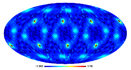
Figure 2: The maximal correlation coefficient for the case of a universe with T[2,2,2] orientation. The sharp, high peaks correspond to the correct orientation of the map with respect to the template.

If we limit ourselves to finding the maximum/minimum efficiently, then we can also start with a random rotation and search for a local extremum nearby. We then repeat the procedure for different random starting locations until we have found a stable global maximum (for example, eight times the same global maximum). This is the safest method, and can be relatively fast depending on the topology.

Computing the average is therefore quite difficult and slow. We also found that using the maximum or minimum results in a much stronger detection than using the average, at least for the $\lambda$ and $\chi^{2}$ estimator. It is possible to improve the average by using the likelihood which is proportional to $\exp(-\chi^{2}/2)$. This decreases the weight of the “wrong” orientations exponentially. However, it makes the average even harder to compute. Furthermore, it lends itself readily to a Bayesian interpretation which is quite different from the frequentist approach followed so far. For this reason we will consider only the maximum/minimum approach here and defer the discussion of the average likelihood to section VII. We also note that it makes no difference if we consider the $\chi^{2}$ estimator or the likelihood when using the extremum over orientations. The exponential function is monotonic and so the maximum or minimum point will not change under it (except that the minimum of the $\chi^{2}$ will turn into a maximum of the likelihood and vice versa). For the same reason, it does not change the statistical weight. If $99$ realisations of model $A$ have a lower $\chi^{2}$ than any of model $B$, then those $99$ realisations will have a higher likelihood as well.

A drawback of using the extremum over all rotations is that we do not know the resulting distribution function. In general we have to compute a large number of test-cases to obtain the distribution, but this is very time-consuming and for high $\ell_{\rm max}$ computing more than a few hundred realisations becomes prohibitive, at least on a single processor. Instead we can find a good approximation to the new distribution by assuming that each rotation leads to a new independent Gaussian distribution. If there are $N$ independent rotations then we need to know the distribution of the maximal value of $N$ draws from a Gaussian distribution. This leads to an extreme value distribution, and exact results are known only for $N<6$. However, for very large $N$, the distribution should converge to one of three limiting cases, analogously to the central limit theorem (see eg. ext_val ). If we fit these distributions to the numerical results then we can obtain confidence limits with a reasonable amount of cpu-time. We discuss this in more detail in appendix B.

topology	$\ell_{\rm max}$	$\chi^{2}_{\infty}$	$\chi^{2}_{\cal B}$	S/N [$\sigma$]
T[2,2,2]	60	$33237\pm 586$	$4588\pm 382$	$41$
T[4,4,4]	60	$11146\pm 438$	$4057\pm 204$	$14$
T[2,2,2]	16	$4062\pm 172$	$469\pm 172$	$17$
T[4,4,4]	16	$1180\pm 73$	$350\pm 47$	$10$
T[6,6,1]	16	$7719\pm 1125$	$675\pm 370$	$6$
T[15,15,6]	16	$287\pm 2.1$	$285\pm 2.5$	$0.6$

Table 5: Comparison of the mean and standard deviation of the $\chi^{2}$ for different topologies and different $\ell_{\rm max}$, normalised with the power spectrum and minimised over rotations.

We compare in tables 5 and 6 the minimal $\chi^{2}$ and maximal $\lambda$ values respectively, taken over all possible orientations. We also quote the resulting S/N value. We notice that especially the $\chi^{2}$ estimator gains in sensitivity. This seems rather surprising, as the distance between the estimator values of an infinite and a finite universe will in general decrease when taking the extremum. However, we also notice that the variance is dramatically decreased, which in turn leads to the even higher detection power.

The reduction of the variance, especially for the infinite universe case, is easy to understand. In table 2 and 4 we use the best-fit alignment for the maps of a finite universe. But the maps with the trivial topology are always randomly aligned (being statistically isotropic). The variance for the infinite universe maps contains therefore an effective “random orientation” contribution. Taking the extremum over all orientations eliminates this contribution. As the infinite universe variance dominates strongly in the case of the $\chi^{2}$ estimator, we find that this estimator benefits more from the reduction of the variance.

topology	$\ell_{\rm max}$	$\lambda_{\infty}$	$\lambda_{\cal B}$	S/N [$\sigma$]
T[2,2,2]	60	$0.08\pm 0.01$	$0.98\pm 0.03$	$28$
T[4,4,4]	60	$0.21\pm 0.02$	$0.98\pm 0.05$	$14$
T[2,2,2]	16	$0.16\pm 0.02$	$0.95\pm 0.08$	$10$
T[4,4,4]	16	$0.38\pm 0.05$	$0.98\pm 0.09$	$6$
T[6,6,1]	16	$0.35\pm 0.05$	$0.94\pm 0.19$	$3$
T[15,15,6]	16	$1.84\pm 0.25$	$1.86\pm 0.27$	$0$

Table 6: Same as table 5 for $\lambda$.

As a final point, we notice that the maximised value of $\lambda$ for the T[15,15,6] topology in table 6 is larger than $1$. This is a sign that we cannot detect that topology. The fluctuations are so large that they completely overwhelm the signal. After maximising over orientations we end up with $\lambda>1$.

V Discussion of general results

V.1 What angular resolution is required?

Is it better to test the maps to arbitrarily high $\ell_{\rm max}$, or to use a lower resolution? One important consideration is the amount of work (and thus of time) needed to evaluate the estimator. For both estimators we need to sum over $s$ and $s^{\prime}$. This means that the required number of operations scales like $\ell_{\rm max}^{4}$. The matrix inversion required for the likelihood evaluation scales like $\ell_{\rm max}^{6}$. However, for two reasons it is normally not the limiting factor. Firstly, as discussed in the previous section, we still need to average over directions. To do that we only need to invert the matrix once at the start, not for every evaluation. But we need to evaluate the likelihood for each orientation, and the number of the required rotations scales roughly like $\ell_{\rm max}^{2}$. We therefore end up with a $\ell_{\rm max}^{6}$ scaling at any rate. Secondly, the most time consuming procedure is the estimation of the variance using simulated maps, and again we only need to invert the matrix once as it stays the same. $\ell_{\rm max}^{6}$ is a rather steep growth, and it is certainly preferable to use the smallest matrices that guarantee a detection.

On the other hand, does the detection always improve with growing $\ell_{\rm max}$? Let us have a look at the correlation estimator, in the case of a whitened map. Clearly $\sigma_{\infty}^{2}=2/U$ can only decrease as long as there are any off-diagonal elements in the correlation matrix. But this is not the dominant error. However, we expect that the main contribution to Eq. (11) is due to the remaining diagonal entries $s_{2}=s_{3}$ and $s_{1}=s_{4}$. This term of the sum is equal to the auto-correlation $U$ and so contributes the same error as $\sigma_{\infty}^{2}$. As the signature of the topology becomes very weak, we expect that the two errors become comparable, but are still decreasing functions of $\ell_{\rm max}$.

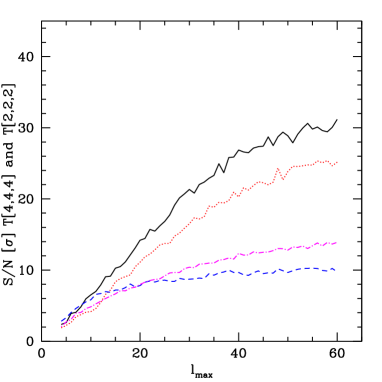
Figure 3: Detection significance assuming that we know the correct orientation. The topologies were T[2,2,2] (solid black and dotted red line) and T[4,4,4] (dashed blue and dot-dashed magenta line). The estimators were respectively the correlation amplitude $\lambda$ (dotted red and dot-dashed magenta line) and the likelihood $\chi^{2}$ (solid black and dashed blue line).

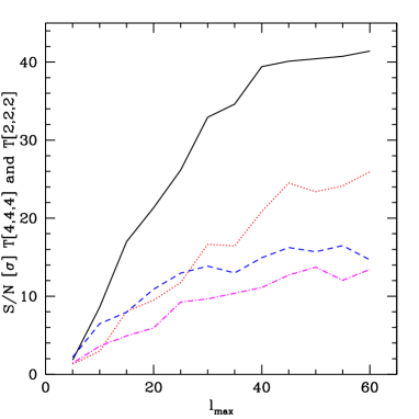
Figure 4: Detection significance when maximising over all orientations. The topologies were T[2,2,2] (solid black and dotted red line) and T[4,4,4] (dashed blue and dot-dashed magenta line). The estimators were respectively the correlation amplitude $\lambda$ (dotted red and dot-dashed magenta line) and the likelihood $\chi^{2}$ (solid black and dashed blue line).

We compare in Figs. 3 and 4 the scaling of $S/N(T[2,2,2])$ and $S/N(T[4,4,4])$ respectively, for the correlation estimator (red dotted / magenta dash-dotted) and the likelihood method (black solid / blue dashed). In all cases we used 100 realisations to compute the average and standard deviation, which explains the noisy curves. As discussed earlier, we find that taking the extremum over rotations can increase the detection power, especially for the $\chi^{2}$ estimator.

We also see that for the T[4,4,4] topology and the correct orientation, the correlation method eventually overtakes the likelihood method. This is most likely because the T[4,4,4] correlation matrix is closer to being diagonal than the T[2,2,2] correlation matrix. At high $\ell$ the diagonal elements start to dominate the contributions to the $\chi^{2}$. The correlator method is not sensitive to this contribution as it does not sum over the diagonal elements. After maximising over orientations, on the other hand, the likelihood is always superior to the correlation method, except maybe for the highest $\ell_{\rm max}$.

We further notice that the detection power keeps increasing with increasing $\ell_{\rm max}$, even though things tend to slow down beyond $\ell\approx 40$. This means that it is useful to consider the largest $\ell$ for which we have the correlation matrix and which we can analyse in a reasonable amount of time. Unfortunately, it is also the case (and hardly surprising) that the smallest universes profit the most from analysing smaller scales. The traces from large but finite universes become rapidly weaker as $\ell_{\rm max}$ increases. As there is little practical difference between a 20 $\sigma$ detection and a 50 $\sigma$ detection, it seems in general quite sufficient to consider scales up to $\ell_{\rm max}=40$ to $60$. The higher $\ell$ may become more important when we also consider the ISW effect.

V.2 What size of the universe can be detected?

From the suppression of the low-$\ell$ modes in the angular power spectrum, the T[4,4,4] topology seems a good candidate for the global shape of the universe. Can we constrain it with one of our methods? Tables 6 and 5 show that we can indeed distinguish a universe with T[4,4,4] topology from an infinite one at over 10 $\sigma$.

As in the previous section we plot in Figs. 5 and 6 the detection significance both before and after maximising over directions. This time we study two families of slab spaces. The first one, T[X,X,1], has one very small direction of size $1/H_{0}$ and we vary the other two. We find that we can clearly detect this kind of topology at $\ell_{\rm max}=16$ for any size of the larger dimensions. For this example-topology it is very striking how the correlation estimator is better if we use the “correct” alignment, while the $\chi^{2}$ becomes more powerful as we extremise over orientations.

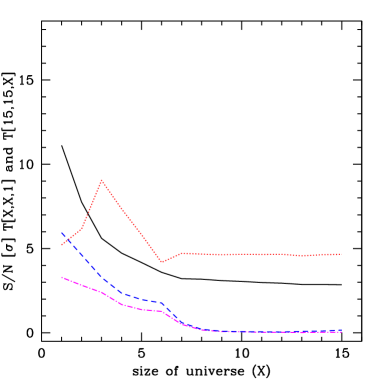
Figure 5: Detection significance assuming that we know the correct orientation. The topologies were T[X,X,1] (solid black and dotted red line) and T[15,15,X] (dashed blue and dot-dashed magenta line). The estimators were respectively the correlation amplitude $\lambda$ (dotted red and dot-dashed magenta line) and the likelihood $\chi^{2}$ (solid black and dashed blue line). We used $\ell_{\rm max}=16$.

The second family, T[15,15,X] is considerably harder to detect as here two directions are very large and effectively infinite. For large values of X we cannot find a difference to an infinite universe. As the third direction shrinks, we start to see differences, but only for $X\leq 3/H_{0}$ can we detect the non-trivial topology at over 2 $\sigma$. In this case the correlation method is always inferior to the $\chi^{2}$. In appendix C we consider a more fundamental distance measure between correlation matrices, namely the Kullback-Leibler divergence. We confirm that we will never be able to distinguish T[15,15,X] with $X>6/H_{0}$ from an infinite universe, see also Fig. 15. This is not very surprising, as in this case the universe is in all directions larger than the particle horizon today.

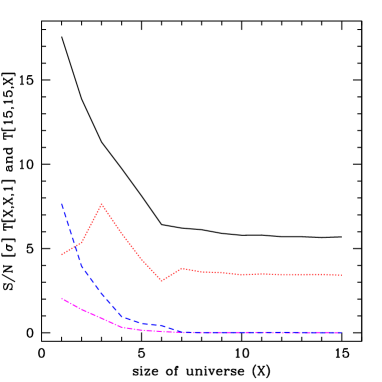
Figure 6: Detection significance when maximising over all orientations. The topologies were T[X,X,1] (solid black and dotted red line) and T[15,15,X] (dashed blue and dot-dashed magenta line). The estimators were respectively the correlation amplitude $\lambda$ (dotted red and dot-dashed magenta line) and the likelihood $\chi^{2}$ (solid black and dashed blue line). Again $\ell_{\rm max}=16$.

VI A simplified analysis of WMAP data

To illustrate the application of these tests to real data, we perform a simplified analysis of the WMAP wmap data. Simplified in the sense that we do not deal with issues like map noise and sky cuts. In general, one has to simulate a large number of maps where both of these effects are included, and which are then analysed with the same pipeline as the actual data map. However, as an illustration we will analyse reconstructed full-sky maps. We use the internal linear combination (ILC) map created by the WMAP team, which we will call the WMAP map from now on. We also use two map reconstructions by by Tegmark, a Wiener filtered map (TW) and a foreground-cleaned map (TC) tegmap . All of these maps are publicly available in HEALPix format healpix with a resolution of $N_{\rm side}=512$. We use this software package to read the map files and to convert them into $a_{\ell m}$.

To get some idea of the systematic errors in this analysis, we additionally analyse the ILC map reconstructed by Eriksen et al. (LILC). They also produced a set of simulated LILC maps (for the trivial topology) with the same pipeline lilc1 ; lilc2 . It is a necessary (but not sufficient) condition to trust our simplified analysis that the results from these maps are consistent with our results for an infinite universe. As an illustration we plot in Fig. 7 the distribution of $\chi^{2}$ for our simple infinite universe maps (black solid histogram) and for the simulated ILC maps which contain noise and foreground contributions (red dashed histogram). We see that the two distributions agree quite well, to within their own variance. The variance observed between the different reconstructed sky maps (WMAP, TC, TW and LILC) is of the same order of magnitude. This example is for T[2,2,2] and $\ell_{\rm max}=16$, but it is representative of the other cases.

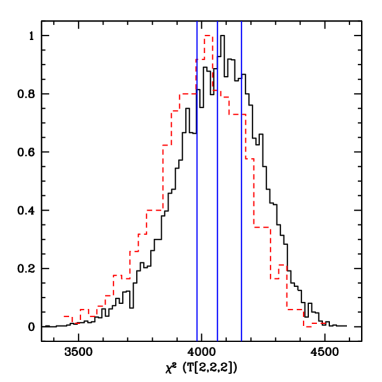
Figure 7: The distribution of the $\langle\chi^{2}\rangle_{\infty}$ estimator values when testing for a T[2,2,2] universe with $\ell_{\rm max}=16$. The black solid histogram is computed from 10000 noiseless full-sky realisations used throughout this paper, while the red dashed histogram used 1000 simulated LILC maps (see text). The vertical lines show the $\chi^{2}$ values of the measured maps, from the left LILC, TW and WMAP (coincident) and TC.

For our standard example, the T[4,4,4] template, we find a maximal value for the 1st year WMAP ILC map of $\lambda_{\rm max}=0.20$. This is about expected for an infinite universe. A universe exhibiting a genuine T[4,4,4] topology should lead to roughly $\lambda_{\rm max}=1$.

topology	$\ell_{\rm max}$	$\chi^{2}$	$P_{\infty}$	$P_{\cal B}$	$\lambda$	$P_{\infty}$	$P_{\cal B}$
T[2,2,2]	60	33130	$0.39$	$0$	0.087	$0.20$	$0$
T[4,4,4]	60	11020	$0.40$	$0$	0.20	$0.64$	$0$
T[6,6,1]	16	8805	$0.85$	$10^{-6}$	0.37	$0.29$	$10^{-5}$
T[15,15,6]	16	290	$0.95$	$0.01$	1.6	$0.16$	$0.84$

Table 7: The value of $\chi^{2}$ and $\lambda$ obtained for the WMAP map, together with the probability of measuring such a value if the universe is infinite ($P_{\infty}$) and if the universe has indeed the topology that we test for ($P_{\cal B}$).

We give in table 7 the values of $\chi^{2}$ and $\lambda$ for the WMAP map. The values for the other maps are not very different. We also give two probabilities for both estimators, $P_{\infty}$ and $P_{\cal B}$. The first one is the probability of measuring a larger value of $\lambda$ (or a smaller value of $\chi^{2}$) if the universe is infinite. $P_{\cal B}$ on the other hand is the probability of measuring a smaller value of $\lambda$ (or a larger value of $\chi^{2}$ if the universe has indeed the topology that we tested for. For a non-detection of any topology we require $P_{\infty}$ to be not too small. A positive detection of a topology on the other hand requires a larger $P_{\cal B}$. If both probabilities are large then we cannot detect that topology (as exemplified eg. for the case of T[15,15,6]). We compute these probabilities with the best-fitting theoretical PDF, as discussed in the appendix B.

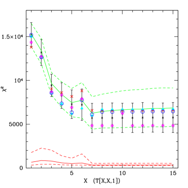
Figure 8: Median and 95% confidence limits as measured with the $\chi^{2}$ estimator for infinite universes (upper green limits) and universes with a T[X,X,1] topology (red lower limits), as a function of size $X$ in units $1/H_{0}$. We also plot the $\chi^{2}$ values of the WMAP map (red crosses), the TW map (cyan triangles) and TC map (blue circles) and the LILC map (magenta stars). All sky maps are consistent with an infinite universe and not consistent with a T[X,X,1] topology for any $X$. We also plot errorbars for the LILC map simulations.

Fig. 8 shows 95% confidence limits (estimated numerically from $10^{4}$ samples) when testing for the presence (red, lower band) or absence (green, upper band) of a T[X,X,1] topology. The WMAP data (points) are all compatible with the infinite universe and rule out this kind of topology very strongly. The bounds from the simulated LILC maps (black error bars) are consistent with our simulated maps with a trivial topology, but systematically a bit lower. We plot the same in Fig. 9 for a T[15,15,X] topology. Again, WMAP is compatible with the infinite universe. But as discussed before, we cannot detect these universes for $X>3/H_{0}$. Overall, all results are consistent with an infinite universe.

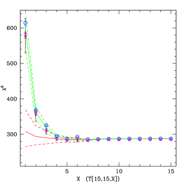
Figure 9: The same as Fig. 8 for the T[15,15,X] topology. Again all WMAP maps are consistent with an infinite universe, but we can only rule out the universes with $X<3$ at more than 95% CL.

VII Bayesian model selection

The likelihood can also be used in a purely Bayesian approach. We are interested in the probability of a model given the data, $p({\cal M}|d)$. If all topologies are taken to be equally probable, then through Bayes theorem the statistical evidence ${\cal E}({\cal M})$ for a model is proportional to the probability of that model, given the data. Using the three Euler angles as parameters $\Theta$, defining the model ${\cal M}$ to be a given topology, and the data $d$ the measured $a_{\ell m}$ we can write the model evidence as

$${\cal E}({\cal M})\propto p(d|{\cal M})=\int\mu(\Theta)\pi(\Theta){\cal L}(\Theta),$$ (26)

where $\pi(\Theta)$ is the prior on the orientation of the map, see eg. mckay . The ratio of the evidence for two topologies is a Bayesian measure of the relative probability. We can think of it as the relative odds of the two topologies. A similar method to constrain the topology was applied previously to the COBE data, see inoue .

The measure $\mu(\Theta)$ on SO(3) needs to be independent of the orientation, which pretty much singles out the Haar measure (up to an irrelevant constant). In terms of the Euler angles it is $d\alpha d\beta d\gamma\sin(\beta)/(8\pi^{2})$ with $\alpha$ and $\gamma$ going from $0$ to $2\pi$, and $\beta$ from $0$ to $\pi$. The volume of SO(3) is then $\int\mu(\Theta)=1$. A simple way to generate random orientations is to select $\alpha$ and $\gamma$ uniformly in $[0,2\pi]$ and $u$ in $[-1,1]$ and then set $\beta=\arccos(u)$.

The advantage of using Bayesian evidence is that it provides a natural probabilistic interpretation which depends only on the actually observed data, but not on simulated data sets. Because of this, there is no need to run large comparison sets. This is a very different view point from the frequentist approach followed so far.

For an infinite universe the correlation matrix is diagonal and rotationally invariant (due to isotropy). The integral over the alignment becomes trivial in this case. If we use whitening then the correlation matrix is just the unit matrix and we have

$$\chi^{2}=\sum_{s}|a_{s}|^{2}=s_{\rm max}.$$ (27)

The second equality is due to the whitening. The likelihood is then

$${\cal L}_{\infty}=\frac{{\rm const}}{|1|^{1/2}}e^{-1/2\chi^{2}(\theta)}={\rm const}\,e^{-s_{\rm max}/2},$$ (28)

where the constant normalisation is independent of the topology. We will neglect it as it drops out when comparing the evidence for different models. This “infinite” evidence gives us a reference point, with our choice of measure on SO(3) and of normalisation it is

$$-\log({\cal E}_{\infty})=\frac{s_{\rm max}}{2}.$$ (29)

On the other hand, if the universe is infinite then we know that the expected $\chi^{2}$ is the trace of the inverse of the correlation matrix that we test for. It is again rotationally invariant as $\langle a_{s}a_{s^{\prime}}^{*}\rangle$ is rotationally invariant. The log-evidence is on average

$$-\log({\cal E})=\frac{1}{2}\left({\rm tr}({\cal B}^{-1})+\log|{\cal B}|\right).$$ (30)

We notice that the expected log-evidence difference to the true infinite universe is the Kullback-Leibler divergence,

$$\Delta\log({\cal E})=D_{KL}(1||{\cal B})=\frac{1}{2}\left(\log|{\cal B}|+{\rm tr}({\cal B}^{-1}-1)\right)$$ (31)

We should not forget though that this is a very crude approximation to the evidence. Nonetheless, Eq. (31) gives a useful indication of the odds that we can detect a given topology, as it can be evaluated very rapidly, without performing the integration over orientations. Fundamentally, this is the amount of additional information about topology contained in the correlation matrix ${\cal B}$. If the amount of information is not sufficient to distinguish it from an infinite universe, no test will ever be able to tell the two apart. We discuss the Kullback-Leibler (KL) divergence and its possible applications in more detail in appendix C.

Of course, faced with real data we have to evaluate the actual evidence integral. Unfortunately the likelihood is extremely strongly peaked around the correct alignments (especially for a non-trivial topology), and it is very difficult to sample from it. Already the $\lambda$ and $\chi^{2}$ estimators require a very precise alignment to reach the true maximum or minimum. Exponentiating $-\chi^{2}$ leads to much narrower peaks in the extrema, and makes the problem far worse. In Fig. 10 we plot the relative likelihood (normalised to unity at the peak) for a universe with T[4,4,4] topology close to a correct alignment (the vertical line), and for different $\ell_{\rm max}$. The broadest peak corresponds to $\ell_{\rm max}=16$, and we added the location of $10^{4}$ points evenly spaced between $0$ and $2\pi$ as black crosses. This corresponds to a total of roughly $10^{11}$ points to cover all of SO(3). For $\ell_{\rm max}=16$ we could get away with using only every 10th point (about $10^{8}$ points in total) and still detect the high-likelihood region. But not so for $\ell_{\rm max}=32$ and $60$ (the narrower peaks), which would easily be missed.

This renders methods like thermodynamic integration infeasible. On the other hand, we are dealing only with three parameters. Direct integration is therefore marginally possible by using an adaptive algorithm. For $\ell_{\rm max}=16$ we need to start out with at least $10^{6}$ points in order to detect the high-probability regions at all. This means that we have to count on $10^{7}$ to $10^{8}$ likelihood evaluations. The situation gets worse for higher resolution maps, as both the likelihood evaluations require more time and the high-probability regions shrink. We therefore only quote results for $\ell_{\rm max}=8$ in this section.

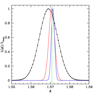
Figure 10: Relative likelihood for a T[4,4,4] topology around one of the symmetry points where a simulated T[4,4,4] map aligns correctly. The broadest (black) curve is for $\ell_{\rm max}=16$, the intermediate (red) curve $\ell_{\rm max}=32$ and the narrowest (blue) curve $\ell_{\rm max}=60$. The vertical green line lies at $\phi=\pi/2$. The crosses show the location of $10^{4}$ points between $\phi=0$ and $\phi=2\pi$.

topology	$\ell_{\rm max}$	WMAP	TC	TW	LILC	$D_{KL}(1||{\cal B})$
$\infty$	8	$-17$	$-17$	$-17$	$-17$	0
T[2,2,2]	8	$-114$	$-103$	$-100$	$-102$	172
T[4,4,4]	8	$-46$	$-41$	$-47$	$-44$	64
T[6,6,1]	8	$-526$	$-\infty$	$-\infty$	$-\infty$	1733
T[15,15,6]	8	$-17$	$-18$	$-18$	$-17$	1

Table 8: The log-evidence $\log_{10}({\cal E})$ for a range of topologies and data maps (see text). We also quote the KL divergence with respect to an infinite universe for comparison.

As the data sets which define our likelihood we use the same four maps as in the frequentist analysis: The ILC map by the WMAP team (WMAP), two maps by Tegmark et al, the Wiener filtered map (TW) and the foreground- cleaned map (TC) and the ILC map by Eriksen et al. (LILC). We quote the logarithm (to base 10) of the evidence in table 8 for our usual range of example models. The relevant quantity for model comparison is the difference of these values (corresponding to the ratio of the probability). If the log evidence of a model $A$ is 3 higher than the log evidence of model $B$, we conclude that the odds for model $A$ are $10^{3}$ times better. This can be seen as fairly good odds in favour of model $A$. We plot in Fig. 14 the correspondence between the logarithm of a probability ratio and the number of standard deviations ($\sigma$) for a Gaussian random variable.

All topologies except T[15,15,6] are excluded at high confidence. The evidence values for the different reconstructed CMB maps agree at least qualitatively. We plot in Fig. 11 the evidence of the T[15,15,X] cases as a function of X. The two smallest universes are strongly excluded, $X=2$ could be excluded if we used a higher resolution, and the rest are too close to the infinite universe to be constrained. We also plot the mean and standard deviation of the simulated LILC maps as error bars. The T[X,X,1] cases are all so completely excluded that the integral is just barely feasible given the huge numbers involved.

We would like to remind the reader that the results in this section are always relative to the observed map. It is therefore a bit worrying that the evidences differ by several orders of magnitude when we consider the different full-sky reconstructions. We also checked the stability of the results for 1000 simulation of the LILC map with known (trivial) topology. We found it to be rather poor (cf the large error bars in fig 11), although this may be partially due to the smaller range of $\ell$. Another possible source for this lack of stability is our simplistic likelihood. The Bayesian interpretation of the results is only true if we are able to derive the correct likelihood. This is an important difference to the frequentist results where we calibrate the statistical interpretation with the comparison sets. In the frequentist scenario, we may end up with a sub-optimal test, but we will not get wrong results if we use the wrong likelihood function. Not so in the Bayesian case, which forces us to be more careful. A possible way out is to reconstruct a likelihood from the set of simulated LILC maps.

Normally, a difference of $2$ to $3$ in $\log_{10}({\cal E})$ is taken to be sufficient to strongly disfavour a model against another one. This may be reasonable for a full analysis that takes into account all the issues discussed in the following section. For full-sky reconstructed maps we feel that we should require at least a difference of $10$. Overall it seems that the frequentist approach leads to results which are more stable against the uncertainties introduced by the full-sky reconstruction and foreground removal.

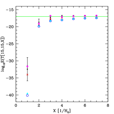
Figure 11: The evidence of a T[15,15,X] topology with $\ell_{\rm max}=8$ for four different full-sky reconstructions of the WMAP data (WMAP red crosses, TW cyan triangle, TC blue circle and LILC magenta stars). The black error bars are derived from simulated LILC maps. They are consistent with the actual LILC data map. The green line shows the predicted evidence of an infinite universe.

VIII Cosmic Complications

This paper aims at introducing and discussing the different methods for constraining the topology of the universe in harmonic space. In doing so we study an idealised situation with perfect data, neglecting several issues that are present in the real world. Here we give a quick overview over the main complications that will have to be dealt with for a rigorous analysis. Clearly they will change the quantitative results presented here, but we do not expect that they will lead to qualitative changes in the results.

VIII.1 Noise

If we assume constant and independent per-pixel noise $\sigma_{N}$ then the covariance matrix of the $a_{\ell m}$ acquires an additional diagonal term,

$$\langle a_{s}^{*}a_{s^{\prime}}\rangle+\sigma_{N}^{2}\delta_{ss^{\prime}}.$$ (32)

This is fairly close to what many CMB experiments (like WMAP and Planck) expect for their data. The CMB power spectrum on large scales behaves roughly like $1/\ell^{2}$ (Harrison-Zel’dovich) with a power of about $C_{10}\approx 60\mu{\rm K}^{2}$. For any experiment that probes scales beyond the first peak, we can conclude that the large scales ($\ell<100$ say) are completely signal dominated. Taking WMAP as an example, we see that Fig. 1 of wmap_hinshaw gives a noise contribution to the $C_{\ell}$ of $0.1$ to $0.6\mu{\rm K}^{2}$ depending on the assembly. As the noise additionally (to first order) does not enter in the off-diagonal terms, we can safely neglect it for a first analysis.

More generally we expect a fixed noise variance per detector and per observation. The resulting per-pixel noise is $\sigma_{N}(x)=\sigma_{0}/\sqrt{N_{\rm obs}}$. Turning again to WMAP as an example, we find that they cite a noise variance $\sigma_{0}\approx 2-7$ mK. Expressed in terms of the spherical harmonic coefficients, the correlation matrix in this scenario becomes

$$\langle a_{s}^{*}a_{s^{\prime}}\rangle+\sigma_{0}^{2}\int d^{2}\!xN_{\rm obs}^{-1}(x)Y^{*}_{s}(x)Y_{s^{\prime}}(x)$$ (33)

where the integration runs over all pixels $x$. Because of its spatial variation, the noise is no longer confined to the diagonal and should strictly speaking be taken into account. But the off-diagonal terms will still be very small. The most straightforward way to include the noise is to simulate maps with the correct power spectrum and noise properties and to co-add them. This is especially the case when we deal with a complicated sky cut (see below).

The ILC maps that we used here have more complicated noise properties due to the full-sky reconstruction. But the noise itself will still be negligible on large scales, compared to the signal. More worrying are potential foreground contaminations that were not completely subtracted. We explore that problem partially in section VI by using simulated LILC maps.

VIII.2 Uncertainties in the cosmological parameters

So far we have used correlation matrices computed for a fixed cosmological model. But there are still significant uncertainties present in the true value of the cosmological parameters, and even in the underlying cosmological model. An example was recently discussed in params . In principle we have to take such uncertainties into account. For the Bayesian model selection approach, we could do it straight-forwardly by marginalising over them. Of course this may mean computing a large number of correlation matrices for different cosmological models, which would lead to a computational challenge. Alternatively, one should consider a selection of models and incorporate the variance of the correlations into a systematic error on the correlation matrices.

In practise, we hope that the whitening which eliminates differences in the power spectrum will also minimise the effects due to this parameter uncertainty. At the very least it will do so for the “infinite universe” tests where no off-diagonal correlations are present. The result that the full-sky WMAP maps are compatible with an infinite universe is thus not affected by the parameter uncertainty.

VIII.3 The integrated Sachs-Wolfe effect

An issue somewhat related to the last point is that not all perturbations are generated on the last scattering surface. Some of them are due to the integrated Sachs-Wolfe (ISW) effect. Especially perturbations due to the late ISW effect that are generated relatively close to us are then not affected by the global topology and carry no information about it. They act as a kind of noise for our purposes. This contribution is especially problematic when searching for matching circles in pixel space. It is readily included when working with the correlation matrices, even though it will also be subject to the parameter uncertainties and it will lower our detection power substantially.

The rapid decrease of the late ISW effect with increasing $\ell$ provides an additional incentive for probing smaller scales, $\ell\approx 40-60$.

VIII.4 Sky cuts

Here we have only considered full-sky maps. Unfortunately a large part of the sky-sphere is covered by our galaxy which leads to foregrounds that are not easy to subtract and obscure the true CMB signal. The most conservative approach is therefore to remove a part of the sky via a sky cut. This amounts to introducing a mask ${\cal M}(x)$ in pixel space, with value $1$ on the pixels $x$ where the CMB signal is clean, and $0$ in the contaminated parts of the sky. We then consider the pseudo-$a_{\ell m}$

$$\hat{a}_{\ell m}=\int d^{2}\!x{\cal M}(x)\delta T(x)Y_{\ell m}(x)$$ (34)

instead of the true $a_{\ell m}$. We can perform the masking operation directly in harmonic space, using the spherical Fourier transform of the mask,

$${\cal M}_{ss^{\prime}}=\int d^{2}\!x{\cal M}(x)Y_{s}(x)Y^{*}_{s^{\prime}}(x).$$ (35)

The relation between the true $a_{\ell m}$ and the observed pseudo-$a_{\ell m}$ is then given by $\hat{a}_{s}=\sum_{s^{\prime}}{\cal M}_{ss^{\prime}}a_{s^{\prime}}$. Unfortunately the mask matrix ${\cal M}$ corresponds to a loss of information and can in general not be inverted. We could of course use SVD to invert it, and eliminate the small SVD eigenvalues. However, this would be quite similar to a full-sky reconstruction. Instead, it may be preferable to apply the sky cut to the correlation matrix as well. The resulting pseudo-correlation matrix is then

$$\hat{{\cal B}}={\cal M}^{{\dagger}}{\cal B}{\cal M}.$$ (36)

This leads to two problems. The first one is purely computational: The sky cut has a fixed orientation (with respect to the $a_{\ell m}$). So far it did not matter if we rotated the correlation matrix or the $a_{\ell m}$, as only the relative orientation counted. But since the sky cut defines an absolute orientation we now need to apply the rotation to the correlation matrix. Rotating the correlation matrix is considerably more costly than rotating the observed $a_{\ell m}$. The use of the eigenvector decomposition (15) and rotation of the effective spherical harmonics $b_{\ell m}$ can somewhat alleviate the situation if only a few eigenvalues dominate the sum.

The second problem is that a sky cut and its associated mask matrix introduce just the kind of correlations between different $a_{\ell m}$ that we are looking for. A sky cut will impact significantly on our ability to constrain large universes. We will have to either accept this limitation, or hope that better full-sky reconstruction and component separation methods (for example comp_sep ) will become available. However, one would have to demonstrate that such methods do indeed not change the correlation properties of the $a_{\ell m}$ in a way that influences the detection of a topology-signature. At the very least one has to consider such effects as systematic errors and include them in the error budget of a full analysis.

IX Conclusions and outlook

In this paper we have studied three ways to constrain the topology of our universe directly with the correlation matrix of the $a_{\ell m}$. If the primordial fluctuations are Gaussian then these correlation matrices contain all the information about the global shape of our universe that is carried by the CMB. By trying to find their traces in the measured $a_{\ell m}$ we can construct the most sensitive probes possible.

We studied two frequentist estimators, $\lambda$ which describes the correlation amplitude between the theoretical correlation matrix ${\cal B}$ and the measured $a_{\ell m}$, and $\chi^{2}=a^{\dagger}{\cal B}^{-1}a$. Although $\lambda$ has certain advantages at high $\ell$ by leaving out the diagonal terms, we found the $\chi^{2}$ to be generally superior after taking into account the random orientation of the observed map. We also computed the Bayesian evidence, which we found to be a very sensitive probe. But the angular integration is computationally very intensive, especially at high resolutions. Additionally, much care is needed in constructing the likelihood function. For these reasons, the $\chi^{2}$ minimised over rotations seems the most useful of our tests.

For our scenario we find that even high multipoles, $\ell>50$, still carry important information about the topology. However, the amount of work needed to extract the information scales as a high power of $\ell$. For most cases $\ell\approx 30-40$ seems a sufficient upper limit.

We finally apply our methods to a set of reconstructed full-sky maps based on WMAP data. For all topologies considered (cubic and slab tori) we find no hints of a non-trivial topology. Based on the exclusion of the T[4,4,4] topology, we conclude that the fundamental domain is at last $19.3\textrm{Gpc}$ long if it is cubic. We rule out (not very surprisingly) any universe where a fundamental domain in any direction is smaller than $4.8$Gpc (based on the T[X,X,1] cases). If the universe is infinite in two directions, then the third direction has to be larger than $14.4$Gpc. These limits still allow two copies of the universe inside the current particle horizon. We prefer to understand this analysis as a demonstration of our methods, as we neglected a range of important issues such as the ISW effect.

The noise of the WMAP data is already cosmic variance dominated on the scales of interest. Future experiments will not be able to provide significantly better CMB temperature data sets, although some improvement may come from better foreground separation with more frequencies, and from e.g. using polarisation maps in addition to the temperature maps. Short of waiting a few billion years for the universe to expand further, these tests and especially the information theoretical limits provided by the Kullback-Leibler divergence give us an idea about what we can learn of the shape of our universe.

Appendix A Finding an optimal estimator

It is interesting to compare the expressions for the $\chi^{2}$ and the $\lambda$ estimator. The philosophy of the two approaches is very different. In the first case we write down a likelihood function for a given covariance matrix. In the second case we correlate the noisy estimated covariance matrix with a theoretical model. We then use the correlation amplitude $\lambda$ as a measure of goodness-of-fit. To compare the two methods, we use the eigen-space expansion (15). As ${\cal B}$ is hermitian, the eigenvalues are real; if we use the full covariance matrix, which is positive definite, the eigenvalues are also positive.

Introducing this expansion into the expression for $\chi^{2}$ we find

$$\chi^{2}=\sum_{i}\frac{1}{\epsilon^{(i)}}\left|\sum_{s}a_{s}v_{s}^{(i)}\right|^{2}.$$ (37)

To compute the same for the correlation amplitude, we use that the eigenvectors are normalised and orthogonal, $\sum_{s}v_{s}^{(i)}v_{s}^{(j)*}=\delta_{ij}$. The autocorrelation is then simply $\sum_{ss^{\prime}}|{\cal B}_{ss^{\prime}}|^{2}=\sum_{i}\epsilon^{(i)2}$ and the correlation amplitude is

$$\lambda=\frac{\sum_{i}\epsilon^{(i)}\left|\sum_{s}a_{s}v_{s}^{(i)}\right|^{2}}{\sum_{i}\left(\epsilon^{(i)}\right)^{2}}.$$ (38)

If one eigenvalue dominates, then the two expressions coincide. If all eigenvalues are equal, then $\chi^{2}=s_{\rm max}\lambda$. This happens for an infinite universe if we normalise it by the power spectrum. In both cases the statistical properties are equal.

In the intermediate cases we see that both correspond to a different weighting of the correlations between the eigenvectors and the $a_{\ell m}$. The question arising now is whether we can determine an optimal weighting that leads to the smallest variance if the $a_{\ell m}$ are drawn either from an infinite universe or from one with covariance matrix ${\cal B}$. If the two requirements are not the same, it is preferable to optimise with respect to the infinite universe, as large universes will be close to this case.

Let us, as an example and guided by the above discussion, postulate a general estimator

$$\alpha=\sum_{i}\alpha^{(i)}X_{i}$$ (39)

where we use the structure that we observed above,

$$X_{i}=\left|\sum_{s}a_{s}v_{s}^{(i)}\right|^{2}.$$ (40)

The expectation value and the variance of the general estimator are

$$\langle\alpha\rangle = \sum_{i}\alpha^{(i)}\langle X_{i}\rangle$$ (41)

$$\sigma^{2} \equiv \langle\alpha^{2}\rangle-\langle\alpha\rangle^{2}$$ (42)

$$= \sum_{i,j}\alpha^{(i)}\alpha^{(j)}\left(\langle X_{i}X_{j}\rangle-\langle X_{i}\rangle\langle X_{j}\rangle\right)$$

The aim is to find the $\alpha^{(i)}$ that minimise the variance of the estimator, subject to a normalisation constraint. We are going to consider several different limits. The simplest example is the case where the eigenvectors are due to an infinite universe, in which case $v_{s}^{(i)}=\delta_{is}$. It is now easy to see that $\langle X_{i}\rangle=\langle a_{i}a_{i}^{*}\rangle=C_{i}$ and $\langle X_{i}X_{j}\rangle=C_{i}C_{j}+2|{\cal A}_{ij}|^{2}$ where ${\cal A}_{ij}$ is the covariance matrix from which the observed $a_{\ell m}$ are drawn. The expectation value and variance of the general estimator are now

$$\langle\alpha\rangle = \sum_{i}\alpha^{(i)}C_{i}$$ (43)

$$\langle\alpha^{2}\rangle-\langle\alpha\rangle^{2} = 2\sum_{ij}\alpha^{(i)}\alpha^{(j)}|{\cal A}_{ij}|^{2}$$ (44)

Adding the constraint $\sum_{i}\alpha^{(i)}=s_{\rm max}$ with a Lagrange multiplier $l$ we have to minimise the expression

$$2\sum_{ij}\alpha^{(i)}\alpha^{(j)}|{\cal A}_{ij}|^{2}+l\left(\sum_{i}\alpha^{(i)}-s_{\rm max}\right).$$ (45)

The relevant system of equations is found as usual by computing the first derivatives with respect to $l$ and the coefficients and setting them to zero to find the extrema:

$$\sum_{i}\alpha^{(i)} = s_{\rm max}$$ (46)

$$l+4\sum_{i}\alpha^{(i)}|{\cal A}_{ik}|^{2} = 0\quad\forall k=1,\ldots,s_{\rm max}$$ (47)

This is a linear system which can be solved via matrix inversion. For the simplest case where ${\cal A}_{ij}=C_{i}\delta_{ij}$ (the observed $a_{\ell m}$ are also drawn from an infinite universe with power spectrum $C_{i}$) we can write down the solution up to a normalisation constant:

$$\alpha^{(i)}\propto\frac{1}{C_{i}}$$ (48)

We assume that both the template and sky have the same power spectrum $C_{i}$. In our case this also means that the eigenvalues of ${\cal A}$ are $\epsilon^{(i)}=C_{i}$. The minimum variance estimator is therefore proportional to the $\chi^{2}$. On the other hand, after whitening $C_{i}=1$ and both estimators become equivalent.

It is also easy to consider the case when the $a_{s}$ are distributed according to the same correlation matrix ${\cal B}$ that we compare them with. As the eigenvectors are orthonormal, we find that

$$\langle X_{i}\rangle_{\cal B} = \epsilon^{(i)}$$ (49)

$$\langle X_{i}X_{j}\rangle_{\cal B} = \epsilon^{(i)}\epsilon^{(j)}+2(\epsilon^{(i)})^{2}\delta_{ij}$$ (50)

The variance of the estimator is then

$$\sigma_{\alpha}^{2}=2\sum_{i}\alpha_{i}^{2}(\epsilon^{(i)})^{2}.$$ (51)

This is minimised by

$$\alpha_{i}\propto\frac{1}{\epsilon^{(i)}}$$ (52)

as before. The $\chi^{2}$ estimator has therefore the minimal variance in this case as well.

However, we see from tables 3 and 4 that the dominant error is not $\langle\rangle_{\cal B}$ but $\langle\rangle_{\infty}$. We should therefore try to minimise this variance instead. Here the $a_{\ell m}$ are those of an infinite universe while the eigenvectors are those of the correlation matrix ${\cal B}$. It is possible to derive an optimal estimator for this case, but it is rather unwieldy.

Finally, our aim is to maximise the detection of a given topology. This is not necessarily the same as minimising the variance as discussed above. Firstly, the discussion necessarily disregards the deviations introduced by dividing the $a_{\ell m}$ by their own power spectrum. Secondly, the $\lambda$ correlation estimator gains power by leaving out the diagonal terms. And thirdly, we use the extremum over all orientations which will also change the results.

Appendix B Extreme value distributions

Computing the extrema of the estimators for a large number of cases takes a lot of cpu time. It is important to use this information efficiently, for example by fitting a theoretically motivated distribution function. We try to derive such a fitting distribution by considering all rotations as independent random realisations. We then use the maximum or minimum, depending on the estimator. This is known as extreme value statistics ext_val . For example in the case of $\lambda$ we found that its distribution is nearly Gaussian. We find with our approximations for the distribution of the maximum out of $n$ draws

$$C_{n}(z) = p\left[\text{max}(\lambda_{1},\ldots,\lambda_{n})\leq z\right]$$ (53)

$$= p(\lambda_{1}\leq z,\ldots,\lambda_{n}\leq z)$$ (54)

$$= \prod_{i=1}^{n}p(\lambda_{i}\leq z)$$ (55)

$$= C(z)^{n}.$$ (56)

Here $C(z)=(1+\text{erf}(\sqrt{2}z))/2$ is the cumulative probability function of a single univariate Gaussian random variable and $C_{n}(z)$ the same for the maximum of $n$ independent univariate Gaussians. The median lies at $C_{n}(z)=1/2$ or $C(z)=2^{-1/n}$. We show in figure 12 the location of the median as a function of $n$. For the relevant number of independent rotations, we find a shift of $4$ to $6$ sigma.

Figure 12: The location of the median value in number of standard deviations $\sigma$ for the maximum value out of $n$ Gaussian random variables.

A theorem similar to the central limit theorem says that there are certain limiting distributions to which the distribution of an extremal value converges. The limiting distribution for an unbounded variable like $\lambda$ is the Gumbel distribution, with a probability distribution function (PDF) of the form

$$P(x)=\exp(-z-\exp(-z))/\sigma\quad{\rm where~{}}z=(x-\mu)/\sigma$$ (57)

(see e.g. coles for a discussion and another astrophysical application). The expectation value is $\sigma\gamma+\mu$ and the variance is $\sigma^{2}\pi^{2}/6$ where $\gamma\approx 0.577$ is the Euler constant. We can use these two values to find $\sigma$ and $\mu$ given the variance and expectation value of the distribution.

The cumulative distribution function (CDF) is

$$F(x)=e^{-\exp(-z)},$$ (58)

We can consider e.g. $F(x=0.95)$ as two-sigma upper limit. We find that for $N$ of the order of a few thousand, $5\sigma$ is a very conservative upper bound. Even though the extreme value distribution moves the expectation values up or down, the variances around those values can still remain surprisingly small. The signal to noise ratio need not decrease because of the shift. Indeed, as discussed in V we find that it often even increases.

For a bounded variable like a $\chi^{2}$ the situation is similar, except that the limiting distribution is now called Weibull distribution, with

$$P(x)=\frac{\gamma}{x}\left(\frac{x}{\alpha}\right)^{\gamma}\exp\left\{-\left(\frac{x}{\alpha}\right)^{\gamma}\right\}.$$ (59)

The two parameters $\alpha$ and $\gamma$ can be fixed again by measuring the expectation value $\mu=\alpha\Gamma[1+1/\gamma]$ and variance $\sigma^{2}=\alpha^{2}(\Gamma[1+2/\gamma]-\Gamma[1+1/\gamma]^{2})$ of the numerical distribution. The CDF is simply

$$F(x)=1-e^{-(t/\alpha)^{\gamma}},$$ (60)

and $x\geq 0$.

However, we found that this form is a bad fit even to just the minimum over independent variables with a true $\chi^{2}$ type distribution. It seems better to allow for two different exponents, leading to a PDF of the form

$$P(x)=\frac{\gamma}{\alpha\Gamma[(1+\beta)/\gamma]}\left(\frac{x}{\alpha}\right)^{\beta}\exp\left\{-\left(\frac{x}{\alpha}\right)^{\gamma}\right\}.$$ (61)

We call this the extended Weibull distribution. The CDF is now

$$F(x)=1-\frac{\Gamma[(1+\beta)/\gamma,(x/\alpha)^{\gamma}]}{\Gamma[(1+\beta)/\gamma]}$$ (62)

where $\Gamma[a,b]$ is the incomplete Gamma function, with $\Gamma[a,0]=\Gamma[a]$ and $\Gamma[1,x]=\exp(-x)$. We recover the standard case for $\beta=\gamma-1$. We found the extended Weibull distribution to be the best-fitting distribution in general, even for the $\lambda$ estimator. Figure 13 shows an example fit to the PDF of $\lambda$ for a T[6,6,1] distribution.

There are different ways to fit the theoretical extreme value distribution to the numerical CDF. We could for example maximise the Kolmogorov-Smirnov probability. Instead we decided to use a Bayesian approach: We consider the numerical values as “data points” $d_{i}$ for the true CDF and use the theoretical distribution as a model with parameters $\theta_{j}$. For each data point the probability is then given by $p(d_{i}|\theta)=F(d_{i})$. As all the data points are independent, we can define a likelihood function ${\cal L}$ as

$$\chi^{2} \equiv -2\log({\cal L}(\theta))$$ (63)

$$= -2\log\left(\prod_{i}F(d_{i})\right)$$ (64)

$$= -2\sum_{i}\log\left(F(d_{i})\right).$$ (65)

We can then easily compute the posterior probability of the parameters $\theta$ that describe the distribution with a Markov-chain Monte Carlo method.

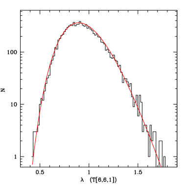
Figure 13: The PDF of $\lambda$ for a T[6,6,1] topology maximised over rotations (black histogram, $10^{4}$ samples) and the best fit using an extended Weibull distribution (red curve). The Kolmogorov-Smirnov probability of the fit is 42%.

Appendix C A distance between topologies

C.1 The Kullback-Leibler divergence

Let us consider the following question: What is the expectation value of the ratio of the likelihoods for covariance matrices ${\cal A}$ and ${\cal B}$ if the $a_{s}$ are distributed according to a correlation matrix ${\cal A}$? We have already computed the log-likelihood in section III, the first case is simply

$$\langle\log{\cal L}\rangle=-\frac{1}{2}\left(\log|{\cal A}|+{\rm tr}(1)\right).$$ (66)

and the second one

$$\langle\log{\cal L}\rangle=-\frac{1}{2}\left(\log|{\cal B}|+{\rm tr}({\cal A}{\cal B}^{-1})\right)$$ (67)

The difference between the two expressions is the logarithm of the likelihood ratio,

$$\langle\Delta\log{\cal L}\rangle=-\frac{1}{2}\left(\log|{\cal A}|-\log|{\cal B}|+{\rm tr}(1-{\cal B}^{-1}{\cal A})\right)$$ (68)

This is precisely the Kullback-Leibler divergence between the two Gaussian distributions described by ${\cal A}$ and ${\cal B}$.

topology	$\ell_{\rm max}$	${\rm tr}({\cal B}^{-1})$	$\log(|{\cal B}|)$	$D_{KL}(1||{\cal B})$
$\infty$	16	288	0	0
T[2,2,2]	16	4661	-486	1944
T[4,4,4]	16	1570	-192	545
T[15,15,6]	16	309	-8	6
T[6,6,1]	16	20781	-399	10047

Table 9: Some key quantities for computing the KL divergence. The whitening enforces ${\rm tr}({\cal B})=s_{\rm max}(=288)$.

The Kullback-Leibler (KL) divergence is in general defined for two probability distributions $p$ and $q$ as

$$D_{KL}(p||q)\equiv\int p\log\left(\frac{p}{q}\right).$$ (69)

Notice that this is not symmetric, so the symmetrised form $D(p||q)+D(q||p)$ is sometimes used if it is not clear which distribution is the fundamental one. In information theory the KL divergence describes the relative entropy (or information) between the two probability distributions $p$ and $q$. This corresponds for example to the amount of information wasted when trying to describe data distributed as $q$ with a model based on $p$ (see e.g. mckay ).

We consider the KL divergence for random variables $x$ which have a normal distribution with zero mean and covariance matrix ${\cal A}$,

$$p({\cal A},x)=(2\pi)^{n/2}|{\cal A}|^{-1/2}\exp\left(-\frac{1}{2}x^{T}{\cal A}^{-1}x\right).$$ (70)

We can derive an expression for the KL divergence directly in terms of the covariance matrices by evaluating the Gaussian integrals:

$$\int p({\cal A})\log\frac{p({\cal A})}{p({\cal B})}=\frac{1}{2}\left(\log|{\cal B}|-\log|{\cal A}|-tr\left[1-{\cal B}^{-1}{\cal A}\right]\right).$$ (71)

This is the same expression as Eq. (68).

We have encountered the KL divergence in section VII where we used it as a zeroth order approximation to the evidence. In general, it is not rotationally invariant. But although we cannot use it directly, we can define a distance between two topologies if their correlation matrices are aligned along the same symmetry axes. $D_{KL}({\cal A}||{\cal B})$ corresponds then to the maximal signal that we can expect. The base of the logarithm that we use corresponds to a choice of units – in information theory the conventional choice is base 2, corresponding to bits. We quote the numerical results to base 10, as it makes it easy to interpret the result: if $D_{KL}({\cal A}||{\cal B})=3$ then we can (at best!) expect to distinguish the topologies at the 1000:1 level. If $D_{KL}({\cal A}||{\cal B})\leq 2$ then it will be very difficult to distinguish the two topologies. Of course the Kullback-Leibler divergence depends also on the resolution, $\ell_{\rm max}$.

When comparing to results quoted as number of standard deviations, we use that for a Gaussian random variable

$$P(|x|>\nu\sigma)=1-\sqrt{\frac{2}{\pi}}\int_{\nu}^{\infty}e^{-x^{2}/2}dx=1-{\rm erf}(\nu/\sqrt{2})$$ (72)

For $x\gg 1$ we can well approximate $1-{\rm erf}(x)$ by $\exp(-x^{2})/(\sqrt{\pi}x)$. In figure 14 we plot $\log_{10}(P(|x|>\nu\sigma))$ against $\nu\sigma$ to make it easy to compare the two quantities.

Figure 14: The probability that a Gaussian random variable is more than $n$ standard deviations away from the mean. This figure helps to compare the results expressed in number of $\sigma$ with those expressed as $\log_{10}(P)$.

C.2 Information theoretical limits on detecting a topology

As we have already mention often, a FLRW universe with the trivial topology is homogeneous and isotropic. Correspondingly its correlation matrix is rotationally invariant. In this special case also the KL divergence does not depend on the relative orientation of the two universes. The quantity $D_{KL}(1||{\cal A})$ measures therefore directly how much “information” separates the universe with the topology described by ${\cal A}$ from an infinitely large universe. If there is not enough information, then we will never be able to detect that topology.

Figure 15 shows the KL divergence between an infinite universe and a T[15,15,X] topology for different $X=L/H_{0}$ and $\ell_{\rm max}$. We see that the distance falls rapidly for $L>6/H_{0}$. Even increasing $\ell_{\rm max}$ does not help as the correlation matrices become essentially identical. Hence, even though we can still detect correlations in spite of this universe being larger than the particle horizon in all directions, we will not be able to distinguish it from an infinite universe at a significant level.

Figure 15: The Kullback-Leibler divergence $D_{KL}(1||T[15,15,X])$ between an infinite universe and a slab-space, as a function of the size of the smallest dimension $X$. We show curves for $\ell_{\rm max}=8$, $12$ and $16$. For $X>3$ the topology becomes difficult to detect and for $X>6$ it is basically impossible for any $\ell_{\rm max}$. Compare with Fig. 6.

C.3 Comparing different templates

If the topology of the universe is non-trivial then we will end up using different correlation matrices until one fits. If a template is completely wrong we expect to see no signal at all. However, if the template belongs to a topology which is “similar” to the real one, then we may find a reduced signal.

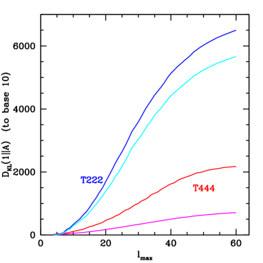
Figure 16: The scaling of the Kullback-Leibler divergence as function of $\ell_{\rm max}$. The curves show $D_{KL}(1||T[2,2,2])$ (blue) and $D_{KL}(1||T[4,4,4])$ (red). Both keep increasing for the whole range of $\ell_{\rm max}$ considered, showing that there is information on these topologies even at relatively small scales. We also plot $D_{KL}(T[4,4,4]||T[2,2,2])$ (cyan) and $D_{KL}(T[2,2,2]||T[4,4,4])$. We argue that the smallness of the latter curve shows that it is possible to detect a T[2,2,2] universe with a T[4,4,4] template.

What does similar mean in this context? As an example, let’s assume that either the universe has a T[2,2,2] topology while we test with T[4,4,4] or the opposite. In the first case, the signal is actually too strong, and we end up finding a correlation of order unity ($\lambda=0.91\pm 0.05$), but we pay the price of too much noise. If we had used the T[2,2,2] template, our detection would have been more significant. On the other hand, if we use the T[2,2,2] template for a T[4,4,4] universe then the correlation is smaller ($\lambda=0.11\pm 0.02$) while the (non-maximised) value for infinite universes is $\lambda=0\pm 0.02$. Overall, it seems better to test first the largest universe that can still be distinguished from an infinite one.

This is also borne out by the Kullback-Leibler divergence between T[4,4,4] and T[2,2,2], shown in Fig. 16. We find for example with $\ell_{\rm max}=16$ that $D_{KL}(T[4,4,4]||T[2,2,2])\approx 2000$ while $D_{KL}(T[2,2,2]||T[4,4,4])=265$. Both are smaller than $D_{KL}(1||T[2,2,2])$ and the latter is smaller than $D_{KL}(1||T[4,4,4])$, indicating that it is possible to detect a $T[2,2,2]$ universe with a $T[4,4,4]$ template. Another possible use of the Kullback-Leibler divergence is therefore to map out the space of topologies and to identify those which are very similar. This helps to reduce the space of models that needs to be searched.

References

- (1) M. Lachièze-Rey and J.-P. Luminet, Phys. Rep. 254, 135 (1995).
- (2) J. Levin, Phys. Rep. 365, 251 (2002).
- (3) I.Yu. Sokolov, JETP Lett. 57, 617 (1993).
- (4) A.A. Starobinsky, JETP Lett. 57, 622 (1993).
- (5) D. Stevens, D. Scott and J. Silk, Phys. Rev. Lett. 71, 20 (1993).
- (6) A. de Oliveira-Costa and G.F. Smoot, Astrophys. J. 448, 477 (1995).
- (7) W.S. Hipólito-Ricaldi and G.I. Gomero, astro-ph/0507238 (2005).
- (8) J.G. Cresswell et al., astro-ph/0512017 (2005).
- (9) N.J. Cornish, D. Spergel and G. Starkmann, Class. Quantum Grav. 15, 2657 (1998).
- (10) N.J. Cornish et al., Phys. Rev. Lett. 92, 201302 (2004).
- (11) B. Roukema et al, Astron. Astrophys. 423, 821 (2004).
- (12) J.-P. Luminet, Phys. World 18, 22 (2005), archived under physics/0509171.
- (13) A. Riazuelo et al., Phys. Rev. D 69, 103514 (2004).
- (14) A. Riazuelo et al., Phys. Rev. D 69, 103518 (2004).
- (15) C.H. Choi et al., J. Chem. Phys. 111, 8825 (1999).
- (16) P. Dineen, G. Rocha and P. Coles, MNRAS 358, 1285 (2005).
- (17) B.D. Wandelt and K.M. Górski, Phys. Rev. D 63, 123002 (2001).
- (18) E.W. Weisstein, “Extreme Value Distribution”, from MathWorld, http://mathworld.wolfram.com/ExtremeValueDistribution.html
- (19) C.L. Bennett et al., ApJS 148, 97 (2003).
- (20) M. Tegmark, A. de Oliveira-Costa and A. Hamilton, Phys. Rev. D 68 123523 (2003).
- (21) K.M. Górski, E. Hivon and B.D. Wandelt, astro-ph/9812350; http://www.eso.org/science/healpix/
- (22) H.K. Eriksen et al., astro-ph/0508196 (2005).
- (23) H.K. Eriksen et al., ApJ 612, 633 (2004).
- (24) D.J.C. MacKay, Information Theory, Inference, and Learning Algorithms, Cambridge University Press (2003).
- (25) K.T. Inoue and N. Sugiyama, Phys. Rev. D 67, 043003 (2003).
- (26) G. Hinshaw et al., ApJS 148, 135 (2003).
- (27) M. Makler, B. Mota and M.J. Reboucas, astro-ph/0507116 (2005).
- (28) H.K. Eriksen et al., astro-ph/0508268 (2005).
- (29) P. Coles, MNRAS 231, 125 (1988).