An analysis of ultraviolet spectra of Extreme Helium Stars and new clues to their origins

Abstract

Abundances of about 18 elements including the heavy elements Y and Zr are determined from $Hubble$ $Space$ $Telescope$ Space Telescope Imaging Spectrograph ultraviolet spectra of seven extreme helium stars (EHes): LSE 78, BD +10^∘ 2179, V1920 Cyg, HD 124448, PV Tel, LS IV-1^∘ 2, and FQ Aqr. New optical spectra of the three stars – BD +10^∘ 2179, V1920 Cyg, and HD 124448 – were analysed, and published line lists of LSE 78, HD 124448, and PV Tel were analysed afresh. The abundance analyses is done using LTE line formation and LTE model atmospheres especially constructed for these EHe stars. The stellar parameters derived from an EHe’s UV spectrum are in satisfactory agreement with those derived from its optical spectrum. Adopted abundances for the seven EHes are from a combination of the UV and optical analyses. Published results for an additional ten EHes provide abundances obtained in a nearly uniform manner for a total of 17 EHes, the largest sample on record.

The initial metallicity of an EHe is indicated by the abundance of elements from Al to Ni; Fe is adopted to be the representative of initial metallicity. Iron abundances range from approximately solar to about one-hundredth of solar. Clues to EHe evolution are contained within the H, He, C, N, O, Y, and Zr abundances. Two novel results are (i) the O abundance for some stars is close to the predicted initial abundance yet the N abundance indicates almost complete conversion of initial C, N, and O to N by the CNO-cycles; (ii) three of the seven stars with UV spectra show a strong enhancement of Y and Zr attributable to an $s$-process.

The observed compositions are discussed in light of expectations from accretion of a He white dwarf by a CO white dwarf. Qualitative agreement seems likely except that a problem may be presented by those stars in which the O abundance is close to the initial O abundance.

1 Introduction

The extreme helium stars whose chemical compositions are the subject of this paper are a rare class of peculiar stars. There are about 21 known EHes. They are supergiants with effective temperatures in the range 9000 – 35,000 K and in which surface hydrogen is effectively a trace element, being underabundant by a factor of 10,000 or more. Helium is the most abundant element. Carbon is often the second most abundant element with C/He $\simeq$ 0.01, by number. Nitrogen is overabundant with respect to that expected for the EHe’s metallicity. Oxygen abundance varies from star to star but C/O $\simeq$ 1 by number is the maximum ratio found in some examples. Abundance analyses of varying degrees of completeness have been reported for a majority of the known EHes. The chemical composition should be a primary constraint on theoretical interpretations of the origin and evolution of EHes.

Abundance analyses were first reported by Hill (1965) for three EHes by a curve-of-growth technique. Model atmosphere based analyses of the same three EHes were subsequently reported by Schönberner & Wolf (1974), Heber (1983) and Schönberner (1986). Jeffery (1996) summarized the available results for about 11 EHes. More recent work includes that by Harrison & Jeffery (1997), Jeffery & Harrison (1997), Drilling, Jeffery, & Heber (1998), Jeffery (1998), Jeffery et al. (1998), Jeffery, Hill & Heber (1999), and Pandey et al. (2001). Rao (2005a) reviews the results available for all these stars.

In broad terms, the chemical compositions suggest a hydrogen deficient atmosphere now composed of material exposed to both H-burning and He-burning. However, the coincidence of H-processed and He-processed material at the stellar surface presented a puzzle for many years. Following the elimination of several proposals, two principal theories emerged: the ‘double-degenerate’ (DD) model and the ‘final-flash’ (FF) model.

The ‘double-degenerate’ (DD) model was proposed by Webbink (1984) and Iben & Tutukov (1984) and involves merger of a He white dwarf with a more massive C-O white dwarf following the decay of their orbit. The binary began life as a close pair of normal main sequence stars which through two episodes of mass transfer evolved to a He and C-O white dwarf. Emission of gravitational radiation leads to orbital decay and to a merger of the less massive helium white dwarf with its companion. As a result of the merger the helium white dwarf is destroyed and forms a thick disk around the more massive C-O companion. The merging process lasting a few minutes is completed as the thick disk is accreted by the C-O white dwarf. If the mass of the former C-O white dwarf remains below the Chandrasekhar limit, accretion ignites the base of the accreted envelope forcing the envelope to expand to supergiant dimensions. Subsequently, it will appear probably first as a cool hydrogen-deficient carbon star (HdC) or a R Coronae Borealis star (RCB). As this H-deficient supergiant contracts, it will become an EHe before cooling to become a single white dwarf. (If the merger increases the C-O white dwarf’s mass over the Chandrasekhar limit, explosion as a SN Ia or formation of a neutron star occurs.)

Originally described in quite general terms (Webbink, 1984; Iben & Tutukov, 1984), detailed evolution models were computed only recently (Saio & Jeffery 2002). The latter included predictions of the surface abundances of hydrogen, helium, carbon, nitrogen and oxygen of the resultant EHe. A comparison between predictions of the DD model and observations of EHe’s with respect to luminosity to mass ratios ($L/M$), evolutionary contraction rates, pulsation masses, surface abundances of H, C, N, and O, and the number of EHes in the Galaxy concluded that the DD model was the preferred origin for the EHes and, probably, for the majority of RCBs. The chemical similarity and the commonality of $L/M$ ratios had long suggested an evolutionary connection between the EHes and the RCBs (Schönberner, 1977; Rao, 2005a).

Saio & Jeffery’s (2002) models do not consider the chemical structure of the white dwarfs and the EHe beyond the principal elements (H, He, C, N and O), nor do they compute the full hydrodynamics of the merger process and any attendant nucleosynthesis. Hydrodynamic simulations have been addressed by inter alia Hachisu, Eriguchi & Nomoto (1986), Benz et al. (1990), Segretain, Chabrier & Mochkovitch (1997), and Guerrero, García-Berro & Isern (2004). Few of the considered cases involved a He and a C-O white dwarf. In one example described by Guerrero et al., a 0.4$M_{\odot}$ He white dwarf merged with a 0.6$M_{\odot}$ C-O white dwarf with negligible mass loss over the 10 minutes required for complete acquisition of the He white dwarf by the C-O white dwarf. Accreted material was heated sufficiently that nuclear burning occurs, mostly by ¹²C$(\alpha,\gamma)^{16}$O, but is quickly quenched. It would appear that negligible nucleosynthesis occurs in the few minutes that elapse during the merging.

The second model, the FF model, refers to a late or final He-shell flash in a post-AGB star which may account for some EHes and RCBs. In this model (Iben et al., 1983), the ignition of the helium shell in a post-AGB star, say, a cooling white dwarf, results in what is known as a late or very late thermal pulse (Herwig, 2001). The outer layers expand rapidly to giant dimensions. If the hydrogen in the envelope is consumed by H-burning, the giant becomes a H-deficient supergiant and then contracts to become an EHe. The FF model accounts well for several unusual objects including, for example, FG Sge (Herbig & Boyarchuk, 1968; Langer, Kraft & Anderson, 1974; Gonzalez et al., 1998) and V4334 Sgr (Sakurai’s object) (Duerbeck & Benetti, 1996; Asplund et al., 1997b), hot Wolf-Rayet central stars, and the very hot PG1159 stars (Werner, Heber & Hunger, 1991; Leuenhagen, Hamann & Jeffery, 1996).

Determination of surface compositions of EHes should be rendered as complete as possible: many elements and many stars. Here, a step is taken toward a more complete specification of the composition of seven EHes. The primary motivation of our project was to establish the abundances of key elements heavier than iron in order to measure the $s$-process concentrations. These elements are unobservable in the optical spectrum of a hot EHe but tests showed a few elements should be detectable in ultraviolet spectra. A successful pilot study of two EHes with the prime motive to measure specifically the abundances of key elements heavier than iron was reported earlier (Pandey et al., 2004). We now extend the study to all seven stars and to all the elements with useful absorption lines in the observed UV spectral regions. In the following sections, we describe the ultraviolet and optical spectra, the model atmospheres and the abundance analysis, and discuss the derived chemical compositions in light of the DD model.

2 Observations

A primary selection criterion for inclusion of an EHe in our program was its UV flux because useful lines of the heavy elements lie in the UV. Seven EHes were observed with the Hubble Space Telescope and the Space Telescope Imaging Spectrometer (STIS). The log of the observations is provided in Table 1. Spectra were acquired with STIS using the E230M grating and the $0.^{"}2\times 0.^{"}06$ aperture. The spectra cover the range from 1840 Å to 2670 Å at a resolving power ($R=\lambda/\Delta\lambda$) of 30,000. The raw recorded spectra were reduced using the standard STIS pipeline. A final spectrum for each EHe was obtained by co-addition of two or three individual spectra. Spectra of each EHe in the intervals 2654 Å to 2671 Å and 2401 Å to 2417 Å illustrate the quality and diversity of the spectra (Figures 1 and 2), principally the increasing strength and number of absorption lines with decreasing effective temperature.

New optical spectra of BD +10^∘ 2179, and V1920 Cyg were acquired with the W.J. McDonald Observatory’s 2.7-m Harlan J. Smith telescope and the coudé cross-dispersed echelle spectrograph (Tull et al., 1995) at resolving powers of 45,000 to 60,000. The observing procedure and wavelength coverage were described by Pandey et al. (2001).

Finally, a spectrum of HD 124448 was obtained with the Vainu Bappu Telescope of the Indian Institute of Astrophysics with a fiber-fed cross-dispersed echelle spectrograph (Rao et al., 2004, 2005b). The 1000Å of spectrum in 50Å intervals of 30 echelle orders from 5200 Å to nearly 10,000 Å was recorded on a Pixellant CCD. The resolving power was about 30,000. The S/N in the continuum was 50 to 60.

Figure 1: A sample of the STIS spectra of the seven EHes. The spectra are normalized to the continuum and are shown with offsets of about 0.5 between each. Several lines are identified in this window from 2654 Å to 2671 Å. Stars are arranged from top to bottom in order of decreasing effective temperature.

Figure 2: A sample of the STIS spectra of the seven EHes. The spectra are normalized to the continuum and are shown with offsets of about 0.5 between each. Several lines are identified in this window from 2401 Å to 2417 Å. Stars are arranged from top to bottom in order of decreasing effective temperature.

Table 1: The $HST$ $STIS$ Observations

Star	$V$	Obs. Date	Exp. time	S/N	Data Set Name
	mag		s	at 2500Å
V2244 Oph	11.0			28
($=$LS IV-1∘ 2)		7 Sep 2002	1742		O6MB04010
		7 Sep 2002	5798		O6MB04020
BD+1∘ 4381	9.6			59
($=$FQ Aqr)		10 Sep 2002	1822		O6MB07010
		10 Sep 2002	5798		O6MB07020
HD 225642	10.3			45
($=$V1920 Cyg)		18 Oct 2002	1844		O6MB06010
		18 Oct 2002	2945		O6MB06020
BD +10∘ 2179	10.0			90
		14 Jan 2003	1822		O6MB01010
		14 Jan 2003	2899		O6MB01020
CoD -46∘ 11775	11.2			50
($=$LSE 78)		21 Mar 2003	2269		O6MB03010
		21 Mar 2003	2269		O6MB03020
HD 168476	9.3			90
($=$PV Tel)		16 Jul 2003	2058		O6MB05010
		16 Jul 2003	3135		O6MB05020
HD 124448	10.0			70
		21 Jul 2003	1977		O6MB05010
		21 Jul 2003	3054		O6MB05020

3 Abundance Analysis – Method

3.1 Outline of the procedure

The abundance analysis follows closely a procedure described by Pandey et al. (2001, 2004). H-deficient model atmospheres have been computed using the code STERNE (Jeffery, Woolf & Pollacco, 2001) for the six stars with an effective temperature greater than 10,000 K. For FQ Aqr with $T_{\rm eff}=8750$ K, we adopt the Uppsala model atmospheres (Asplund et al., 1997a). Both codes include line blanketing. Descriptions of the line blanketing and the sources of continuous opacity are given in the above references. Pandey et al. (2001) showed that the two codes gave consistent abundances at 9000 – 9500 K, the upper temperature bound for the Uppsala models and the lower temperature bound for STERNE models. Local thermodynamic equilibrium (LTE) is adopted for all aspects of model construction.

A model atmosphere is used with the Armagh LTE code SPECTRUM (Jeffery, Woolf & Pollacco, 2001) to compute the equivalent width of a line or a synthetic spectrum for a selected spectral window. In matching a synthetic spectrum to an observed spectrum we include broadening due to the instrumental profile, the microturbulent velocity $\xi$ and assign all additional broadening, if any, to rotational broadening. In the latter case, we use the standard rotational broadening function $V(v\sin i,\beta)$ (Unsöld, 1955; Dufton, 1972) with the limb darkening coefficient set at $\beta=1.5$. Observed unblended line profiles are used to obtain the projected rotational velocity $v\sin i$. We find that the synthetic line profile, including the broadening due to instrumental profile, for the adopted model atmosphere ($T_{\rm eff}$,$\log g,\xi$) and the abundance is sharper than the observed. This extra broadening in the observed profile is attributed to rotational broadening. Since we assume that macroturbulence is vanishingly small, the $v\sin i$ value is an upper limit to the true value.

The adopted $gf$-values are from the NIST database, Wiese, Fuhr & Deters (1996), Ekberg (1997), Uylings & Raassen (1997), Raassen & Uylings (1997), Martin, Fuhr & Wiese (1988), Artru et al. (1981), Crespo Lopez-Urrutia et al. (1994), Salih, Lawler & Whaling (1985), Kurucz’s database, and the compilations by R. E. Luck (private communication). The adopted $gf$-values for Y iii, Zr iii, La iii, Ce iii, and Nd iii, are discussed in Pandey et al. (2004). The Stark broadening and radiative broadening coefficients, if available, are mostly taken from the Vienna Atomic Line Database. The data for computing He i profiles are the same as in Jeffery, Woolf & Pollacco (2001), except for the He i line at 6678Å, for which the $gf$-values and electron broadening coefficients are from Kurucz’s database. The line broadening coefficients are not available for the He i line at 2652.8Å. Detailed line lists used in our analyses are available in electronic form.

3.2 Atmospheric parameters

The model atmospheres are characterized by the effective temperature, the surface gravity, and the chemical composition. A complete iteration on chemical composition was not undertaken, i.e., the input composition was not fully consistent with the composition derived from the spectrum with that model. Iteration was done for the He and C abundances which, most especially He, dominate the continuous opacity at optical and UV wavelengths. Iteration was not done for the elements (e.g., Fe – see Figures 1 and 2) which contribute to the line blanketing.

The stellar parameters are determined from the line spectrum. The microturbulent velocity $\xi$ (in km s^-1) is first determined by the usual requirement that the abundance from a set of lines of the same ion be independent of a line’s equivalent width. The result will be insensitive to the assumed effective temperature provided that the lines span only a small range in excitation potential. For an element represented in the spectrum by two or more ions, imposition of ionization equilibrium (i.e., the same abundance is required from lines of different stages of ionization) defines a locus in the ($T_{\rm eff},\log g)$ plane. Except for the coolest star in our sample (FQ Aqr), a locus is insensitive to the input C/He ratio of the model. Different pairs of ions of a common element provide loci of very similar slope in the ($T_{\rm eff},\log g)$ plane.

An indicator yielding a locus with a contrasting slope in the ($T_{\rm eff},\log g)$ plane is required to break the degeneracy presented by ionization equilibria. A potential indicator is a He i line. For stars hotter than about 10,000 K, the He i lines are less sensitive to $T_{\rm eff}$ than to $\log g$ on account of pressure broadening due to the quadratic Stark effect. The diffuse series lines are, in particular, useful because they are less sensitive to the microturbulent velocity than the sharp lines. A second indicator may be available: species represented by lines spanning a range in excitation potential may serve as a thermometer measuring $T_{\rm eff}$ with a weak dependence on $\log g$.

For each of the seven stars, a published abundance analysis gave estimates of the atmospheric parameters. We took these estimates as initial values for the analysis of our spectra.

4 Abundance Analysis – Results

The seven stars are discussed one by one from hottest to coolest. Inspection of Figures 1 and 2 shows that many lines are resolved and only slightly blended in the hottest four stars. The coolest three stars are rich in lines and spectrum synthesis is a necessity in determining the abundances of many elements.

The hotter stars of our sample have a well defined continuum, the region of the spectrum (having maximum flux) free of absorption lines is treated as the continuum point and a smooth curve passing through these points (free of absorption lines) is defined as the continuum. For the relatively less hot stars of our sample, same procedure as above is applied to place the continuum; for the regions which are severely crowded by absorption lines, the continuum of the hot stars is used as a guide to place the continuum in these crowded regions of the spectra. These continuum normalised observed spectra are also compared with the synthetic spectra to judge the continuum of severely crowded regions. However, extremely crowded regions for e.g., of FQ Aqr are not used for abundance analysis.

Our ultraviolet analysis is mainly by spectrum synthesis, but, we do measure equivalent widths of unblended lines to get hold of the microturbulent velocity. However, the individual lines from an ion which contribute significantly to the line’s equivalent width ($W_{\lambda}$) are synthesized including the adopted mean abundances of the minor blending lines. The abundances derived, including the predicted $W_{\lambda}$ for these derived abundances, for the best overall fit to the observed line profile are in the detailed line list, except for most of the optical lines which have the measured equivalent widths. Discussion of the UV spectrum is followed by comparisons with the abundances derived from the optical spectrum and the presentation of adopted set of abundances. Detailed line lists (see for SAMPLE Table 2 which lists some lines of BD +10^∘ 2179) used in our analyses lists the line’s lower excitation potential ($\chi$), $gf$-value, log of Stark damping constant/electron number density ($\Gamma_{el}$), log of radiative damping constant ($\Gamma_{rad}$), and the abundance derived from each line for the adopted model atmosphere. Also listed are the equivalent widths ($W_{\lambda}$) corresponding to the abundances derived by spectrum synthesis for most individual lines. The derived stellar parameters of the adopted model atmosphere are accurate to typically: $\Delta$$T_{\rm eff}$ = $\pm$500 K, $\Delta$$\log g$ = $\pm$0.25 cgs and $\Delta$$\xi$ = $\pm$1 km $s^{-1}$. The abundance error due to the uncertainty in $T_{\rm eff}$ is estimated by taking a difference in abundances derived from the adopted model ($T_{\rm eff}$,$\log g,\xi$) and a model ($T_{\rm eff}$$+$500 K,$\log g,\xi$). Similarly, the abundance error due to the uncertainty in $\log g$ is estimated by taking a difference in abundances derived from the adopted model ($T_{\rm eff}$,$\log g,\xi$) and a model ($T_{\rm eff}$,$\log g+0.25,\xi$). The rms error in the derived abundances from each species for our sample due to the uncertainty in $T_{\rm eff}$ and $\log g$ of the derived stellar parameters are in the detailed line lists. The abundance errors due to the uncertainty in $\xi$ are not significant, except for some cases where the abundance is based on one or a few strong lines and no weak lines, when compared to that due to uncertainties in $T_{\rm eff}$ and $\log g$. These detailed line lists are available in electronic form and also include the mean abundance, the line-to-line scatter, the first entry (standard deviation due to several lines belonging to the same ion), and for comparison, the rms abundance error (second entry) from the uncertainty in the adopted stellar parameters. The Abundances are given as $\log\epsilon$(X) and normalized with respect to $\log\Sigma\mu_{\rm X}\epsilon$(X) $=$ 12.15 where $\mu_{\rm X}$ is the atomic weight of element X.

Table 2: SAMPLE lines for BD +10^∘ 2179, the complete line lists for the seven stars are present in the electronic version of the journal (see Appendix A)

Ion
$\lambda$(Å)	log$gf$	$\chi$(eV)	$\Gamma_{el}$	$\Gamma_{rad}$	$W_{\lambda}$(mÅ)	log $\epsilon$	Refa
H i
4101.734	–0.753	10.150		8.790	Synth	8.2	Jeffery
4340.462	–0.447	10.150		8.790	Synth	8.2	Jeffery
4861.323	–0.020	10.150		8.780	Synth	8.5	Jeffery
Mean:							8.30$\pm$0.17$\pm$0.20
He i
4009.260	-1.470	21.218			Synth	11.54	Jeffery
5015.680	-0.818	20.609	–4.109	8.351	Synth	11.54	Jeffery
5047.740	-1.588	21.211	–3.830	8.833	Synth	11.54	Jeffery
C i
4932.049	–1.658	7.685	–4.320		13	9.3	WFD
5052.167	–1.303	7.685	–4.510		28	9.3	WFD
Mean:							9.30$\pm$0.00$\pm$0.25
C ii
3918.980	–0.533	16.333	–5.042	8.788	286	9.4	WFD
3920.690	–0.232	16.334	–5.043	8.787	328	9.4	WFD
4017.272	–1.031	22.899			43	9.3	WFD
4021.166	–1.333	22.899			27	9.3	WFD

4.1 LSE 78

4.1.1 The ultraviolet spectrum

Analysis of the ultraviolet spectrum began with determinations of $\xi$. Adoption of the model atmosphere with parameters found by Jeffery (1993) gave $\xi$ for C ii, Cr iii, and Fe iii (Figure 3): $\xi\simeq 16\pm 1$ km s^-1. Figure 3 illustrates the method for obtaining the microturbulent velocity in LSE 78 and other stars.

Figure 3: Abundances from Fe iii lines for LSE 78 versus their reduced equivalent widths (log $W_{\lambda}/\lambda$). A microturbulent velocity of $\xi\simeq 16$ km s^-1 is obtained from this figure.

Lines of C ii and C iii span a large range in excitation potential. With the adopted $\xi$, models were found which give the same abundance independent of excitation potential. Assigning greater weight to C ii because of the larger number of lines relative to just the three C iii lines, we find $T_{\rm eff}=18,300\pm 400$ K. The result is almost independent of the adopted surface gravity for C ii but somewhat dependent on gravity for the C iii lines. Ionization equilibrium loci for C ii/C iii, Al ii/Al iii, Fe ii/Fe iii, and Ni ii/Ni iii are shown in Figure 4. These with the estimate $T_{\rm eff}=18300$ K indicate that $\log g=2.2\pm 0.2$ cgs. The locus for Si ii/Si iii is displaced but is discounted because the Si iii lines appear contaminated by emission. The He i line at 2652.8 Å provides another locus (Figure 4).

Figure 4: The $T_{\rm eff}$ vs $\log g$ plane for LSE 78. Loci satisfying ionization equilibria are plotted – see key on the figure. The locus satisfying the He i line profile is shown by the solid line. The loci satisfying the excitation balance of C ii and C iii lines are shown by thick solid lines. The cross shows the adopted model atmosphere parameters. The large square shows the parameters chosen by Jeffery (1993) from his analysis of an optical spectrum.

The abundance analysis was undertaken for a STERNE model with $T_{\rm eff}=18,300$ K, $\log g=2.2$ cgs, and $\xi=16$ km s^-1. At this temperature and across the observed wavelength interval, helium is the leading opacity source and, hence, detailed knowledge of the composition is not essential to construct an appropriate model. Results of the abundance analysis are summarized in Table 3. The deduced $v\sin i$ is about 20 km s^-1.

4.1.2 The optical spectrum

The previous abundance analysis of this EHe was reported by Jeffery (1993) who analysed a spectrum covering the interval 3900 Å – 4800 Å obtained at a resolving power $R\simeq 20,000$ and recorded on a CCD. The spectrum was analysed with the same family of models and the line analysis code that we employ. The atmospheric parameters chosen by Jeffery were $T_{\rm eff}=18000\pm 700$ K, $\log g=2.0\pm 0.1$ cgs, and $\xi=20$ km s^-1, and C/He = 0.01$\pm 0.005$. These parameters were derived exclusively from the line spectrum using ionization equilibria for He i/He ii, C ii/C iii, S ii/S iii, and Si ii/Si iii/Si iv and the He i profiles.

Jeffery noted, as Heber (1986) had earlier, that the spectrum contains emission lines, especially of He i and C ii. The emission appears to be weak and is not identified as affecting the abundance determinations. A possibly more severe problem is presented by the O ii lines which run from weak to saturated and were the exclusive indicator of the microturbulent velocity. Jeffery was unable to find a value of $\xi$ that gave an abundance independent of equivalent width. A value greater than 30 km s^-1 was indicated but such a value provided predicted line widths greater than observed values.

Results of our reanalysis of Jeffery’s line list for our model atmosphere are summarized in Table 3. Our abundances differ very little from those given by Jeffery for his slightly different model. The oxygen and nitrogen abundances are based on weak lines; strong lines give a higher abundance, as noted by Jeffery, and it takes $\xi\simeq 35$ km s^-1 to render the abundances independent of equivalent width, a very supersonic velocity. One presumes that non-LTE effects are responsible for this result.

4.1.3 Adopted Abundances

The optical and ultraviolet analyses are in good agreement. A maximum difference of 0.3 dex occurs for species represented by one or two lines. For Al and Si, higher weight is given to the optical lines because the ultraviolet Al ii, Al iii, and Si iii lines are partially blended. The optical and ultraviolet analyses are largely complementary in that the ultraviolet provides a good representation of the iron-group and the optical more coverage of the elements between oxygen and the iron-group. Adopted abundances for LSE 78 are in Table 4; also given are solar abundances from Table 2 of Lodders (2003) for comparison.

Table 3
Chemical Composition of the EHe LSE 78
UV ^a Optical ^b (Jeffery) ^c Species log $\epsilon$ $n$ log $\epsilon$ $n$ log $\epsilon$ $n$ H i  $\cdots$  $\cdots$ $<7.5$ 1 $<7.5$ 1 He i 11.54 1  $\cdots$  $\cdots$  $\cdots$ $\cdots$ C ii 9.4 19 9.4 7 9.5 10 C iii 9.6 3 9.6 3 9.6 6 N ii 8.0: 1 8.3 12 8.4 12 O ii  $\cdots$  $\cdots$ 9.2 60 9.1 72 Mg ii 7.7 2 7.4 1 7.2 1 Al ii 6.0 1  $\cdots$  $\cdots$  $\cdots$ $\cdots$ Al iii 6.0 1 5.8 1 5.8 3 Si ii 7.2 2 7.0 1 7.1 1 Si iii 6.7 2 7.2 3 7.1 3 Si iv  $\cdots$  $\cdots$ 7.3 1 7.1 1 P iii  $\cdots$  $\cdots$ 5.3 3 5.3 3 S ii  $\cdots$  $\cdots$ 7.1 3 7.3 3 S iii  $\cdots$  $\cdots$ 6.9 2 6.8 2 Ar ii  $\cdots$  $\cdots$ 6.5 4 6.6 4 Ca ii  $\cdots$  $\cdots$ 6.3 2 6.3 2 Ti iii 4.3 8  $\cdots$  $\cdots$  $\cdots$ $\cdots$ Cr iii 4.7 44  $\cdots$  $\cdots$  $\cdots$ $\cdots$ Mn iii 4.4 6  $\cdots$  $\cdots$  $\cdots$ $\cdots$ Fe ii 6.8 37  $\cdots$  $\cdots$  $\cdots$ $\cdots$ Fe iii 6.9 38 6.7 3 6.8 5 Co iii 4.4 2  $\cdots$  $\cdots$  $\cdots$ $\cdots$ Ni ii 5.6 13  $\cdots$  $\cdots$  $\cdots$ $\cdots$ Ni iii 5.5 2  $\cdots$  $\cdots$  $\cdots$ $\cdots$ Zn ii $<4.4$ 1  $\cdots$  $\cdots$  $\cdots$ $\cdots$ Y iii $<3.2$ 1  $\cdots$  $\cdots$  $\cdots$ $\cdots$ Zr iii 3.5 4  $\cdots$  $\cdots$  $\cdots$ $\cdots$ La iii $<3.2$ 1  $\cdots$  $\cdots$  $\cdots$ $\cdots$ Ce iii $<2.6$ 1  $\cdots$  $\cdots$  $\cdots$ $\cdots$

^a This paper for the model ($T_{\rm eff}$,$\log g,\xi$) $\equiv$ (18300, 2.2, 16.0)
^b Data from Jeffery (1993) and for the model (18300, 2.2, 16.0)
^c From Jeffery (1993) for his model (18000, 2.0, 20.0)

Table 4: Adopted Abundances

X	Solara	LSE 78	BD +10∘ 2179	V1920 Cyg	HD 124448	PV Tel	LS IV-1∘ 2	FQ Aqr
H	12.00	$<$7.5	8.3	$<$6.2	$<$6.3	$<$7.3	7.1	6.2
He	10.98	11.54	11.54	11.50	11.54	11.54	11.54	11.54
C	8.46	9.5	9.4	9.7	9.2	9.3	9.3	9.0
N	7.90	8.3	7.9	8.5	8.6	8.6	8.3	7.2
O	8.76	9.2	7.5	9.7	8.1	8.6	8.9	8.9
Mg	7.62	7.6	7.2	7.7	7.6	7.8	6.9	6.0
Al	6.48	5.8	5.7	6.2	6.5	6.2:	5.4	4.7
Si	7.61	7.2	6.8	7.7	7.1	7.0	5.9	6.1
P	5.54	5.3	5.3	6.0	5.2	6.1	5.1	4.2
S	7.26	7.0	6.5	7.2	6.9	7.2	6.7	6.0
Ar	6.64	6.5	6.1	6.5	6.5	$\cdots$	$\cdots$	$\cdots$
Ca	6.41	6.3	5.2	5.8	$<$6.0	$\cdots$	5.8	4.2
Ti	4.93	4.3	3.9	4.5	4.8	5.2:	4.7	3.2
Cr	5.68	4.7	4.1	4.9	5.2	5.1	5.0	3.6
Mn	5.58	4.4	4.0	4.7	4.9	4.9	$\cdots$	3.9
Fe	7.54	6.8	6.2	6.8	7.2	7.0	6.3	5.4
Co	4.98	4.4	$\cdots$	4.4	4.6	$\cdots$	$\cdots$	3.0
Ni	6.29	5.6	5.1	5.4	5.6	5.7	5.1	4.0
Cu	4.27	$\cdots$	$\cdots$	$\cdots$	$\cdots$	$\cdots$	$\cdots$	2.7
Zn	4.70	$<$4.4	4.4	4.5	$\cdots$	$\cdots$	$\cdots$	3.2
Y	2.28	$<$3.2	$<$1.4	3.2	2.2	2.9	1.4	$\cdots$
Zr	2.67	3.5	$<$2.6	3.7	2.7	3.1	2.3	1.0
La	1.25	$<$3.2	$\cdots$	$<$2.2	$\cdots$	$\cdots$	$\cdots$	$\cdots$
Ce	1.68	$<$2.6	$<$2.0	$<$2.0	$<$1.8	$<$1.7	$\cdots$	$<$0.3
Nd	1.54	$\cdots$	$<$2.0	$<$1.8	$\cdots$	$\cdots$	$<$0.8	$\cdots$

4.2 BD$+10^{\circ}$ 2179

4.2.1 The ultraviolet spectrum

The star was analysed previously by Heber (1983) from a combination of ultraviolet spectra obtained with the IUE satellite and photographic spectra covering the wavelength interval 3700 Å to 4800 Å. Heber’s model atmosphere parameters were $T_{\rm eff}=16800\pm 600$ K, $\log g=2.55\pm 0.2$ cgs, $\xi=7\pm 1.5$ km s^-1, and C/He $=0.01^{+0.003}_{-0.001}$.

In our analysis, the microturbulent velocity was determined from Cr iii, Fe ii, and Fe iii lines. The three ions give a similar result and a mean value $\xi=4.5\pm 1$ km s^-1. Two ions provide lines spanning a large range in excitation potential and are, therefore, possible thermometers. The $T_{\rm eff}=16850$ K according to 17 C ii lines and 17250 K from two C iii lines. When weighted by the number of lines, the mean is $T_{\rm eff}=16900$ K. The major uncertainty probably arises from the combined use of a line or two from the ion’s ground configuration with lines from highly excited configurations and our insistence on the assumption of LTE. Ionization equilibrium for C ii/C iii, Al ii/Al iii, Si ii/Si iii, Mn ii/Mn iii, Fe ii/Fe iii, and Ni ii/Ni iii with the above effective temperature gives the estimate $\log g=2.55\pm 0.2$ cgs (Figure 5). Thus, the abundance analysis was conducted for the model with $T_{\rm eff}=16900$ K, $\log g=2.55$ cgs, and a microturbulent velocity of $\xi=4.5$ km s^-1. The $v\sin i$ is deduced to be about 18 km s^-1. Abundances are summarized in Table 5.

4.2.2 Optical spectrum

The spectrum acquired at the McDonald Observatory was analysed by the standard procedure. The microturbulent velocity provided by the C ii lines is $7.5$ km s^-1 and by the N ii lines is 6 km s^-1. We adopt 6.5 km s^-1 as a mean value, a value slightly greater than the mean of 4.5 km s^-1 from the ultraviolet lines. Ionization equilibrium of C i/C ii, C ii/Ciii, Si ii/Siiii, S ii/Siii, and Fe ii/Fe iii provide nearly parallel and overlapping loci in the $\log g$ vs $T_{\rm eff}$ plane. Fits to the He i lines at 4009 Å, 4026 Å, and 4471 Å provide a locus whose intersection (Figure 5) with the other ionization equilibria suggests a solution $T_{\rm eff}=16400\pm 500$ K and $\log g=2.35\pm 0.2$ cgs. The $v\sin i$ is deduced to be about 20$\pm$2 km s^-1. The differences in parameters derived from optical and UV spectra are within the uncertainties of the determinations. This star does not appear to be a variable (Rao, 1980; Hill, Lynas-Gray, & Kilkenny, 1984; Grauer, Drilling, & Schönberner, 1984). Results of the abundance analysis are given in Table 5.

Figure 5: The $T_{\rm eff}$ vs $\log g$ plane for BD$+10^{\circ}2179$: the left-hand panel shows the results from the STIS spectrum, and the right-hand panel shows results from the optical spectrum. Loci satisfying ionization equilibria are plotted in both panels – see keys on the figure. The loci satisfying optical He i line profiles are shown by the solid lines. The loci satisfying the excitation balance of ultraviolet C ii and C iii lines are shown by thick solid lines in the left-hand panel. The crosses show the adopted model atmosphere parameters. The large square shows the parameters chosen by Heber (1983).

4.2.3 Adopted abundances

There is good agreement for common species between the abundances obtained separately from the ultraviolet and optical lines. Adopted abundances are given in Table 4. These are based on our $STIS$ and optical spectra. The N abundance is from the optical N ii lines because the ultraviolet N ii lines are blended. The ultraviolet Al iii line is omitted in forming the mean abundance because it is very saturated. The mean Al abundance is gotten from the optical Al iii lines and the ultraviolet Al ii lines weighted by the number of lines. The Si iii lines are given greater weight than the Si ii lines which are generally blended.

Inspection of our abundances showed large (0.7 dex) differences for many species between our results and those reported by Heber (1983), see Table 5. We compared Heber’s published equivalent widths and the equivalent widths from our analysis for the common lines. The differences in equivalent widths found, cannot account for these large differences in abundances and same is the case for the atomic data ($gf$-values). This situation led us to reanalyse Heber’s published list of ultraviolet and optical lines (his equivalent widths and atomic data) using our model atmosphere. We use the model $T_{\rm eff}=16750$ K, and $\log g=2.5$ cgs, a model differing by only 50 K and 0.05 cgs from Heber’s choice from a different family of models. Our estimate of the microturbulent velocity found from Fe ii and Fe iii lines is about 14 km s^-1 and not the 7 km s^-1 reported by Heber. Heber’s value was obtained primarily from C ii and N ii lines which we found to be unsatisfactory indicators when using Heber’s equivalent widths. This difference in $\xi$ is confirmed by a clear trend seen in a plot of equivalent width vs abundance for Heber’s published results for Fe ii lines. This value of $\xi$ is higher than our values from optical and ultraviolet lines, and higher than the 7 km s^-1 obtained by Heber.

Adoption of $\xi=14$ km s^-1, Heber’s equivalent widths and atomic data, and our model of $T_{\rm eff}=16750$ K with $\log g=2.5$ provides abundances very close to our results from the ultraviolet and optical lines. Since our optical and UV spectra are of superior quality to the data available to Heber, we do not consider our revision of Heber’s abundances. We suspect that the 14 km s^-1 for the microturbulent velocity may be an artefact resulting from a difficulty possibly encountered by Heber in measuring weak lines.

Table 5
Chemical Composition of the EHe BD$+10^{\circ}$ 2179
^{a b c d} Species log $\epsilon$ $n$ log $\epsilon$ $n$ log $\epsilon$ $n$ log $\epsilon$ $n$ H i  $\cdots$  $\cdots$ 8.3 3 8.5 2 8.6 2 He i  $\cdots$  $\cdots$ 11.54  $\cdots$  $\cdots$  $\cdots$ 11.53  $\cdots$ C i  $\cdots$  $\cdots$ 9.3 2  $\cdots$  $\cdots$  $\cdots$  $\cdots$ C ii 9.4 29 9.3 29 9.2 8 9.6 22 C iii 9.5 2 9.4 4 9.3 1 9.6 3 N ii 7.8: 2 7.9 28 7.7 12 8.1 13 O ii  $\cdots$  $\cdots$ 7.5 11 7.6 4 8.1 4 Mg ii 7.2 2 7.1 2 7.2: 2 8.0 8 Al ii 5.8 2  $\cdots$  $\cdots$ 5.6 2 6.3 5 Al iii 6.0 1 5.6 3 5.4 2 6.2 6 Si ii 7.0 7 6.5 6 7.0 3 7.5 4 Si iii 6.8 3 6.8 5 6.7 5 7.3 10 P ii  $\cdots$  $\cdots$  $\cdots$  $\cdots$ 5.3 3 5.4 3 P iii  $\cdots$  $\cdots$ 5.3 2 $<$5.1 3 5.4 5 S ii  $\cdots$  $\cdots$ 6.5 15 7.0 8 7.2 9 S iii  $\cdots$  $\cdots$ 6.5 3 6.6 4 7.0 4 Ar ii  $\cdots$  $\cdots$ 6.1 3 6.3 3 6.4 3 Ca ii  $\cdots$  $\cdots$ 5.2 1 5.4 1 5.9 2 Ti iii 3.9 9  $\cdots$  $\cdots$ 3.5 8 4.1 10 Cr iii 4.1 42  $\cdots$  $\cdots$ 4.2 6 5.0 8 Mn ii 4.0 4  $\cdots$  $\cdots$ $<$4.6 3 $<$4.7 3 Mn iii 4.0 27  $\cdots$  $\cdots$ 4.1 3 4.4 3 Fe ii 6.2 59 6.2 2 5.7 15 6.4 16 Fe iii 6.2 67 6.3 6 5.8 22 6.5 26 Co iii 4.3: n  $\cdots$  $\cdots$ 4.0 4 4.4 4 Ni ii 5.1 35  $\cdots$  $\cdots$ 5.0 2 5.2 3 Ni iii 5.1 4  $\cdots$  $\cdots$ 4.1 6 5.1 6 Zn ii 4.4 1  $\cdots$  $\cdots$  $\cdots$  $\cdots$  $\cdots$  $\cdots$ Y iii $<$1.4 2  $\cdots$  $\cdots$  $\cdots$  $\cdots$  $\cdots$  $\cdots$ Zr iii $<$2.6 5  $\cdots$  $\cdots$  $\cdots$  $\cdots$  $\cdots$  $\cdots$ Ce iii $<2.0$ 1  $\cdots$  $\cdots$  $\cdots$  $\cdots$  $\cdots$  $\cdots$ Nd iii  $\cdots$  $\cdots$ $<2.0$ 2  $\cdots$  $\cdots$  $\cdots$  $\cdots$

^a This paper for the model (16900, 2.55, 4.5) from UV lines
^b This paper for the model (16400, 2.35, 6.5) from optical lines
^c Rederived from Heber’s (1983) list of optical and UV lines for the model (16750, 2.5, 14.0)
^d From Heber (1983) for his model (16800, 2.55, 7.0)

4.3 V1920 Cyg

An analysis of optical and UV spectra was reported previously (Pandey et al., 2004). Atmospheric parameters were taken directly from Jeffery et al. (1998) who analysed an optical spectrum (3900 – 4800 Å) using STERNE models and the spectrum synthesis code adopted here. Here, we report a full analysis of our STIS spectrum and the McDonald spectrum used by Pandey et al.

4.3.1 The ultraviolet spectrum

The microturbulent velocity was derived from Cr iii, Fe ii, and Fe iii lines which gave a value of 15$\pm$1 km s^-1. The effective temperature from C ii lines was 16300$\pm 300K$. Ionization equilibrium for C ii/C iii, Si ii/Si iii, Fe ii/Fe iii, and Ni ii/Ni iii provide loci in the $\log g$ vs $T_{\rm eff}$ plane. The He i 2652.8 Å profile also provides a locus in this plane. The final parameters arrived at are (see Figure 6): $T_{\rm eff}=16300\pm 900$ K, $\log g=1.7\pm 0.35$ cgs, and $\xi=15\pm 1$ km s^-1. The $v\sin i$ is deduced to be about 40 km s^-1. The abundances obtained with this model are given in Table 6.

4.3.2 The optical spectrum

The microturbulent velocity from the N ii lines is 20$\pm 1$ km s^-1. The O ii lines suggest a higher microturbulent velocity ($\xi\simeq 24$ km s^-1 or even higher when stronger lines are included), as was the case for LSE 78. Ionization equilibrium for S ii/S iii, and Fe ii/Fe iii, and the fit to He i profiles for the 4009, 4026, and 4471 Å lines provide loci in the $\log g$ vs $T_{\rm eff}$ plane. Ionization equilibrium from Si ii/Si iii is not used because the Si ii lines are affected by emission. The final parameters are taken as (see Figure 6): $T_{\rm eff}=16330\pm 500$ K, $\log g=1.76\pm 0.2$ cgs, and $\xi=20\pm 1$ km s^-1. The $v\sin i$ is deduced to be about 40 km s^-1.

The abundance analysis with this model gives the results in Table 6. Our abundances are in fair agreement with those published by Jeffery et al. (1998). The abundance differences range from $-$0.5 to $+$0.4 for a mean of 0.1 in the sense ‘present study $-$ Jeffery et al.’. A part of the differences may arise from a slight difference in the adopted model atmospheres.

Figure 6: The $T_{\rm eff}$ vs $\log g$ plane for V1920 Cyg: the left-hand panel shows the results from the STIS spectrum, and the right-hand panel shows results from the optical spectrum. Loci satisfying ionization equilibria are plotted in both panels – see keys on the figure. The loci satisfying He i line profiles are shown by the solid lines. The locus satisfying the excitation balance of ultraviolet C ii lines is shown by thick solid line in the left-hand panel. The crosses show the adopted model atmosphere parameters. The large square shows the parameters chosen by Jeffery (1998).

4.3.3 Adopted abundances

Adopted abundances from the combination of $STIS$ and optical spectra are given in Table 4. Our limit on the H abundance is from the absence of the H$\alpha$ line (Pandey et al., 2004). The C abundance is from ultraviolet and optical C ii lines because the ultraviolet C iii line is saturated and the optical C iii lines are not clean. The N abundance is from the optical N ii lines because the ultraviolet N ii lines are blended. The Mg abundance is from the ultraviolet and the optical Mg ii lines which are given equal weight. The ultraviolet Al ii (blended) and Al iii (saturated and blended) lines are given no weight. The Al abundance is from the optical Al iii lines. No weight is given to optical Si ii lines because they are affected by emissions. The mean Si abundance is from ultraviolet Si ii, Si iii, and optical Si iii lines weighted by the number of lines. The Fe abundance is from ultraviolet Fe ii, Fe iii, and optical Fe ii, Fe iii lines weighted by the number of lines. Ni abundance is from ultraviolet Ni ii lines because Ni iii lines are to some extent blended. Our adopted abundances are in fair agreement with Jeffery et al.’s (1998) analysis of their optical spectrum: the mean difference is 0.2 dex from 11 elements from C to Fe with a difference in model atmosphere parameters likely accounting for most or all of the differences. Within the uncertainties, for the common elements, our adopted abundances are also in fair agreement with Pandey et al.’s (2004) analysis.

Table 6
Chemical Composition of the EHe V1920 Cyg
UV^a Optical ^b Species log $\epsilon$ $n$ log $\epsilon$ $n$ H i  $\cdots$  $\cdots$ $<6.2$ 1 He i 11.54 1 11.54 4 C ii 9.7 11 9.6 12 C iii 9.7 1 10.4: 1 N ii 8.5: 3 8.5 19 O ii  $\cdots$  $\cdots$ 9.7 18 Mg ii 8.0 1 7.6 2 Al ii 5.5: 1  $\cdots$ $\cdots$ Al iii 6.3: 1 6.2 2 Si ii 7.4 2 7.0 2 Si iii 7.3 1 7.9 3 Si iv  $\cdots$  $\cdots$  $\cdots$ $\cdots$ P iii  $\cdots$  $\cdots$ 6.0 2 S ii  $\cdots$  $\cdots$ 7.2 10 S iii  $\cdots$  $\cdots$ 7.3 3 Ar ii  $\cdots$  $\cdots$ 6.5 2 Ca ii  $\cdots$  $\cdots$ 5.8 2 Ti iii 4.5 7  $\cdots$ $\cdots$ Cr iii 4.9 41  $\cdots$ $\cdots$ Mn iii 4.7 5  $\cdots$ $\cdots$ Fe ii 6.7 33 6.6 2 Fe iii 6.8 25 6.8 3 Co iii 4.4 2  $\cdots$ $\cdots$ Ni ii 5.4 13  $\cdots$ $\cdots$ Ni iii 5.7: 2  $\cdots$ $\cdots$ Zn ii 4.5 1  $\cdots$ $\cdots$ Y iii 3.2 2  $\cdots$ $\cdots$ Zr iii 3.7 6  $\cdots$ $\cdots$ La iii $<2.2$ 1  $\cdots$ $\cdots$ Ce iii $<2.0$  $\cdots$  $\cdots$ $\cdots$ Nd iii  $\cdots$  $\cdots$ $<1.8$ $\cdots$

^a This paper for the model atmosphere (16300, 1.7, 15.0)
^b This paper for the model atmosphere (16330, 1.8, 20.0)

4.4 HD 124448

HD 124448 was the first EHe star discovered (Popper, 1942). Membership of the EHe class was opened with Popper’s scrutiny of his spectra of HD 124448 obtained at the McDonald Observatory: ‘no hydrogen lines in absorption or in emission, although helium lines are strong’. Popper also noted the absence of a Balmer jump. His attention had been drawn to the star because faint early-type B stars (spectral type B2 according to the Henry Draper Catalogue) are rare at high galactic latitude. The star is known to cognoscenti as Popper’s star.

Earlier, we reported an analysis of lines in a limited wavelength interval of our STIS spectrum (Pandey et al., 2004). Here, we give a full analysis of that spectrum. In addition, we present an analysis of a portion of the optical high-resolution spectrum obtained with the Vainu Bappu Telescope.

4.4.1 The ultraviolet spectrum

A microturbulent velocity of 10$\pm 1$ km s^-1 is found from Cr iii and Fe iii lines. The effective temperature estimated from six C ii lines spanning excitation potentials from 16 eV to 23 eV is $T_{\rm eff}=16100\pm 300$ K. The $\log g$ was found by combining this estimate of $T_{\rm eff}$ with loci from ionization equilibrium in the $\log g$ vs $T_{\rm eff}$ plane (Figure 7). Loci were provided by C ii/C iii, Si ii/Si iii, Mn ii/Mn iii, Fe ii/Fe iii, Co ii/Co iii, and Ni ii/Ni iii. The weighted mean estimate is $\log g=2.3\pm 0.25$ cgs. Results of the abundance analysis with a STERNE model corresponding to (16100, 2.3, 10) are given in Table 7. The $v\sin i$ is deduced to be about 4 km s^-1.

4.4.2 The optical spectrum

Schönberner & Wolf’s (1974) analysis was undertaken with an unblanketed model atmosphere corresponding to (16000, 2.2, 10). Heber (1983) revised the 1974 abundances using a blanketed model corresponding to (15500, 2.1, 10). Here, Schönberner & Wolf’s list of lines and their equivalent width have been reanalysed using our $gf$-values and a microturbulent velocity of 12 km s^-1 found from the N ii lines. Two sets of model atmosphere parameters are considered: Heber’s (1983) and ours from the STIS spectrum. Results are given in Table 7.

This EHe was observed with the Vainu Bappu Telescope’s fiber-fed cross-dispersed echelle spectrograph. Key lines were identified across the observed limited wavelength regions. The microturbulent velocity is judged to be about 12 km s^-1 from weak and strong lines of N ii and S ii. The effective temperature estimated from seven C ii lines spanning excitation potentials from 14 eV to 23 eV is $T_{\rm eff}=15500\pm 500$ K. The wings of the observed He i profile at 6678.15Å are used to determine the surface gravity. The He i profile is best reproduced by $\log g=1.9\pm 0.2$ cgs for the derived $T_{\rm eff}$ of 15500 K. Hence, the model atmosphere (15500, 1.9, 12) is adopted to derive the abundances given in Table 7.

Figure 7: The $T_{\rm eff}$ vs $\log g$ plane for HD 124448 from analysis of the STIS spectrum. Ionization equilibria are plotted – see keys on the figure. The locus satisfying the excitation balance of C ii lines is shown by thick solid line. The cross shows the adopted model atmosphere parameters. The large triangle shows the parameters chosen by Schönberner & Wolf (1974) from their analysis of an optical spectrum using unblanketed model atmospheres. The large square shows the revised parameters by Heber (1983) using blanketed model atmospheres.

4.4.3 Adopted abundances

Adopted abundances are given in Table 4. These are based on our $STIS$ and optical ($VBT$) spectra. If the key lines are not available in the $STIS$ and optical ($VBT$) spectra, then the abundances are from Schönberner & Wolf’s list of lines and their equivalent width using our $gf$-values and the model (16100, 2.3, 12). Our limit on the H abundance is from the absence of the H$\alpha$ line in the VBT spectrum. The C abundance is from ultraviolet C ii and C iii lines, and optical C ii lines weighted by the number of lines. The N abundance is from the optical N ii lines because the ultraviolet N ii lines are blended. The O abundance is from the optical O ii lines from Schönberner & Wolf’s list. The Mg abundance is from the ultraviolet and the optical Mg ii lines which are given equal weight and are weighted by their numbers. The ultraviolet Al iii (saturated and blended) line is given least weight. The Al abundance is from the ultraviolet and optical Al ii lines, and optical Al iii lines weighted by the number of lines. Equal weight is given to ultraviolet and optical Si ii lines, and the adopted Si abundance from Si ii lines is weighted by the number of lines. The mean Si abundance from ultraviolet and optical Si iii lines is consistent with the adopted Si abundance from Si ii lines. The S abundance is from the optical S ii lines ($VBT$ spectrum) and is found consistent with the S ii and S iii lines from Schönberner & Wolf’s list for our $gf$-values. The Fe abundance is from ultraviolet Fe ii and Fe iii lines weighted by the number of lines. Ni abundance is from ultraviolet Ni ii and Ni iii lines weighted by the number of lines.

Table 7
Chemical Composition of the EHe HD 124448
UV^a Optical Species log $\epsilon$ $n$ log $\epsilon^{\rm b}$ log $\epsilon^{\rm c}$ log $\epsilon^{\rm d}$ $n$ log $\epsilon^{\rm e}$ $n$ H i  $\cdots$  $\cdots$ $<7.5$ $<7.5$ $<7.5$ 2 $<6.3$ 1 He i  $\cdots$  $\cdots$ 11.53 11.53 11.53  $\cdots$ 11.53 $\cdots$ C ii 9.3 8 9.0 9.0 9.5 7 9.1 7 C iii 9.2 2  $\cdots$  $\cdots$  $\cdots$  $\cdots$  $\cdots$ $\cdots$ N ii 8.8: 3 8.4 8.4 8.8 18 8.6 3 O ii  $\cdots$  $\cdots$ 8.1 8.1 8.5 5  $\cdots$ $\cdots$ Mg ii 7.5 2 8.3 8.3 8.2 2 7.9 1 Al ii 6.3 1 6.3 6.3 6.3 1 6.6 2 Al iii 6.1: 1 5.6 5.6 5.9 1 6.5 1 Si ii 7.2 3 7.1 7.2 7.6 3 6.9 1 Si iii 6.9 1 6.7 6.7 7.3 6 7.5 1 P iii  $\cdots$  $\cdots$ 5.2 5.2 5.6 2  $\cdots$ $\cdots$ S ii  $\cdots$  $\cdots$ 7.0 7.0 7.0 9 6.9 3 S iii  $\cdots$  $\cdots$ 6.9 6.9 7.3 4  $\cdots$ $\cdots$ Ar ii  $\cdots$  $\cdots$ 6.5 6.5 6.6 3  $\cdots$ $\cdots$ Ca ii  $\cdots$  $\cdots$ $<$6.1 $<$6.0 $<$6.9 2  $\cdots$ $\cdots$ Ti ii  $\cdots$  $\cdots$ 6.1 6.2 5.1 3  $\cdots$ $\cdots$ Ti iii 4.8 1  $\cdots$  $\cdots$  $\cdots$  $\cdots$  $\cdots$ $\cdots$ Cr iii 5.2 19  $\cdots$  $\cdots$  $\cdots$  $\cdots$  $\cdots$ $\cdots$ Mn ii 4.9 3  $\cdots$  $\cdots$  $\cdots$  $\cdots$  $\cdots$ $\cdots$ Mn iii 4.9 6  $\cdots$  $\cdots$  $\cdots$  $\cdots$  $\cdots$ $\cdots$ Fe ii 7.2 21 7.5 7.7 7.8 4  $\cdots$ $\cdots$ Fe iii 7.2 9  $\cdots$  $\cdots$  $\cdots$  $\cdots$  $\cdots$ $\cdots$ Co ii 4.6 4  $\cdots$  $\cdots$  $\cdots$  $\cdots$  $\cdots$ $\cdots$ Co iii 4.6 3  $\cdots$  $\cdots$  $\cdots$  $\cdots$  $\cdots$ $\cdots$ Ni ii 5.6 26  $\cdots$  $\cdots$  $\cdots$  $\cdots$  $\cdots$ $\cdots$ Ni iii 5.8 3  $\cdots$  $\cdots$  $\cdots$  $\cdots$  $\cdots$ $\cdots$ Y iii 2.2 2  $\cdots$  $\cdots$  $\cdots$  $\cdots$  $\cdots$ $\cdots$ Zr iii 2.7 3  $\cdots$  $\cdots$  $\cdots$  $\cdots$  $\cdots$ $\cdots$ Ce iii $<1.8$ 1  $\cdots$  $\cdots$  $\cdots$  $\cdots$  $\cdots$ $\cdots$

^a This paper from the model atmosphere (16100, 2.3, 10.0)
^b Rederived from the list of Schönberner & Wolf (1974) and Heber’s (1983) revised model parameters (15500, 2.1, 12.0)
^c Our results from Schönberner & Wolf’s line lists and our $STIS$-based model atmosphere (16100, 2.3, 12.0)
^d From Schönberner & Wolf (1974)
^e Abundances from the $VBT$ echelle spectrum and the model atmosphere (15500, 1.9, 12.0)

4.5 PV Tel = HD 168476

This star was discovered by Thackeray & Wesselink (1952) in a southern hemisphere survey of high galactic latitude B stars following Popper’s discovery of HD 124448. The star’s chemical composition was determined via a model atmosphere by Walker & Schönberner (1981), see also Heber (1983), from photographic optical spectra.

4.5.1 The ultraviolet spectrum

A microturbulent velocity of 9$\pm 1$ km s^-1 is found from Cr iii and Fe iii lines. The effective temperature estimated from Fe ii lines spanning excitation potentials from 0 eV to 9 ev is $T_{\rm eff}=13500\pm 500$ K. The effective temperature estimated from Ni ii lines spanning about 8 eV in excitation potential is $T_{\rm eff}=14000\pm 500$ K. We adopt $T_{\rm eff}=13750\pm 400$ K. The $\log g$ was found by combining this estimate of $T_{\rm eff}$ with loci from ionization equilibrium in the $\log g$ vs $T_{\rm eff}$ plane (Figure 8). Loci were provided by C ii/C iii, Cr ii/Cr iii, Mn ii/Mn iii, and Fe ii/Fe iii. The mean estimate is $\log g=1.6\pm 0.25$ cgs. The $v\sin i$ is deduced to be about 25 km s^-1. Results of the abundance analysis with a STERNE model corresponding to (13750, 1.6, 9) are given in Table 8.

4.5.2 The optical spectrum

Walker & Schönberner (1981) analysis was undertaken with an unblanketed model atmosphere corresponding to (14000, 1.5, 10). Heber (1983) reconsidered the 1981 abundances using a blanketed model corresponding to (13700, 1.35, 10), a model with parameters very similar to our UV-based results. Here, Walker & Schönberner’s list of lines and their equivalent width have been reanalysed using our $gf$-values. The microturbulent velocity of 15$\pm 4$ km s^-1 was found from the N ii lines, and S ii lines. The $T_{\rm eff}$ and $\log g$ were taken from the STIS analysis. Results are given in Table 8. Several elements considered by Walker & Schönberner are omitted here because their lines give a large scatter, particularly for lines with wavelengths shorter than about 4500Å.

Figure 8: The $T_{\rm eff}$ vs $\log g$ plane for PV Tel from analysis of the STIS spectrum. Ionization equilibria are plotted – see keys on the figure. The loci satisfying the excitation balance of Fe ii and Ni ii lines are shown by thick solid lines. The cross shows the adopted model atmosphere parameters. The large triangle shows the parameters chosen by Walker & Schönberner (1981) from their analysis of an optical spectrum using unblanketed model atmospheres. The large square shows the revised parameters by Heber (1983) using blanketed model atmospheres.

4.5.3 Adopted abundances

Adopted abundances are given in Table 4. The C abundances from ultraviolet and optical C ii lines agree well. More weight is given to C ii lines over ultraviolet C iii line. The N abundance from optical N ii lines is about 8.6$\pm$0.2, a reasonable standard deviation. Adopted N abundances are from optical N ii lines. The O abundance is from O i lines in the optical red region. The Mg abundance is from optical Mg ii lines. The Al abundance is uncertain; the several Al ii and Al iii lines do not yield very consistent results. The Al iii line at 4529.20 Å gives an Al abundance (6.2) which is close to that derived (6.1) from the ultraviolet Al iii line. More weight is given to optical Si lines than the ultraviolet Si ii lines. The adopted Si abundance is the simple mean of optical Si ii and Si iii lines. The P abundance is from the optical red P ii lines. The S abundance is from S ii and S iii optical lines. Adopted Cr abundance is from ultraviolet Cr ii and Cr iii lines weighted by the number of lines. Adopted Mn abundance is from ultraviolet Mn ii and Mn iii lines weighted by their number. Adopted Fe abundance is from ultraviolet Fe ii and Fe iii lines. Adopted Ni abundance is from ultraviolet Ni ii lines.

Table 8
Chemical Composition of the EHe PV Tel
UV^a Optical ^b Species log $\epsilon$ $n$ log $\epsilon$ $n$ H i  $\cdots$  $\cdots$ $<7.3$ 2 He i  $\cdots$  $\cdots$  $\cdots$ $\cdots$ C ii 9.3 2 9.3 2 C iii 9.6 1  $\cdots$ $\cdots$ N ii  $\cdots$  $\cdots$ 8.6 19 O i  $\cdots$  $\cdots$ 8.6 2 O ii  $\cdots$  $\cdots$ 8.1 1 Mg ii 8.0: 1 7.8 10 Al ii  $\cdots$  $\cdots$ 7.5 2 Al iii 6.1 1 6.6 2 Si ii 6.8 2 7.5 6 Si iii  $\cdots$  $\cdots$ 7.1 3 P ii  $\cdots$  $\cdots$ 6.1 4 S ii  $\cdots$  $\cdots$ 7.2 45 S iii  $\cdots$  $\cdots$ 7.2 4 Ti ii 5.2 2  $\cdots$ $\cdots$ Cr ii 5.0 2  $\cdots$ $\cdots$ Cr iii 5.1 16  $\cdots$ $\cdots$ Mn ii 5.1 2  $\cdots$ $\cdots$ Mn iii 4.8 4  $\cdots$ $\cdots$ Fe ii 7.0 24  $\cdots$ $\cdots$ Fe iii 7.1 11  $\cdots$ $\cdots$ Ni ii 5.7 16  $\cdots$ $\cdots$ Y iii 2.9 1  $\cdots$ $\cdots$ Zr iii 3.1 4  $\cdots$ $\cdots$ Ce iii $<1.7$ 1  $\cdots$ $\cdots$

^a This paper and the model atmosphere (13750, 1.6, 9.0)
^b Recalculation of Walker & Schönberner’s (1981) line list using the model atmosphere (13750, 1.6, 15.0)

4.6 V2244 Ophiuchi = LS IV-1^∘ 2

4.6.1 The ultraviolet spectrum

The UV spectrum of V2244 Oph is of poor quality owing to an inadequate exposure time. This line-rich spectrum is usable only at wavelengths longer than about 2200 Å. Given the low S/N ratio over a restricted wavelength interval, we did not attempt to derive the atmospheric parameters from the UV spectrum but adopted the values obtained earlier from a full analysis of a high-quality optical spectrum (Pandey et al., 2001): $T_{\rm eff}=12,750$ K, $\log g=1.75$ cgs, and $\xi=10$ km s^-1. Abundances derived from the UV spectrum are given in Table 9 with results from Pandey et al. (2001) from a high-quality optical spectrum.

4.6.2 Adopted abundances

For the few ions with UV and optical lines, the abundances are in good agreement. Adopted abundances are given in Table 4. More weight is given to the optical lines over UV lines because UV lines are not very clean.

Table 9
Chemical Composition of the EHe LS IV-1^∘ 2
UV^a Optical ^b Species log $\epsilon$ $n$ log $\epsilon$ $n$ H i  $\cdots$  $\cdots$ 7.1 1 He i  $\cdots$  $\cdots$ 11.54 1 C i  $\cdots$  $\cdots$ 9.3 15 C ii 9.5 2 9.3 7 N i  $\cdots$  $\cdots$ 8.2 6 N ii  $\cdots$  $\cdots$ 8.3 14 O i  $\cdots$  $\cdots$ 8.8 3 O ii  $\cdots$  $\cdots$ 8.9 5 Mg ii 6.9 1 6.9 6 Al ii  $\cdots$  $\cdots$ 5.4 8 Si ii 6.2 1 5.9 3 P ii  $\cdots$  $\cdots$ 5.1 3 S ii  $\cdots$  $\cdots$ 6.7 35 Ca ii  $\cdots$  $\cdots$ 5.8 2 Ti ii  $\cdots$  $\cdots$ 4.7 5 Cr iii 5.0 3  $\cdots$ $\cdots$ Fe ii 6.2 6 6.3 22 Fe iii  $\cdots$  $\cdots$ 6.1 2 Ni ii 5.1 3  $\cdots$ $\cdots$ Y iii 1.4 1  $\cdots$ $\cdots$ Zr iii 2.3 3  $\cdots$ $\cdots$ Nd iii  $\cdots$  $\cdots$ $<$0.8 2

^a Derived using Pandey et al.’s (2001) model atmosphere (12750, 1.75, 10.0)
^b Taken from Pandey et al. (2001). Their analysis uses the model atmosphere (12750, 1.75, 10.0)

4.7 FQ Aquarii

4.7.1 The ultraviolet spectrum

A microturbulent velocity of 7.5$\pm 1.0$ km s^-1 is provided by the Cr ii and Fe ii lines. The Fe ii lines spanning about 7 eV in excitation potential suggest that $T_{\rm eff}=8750\pm 300$ K. This temperature in conjunction with the ionization equilibrium loci for Si i/Si ii, Cr ii/Cr iii, Mn ii/Mn iii, and Fe ii/Fe iii gives the surface gravity $\log g=0.3\pm 0.3$ cgs (Figure 9). The $v\sin i$ is deduced to be about 20 km s^-1. Abundances are given in Table 10 for the model corresponding to (8750, 0.3, 7.5) along with the abundances obtained from an optical spectrum by Pandey et al. (2001). A model corresponding to (8750, 0.75, 7.5) was used by Pandey et al. which is very similar to our UV-based results.

Figure 9: The $T_{\rm eff}$ vs $\log g$ plane for FQ Aqr from analysis of the STIS spectrum. Ionization equilibria are plotted – see keys on the figure. The locus satisfying the excitation balance of Fe ii lines is shown by thick solid line. The cross shows the adopted model atmosphere parameters. The large square shows the parameters chosen by Pandey et al. (2001) from their analysis of an optical spectrum.

4.7.2 Adopted abundances

Adopted abundances are given in Table 4. The C and N abundances are from Pandey et al. (2001) because the ultraviolet C ii, C iii and N ii are blended. The ultraviolet Al ii line is blended and is given no weight. Equal weight is given to ultraviolet Si i and Si ii lines, and Pandey et al.’s Si abundance. The mean Si abundance is from these lines weighted by the number of lines. Ca abundance is from Pandey et al. Equal weight is given to ultraviolet Cr ii and Cr iii lines, which give a Cr abundance in good agreement with Pandey et al. Equal weight is given to the abundances based on ultraviolet Mn ii lines and Pandey et al.’s Mn abundance. No weight is given to ultraviolet Mn iii lines because they are blended. A simple mean of ultraviolet and optical based Mn abundance is adopted. The Fe abundance is from ultraviolet Fe ii, Fe iii, and Pandey et al.’s optical Fe i, Fe ii lines weighted by the number of lines. The Zr abundance from ultraviolet Zr iii lines is in agreement with Pandey et al.’s optical Zr ii lines within the expected uncertainties. The adopted Zr abundance is a simple mean of ultraviolet and optical based Zr abundances.

Table 10
Chemical Composition of the EHe FQ Aqr
UV^a Optical ^b Species log $\epsilon$ $n$ log $\epsilon$ $n$ H i  $\cdots$  $\cdots$ 6.2 1 He i  $\cdots$  $\cdots$ 11.54 3 C i  $\cdots$  $\cdots$ 9.0 30 C ii 9.3: 1 9.0 2 N i  $\cdots$  $\cdots$ 7.1 5 N ii 6.7: 1 7.2 2 O i  $\cdots$  $\cdots$ 8.9 8 Mg i  $\cdots$  $\cdots$ 5.5 5 Mg ii 6.0 1 6.0 6 Al ii 4.7: 1 4.7 4 Si i 6.0 6  $\cdots$ $\cdots$ Si ii 6.0 3 6.3 6 P ii  $\cdots$  $\cdots$ 4.2 2 S i  $\cdots$  $\cdots$ 6.1 3 S ii  $\cdots$  $\cdots$ 5.9 7 Ca i  $\cdots$  $\cdots$ 4.0 1 Ca ii 4.3: 2 4.2 1 Sc ii  $\cdots$  $\cdots$ 2.1 7 Ti ii  $\cdots$  $\cdots$ 3.2 42 Cr ii 3.6 11 3.6 30 Cr iii 3.6 5  $\cdots$ $\cdots$ Mn ii 3.5 3 4.3 3 Mn iii 3.5: 3  $\cdots$ $\cdots$ Fe i  $\cdots$  $\cdots$ 5.1 7 Fe ii 5.5 25 5.4 59 Fe iii 5.4 11  $\cdots$ $\cdots$ Co ii 3.0 4  $\cdots$ $\cdots$ Ni ii 4.0 7  $\cdots$ $\cdots$ Cu ii 2.7 4  $\cdots$ $\cdots$ Zn ii 3.2 2  $\cdots$ $\cdots$ Zr ii  $\cdots$  $\cdots$ 0.8 2 Zr iii 1.1 6  $\cdots$ $\cdots$ Ce iii $<0.3$ 1  $\cdots$ $\cdots$

^a This paper from the STIS spectrum using the model atmosphere (8750, 0.3, 7.5)
^b See Pandey et al. (2001). Their analysis uses the model atmosphere (8750, 0.75, 7.5)

5 Abundances - clues to EHes origin and evolution

In this section, we examine correlations between the abundances measured for the EHes. It has long been considered that the atmospheric composition of an EHe is at the least a blend of the star’s original composition, material exposed to H-burning reactions, and to products from layers in which He-burning has occurred. We comment on the abundance correlations with this minimum model in mind. This section is followed by discussion on the abundances in light of the scenario of a merger of two white dwarfs.

Our sample of seven EHes (Table 4) is augmented by results from the literature for an additional ten EHes. These range in effective temperature from the hottest at 32,000 K to the coolest at 9500 K. (The temperature range of our septet is 18300 K to 8750 K.) From hottest to coolest, the additional stars are LS IV $+6^{\circ}2$ (Jeffery, 1998), V652 Her (Jeffery, Hill & Heber, 1999), LSS 3184 (Drilling, Jeffery, & Heber, 1998), HD 144941 (Harrison & Jeffery, 1997; Jeffery & Harrison, 1997), BD$-9^{\circ}4395$ (Jeffery & Heber, 1992), DY Cen (Jeffery & Heber 1993), LSS 4357 and LSS 99 (Jeffery et al., 1998), and LS IV $-14^{\circ}109$ and BD$-1^{\circ}3438$ (Pandey et al., 2001). DY Cen might be more properly regarded as a hot R Corona Borealis (RCB) variable. As a reference mixture, we have adopted the solar abundances from Table 2 of Lodders (2003) (see Table 4).

5.1 Initial metallicity

The initial metallicity for an EHe composition is the abundance (i.e., mass fraction) of an element unlikely to be affected by H- and He-burning and attendant nuclear reactions. We take Fe as our initial choice for the representative of initial metallicity, and examine first the correlations between Cr, Mn, and Ni, three elements with reliable abundances uniquely or almost so provided from the STIS spectra. Data are included for two cool EHes analysed by Pandey et al. (2001) from optical spectra alone. Figure 10 shows that Cr, Mn, and Ni vary in concert, as expected. An apparently discrepant star with a high Ni abundance is the cool EHe LS IV $-14^{\circ}109$ from Pandey et al. (2001), but the Cr and Mn abundances are as expected.

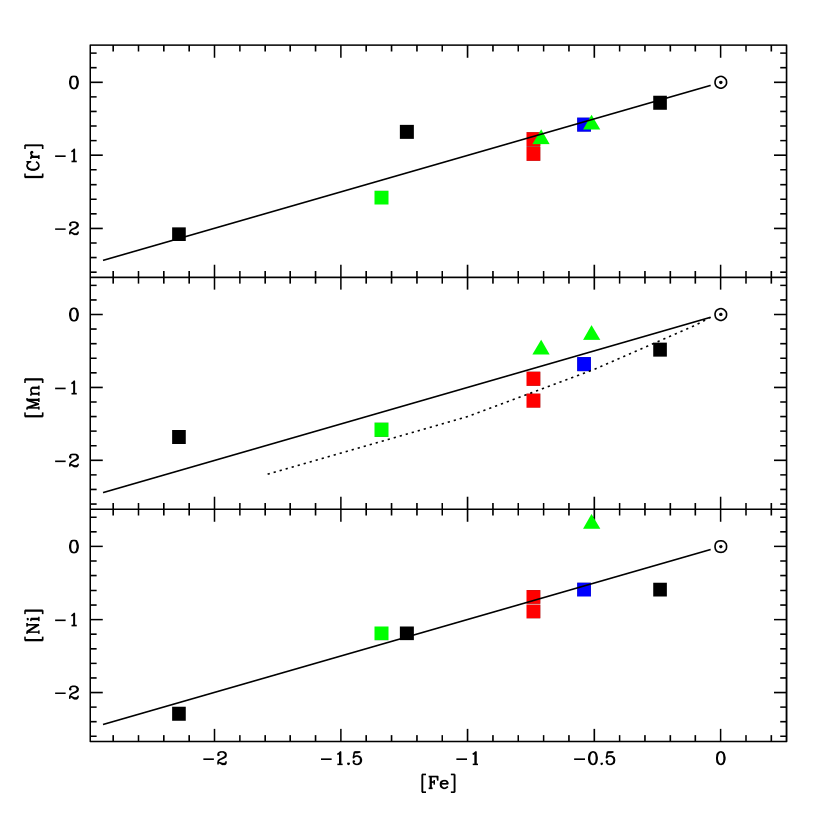
Figure 10: [Cr], [Mn], and [Ni] vs [Fe]. Our sample of seven EHes is represented by filled squares. Two cool EHes analysed by Pandey et al. (2001) are represented by filled triangles. $\odot$ represents Sun. [X] = [Fe] are denoted by the solid lines where X represents Cr, Mn, and Ni. The dotted line for Mn is from the relation [Mn/Fe] versus [Fe/H] for normal disk and halo stars given by B.E. Reddy (private communication) and Reddy et al. (2003).

A second group of elements expected to be unaffected or only slightly so by nuclear reactions associated with H- and He-burning is the $\alpha$-elements Mg, Si, S, and Ca and also Ti. The variation of these abundances with the Fe abundance is shown in Figure 11 together with a mean (denoted by $\alpha$) computed from the abundances of Mg, Si, and S. It is known that in metal-poor normal and unevolved stars that the abundance ratio $\alpha$/Fe varies with Fe (Ryde & Lambert, 2004; Goswami & Prantzos, 2000). This variation is characterized by the dotted line in the figure. Examination of Figure 11 suggests that the abundances of the $\alpha$-elements and Ti follow the expected trend with the dramatic exception of DY Cen.

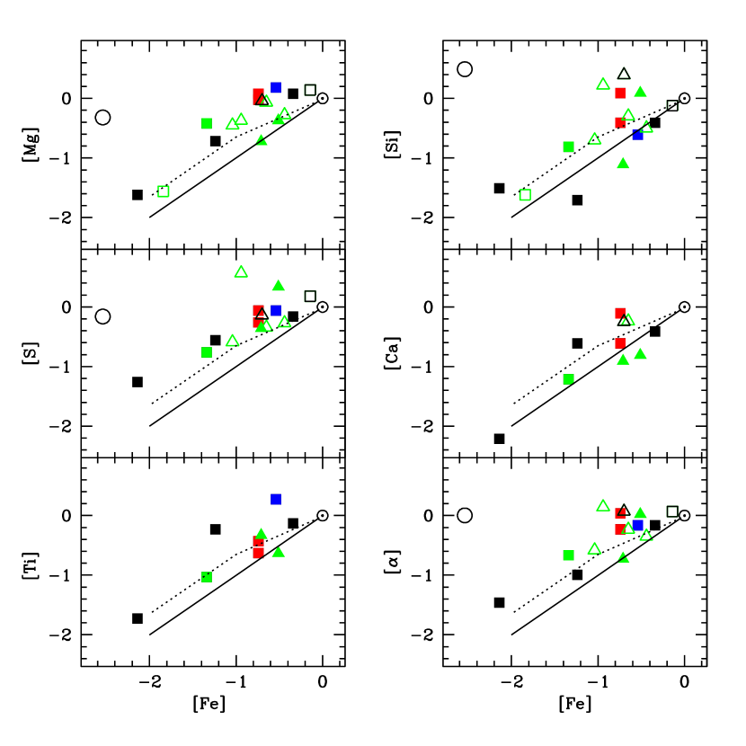
Figure 11: [Mg], [Si], [S], [Ca], [Ti], and [$\alpha$] vs [Fe]. Our sample of seven EHes is represented by filled squares. Two cool EHes analysed by Pandey et al. (2001) are represented by filled triangles. The results taken from the literature for the EHes with C/He of about 1% and much lower C/He are represented by open triangles and open squares, respectively. DY Cen is represented by open circle. $\odot$ represents Sun. [X] = [Fe] are denoted by the solid lines where X represents Mg, Si, S, Ca, Ti, and $\alpha$. The dotted lines are from the relation [X/Fe] versus [Fe/H] for normal disk and halo stars (Ryde & Lambert, 2004; Goswami & Prantzos, 2000).

Aluminum is another possible representative of initial metallicity. The Al abundances of the EHes follow the Fe abundances (Figure 12) with an apparent offset of about 0.4 dex in the Fe abundance. Again, DY Cen is a striking exception, but the other minority RCBs have an Al abundance in line with the general Al – Fe trend for the RCBs (Asplund et al., 2000). Note that, minority RCBs show lower Fe abundance and higher Si/Fe and S/Fe ratios than majority RCBs (Rao & Lambert, 1994). Pandey et al. (2001) found higher Si/Fe and S/Fe ratios for the Fe-poor cool EHe FQ Aqr than majority RCBs. But, from our adopted abundances (Table 4) for FQ Aqr, the Si/Fe and S/Fe ratios for FQ Aqr and majority RCBs are in concert.

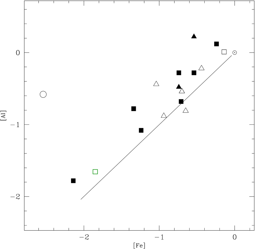
Figure 12: [Al] vs [Fe]. Our sample of seven EHes is represented by filled squares. Two cool EHes analysed by Pandey et al. (2001) are represented by filled triangles. The results taken from the literature for the EHes with C/He of about 1% and much lower C/He are represented by open triangles and open squares, respectively. DY Cen is represented by open circle. $\odot$ represents Sun. [Al] = [Fe] is denoted by the solid line.

In summary, several elements appear to be representative of initial metallicity. We take Fe for spectroscopic convenience as the representative of initial metallicity for the EHes but note the dramatic case of DY Cen. The representative of initial metallicity is used to predict the initial abundances of elements affected by nuclear reactions and mixing. Pandey et al. (2001) used Si and S as the representative of initial metallicity to derive the initial metallicity M$\equiv$Fe for the EHes. The initial metallicity M rederived from an EHe’s adopted Si and S abundances is consistent with its adopted Fe abundance.

5.2 Elements affected by evolution

Hydrogen – Deficiency of H shows a great range over the extended sample of EHes. The three least H-deficient stars are DY Cen, the hot RCB, and HD 144941 and V652 Her, the two EHes with a very low C abundance (see next section). The remaining EHe stars have H abundances $\log\epsilon$(H) in the range 5 to 8. There is a suggestion of a trend of increasing H with increasing $T_{\rm eff}$ but the hottest EHe LS IV$+6^{\circ}2$ does not fit the trend.

Carbon – The carbon abundances of our septet span a small but definite range: the mean C/He ratio is 0.0074 with a range from C/He = 0.0029 for FQ Aqr to 0.014 for V1920 Cyg. The mean C/He from eight of the ten additional EHes including DY Cen is 0.0058 with a range from 0.0029 to 0.0098. The grand mean from 15 stars is C/He = 0.0066. Two EHes – HD 144941 and V652 Her – have much lower C/He ratios: C/He $=1.8\times 10^{-5}$ and $4.0\times 10^{-5}$ for HD 144941 (Harrison & Jeffery, 1997) and V652 Her (Jeffery, Hill & Heber, 1999), respectively. This difference in the C/He ratios for EHes between the majority with C/He of about 0.7 per cent and HD 144941 and V652 Her suggests that a minimum of two mechanisms create EHes.

Nitrogen – Nitrogen is clearly enriched in the great majority of EHes above its initial abundance expected according to the Fe abundance. Figure 13 (left-hand panel) shows that the N abundance for all but 3 of the 17 stars follows the trend expected by the almost complete conversion of the initial C, N, and O to N through extensive running of the H-burning CN-cycle and the ON-cycles. The exceptions are again DY Cen (very N-rich for its Fe abundance) and HD 144941, one of two stars with a very low C/He ratio, and LSS 99, both with a N abundance indicating little N enrichment over the star’s initial N abundance.

Oxygen – Oxygen abundances relative to Fe range from underabundant by more than 1 dex to overabundant by almost 2 dex. The stars fall into two groups. Six stars with [O] $\geq 0$ stand apart from the remainder of the sample for which the majority (9 of 11) have an O abundance close to their initial value (Figure 13 (right-hand panel)). The O/N ratio for this majority is approximately constant at O/N $\simeq 1$ and independent of Fe. The O-rich stars in order of decreasing Fe abundance are: LSS 4357, LSE 78, V1920 Cyg, LS IV $-1^{\circ}2$, FQ Aqr, and DY Cen. The very O-poor star (relative to Fe) is V652 Her, one of two stars with a very low C/He. The other such star, HD 144941, has an O (and possibly N) abundance equal to its initial value.

A problem is presented by the stars with their O abundances close to the inferred initial abundances. Eight of the 10 have an N abundance indicating total conversion of initial C, N, and O to N via the CNO-cycles, yet the observed O abundance is close to the initial abundance (unlikely to be just a coincidence but the possibility needs to be explored).

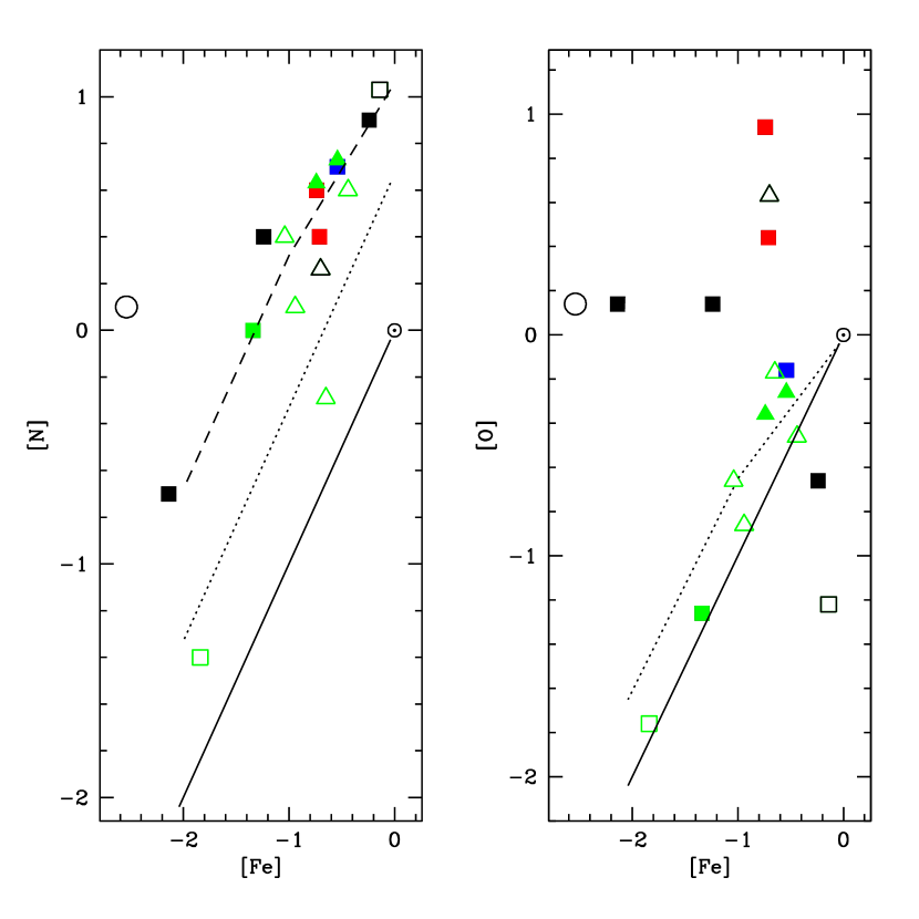
Figure 13: Left-hand panel, [N] vs [Fe]. Our sample of seven EHes is represented by filled squares. Two cool EHes analysed by Pandey et al. (2001) are represented by filled triangles. The results taken from the literature for the EHes with C/He of about 1% and much lower C/He are represented by open triangles and open squares, respectively. DY Cen is represented by open circle. $\odot$ represents Sun. [N] = [Fe] is denoted by the solid line. The dotted line represents conversion of the initial sum of C and N to N. The dashed line represents the locus of the sum of initial C, N, and O converted to N. Right-hand panel, [O] vs [Fe]. The symbols have the same meaning as in left-hand panel. [O] = [Fe] is denoted by the solid line. The dotted line is from the relation [O/Fe] versus [Fe/H] for normal disk and halo stars (Nissen et al., 2002).

Heavy elements – Yttrium and Zr abundances were measured from our STIS spectra. In addition, Y and Zr were measured in the cool EHe LS IV $-14^{\circ}109$ (Pandey et al., 2001). Yttrium and Zr abundances are shown in Figure 14 where we assume that [Zr] = [Fe] represents the initial abundances. Two stars are severely enriched in Y and Zr: V1920 Cyg and LSE 78 with overabundances of about a factor of 50 (1.7 dex) (see Figure 1 of Pandey et al. 2004). Also see Figure 15: the Zr iii line strength relative to the Fe ii line strength is enhanced in Zr enriched stars: LSE 78 and PV Tel, than the other two stars: FQ Aqr and BD+10^∘ 2179 with Zr close to their initial abundance. This obvious difference in line strengths is also seen in Figures 1 and 2. A third star PV Tel is enriched by a factor of about 10 (1.0 dex). The other five stars are considered to have their initial abundances of Y and Zr. We attribute the occurrence of Y and Zr overabundances to contamination of the atmosphere by $s$-process products.

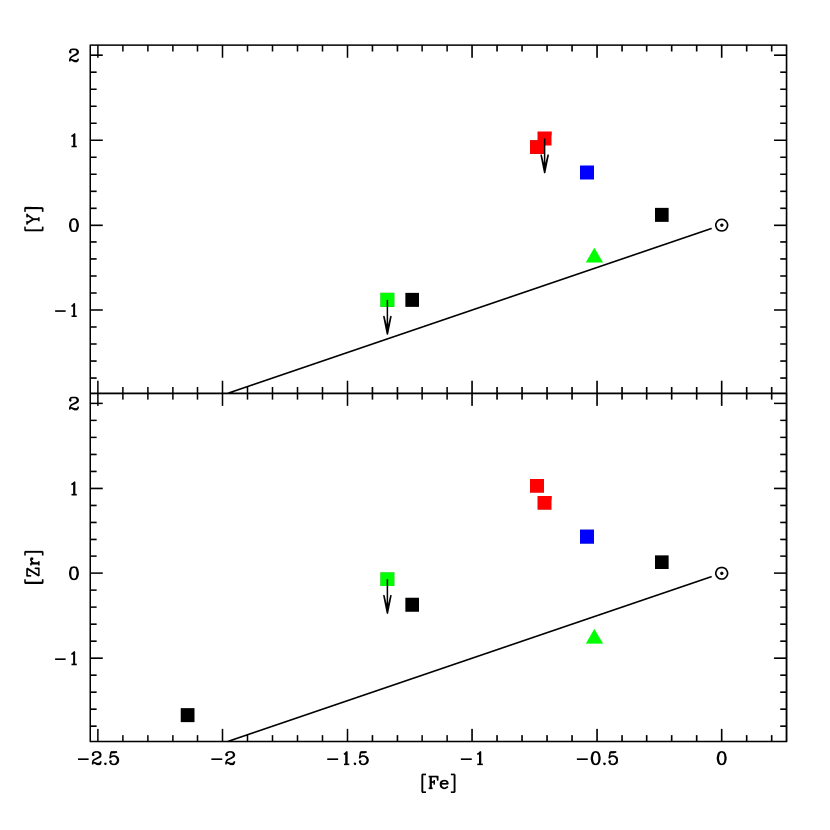
Figure 14: [Y] and [Zr] vs [Fe]. Our sample of seven EHes is represented by filled squares. One of the cool EHes LS IV $-14^{\circ}109$ analysed by Pandey et al. (2001) is represented by filled triangle. $\odot$ represents Sun. [X] = [Fe] are denoted by the solid lines where X represents Y and Zr.

Figure 15: The observed spectra of FQ Aqr, PV Tel, BD+10^∘ 2179, and LSE 78 are represented by filled circles. The left-hand panels show the region including the Zr iii line at 2086.78Å for FQ, Aqr and PV Tel. The right-hand panels show the region including the Zr iii line at 2620.57Å for BD+10^∘ 2179 and LSE 78. Synthetic spectra for three different Zr abundances are shown in each panel for these stars – see keys on the figure. In each panel, the principal lines are identified.

The STIS spectra provide only upper limits for rare-earths La, Ce, and Nd. In the case of V1920 Cyg, the Ce and Nd upper limits suggest an overabundance less than that of Y and Zr, again assuming that the initial abundances scale directly with the Fe abundance. For LSE 78, the La and Ce limits are consistent with the Y and Zr overabundances. A similar consistency is found for the Ce abundance in PV Tel. The cool EHe LS IV $-14^{\circ}109$ has a Ba abundance consistent with its initial abundances of Sr, Y, Zr, and Ba.

5.3 The R Coronae Borealis stars

Unlike the EHes where He and C abundances are determined spectroscopically, the He abundance of the RCBs, except for the rare hot RCBs, is not measurable. In addition, Asplund et al. (2000) identified that the observed strength of a C i line in RCB’s spectrum is considerably lower than the predicted and dubbed this ‘the carbon problem’. These factors introduce an uncertainty into the absolute abundances but Asplund et al. argue that the abundance ratios, say O/Fe, should be little affected.

The compositions of the RCBs (Asplund et al., 2000) show some similarities to those of the EHes but with differences. One difference is that the RCB and EHe metallicity distribution functions are offset by about 0.5 dex in Fe: the most Fe-rich RCBs have an Fe abundance about 0.5 dex less than their EHe counterparts. These offsets differ from element to element: e.g., the Ni distributions are very similar but the Ca distributions are offset similarly to Fe. These odd differences may be reflections of the inability to understand and resolve the carbon problem.

Despite these differences, there are similarities that support the reasonable view that the EHe and RCB stars are closely related. For example, RCBs’ O abundances fall into the two groups identified from a set of O-rich stars and a larger group with O close to the initial abundance. Also, a few RCBs are $s$-process enriched. Minority RCBs resemble DY Cen, which might be regarded first as RCB rather than an EHe. It is worthy of note that a few RCBs are known to be rich in lithium, which must be of recent manufacture. Lithium is not spectroscopically detectable in the EHes. In this context the search of light elements (Be and B) in the $STIS$ spectra of EHes was unsuccessful. B iii lines at 2065.776Å, and at 2067.233Å are not detected in EHes’ $STIS$ spectra. However, B iii line at 2065.776Å gives an upper limit to the Boron abundance of about 0.6 dex for BD $+10^{\circ}$ 2179. B iii line at 2067.233Å is severely blended by Fe iii line.

6 Merger of a He and a CO white dwarf

The expected composition of a EHe star resulting from the accretion of a helium white dwarf by a carbon-oxygen white dwarf was discussed by Saio & Jeffery (2002). This scenario is a leading explanation for EHes and RCBs for reasons of chemical composition and other fits to observations (Asplund et al., 2000; Pandey et al., 2001; Saio & Jeffery, 2002). Here, we examine afresh the evidence from the EHes’ compositions supporting the merger hypothesis.

In what follows, we consider the initial conditions and the mixing recipe adopted by Saio & Jeffery (2002; see also Pandey et al. 2001). The atmosphere and envelope of the resultant EHe is composed of two zones from the accreted He white dwarf, and three zones from the CO white dwarf which is largely undisturbed by the merger. Thermal flashes occur during the accretion phase but the attendant nucleosynthesis is ignored. We compare the recipe’s ability to account for the observed abundances of H, He, C, N, and O and their run with Fe. Also, we comment on the $s$-process enrichments.

The He white dwarf contributes its thin surface layer with a composition assumed to be the original mix of elements: this layer is denoted by the label He:H, as in $\beta$(H)_He:H which is the mass fraction of hydrogen in the layer of mass $m$(He:H) (in $M_{\odot}$). More importantly, the He white dwarf also contributes its He-rich interior (denoted by the label He:He). Saio & Jeffery took the composition of He:He to be CNO-processed, i.e., $\beta$(H) = 0, $\beta$(He) $\approx$ 1, $\beta$(C) = $\beta$(O) = 0, with $\beta$(N) equal to the sum of the initial mass fractions of C, N, and O, and all other elements at their initial mass fractions.

The CO white dwarf that accretes its companion contributes three parts to the five part mix. First, a surface layer (denoted by CO:H) with the original mix of elements. Second, the former He-shell (denoted by CO:He) with a composition either put identical to that of the He:He layer or enriched in C and O at the expense of He (see below for remarks on the layer’s $s$-process enrichment). To conclude the list of ingredients, material from the core may be added (denoted by CO:CO) with a composition dominated by C and O.

In the representative examples chosen by Saio & Jeffery (their Table 3), a 0.3$M_{\odot}$ He white dwarf is accreted by a 0.6$M_{\odot}$ CO white dwarf with the accreted material undergoing little mixing with the accretor. The dominant contributor by mass to the final mix for the envelope is the He:He layer with a mass of 0.3$M_{\odot}$ followed by the CO:He layer with a mass of about 0.03$M_{\odot}$ and the CO:CO layer with a mass of 0.007$M_{\odot}$ or less. Finally, the surface layers He:H and CO:H with a contribution each of 0.00002$M_{\odot}$ provide the final mix with a H deficiency of about 10^-4.

The stars – HD 144941 and V652 Her – with the very low C/He ratio are plausibly identified as resulting from the merger of a He white dwarf with a more massive He white dwarf (Saio & Jeffery, 2000) and are not further discussed in detail.

Hydrogen – Surviving hydrogen is contributed by the layers He:H and CO:H. The formal expression for the mass fraction of H, Z(H), in the EHe atmosphere is ${\rm Z(H)}=(\beta{\rm(H)}m_{\rm He:H}+\beta{\rm(H)}m_{\rm CO:H})/M_{tot}$ where $M_{tot}$ is the total mass of the five contributing layers, and $\beta$(H)_He:H and $\beta$(H)_CO:H are expected to be similar and equal to about 0.71. Thus, the residual H abundance of a EHe is – obviously – mainly set by the ratio of the combined mass of the two H-containing surface layers to the total mass of the final envelope and atmosphere. It is not difficult to imagine that these layers can be of low total mass and, hence, that a EHe may be very H-deficient.

Helium and Carbon – For the adopted parameters, primarily $M$(He:He)/$M$(CO:He) $\approx 10$ and $\beta$(He_He:He) $\simeq\beta$(He_CO:He) $\simeq 1$, the helium from the He:He layer effectively determines the final He abundance. The carbon (¹²C) is provided either by C from the top of the CO white dwarf (Saio & Jeffery’s recipe (1) in their Table 3) or from carbon in the CO:He layer as a result of He-burning (Saio & Jeffery’s recipe (2) in their Table 3). It is of interest to see if the fact that C/He ratio are generally similar across the EHe sample offers a clue to the source of the carbon.

In recipe (1), the C/He mass fraction is given approximately by the ratio
$M$(CO:CO)/$M$(He:He) assuming $\beta$(He)${}_{\rm He:He}\simeq\beta$(C)${}_{\rm CO:CO}\simeq 1$. Mass estimates of $M_{\rm CO:CO}\simeq 0.007$ and $M_{\rm He:He}\simeq 0.3$ (Saio & Jeffery 2002) give the number ratio C/He $\simeq 0.008$, a value close to the mean of the EHe sample.

In recipe (2) where the synthesised C is in the CO:He shell and the contribution by mass of the CO:CO layers is taken as negligible, the C/He mass fraction is approximately $\beta$(C)${}_{\rm CO:He}/\beta$(He)${}_{\rm He:He}\times M$(CO:He)/$M$(He:He). Again (of course), substitution from Saio & Jeffery’s Table 3 gives a number ratio for C/He that is at the mean observed value.

Nitrogen – The nitrogen (¹⁴N) is provided by the He:He and CO:He layers, principally the former on account of its ten times greater contribution to the total mass. Ignoring the CO:He layer, the N mass fraction is given by $Z$(N) = $\beta$(N)${}_{\rm He:He}M_{\rm He:He}/M_{tot}$ and the mass ratio N/He is given very simply as $Z$(N)/$Z$(He) = $\beta$(N)${}_{\rm He:He}/\beta$(He)_He:He. Not only is this ratio independent of the contributions of the various layers (within limits) but it is directly calculable from the initial abundances of C, N, and O which depend on the initial Fe abundance. This prediction which closely matches the observed N and He abundances at all Fe for all but three stars requires almost complete conversion of initial C, N, and O to N, as assumed for the layer He:He.

Oxygen – The oxygen (¹⁶O) is assumed to be a product of He-burning and to be contributed by either the CO:CO layer (recipe 1) or the CO:He layer (recipe 2). Since C and O are contributed by the same layer in both recipes, the O/C ratio is set by a simple ratio of mass fractions: $Z$(O)/$Z$(C) = $\beta$(O)${}_{\rm CO:CO}/\beta$(C)_CO:CO for recipe 1, and $\beta$(O)_CO:He/$\beta$(C)_CO:He for recipe 2. Saio & Jeffery adopt the ratio $\beta$(O)/$\beta$(C) = 0.25 for both layers from models of AGB stars, and, hence, one obtains the predicted O/C $=10^{-0.7}$, by number. This is probably insensitive to the initial metallicity of the AGB star.

The observed O/C across the sample of 15 EHes has a central value close to the prediction. Extreme values range from O/C = $10^{0.9}$ for V652 Her (most probably not the result of a He-CO merger), also possessing unusually low O, to $10^{-1.9}$ for BD $+10^{\circ}$ 2179. If these odd cases are dropped, the mean for the other 15 is O/C $=10^{-0.5}$, a value effectively the predicted one. The spread from $10^{+0.2}$ to $10^{-1.3}$ corresponding to a large range in the ratio of the O and C mass fractions from the contributing layer exceeds the assessed errors of measurement. The spread in O/C is dominated by that in O. For the group of six most oxygen rich EHes, the observed O/C ratios imply a ratio of the $\beta$s of slightly less than unity. The O abundance for most of the other EHes appears to be a star’s initial abundance. Although one may design a ratio of the $\beta$s that is metallicity dependent to account for this result, it is then odd that the O abundances follow the initial O – Fe relation.

This oddity is removed if the observed O abundances are indeed the initial values. This, of course, implies that O is preserved in the He:He layer, but, in considering nitrogen, we noted that the observed N abundances followed the trend corresponding to conversion of initial C, N, and O to N in the He:He layer. Since the ON-cycles operate at a higher temperature than the CN-cycle, conversion of C to N but not O to N is possible at ‘low’ temperatures. Additionally at low temperatures and low metallicity, the $pp$-chain may convert all H to He before the slower running ON-cycles have reduced the O abundance to its equilibrium value. If this speculation is to fit the observations, we must suppose that the measured N abundances are overestimated by about 0.3 dex in order that the N abundances be close to the sum of the initial C and N abundances. It remains to be shown that the He:He layer of a He white dwarf can be created by H-burning by the $pp$-chains and the CN-cycle and without operation of the ON-cycle.

Were the entire He:He layer exposed to the temperatures for ON-cycling, the reservoir of ³He needed to account for Li in some RCBs would be destroyed. The ³He is a product of main sequence evolution where the $pp$-chain partially operates well outside the H-burning core. This ³He is then later converted to ⁷Li by the Cameron-Fowler (1971) mechanism: ³He(⁴He,$\gamma)^{7}$Be$(e^{-},\nu)^{7}$Li. The level of the Li abundance, when present, is such that large-scale preservation of ³He seems necessary prior to the onset of the Cameron-Fowler mechanism. This is an indirect indication that the He:He layer was not in every case heated such that the CNO-cycles converted all C,N, and O to N. (Lithium production through spallation reactions on the stellar surface is not an appealing alternative. One unattractive of spallation is that it results in a ratio ⁷Li/⁶Li $\sim 1$ but observations suggest that the observed lithium is almost pure ⁷Li.)

Yttrium and Zirconium – The $s$-process enrichment is sited in the CO:He and CO:CO layers. Saio & Jeffery assumed an enrichment by a factor of 10 in the CO:He. This factor and the small mass ratio $M$(CO:He)$/M_{tot}$ result in very little enrichment for the EHe. Observed Y and Zr enrichments require either a greater enrichment in the CO:He layer or addition of material from the CO:CO layer. Significantly, the two most obviously $s$-process enriched EHes are also among the most O-rich.

7 Concluding remarks

This LTE model atmosphere analysis of high-resolution STIS spectra undertaken primarily to investigate the abundances of $s$-process elements in the EHe stars has shown that indeed a few EHes exhibit marked overabundances of Y and Zr. The STIS spectra additionally provide abundances of other elements and, in particular, of several Fe-group elements not observable in optical spectra. We combine the results of the STIS analysis with abundance analyses based on newly obtained or published optical spectra. Our results for seven EHes and approximately 24 elements per star are supplemented with abundances taken from the literature for an additional ten EHes. The combined sample of 17 stars with abundances obtained in a nearly uniform manner provides the most complete dataset yet obtained for these very H-deficient stars.

Our interpretation of the EHe’s atmospheric compositions considers simple recipes based on the idea that the EHe is a consequence of the accretion of a He white dwarf by a more massive CO white dwarf. (Two stars of low C/He ratio are more probably a result of the merger of two He white dwarfs.) These recipes adapted from Saio & Jeffery (2002) are quite successful. A EHe’s initial composition is inferred from the measured Fe abundance, but other elements from Al to Ni could equally well be identified as the representative of initial metallicity. Saio & Jeffery’s recipes plausibly account for the H, He, C, and N abundances and for the O abundance of a few stars. Other stars show an O abundance similar to the expected initial abundance. This similarity would seem to require that the He-rich material of the He white dwarf was exposed to the CN-cycle but not the ON-cycles.

Further progress in elucidating the origins of the EHes from determinations of their chemical compositions requires two principal developments. First, the abundance analyses should be based on Non-LTE atmospheres and Non-LTE line formation. The tools to implement these two steps are available but limitations in available atomic data may need to be addressed. In parallel with this work, a continued effort should be made to include additional elements. Neon is of particular interest as ²²Ne is produced from ¹⁴N by $\alpha$-captures prior to the onset of He-burning by the $3\alpha$-process. Hints of Ne enrichment exist (Pandey et al., 2001). Second, a rigorous theoretical treatment of the merger of the He white dwarf with the CO white dwarf must be developed with inclusion of the hydrodynamics and the nucleosynthesis occurring during and following the short-lived accretion process. A solid beginning has been made in this direction, see, for example Guerrero, García-Berro & Isern (2004).

There remains the puzzling case of DY Cen and the minority RCBs (Rao & Lambert, 1994) with their highly anomalous composition. Are these anomalies the result of very peculiar set of nuclear processes? Or has the ‘normal’ composition of a RCB been altered by fractionation in the atmosphere or circumstellar shell?

Appendix A Appendix material: Lines used for abundance analysis

The lines used for the abundance analysis of LSE 78, BD +10^∘ 2179, V1920 Cyg, HD 124448, PV Tel, LS IV-1^∘ 2, and FQ Aqr are given in the Tables 11 to 20 (available only in electronic edition). The $gf$-value, the lower excitation potential ($\chi$), log of Stark damping constant/electron number density ($\Gamma_{el}$), log of radiative damping constant ($\Gamma_{rad}$), and the abundance (log $\epsilon$) derived for each line are listed. Also listed are the equivalent widths ($W_{\lambda}$) corresponding to the abundances derived by spectrum synthesis for most individual lines. The symbol ? follows uncertain abundances, and ‘Synth’ in the sixth column implies spectrum synthesis.

References

Artru = Artru et al. (1981)
CL = Crespo Lopez-Urrutia et al. (1994)
Ekberg = Ekberg (1997)
Jeffery = Jeffery, Woolf, & Pollacco (2001)
Kurucz = Kurucz’s database
Luck = Compilations by R. E. Luck
NIST = NIST database
Pandey = Pandey et al. (2004)
RU = Raassen & Uylings (1997)
Salih = Salih, Lawler, & Whaling (1985)
UR = Uylings & Raassen (1997)
WFD = Wiese, Fuhr, & Deters (1996)

Table 11: Ultraviolet lines used to derive elemental abundances for LSE 78 with the model atmosphere (18300, 2.2, 16.0)

Ion
$\lambda$(Å)	log $gf$	$\chi$(eV)	$\Gamma_{el}$	$\Gamma_{rad}$	$W_{\lambda}$(mÅ)	log $\epsilon$	Ref a
He i
2652.566	–1.410	3.267			Synth	11.54	Kurucz
C ii
1988.530	–2.123	16.333			108	9.4	WFD
2092.165	–1.473	20.704			58	9.6	WFD
2173.849	–1.185	14.449	–4.930	9.050	Synth	9.3?	WFD
2174.168	–1.486	14.449	–4.930	9.050	Synth	9.3?	WFD
2269.688	–0.810	22.537			86	9.8	WFD
2401.759	–1.353	16.332		8.770	Synth	9.3	WFD
2402.399	–1.052	16.333		8.770	Synth	9.1	WFD
2426.620	–2.913	18.046			Synth	9.3	WFD
2426.650	–2.214	18.046			Synth	9.3	WFD
2426.710	–1.959	18.046			Synth	9.3	WFD
2509.124	–0.767	13.716		9.680	466	9.6	WFD
2511.734	–1.466	13.721		9.680	Synth	9.5	WFD
2512.054	–0.512	13.721		9.680	Synth	9.5	WFD
2554.478	–1.000	21.734			22	9.0	WFD
2574.770	–0.620	18.046			Synth	9.2	WFD
2574.865	–0.470	18.046			Synth	9.2	WFD
2574.865	–1.770	18.046			Synth	9.2	WFD
2620.208	–1.507	18.655			73	9.2?	WFD
2622.535	–2.653	18.656			Synth	9.5	WFD
2622.887	–1.699	18.656			Synth	9.5	WFD
2640.533	–0.689	22.528		8.080	Synth	9.7	WFD
2640.583	–0.483	22.529		8.080	Synth	9.7	WFD
2640.893	–0.299	22.533		8.080	Synth	9.7	WFD
2641.393	–0.136	22.537		8.080	Synth	9.7	WFD
2641.534	–1.086	22.529		8.080	Synth	9.7	WFD
2642.333	–0.972	22.533		8.080	45	9.5	WFD
2643.282	–2.231	22.532		8.080	Synth	9.6	WFD
2643.433	–1.079	22.537		8.080	Synth	9.6	WFD
2669.833	–2.663	18.046			Synth	9.3	WFD
2669.866	–1.964	18.046			Synth	9.3	WFD
2669.935	–1.709	18.046			Synth	9.3	WFD
Mean:							9.39$\pm$0.25$\pm$0.06
C iii
1908.730	–6.729	0.000		2.640	338	9.4?	WFD
2162.926	0.604	34.280		10.020	86	9.75	WFD
2296.871	–0.264	12.690		9.240	Synth	9.6?	WFD
Mean:							9.57$\pm$0.15$\pm$0.29
N ii
2142.775	–6.359	0.016			Synth	8.0?	WFD
2206.087	–1.591	20.409		8.150	Synth	$<$8.7	WFD
2316.488	–1.006	20.654	–4.740	8.140	Synth	$<$8.2	WFD
2316.678	–1.177	20.646	–4.740	8.860	Synth	$<$8.2	WFD
2317.038	–0.846	20.666	–4.740	8.120	Synth	$<$8.2	WFD
Mg ii
2449.561	–0.790	8.864			Synth	7.6	Kurucz
2449.561	–2.090	8.864			Synth	7.6	Kurucz
2449.613	–0.950	8.864			Synth	7.6	Kurucz
2660.754	–0.480	8.864	–3.510		Synth	7.8	NIST
2660.756	–1.780	8.864	–3.510		Synth	7.8	NIST
2660.818	–0.630	8.864	–3.510		Synth	7.8	NIST
Mean:							7.70$\pm$0.14$\pm$0.15
Al ii
1990.533	0.640	7.421			115	6.0	NIST
Mean:							6.00$\pm$0.00$\pm$0.24
Al iii
1935.840	0.730	14.377			Synth	6.0	NIST
1935.863	–0.570	14.377			Synth	6.0	NIST
1935.949	0.570	14.377			Synth	6.0	NIST
Mean:							6.00$\pm$0.00$\pm$0.07
Si ii
2072.015	–0.432	6.858		8.400	Synth	7.2	NIST
2072.695	–1.572	6.859		8.400	Synth	7.1	NIST
2072.700	–0.272	6.859		8.410	Synth	7.1	NIST
Mean:							7.15$\pm$0.07$\pm$0.11
Si iii
2541.818	–0.809	10.276		9.420	387	6.9	NIST
2559.196	0.730	20.552		9.750	104	6.5	NIST
Mean:							6.70$\pm$0.28$\pm$0.19
Ti iii
2199.216	0.090	10.390	–6.356	9.251	10	4.4	NIST
2334.340	–0.540	4.736	–6.699	8.916	84	4.4	NIST
2346.783	0.132	4.764	–6.700	8.916	138	4.1	NIST
2413.987	0.373	5.171	–6.673	9.033	139	4.0	NIST
2540.048	0.204	4.719	–6.642	8.962	166	4.2	RU
2565.408	–0.128	4.736	–6.652	8.838	176	4.6	RU
2567.556	–0.137	4.719	–6.630	9.013	159	4.5	NIST
2580.443	–0.526	4.764	–6.653	8.838	83	4.4	RU
Mean:							4.33$\pm$0.21$\pm$0.09
Cr iii
2013.818	–0.233	8.187	–6.746	9.097	Synth	4.7	Ekberg
2013.869	–0.785	8.652	–6.793	9.161	Synth	4.7	Ekberg
2117.551	0.522	6.250	–6.787	8.924	Synth	4.7	Ekberg
2117.905	–0.450	6.136	–6.752	9.190	Synth	4.7	Ekberg
2139.133	0.492	7.863	–6.798	8.736	132	4.7	Ekberg
2141.189	0.483	6.250	–6.756	9.134	175	4.5	Ekberg
2147.217	0.036	6.178	–6.749	9.004	86	4.3	Ekberg
2149.518	0.119	8.170	–6.742	9.053	60	4.6	Ekberg
2152.773	0.125	8.187	–6.743	9.076	Synth	4.9	Ekberg
2152.806	–0.129	8.722	–6.749	9.076	Synth	4.9	Ekberg
2154.649	–0.349	7.833	–6.750	8.760	30	4.6	Ekberg
2159.110	–0.208	7.863	–6.796	8.734	Synth	4.7	Ekberg
2159.749	–0.371	8.739	–6.722	9.111	Synth	4.6	Ekberg
2166.272	0.199	8.211	–6.744	9.076	56	4.5	Ekberg
2182.685	–0.321	8.801	–6.778	9.076	Synth	4.8	Ekberg
2182.787	–0.279	7.833	–6.741	8.736	Synth	4.8	Ekberg
2190.770	0.486	8.211	–6.754	9.134	102	4.6	Ekberg
2197.908	0.231	8.170	–6.749	9.134	Synth	4.7	Ekberg
2198.635	0.580	8.887	–6.787	8.719	Synth	4.9	Ekberg
2203.229	0.262	7.863	–6.746	9.176	113	4.8	Ekberg
2204.574	–0.327	8.187	–6.749	9.134	38	4.8	Ekberg
2217.516	0.666	9.342	–6.777	9.013	69	4.5	Ekberg
2219.584	–0.052	7.863	–6.743	9.170	43	4.5	Ekberg
2226.678	0.654	6.250	–6.765	8.631	200	4.5	Ekberg
2231.802	0.143	7.024	–6.753	8.960	104	4.6	Ekberg
2233.791	0.280	7.066	–6.753	8.962	121	4.6	Ekberg
2237.584	0.452	7.120	–6.753	8.965	144	4.6	Ekberg
2244.117	0.387	6.178	–6.762	8.620	193	4.7	Ekberg
2247.691	0.475	10.461	–6.755	9.009	21	4.4	Ekberg
2251.473	0.248	6.153	–6.760	8.616	174	4.7	Ekberg
2258.632	0.459	9.342	–6.738	9.316	68	4.7	Ekberg
2262.650	0.150	10.486	–6.751	9.009	44	5.1	Ekberg
2264.924	–0.408	6.153	–6.759	8.613	93	4.8	Ekberg
2273.360	0.573	8.911	–6.748	9.097	84	4.6	Ekberg
2275.475	0.484	8.894	–6.746	9.097	Synth	4.8	Ekberg
2276.428	0.445	8.187	–6.741	8.687	Synth	4.9	Ekberg
2277.483	0.404	8.887	–6.745	9.093	Synth	4.8	Ekberg
2284.481	0.457	8.637	–6.746	8.767	105	4.8	Ekberg
2289.258	0.224	8.637	–6.706	8.892	65	4.7	Ekberg
2290.675	0.370	8.170	–6.740	8.675	100	4.7	Ekberg
2310.040	–0.218	8.843	–6.736	9.009	Synth	4.7	Ekberg
2310.044	–0.605	8.843	–6.735	9.009	Synth	4.7	Ekberg
2314.627	0.341	7.024	–6.722	8.975	103	4.4	Ekberg
2456.813	–0.727	7.066	–6.682	8.905	26	4.7	Ekberg
2479.818	–0.060	7.066	–6.691	8.922	86	4.7	Ekberg
2483.072	0.191	7.120	–6.682	8.905	90	4.5	Ekberg
2531.023	–0.412	7.024	–6.718	8.934	40	4.6	Ekberg
2544.373	–0.610	7.120	–6.726	9.076	26	4.6	Ekberg
2587.417	–0.160	8.911	–6.743	8.677	21	4.6	Ekberg
2616.517	–0.317	8.894	–6.741	8.687	14	4.5	Ekberg
Mean:							4.66$\pm$0.15$\pm$0.10
Mn iii
1947.516	–0.285	7.780	–6.820	8.814	Synth	$<$4.1	UR
2069.044	0.554	7.846	–6.802	8.696	143	4.1	UR
2169.773	0.529	10.582	–6.756	8.822	60	4.3	UR
2176.882	0.435	10.564	–6.755	8.810	83	4.6	UR
2215.233	0.095	8.873	–6.739	9.021	91	4.5	UR
2227.451	0.412	8.950	–6.739	9.021	129	4.5	UR
2409.301	–0.269	8.950	–6.743	8.859	32	4.3	UR
Mean:							4.38$\pm$0.18$\pm$0.11
Fe ii
2348.115	–0.472	0.232	–6.788	8.615	Synth	6.7	NIST
2348.303	–0.210	0.083	–6.585	8.486	Synth	6.7	NIST
2379.276	–0.992	0.301	–6.788	8.615	56	6.9	NIST
2380.762	–0.692	0.083	–6.588	8.484	105	6.9	NIST
2384.387	–1.105	0.387	–6.788	8.614	52	7.0	NIST
2388.630	–0.180	0.048	–6.601	8.535	159	6.7	NIST
2395.626	0.333	0.048	–6.599	8.539	226	6.6	NIST
2399.242	–0.139	0.083	–6.602	8.533	130	6.5	NIST
2404.887	0.072	0.083	–6.601	8.535	199	6.7	NIST
2406.662	–0.255	0.107	–6.602	8.531	143	6.7	NIST
2410.520	–0.105	0.107	–6.602	8.533	Synth	6.5	NIST
2411.069	–0.377	0.121	–6.603	8.531	Synth	6.8	NIST
2413.311	–0.415	0.121	–6.602	8.531	116	6.7	NIST
2428.365	0.380	3.903	–6.577	8.540	95	7.0	NIST
2432.874	0.600	4.076	–6.583	8.610	90	6.8	NIST
2439.302	0.540	3.153	–6.586	8.528	95	6.6	NIST
2460.440	0.760	5.484	–5.824	8.957	Synth	6.7	NIST
2461.284	0.270	3.230	–6.589	8.515	Synth	6.9	NIST
2461.862	0.374	3.221	–6.585	8.521	Synth	6.9	NIST
2503.875	0.360	3.768	–6.566	8.740	84	6.9	NIST
2533.628	0.180	2.657	–6.634	8.473	Synth	6.9	NIST
2534.419	–0.050	2.692	–6.657	8.479	Synth	7.0	NIST
2535.362	0.105	5.571	–6.629	8.728	Synth	7.1	NIST
2535.486	–0.380	2.807	–6.644	8.509	Synth	7.1	NIST
2562.536	–0.050	0.986	–6.593	8.528	179	7.0	NIST
2566.913	–0.650	1.076	–6.588	8.530	79	7.0	NIST
2570.849	0.010	3.814	–6.646	8.699	53	7.0	NIST
2587.945	0.148	4.154	–6.607	8.583	46	6.9	NIST
2591.543	–0.510	1.040	–6.593	8.528	86	6.9	NIST
2592.785	0.530	4.076	–6.627	8.465	108	7.0	NIST
2598.370	–0.102	0.048	–6.687	8.462	155	6.6	NIST
2607.088	–0.159	0.083	–6.688	8.462	156	6.6	NIST
2611.874	–0.045	0.048	–6.686	8.464	160	6.5	NIST
2613.825	–0.387	0.107	–6.688	8.462	132	6.7	NIST
2619.075	–0.556	2.807	–6.665	8.612	37	7.0	NIST
2621.670	–0.995	0.121	–6.688	8.462	82	7.0	NIST
2625.668	–0.452	0.048	–6.685	8.468	141	6.8	NIST
2628.294	–0.448	0.121	–6.688	8.462	138	6.8	NIST
2666.637	0.170	3.425	–6.608	8.528	95	7.0	NIST
Mean:							6.82$\pm$0.17$\pm$0.22
Fe iii
1986.259	–1.391	8.256	–6.857	9.146	189	7.0	Kurucz
2029.524	–0.283	11.211	–6.820	9.179	186	6.8	Kurucz
2050.743	–0.279	8.641	–6.848	9.250	293	6.8	Kurucz
2053.524	–0.710	9.541	–6.818	9.013	Synth	6.8	Kurucz
2054.492	–0.350	11.579	–6.863	9.241	Synth	7.0	Kurucz
2059.687	0.240	9.560	–6.818	9.013	306	6.7	Kurucz
2070.539	0.363	10.344	–6.796	8.999	290	6.7	Kurucz
2083.534	0.007	11.132	–6.828	8.980	213	6.7	Kurucz
2087.909	–0.240	9.556	–6.798	9.004	Synth	7.1	Kurucz
2088.623	–0.920	8.765	–6.821	8.900	Synth	6.8	Kurucz
2089.093	–0.670	9.560	–6.798	9.004	Synth	6.9	Kurucz
2092.951	–0.014	11.211	–6.814	9.064	246	7.0	Kurucz
2112.501	–1.037	11.472	–6.853	8.852	93	6.9	Kurucz
2116.593	–0.729	8.659	–6.852	8.984	246	6.9	Kurucz
2118.564	–0.861	8.653	–6.855	9.093	228	6.9	Kurucz
2134.806	–2.610	8.765	–6.818	8.794	Synth	6.8	Kurucz
2135.520	–1.010	11.025	–6.872	8.926	Synth	6.8	Kurucz
2151.780	0.058	10.899	–6.806	8.791	227	6.7	Kurucz
2156.189	–1.169	10.899	–6.834	9.143	96	6.9	Kurucz
2157.711	–0.743	9.156	–6.787	8.961	195	6.7	Kurucz
2166.958	–0.723	9.156	–6.788	8.995	238	7.0	Kurucz
2178.673	–1.540	10.993	–6.859	8.882	Synth	7.0	Kurucz
2179.260	–1.761	9.541	–6.857	9.072	Synth	7.2	Kurucz
2180.412	–0.549	9.156	–6.789	9.004	248	6.9	Kurucz
2221.829	–1.321	9.141	–6.821	9.243	104	6.6	Kurucz
2238.152	–0.409	11.579	–6.828	9.140	150	6.8	Kurucz
2243.411	–1.558	8.769	–6.842	8.757	113	6.8	Kurucz
2267.445	–0.945	11.472	–6.852	9.097	99	6.9	Kurucz
2306.579	–1.994	9.141	–6.821	8.984	51	6.8	Kurucz
2349.792	–1.994	10.218	–6.821	9.004	34	6.9	Kurucz
2353.818	–1.258	10.214	–6.830	9.093	93	6.8	Kurucz
2389.530	–0.481	11.472	–6.806	8.791	127	6.7	Kurucz
2415.107	–1.607	9.541	–6.790	9.009	75	6.8	Kurucz
2421.509	–1.585	10.435	–6.845	9.021	70	7.0	Kurucz
2501.514	–1.798	10.214	–6.863	8.981	46	6.9	Kurucz
2608.103	–1.240	10.308	–6.868	8.849	87	6.7	Kurucz
2609.686	–2.100	10.311	–6.868	8.849	35	7.0	Kurucz
2662.337	–1.895	10.461	–6.875	9.228	64	7.2	Kurucz
Mean:							6.87$\pm$0.14$\pm$0.13
Co iii
1942.366	–0.302	5.914	–6.857	8.739	Synth	4.4	Kurucz
1942.506	0.012	9.086	–6.859	9.114	Synth	4.4	Kurucz
1977.031	0.000	6.990	–6.858	9.212	94	4.4	Kurucz
Mean:							4.40$\pm$0.00$\pm$0.13
Ni ii
2165.550	0.230	1.041	–6.639	8.574	127	5.5	NIST
2169.092	–0.050	1.157	–6.640	8.593	93	5.6	NIST
2206.712	–0.013	1.254	–6.640	8.593	109	5.7	NIST
2216.477	0.480	1.041	–6.639	8.594	136	5.3	NIST
2222.950	–0.140	1.041	–6.649	8.547	72	5.5	NIST
2253.848	–0.043	1.322	–6.651	8.576	101	5.7	NIST
2264.461	–0.056	1.254	–6.652	8.568	119	5.8	NIST
2270.212	0.081	1.157	–6.649	8.547	146	5.8	NIST
2278.770	0.120	1.680	–6.630	8.817	80	5.5	NIST
2341.208	0.173	3.604	–6.612	8.635	41	5.7	Kurucz
2394.523	0.165	1.680	–6.633	8.545	86	5.5	NIST
2416.135	0.170	1.859	–6.628	8.521	79	5.5	NIST
2510.874	–0.260	1.680	–6.649	8.547	58	5.7	NIST
Mean:							5.60$\pm$0.15$\pm$0.20
Ni iii
2405.930	–1.127	8.851	–6.929	8.817	50	5.5	Kurucz
2448.360	–0.971	8.811	–6.930	8.815	64	5.5	Kurucz
Mean:							5.50$\pm$0.00$\pm$0.17
Zn ii
2025.483	–0.086	0.000	–6.670		Synth	$<$4.4	NIST
Mean:							$<$4.40$\pm$0.00$\pm$0.21
Y iii
2414.643	–0.385	0.000			Synth	$<$3.2	Pandey
Mean:							$<$3.20$\pm$0.00$\pm$0.20
Zr iii
2664.269	0.380	3.108			Synth	3.7	Pandey
2643.806	0.290	2.422			Synth	3.5	Pandey
2620.570	0.560	2.422			Synth	3.4	Pandey
2006.810	–0.160	0.712			Synth	3.4	Pandey
Mean:							3.50$\pm$0.14$\pm$0.17
Ce iii
2603.591	0.310	2.003			Synth	$<$2.6	Pandey
Mean:							$<$2.60$\pm$0.00$\pm$0.15

Table 12: Ultraviolet lines used to derive elemental abundances for BD +10^∘ 2179 with the model atmosphere (16900, 2.55, 4.5)

Ion
$\lambda$(Å)	log $gf$	$\chi$(eV)	$\Gamma_{el}$	$\Gamma_{rad}$	$W_{\lambda}$(mÅ)	log $\epsilon$	Ref a
C ii
1916.010	–2.369	14.449			59	8.9	WFD
1926.770	–2.366	13.716			Synth	9.5	WFD
1927.020	–2.065	13.716			Synth	9.5	WFD
1988.530	–2.123	16.333			78	9.6	WFD
2017.929	–1.793	16.332		8.600	Synth	9.4	WFD
2018.379	–1.492	16.333		8.600	Synth	9.3?	WFD
2092.165	–1.473	20.704			39	9.6	WFD
2137.416	–0.991	16.332			Synth	9.4	WFD
2137.896	–0.735	16.333			Synth	9.4	WFD
2137.926	–1.690	16.333			Synth	9.4	WFD
2156.262	–1.107	22.899			29	9.7	WFD
2173.849	–1.185	14.449	–4.930	9.050	Synth	9.4	WFD
2174.168	–1.486	14.449	–4.930	9.050	Synth	9.4	WFD
2187.476	–1.712	20.920			Synth	9.6	WFD
2188.375	–1.014	20.922			Synth	9.6	WFD
2242.114	–1.222	23.119			21	9.7	WFD
2323.137	–2.876	18.046			Synth	9.3	WFD
2323.497	–8.305	0.000		1.286	Synth	9.3	WFD
2324.686	–6.927	0.000		2.233	Synth	9.4	WFD
2325.396	–6.592	0.008		1.741	Synth	9.3	WFD
2326.926	–7.439	0.008		1.286	57	9.2	WFD
2328.125	–6.906	0.008		2.233	96	9.4	WFD
2401.759	–1.353	16.332		8.770	Synth	9.2	WFD
2402.399	–1.052	16.333		8.770	Synth	9.1	WFD
2426.620	–2.913	18.046			Synth	9.4	WFD
2426.650	–2.214	18.046			Synth	9.4	WFD
2426.710	–1.959	18.046			Synth	9.4	WFD
2430.770	–1.624	22.899			15	9.9	WFD
2509.124	–0.767	13.716		9.680	292	9.6	WFD
2604.872	–1.034	22.537			32	9.6	WFD
2620.208	–1.507	18.655			42	9.1	WFD
2622.535	–2.653	18.656			Synth	9.6	WFD
2622.887	–1.699	18.656			Synth	9.2	WFD
2640.533	–0.689	22.528		8.080	Synth	9.4	WFD
2640.583	–0.483	22.529		8.080	Synth	9.4	WFD
2640.893	–0.299	22.533		8.080	Synth	9.4	WFD
2641.393	–0.136	22.537		8.080	Synth	9.3	WFD
2641.534	–1.086	22.529		8.080	Synth	9.3	WFD
2642.333	–0.972	22.533		8.080	Synth	9.4	WFD
2643.282	–2.231	22.532		8.080	Synth	9.4	WFD
2643.433	–1.079	22.537		8.080	Synth	9.4	WFD
2669.833	–2.663	18.046			Synth	9.4	WFD
2669.866	–1.964	18.046			Synth	9.4	WFD
2669.935	–1.709	18.046			Synth	9.4	WFD
Mean:							9.43$\pm$0.21$\pm$0.09
C iii
1908.730	–6.729	0.000		2.640	129	9.4	WFD
2010.090	–0.156	32.202			22	9.6	WFD
Mean:							9.50$\pm$0.14$\pm$0.37
N ii
2142.775	–6.359	0.016			Synth	7.7?	WFD
2206.087	–1.591	20.409		8.150	Synth	8.64?	WFD
Mg ii
2449.561	–0.790	8.864			Synth	7.1	Kurucz
2449.561	–2.090	8.864			Synth	7.1	Kurucz
2449.613	–0.950	8.864			Synth	7.1	Kurucz
2660.754	–0.480	8.864	–3.510		Synth	7.3	NIST
2660.756	–1.780	8.864	–3.510		Synth	7.3	NIST
2660.818	–0.630	8.864	–3.510		Synth	7.3	NIST
Mean:							7.20$\pm$0.11$\pm$0.11
Al ii
1855.926	–0.890	4.636	–5.360		55	5.9	NIST
1990.533	0.640	7.421			76	5.7	NIST
Mean:							5.80$\pm$0.14$\pm$0.21
Al iii
1935.840	0.730	14.377			Synth	6.0	NIST
1935.863	–0.570	14.377			Synth	6.0	NIST
1935.949	0.570	14.377			Synth	6.0	NIST
Mean:							6.00$\pm$0.00$\pm$0.17
Si ii
1902.451	0.000	9.839			54	7.2	Kurucz
2059.015	–1.000	6.858			28	6.7	Kurucz
2072.015	–0.432	6.858		8.400	Synth	7.4	NIST
2072.695	–1.572	6.859		8.400	Synth	7.2	NIST
2072.700	–0.272	6.859		8.410	Synth	7.2	NIST
2308.746	–0.830	9.839			11	7.0	Kurucz
2500.945	–0.670	9.837	–3.850	9.410	12	6.9	NIST
2501.988	–0.510	9.839	–3.850	9.410	11	6.7	NIST
Mean:							7.01$\pm$0.27$\pm$0.14
Si iii
2541.818	–0.809	10.276		9.420	159	6.9	NIST
2546.092	–0.520	20.552		9.830	20	7.2	NIST
2559.196	0.730	20.552		9.750	33	6.4	NIST
Mean:							6.83$\pm$0.40$\pm$0.22
Ti iii
1935.306	0.069	9.599	–6.295	9.320	Synth	4.0?	Kurucz
2346.783	0.132	4.764	–6.700	8.916	46	3.7	NIST
2413.987	0.373	5.171	–6.673	9.033	59	3.9	NIST
2516.066	0.471	4.764	–6.672	8.765	67	3.9	NIST
2527.845	0.360	4.736	–6.647	8.943	59	3.8	RU
2540.048	0.204	4.719	–6.642	8.962	48	3.7	RU
2565.408	–0.128	4.736	–6.652	8.838	46	4.0	RU
2567.556	–0.137	4.719	–6.630	9.013	33	3.7	NIST
2576.463	–0.561	4.736	–6.630	9.013	27	4.0	NIST
2580.443	–0.526	4.764	–6.653	8.838	28	4.0	RU
Mean:							3.86$\pm$0.13$\pm$0.11
Cr iii
2047.264	0.495	8.911	–6.800	9.176	20	4.1	Ekberg
2100.492	–0.442	6.211	–6.705	8.905	10	3.8	Ekberg
2103.337	–0.301	6.211	–6.787	8.924	18	4.0	Ekberg
2106.820	–0.445	6.153	–6.725	8.912	12	3.9	Ekberg
2114.894	0.392	6.211	–6.780	9.004	60	4.3	Ekberg
2117.551	0.522	6.250	–6.787	8.924	Synth	4.0	Ekberg
2117.905	–0.450	6.136	–6.752	9.190	Synth	4.0	Ekberg
2131.983	–0.201	8.211	–6.749	9.064	7	4.0	Ekberg
2139.133	0.492	7.863	–6.798	8.736	24	3.9	Ekberg
2141.189	0.483	6.250	–6.756	9.134	32	3.6	Ekberg
2147.217	0.036	6.178	–6.749	9.004	35	4.1	Ekberg
2149.518	0.119	8.170	–6.742	9.053	25	4.4	Ekberg
2152.773	0.125	8.187	–6.743	9.076	Synth	4.4	Ekberg
2152.806	–0.129	8.722	–6.749	9.076	Synth	4.4	Ekberg
2157.205	0.064	8.703	–6.787	9.111	12	4.2	Ekberg
2159.110	–0.208	7.863	–6.796	8.734	Synth	4.4	Ekberg
2159.749	–0.371	8.739	–6.722	9.111	Synth	4.4	Ekberg
2166.272	0.199	8.211	–6.744	9.076	20	4.2	Ekberg
2182.685	–0.321	8.801	–6.778	9.076	Synth	4.2	Ekberg
2182.787	–0.279	7.833	–6.741	8.736	Synth	4.2	Ekberg
2197.908	0.231	8.170	–6.749	9.134	Synth	4.0	Ekberg
2198.635	0.580	8.887	–6.787	8.719	Synth	3.9	Ekberg
2203.229	0.262	7.863	–6.746	9.176	22	4.1	Ekberg
2204.574	–0.327	8.187	–6.749	9.134	8	4.2	Ekberg
2207.443	–0.798	7.833	–6.743	9.170	5	4.4	Ekberg
2217.516	0.666	9.342	–6.777	9.013	20	4.1	Ekberg
2218.697	0.293	9.273	–6.763	9.204	Synth	4.1	Ekberg
2219.584	–0.052	7.863	–6.743	9.170	Synth	4.1	Ekberg
2226.678	0.654	6.250	–6.765	8.631	56	4.0	Ekberg
2231.802	0.143	7.024	–6.753	8.960	32	4.2	Ekberg
2233.791	0.280	7.066	–6.753	8.962	28	4.0	Ekberg
2237.584	0.452	7.120	–6.753	8.965	31	3.9	Ekberg
2244.117	0.387	6.178	–6.762	8.620	45	4.0	Ekberg
2257.396	–0.246	6.211	–6.762	8.620	Synth	4.1	Kurucz
2257.547	0.575	8.211	–6.744	8.677	Synth	4.1	Ekberg
2264.924	–0.408	6.153	–6.759	8.613	21	4.2	Ekberg
2284.481	0.457	8.637	–6.746	8.767	20	4.1	Ekberg
2286.591	–0.369	8.211	–6.742	8.687	7	4.2	Ekberg
2289.258	0.224	8.637	–6.706	8.892	11	4.0	Ekberg
2290.675	0.370	8.170	–6.740	8.675	22	4.1	Ekberg
2300.510	0.339	8.637	–6.737	9.064	9	3.8	Ekberg
2314.627	0.341	7.024	–6.722	8.975	39	4.2	Ekberg
2479.818	–0.060	7.066	–6.691	8.922	21	4.2	Ekberg
2483.072	0.191	7.120	–6.682	8.905	22	4.0	Ekberg
2544.373	–0.610	7.120	–6.726	9.076	11	4.4	Ekberg
2616.517	–0.317	8.894	–6.741	8.687	5	4.2	Ekberg
Mean:							4.11$\pm$0.18$\pm$0.12
Mn ii
2119.773	–0.227	4.823	–6.722	8.702	Synth	3.9?	Kurucz
2576.105	0.433	0.000	–6.602	8.481	Synth	4.0	Kurucz
2576.175	0.284	6.493	–6.545	8.507	Synth	4.0	Kurucz
2593.724	0.270	0.000	–6.605	8.471	11	3.9	NIST
2605.684	0.140	0.000	–6.607	8.465	12	4.0	NIST
Mean:							3.95$\pm$0.06$\pm$0.21
Mn iii
1942.892	0.259	11.073	–6.826	8.933	17	4.3	UR
1947.516	–0.285	7.780	–6.820	8.814	13	3.7	UR
1956.624	–0.316	7.758	–6.784	8.859	29	4.2	UR
2026.928	–0.523	7.744	–6.784	9.233	Synth	4.0	UR
2027.106	–0.802	7.758	–6.783	9.233	Synth	4.0	UR
2027.803	0.500	11.073	–6.819	8.869	Synth	3.8	UR
2027.872	0.317	8.950	–6.807	9.072	Synth	3.8	UR
2028.093	0.153	10.734	–6.793	9.140	Synth	3.8	UR
2028.156	0.352	10.744	–6.793	9.146	Synth	4.0	UR
2028.231	0.075	11.041	–6.776	9.199	Synth	4.0	UR
2031.515	–0.310	7.758	–6.784	9.233	22	4.0	UR
2048.949	0.686	10.582	–6.812	8.705	22	3.9	UR
2066.372	0.542	10.548	–6.806	8.703	21	4.0	UR
2069.044	0.554	7.846	–6.802	8.696	56	4.0	UR
2077.369	0.368	7.810	–6.800	8.689	44	3.9	UR
2121.405	–0.011	10.560	–6.769	8.843	8	4.0	UR
2126.144	0.521	12.056	–6.775	9.104	15	4.3	UR
2130.592	0.183	10.669	–6.766	8.876	6	3.7	UR
2169.773	0.529	10.582	–6.756	8.822	26	4.2	UR
2176.882	0.435	10.564	–6.755	8.810	14	3.9	UR
2181.851	0.337	10.548	–6.753	8.806	14	4.0	UR
2211.952	0.264	11.742	–6.787	8.902	Synth	3.8	UR
2212.439	–0.111	8.852	–6.739	9.021	Synth	3.8	UR
2215.233	0.095	8.873	–6.739	9.021	22	4.0	UR
2227.451	0.412	8.950	–6.739	9.021	25	3.8	UR
2250.063	–0.117	11.073	–6.769	8.816	8	4.3	UR
2266.585	–0.280	11.400	–6.732	8.938	5	4.4	UR
2374.314	–0.231	8.950	–6.761	8.839	16	4.2	UR
2409.301	–0.269	8.950	–6.743	8.859	9	3.9	UR
Mean:							4.00$\pm$0.19$\pm$0.14
Fe ii
2249.180	–1.604	0.000	–6.666	8.615	13	6.2	NIST
2253.127	–1.470	0.048	–6.603	8.491	19	6.3	NIST
2279.916	–1.517	0.048	–6.601	8.476	21	6.4	NIST
2327.397	–0.672	0.083	–6.583	8.489	44	6.1	NIST
2332.800	–0.140	0.048	–6.585	8.486	72	6.2	NIST
2338.008	–0.432	0.107	–6.583	8.489	55	6.1	NIST
2348.115	–0.366	0.232	–6.788	8.615	Synth	6.1	NIST
2348.303	–0.210	0.083	–6.585	8.486	Synth	6.1	NIST
2364.829	–0.388	0.048	–6.588	8.484	58	6.1	NIST
2368.596	–0.690	0.352	–6.788	8.614	39	6.1	NIST
2369.955	0.760	5.222	–5.827	8.994	39	6.3	NIST
2373.736	–0.554	0.000	–6.599	8.539	56	6.2	NIST
2379.276	–0.992	0.301	–6.788	8.615	35	6.3	NIST
2382.039	0.589	0.000	–6.596	8.548	94	6.2	NIST
2384.387	–1.105	0.387	–6.788	8.614	29	6.3	NIST
2388.630	–0.180	0.048	–6.601	8.535	66	6.1	NIST
2391.478	–1.635	0.301	–6.788	8.476	14	6.4	NIST
2395.626	0.333	0.048	–6.599	8.539	83	6.1	NIST
2399.242	–0.139	0.083	–6.602	8.533	63	6.0	NIST
2404.432	–0.910	0.107	–6.603	8.531	Synth	6.1	NIST
2404.887	0.072	0.083	–6.601	8.535	Synth	6.3	NIST
2406.662	–0.255	0.107	–6.602	8.531	62	6.1	NIST
2410.520	–0.105	0.107	–6.602	8.533	Synth	6.1	NIST
2411.069	–0.377	0.121	–6.603	8.531	Synth	6.1	NIST
2413.311	–0.415	0.121	–6.602	8.531	55	6.1	NIST
2428.365	0.380	3.903	–6.577	8.540	46	6.4	NIST
2432.874	0.600	4.076	–6.583	8.610	44	6.2	NIST
2439.302	0.540	3.153	–6.586	8.528	47	6.0	NIST
2458.784	0.468	3.199	–6.576	8.533	52	6.2	NIST
2460.440	0.760	5.484	–5.824	8.957	Synth	6.2	NIST
2461.284	0.270	3.230	–6.589	8.515	Synth	6.2	NIST
2461.862	0.374	3.221	–6.585	8.521	Synth	6.1	NIST
2469.516	0.187	3.903	–6.577	8.744	24	6.1	NIST
2475.543	0.410	5.589	–5.821	8.956	23	6.4	NIST
2493.262	0.710	2.635	–6.613	8.508	69	6.2	NIST
2503.875	0.360	3.768	–6.566	8.740	33	6.1	NIST
2533.628	0.180	2.657	–6.634	8.473	Synth	6.5	NIST
2534.419	–0.050	2.692	–6.657	8.479	Synth	6.5	NIST
2535.362	0.105	5.571	–6.629	8.728	Synth	6.4	NIST
2535.486	–0.380	2.807	–6.644	8.509	Synth	6.4	NIST
2546.671	–0.320	2.828	–6.644	8.509	35	6.5	NIST
2550.684	0.020	3.245	–6.616	8.574	39	6.4	NIST
2562.536	–0.050	0.986	–6.593	8.528	61	6.2	NIST
2566.913	–0.650	1.076	–6.588	8.530	38	6.3	NIST
2570.849	0.010	3.814	–6.646	8.699	26	6.3	NIST
2577.923	–0.600	1.097	–6.588	8.530	26	6.0	NIST
2582.584	–0.470	1.076	–6.590	8.529	41	6.2	NIST
2585.876	–0.187	0.000	–6.686	8.464	74	6.4	NIST
2587.945	0.148	4.154	–6.607	8.583	27	6.3	NIST
2591.543	–0.510	1.040	–6.593	8.528	44	6.3	NIST
2599.396	0.348	0.000	–6.685	8.468	90	6.4	NIST
2607.088	–0.159	0.083	–6.688	8.462	59	5.8	NIST
2611.074	–1.430	1.076	–6.593	8.528	Synth	6.3	NIST
2611.874	–0.045	0.048	–6.686	8.464	Synth	6.1	NIST
2613.825	–0.387	0.107	–6.688	8.462	66	6.2	NIST
2617.618	–0.566	0.083	–6.687	8.462	49	6.0	NIST
2619.075	–0.556	2.807	–6.665	8.612	29	6.5	NIST
2621.670	–0.995	0.121	–6.688	8.462	42	6.3	NIST
2625.668	–0.452	0.048	–6.685	8.468	76	6.5	NIST
2628.294	–0.448	0.121	–6.688	8.462	75	6.5	NIST
2666.637	0.170	3.425	–6.608	8.528	43	6.3	NIST
Mean:							6.23$\pm$0.16$\pm$0.19
Fe iii
1852.679	0.256	11.147	–6.883	9.290	Synth	6.0	Kurucz
1852.817	–0.559	10.320	–6.859	9.079	Synth	6.0	Kurucz
1856.685	–0.134	8.659	–6.870	8.989	66	5.7	Kurucz
1859.811	0.222	11.579	–6.829	8.927	Synth	6.0	Kurucz
1859.954	–0.477	8.653	–6.873	9.041	Synth	6.0	Kurucz
1869.821	–0.110	7.872	–6.857	9.093	Synth	6.1	Kurucz
1869.841	–0.666	7.872	–6.857	9.093	Synth	6.1	Kurucz
1870.582	–1.671	8.248	–6.816	8.995	Synth	6.1	Kurucz
1871.152	–0.121	7.872	–6.858	9.146	Synth	5.9	Kurucz
1873.539	–0.703	10.320	–6.874	9.097	37	6.1	Kurucz
1893.984	0.420	9.901	–6.852	9.230	91	6.2	Kurucz
1895.456	0.461	3.731	–6.881	8.775	247	6.5	Kurucz
1896.814	0.480	9.900	–6.850	9.230	97	6.3	Kurucz
1898.869	–0.220	9.141	–6.867	9.344	77	6.2	Kurucz
1903.259	–0.530	9.156	–6.867	9.344	59	6.1	Kurucz
1907.576	0.570	9.899	–6.854	9.250	93	6.1	Kurucz
1912.917	–0.620	8.256	–6.855	9.241	55	5.8	Kurucz
1914.056	0.344	3.731	–6.877	8.763	193	6.3	Kurucz
1916.510	–0.098	10.308	–6.885	8.818	49	5.8	Kurucz
1920.187	–0.156	10.311	–6.883	8.770	70	6.4	Kurucz
1925.265	–0.441	10.498	–6.868	9.097	61	6.5	Kurucz
1931.505	0.510	8.641	–6.871	8.849	101	6.1	Kurucz
1932.817	–0.185	10.335	–6.884	8.927	65	6.3	Kurucz
1937.349	0.410	7.872	–6.875	8.751	112	6.3	Kurucz
1938.895	0.435	10.435	–6.873	8.926	80	6.1	Kurucz
1950.334	0.670	11.025	–6.878	8.840	74	5.9	Kurucz
1953.318	0.435	9.899	–6.864	8.903	Synth	6.3	Kurucz
1953.326	0.310	8.769	–6.852	9.228	Synth	6.3	Kurucz
1957.936	0.414	11.594	–6.862	9.053	58	5.9	Kurucz
1960.318	0.727	9.899	–6.873	8.736	106	6.4	Kurucz
1964.170	0.355	9.900	–6.859	8.924	73	5.8	Kurucz
1965.311	0.158	10.498	–6.862	8.989	Synth	5.9	Kurucz
1966.068	0.115	12.233	–6.836	9.223	Synth	6.1	Kurucz
1966.740	0.413	10.993	–6.868	8.852	Synth	6.1	Kurucz
1976.131	–0.094	8.241	–6.853	8.984	95	6.3	Kurucz
1982.078	–0.723	8.248	–6.856	9.093	76	6.4	Kurucz
1986.259	–1.391	8.256	–6.857	9.146	27	5.9	Kurucz
1994.075	0.280	7.871	–6.842	8.719	103	6.1	Kurucz
2005.083	–0.549	8.248	–6.839	8.772	74	6.2	Kurucz
2006.266	–0.732	8.256	–6.841	8.897	67	6.2	Kurucz
2008.469	–0.565	8.256	–6.838	8.702	74	6.2	Kurucz
2017.288	0.040	11.147	–6.853	9.149	60	6.2	Kurucz
2026.043	0.338	11.025	–6.836	8.984	81	6.4	Kurucz
2038.092	–0.369	9.156	–6.858	9.033	49	5.7	Kurucz
2039.510	0.550	11.472	–6.848	9.064	64	5.9	Kurucz
2042.239	–0.450	10.228	–6.826	8.768	39	5.9	Kurucz
2050.743	–0.279	8.641	–6.848	9.250	84	6.3	Kurucz
2053.524	–0.710	9.541	–6.818	9.013	54	6.3	Kurucz
2059.687	0.240	9.560	–6.818	9.013	84	6.1	Kurucz
2067.309	0.104	11.147	–6.835	8.984	54	6.0	Kurucz
2070.539	0.363	10.344	–6.796	8.999	82	6.2	Kurucz
2078.992	0.316	5.083	–6.817	9.061	184	6.4	Kurucz
2087.138	0.150	9.541	–6.806	9.093	Synth	6.1	Kurucz
2087.909	–0.240	9.556	–6.798	9.004	Synth	6.3	Kurucz
2088.623	–0.920	8.765	–6.821	8.900	Synth	6.6	Kurucz
2089.093	–0.670	9.560	–6.798	9.004	Synth	6.6	Kurucz
2103.809	0.130	8.769	–6.791	9.009	95	6.3	Kurucz
2107.322	0.100	8.769	–6.791	8.996	84	6.0	Kurucz
2108.679	–0.655	10.498	–6.837	8.799	35	6.1	Kurucz
2116.593	–0.729	8.659	–6.852	8.984	73	6.5	Kurucz
2118.564	–0.861	8.653	–6.855	9.093	42	5.9	Kurucz
2134.806	–2.610	8.765	–6.818	8.794	Synth	6.1	Kurucz
2144.743	–0.694	10.344	–6.844	8.780	35	6.1	Kurucz
2151.780	0.058	10.899	–6.806	8.791	54	6.0	Kurucz
2157.711	–0.743	9.156	–6.787	8.961	53	6.2	Kurucz
2166.958	–0.723	9.156	–6.788	8.995	49	6.1	Kurucz
2171.046	–0.649	9.167	–6.787	8.995	56	6.2	Kurucz
2221.829	–1.321	9.141	–6.821	9.243	32	6.3	Kurucz
2243.411	–1.558	8.769	–6.842	8.757	31	6.4	Kurucz
2595.622	–1.228	9.899	–6.845	8.898	19	6.2	Kurucz
2617.147	–0.828	11.594	–6.793	8.999	14	6.0	Kurucz
Mean:							6.15$\pm$0.21$\pm$0.15
Ni ii
2128.578	–0.870	1.254	–6.617	8.653	11	4.9	MFW
2165.550	0.230	1.041	–6.639	8.574	59	4.9	NIST
2169.092	–0.050	1.157	–6.640	8.593	49	5.0	NIST
2175.142	–0.123	1.254	–6.644	8.590	49	5.1	NIST
2179.352	–0.301	3.079	–6.610	8.606	39	5.7	Kurucz
2184.602	–0.081	1.322	–6.649	8.587	Synth	5.0	NIST
2185.503	0.234	3.104	–6.620	8.610	Synth	5.1	Kurucz
2201.405	–0.250	1.322	–6.644	8.590	42	5.1	NIST
2205.548	0.870	6.633	–5.889	9.048	18	5.2	Kurucz
2206.712	–0.013	1.254	–6.640	8.593	54	5.1	NIST
2213.195	–0.442	2.950	–6.642	8.576	15	5.2	Kurucz
2216.477	0.480	1.041	–6.639	8.594	83	5.2	NIST
2222.950	–0.140	1.041	–6.649	8.547	56	5.2	NIST
2224.864	–0.036	1.157	–6.652	8.568	54	5.1	NIST
2226.328	–0.240	1.254	–6.651	8.576	43	5.1	NIST
2253.848	–0.043	1.322	–6.651	8.576	56	5.2	NIST
2264.461	–0.056	1.254	–6.652	8.568	47	5.0	NIST
2270.212	0.081	1.157	–6.649	8.547	67	5.3	NIST
2274.725	–0.500	3.073	–6.637	8.754	15	5.3	Kurucz
2278.317	0.207	4.032	–6.639	8.903	Synth	5.1	Kurucz
2278.770	0.120	1.680	–6.630	8.817	Synth	4.9	NIST
2287.081	–0.060	1.859	–6.637	8.844	Synth	5.1	MFW
2287.645	0.028	3.104	–6.637	8.754	Synth	5.1	Kurucz
2298.267	0.120	1.859	–6.616	8.741	46	5.0	NIST
2299.653	–0.172	2.865	–6.653	8.574	15	4.9	Kurucz
2302.992	0.140	1.157	–6.667	8.531	66	5.2	NIST
2312.917	0.527	4.029	–6.622	8.544	30	5.0	Kurucz
2316.036	0.268	1.041	–6.721	8.522	64	5.0	NIST
2318.508	–0.538	3.104	–6.384	8.749	11	5.2	Kurucz
2319.751	–0.403	3.104	–6.619	8.624	15	5.2	Kurucz
2326.451	–0.970	1.322	–6.466	8.533	16	5.2	NIST
2341.208	0.173	3.604	–6.612	8.635	25	5.1	Kurucz
2394.523	0.165	1.680	–6.633	8.545	54	5.1	NIST
2416.135	0.170	1.859	–6.628	8.521	56	5.2	NIST
2510.874	–0.260	1.680	–6.649	8.547	39	5.2	NIST
Mean:							5.12$\pm$0.15$\pm$0.19
Ni iii
1890.131	–0.811	9.826	–6.918	8.952	13	5.0	Kurucz
2405.930	–1.127	8.851	–6.929	8.817	7	4.8	Kurucz
2448.360	–0.971	8.811	–6.930	8.815	15	5.1	Kurucz
2524.350	–1.376	9.813	–6.936	9.326	6	5.3	Kurucz
Mean:							5.05$\pm$0.21$\pm$0.19
Zn ii
2025.483	–0.086	0.000	–6.670		Synth	4.4	NIST
Mean:							4.40$\pm$0.00$\pm$0.19
Y iii
2414.643	–0.385	0.000			Synth	$<$1.6	Pandey
2367.227	–0.107	0.090			Synth	$<$1.4	Pandey
Mean:							$<$1.40$\pm$0.00$\pm$0.18
Zr iii
2620.570	0.560	2.422			Synth	2.2	Pandey
2420.672	–0.370	2.281			Synth	$<$2.5	Pandey
2086.780	0.040	0.712			Synth	$<$2.2	Pandey
2006.810	–0.160	0.712			Synth	2.6	Pandey
1863.972	–0.500	0.000			Synth	$<$2.6	Pandey
Mean:							$<$2.60$\pm$0.00$\pm$0.17
Ce iii
2603.591	0.310	2.003			Synth	$<$2.0	Pandey
Mean:							$<$2.00$\pm$0.00$\pm$0.13

Table 13: Optical lines used to derive elemental abundances for BD +10^∘ 2179 with the model atmosphere (16400, 2.35, 6.5)

Ion
$\lambda$(Å)	log $gf$	$\chi$(eV)	$\Gamma_{el}$	$\Gamma_{rad}$	$W_{\lambda}$(mÅ)	log $\epsilon$	Ref a
H i
4101.734	–0.753	10.150		8.790	Synth	8.2	Jeffery
4340.462	–0.447	10.150		8.790	Synth	8.2	Jeffery
4861.323	–0.020	10.150		8.780	Synth	8.5	Jeffery
Mean:							8.30$\pm$0.17$\pm$0.20
He i
3819.600	–2.959	20.964			Synth	11.54	Jeffery
3819.600	–1.790	20.964			Synth	11.54	Jeffery
3819.600	–1.040	20.964			Synth	11.54	Jeffery
3819.610	–1.790	20.964			Synth	11.54	Jeffery
3819.610	–1.310	20.964			Synth	11.54	Jeffery
3819.760	–1.660	20.964			Synth	11.54	Jeffery
3867.470	–2.060	20.964			Synth	11.54	Jeffery
3867.480	–2.280	20.964			Synth	11.54	Jeffery
3867.630	–2.750	20.964			Synth	11.54	Jeffery
3871.790	–1.851	21.218			Synth	11.54	Jeffery
3926.540	–1.650	21.218			Synth	11.54	Jeffery
3935.910	–2.780	21.218			Synth	11.54	Jeffery
3964.730	–1.290	20.616	–2.571	7.982	Synth	11.54	Jeffery
4009.260	–1.470	21.218			Synth	11.54	Jeffery
4026.200	–0.370	20.964			Synth	11.54	Jeffery
4120.810	–1.529	20.957	–3.540	6.823	Synth	11.54	Jeffery
4120.990	–2.432	20.957	–3.540	6.823	Synth	11.54	Jeffery
4168.970	–2.340	21.218			Synth	11.54	Jeffery
4168.970	–2.319	21.211	–3.062	8.827	Synth	11.54	Jeffery
4437.550	–2.018	21.211	–3.463	8.826	Synth	11.54	Jeffery
4471.500	0.053	20.964			Synth	11.54	Jeffery
4713.140	–1.071	20.957	–4.007	7.015	Synth	11.54	Jeffery
4713.370	–1.975	20.957	–4.007	7.015	Synth	11.54	Jeffery
5015.680	–0.818	20.609	–4.109	8.351	Synth	11.54	Jeffery
5047.740	–1.588	21.211	–3.830	8.833	Synth	11.54	Jeffery
C i
4932.049	–1.658	7.685	–4.320		13	9.3	WFD
5052.167	–1.303	7.685	–4.510		28	9.3	WFD
Mean:							9.30$\pm$0.00$\pm$0.25
C ii
3918.980	–0.533	16.333	–5.042	8.788	286	9.4	WFD
3920.690	–0.232	16.334	–5.043	8.787	328	9.4	WFD
4017.272	–1.031	22.899			43	9.3	WFD
4021.166	–1.333	22.899			27	9.3	WFD
4306.330	–1.684	21.150	–4.692	8.484	46	9.5	WFD
4307.581	–1.383	20.150			77	9.3	WFD
4313.100	–0.373	23.120	–5.167	8.839	83	9.3	WFD
4317.260	–0.005	23.120	–5.168	8.838	113	9.3	WFD
4318.600	–0.407	23.120	–5.168	8.838	80	9.3	WFD
4321.650	–0.901	23.120	–5.169	8.837	45	9.3	WFD
4323.100	–1.105	23.120	–5.169	8.837	45	9.5	WFD
4325.830	–0.373	23.120	–5.170	8.837	Synth	9.4	WFD
4326.160	–0.407	23.120	–5.170	8.837	Synth	9.4	WFD
4637.630	–1.229	21.150	–4.757	8.420	75	9.5	WFD
4638.919	–0.973	20.150			Synth	9.2	WFD
4639.068	–1.928	20.150			Synth	9.4	WFD
4862.580	–1.479	19.495			63	9.1	WFD
4867.066	–1.781	19.495			35	9.0	WFD
5032.128	–0.143	20.922			174	9.5	WFD
5035.943	–0.399	20.920			113	9.1	WFD
5121.828	–1.199	20.150			Synth	9.2	WFD
5122.085	–0.530	20.845			Synth	9.2	WFD
5122.271	–0.359	20.845			Synth	9.2	WFD
5125.208	–1.597	20.150			51	9.3	WFD
5126.963	–1.899	20.150			32	9.3	WFD
5132.947	–0.211	20.701		8.950	Synth	9.8?	WFD
5133.281	–0.178	20.704		8.950	Synth	9.8?	WFD
5137.257	–0.911	20.701		8.950	91	9.3	WFD
5139.174	–0.707	20.704		8.950	118	9.4	WFD
5143.495	–0.212	20.704		8.950	166	9.4	WFD
5145.165	0.189	20.710		8.950	207	9.4	WFD
5151.085	–0.179	20.710		8.950	169	9.4	WFD
Mean:							9.32$\pm$0.12$\pm$0.04
C iii
4186.900	0.918	40.010	–4.956	9.378	19	9.8	WFD
4647.420	0.070	29.535	–5.382	9.349	51	9.3	WFD
4650.250	–0.151	29.535	–5.382	9.348	42	9.3	WFD
4651.470	–0.629	29.535	–5.383	9.348	27	9.3	WFD
Mean:							9.43$\pm$0.25$\pm$0.38
N ii
3842.180	–0.692	21.150	–5.011	9.239	30	8.0	WFD
3955.851	–0.813	18.466			68	8.0	WFD
3994.996	0.208	18.498	–5.434	9.350	139	7.8	WFD
4179.670	–0.204	23.250	–4.454	9.042	23	8.0	WFD
4227.740	–0.061	21.600	–5.056	8.531	42	7.8	WFD
4447.030	0.228	20.411	–5.544	9.166	75	7.7	WFD
4507.560	–0.817	20.666		9.330	25	8.0	WFD
4601.480	–0.428	18.468	–5.546	9.152	79	7.9	WFD
4607.160	–0.507	18.464	–5.547	9.151	73	7.9	WFD
4613.870	–0.665	18.468	–5.548	9.149	61	7.9	WFD
4643.090	–0.359	18.484	–5.553	9.144	88	7.9	WFD
4654.531	–1.404	18.497			20	7.8	WFD
4667.208	–1.533	18.497			20	8.0	WFD
4674.908	–1.463	18.497			19	7.9	WFD
4779.720	–0.587	20.650	–5.358	9.590	34	8.0	WFD
4781.190	–1.308	20.650	–5.358	9.590	9	7.9	WFD
4788.130	–0.363	20.650	–5.359	9.589	35	7.8	WFD
4810.310	–1.084	20.660	–5.363	9.585	17	8.1	WFD
4895.117	–1.338	17.877			18	7.6	WFD
4994.360	–0.164	25.500	–5.369	8.885	Synth	7.8	WFD
4994.370	–0.069	20.940	–5.430	9.340	Synth	7.8	WFD
5001.134	0.263	20.646	–5.470	8.450	Synth	7.9	WFD
5001.474	0.441	20.654	–5.470	8.430	Synth	7.9	WFD
5002.700	–1.022	18.480	–5.558	9.215	42	8.0	WFD
5005.150	0.594	20.666	–5.470	8.250	Synth	7.8	WFD
5005.300	–0.912	25.498		8.830	Synth	7.7	WFD
5007.328	0.171	20.940	–5.430	9.330	52	7.7	WFD
5010.620	–0.607	18.470	–5.559	9.214	71	8.0	WFD
5025.659	–0.547	20.666	–5.470	8.430	28	7.9	WFD
5045.090	–0.407	18.460	–5.565	9.208	87	8.0	WFD
Mean:							7.89$\pm$0.12$\pm$0.14
O ii
4072.157	0.552	25.643	–4.952	8.460	26	7.4	WFD
4185.449	0.604	28.351	–4.921	8.463	11	7.5	WFD
4189.789	0.717	28.354	–4.921	8.462	20	7.9	WFD
4336.860	–0.763	22.973	–5.237	9.008	11	7.5	WFD
4345.567	–0.346	22.979	–5.600	8.960	18	7.4	WFD
4349.426	0.060	22.993	–5.238	9.008	32	7.4	WFD
4366.888	–0.348	22.993	–5.237	9.007	15	7.3	WFD
4414.901	0.172	23.435	–5.202	9.604	33	7.5	WFD
4416.973	–0.077	23.413	–5.202	9.604	26	7.5	WFD
4641.817	0.055	22.973	–5.248	9.008	32	7.5	WFD
4649.143	0.308	22.993	–5.248	9.008	41	7.5	WFD
Mean:							7.49$\pm$0.15$\pm$0.23
Mg ii
4481.130	0.730	8.863	–4.600	8.823	Synth	7.00	NIST
4481.150	–0.570	8.864			Synth	7.00	NIST
4481.330	0.575	8.863	–4.600	8.823	Synth	7.00	NIST
5264.140	–0.138	11.569			25	7.20	NIST
Mean:							7.10$\pm$0.14$\pm$0.18
Al iii
4512.540	0.419	17.808	–5.075	8.743	41	5.6	NIST
4528.910	–0.280	17.818	–5.078	8.740	Synth	5.6	NIST
4529.200	0.671	17.740	–5.078	8.740	Synth	5.6	NIST
Mean:							5.60$\pm$0.00$\pm$0.10
Si ii
3853.660	–1.603	6.858	–5.064	8.042	44	6.9	NIST
3856.020	–0.652	6.860	–5.065	8.041	99	6.6	NIST
3862.600	–0.902	6.858	–5.066	8.040	72	6.5	NIST
4130.872	–0.841	9.839	–4.870	9.440	Synth	6.4	NIST
4130.890	0.464	9.839	–4.474	9.308	Synth	6.4	NIST
5041.030	0.174	10.070	–4.695	9.013	45	6.3	NIST
5055.980	0.441	10.070	–4.698	9.010	79	6.4	NIST
Mean:							6.52$\pm$0.21$\pm$0.18
Si iii
3791.439	0.112	21.726		8.720	Synth	6.7	NIST
3796.124	0.449	21.730		8.720	Synth	6.7	NIST
3796.203	–0.012	21.730		8.720	Synth	6.7	NIST
4552.620	0.292	19.018	–5.062	10.179	145	6.8	NIST
4567.820	0.070	19.018	–5.065	10.179	119	6.8	NIST
4574.760	–0.406	19.018	–5.066	10.179	72	6.8	NIST
Mean:							6.76$\pm$0.05$\pm$0.16
P iii
4222.198	0.205	14.610			46	5.2	NIST
4246.720	–0.121	14.610			34	5.3	NIST
Mean:							5.25$\pm$0.07$\pm$0.14
S ii
3998.790	0.061	16.180	–5.347	8.603	17	6.6	NIST
4153.100	0.617	15.880	–5.600	8.634	48	6.5	NIST
4162.700	0.777	15.880	–5.602	8.632	53	6.45	NIST
4257.379	0.359	17.451		9.240	11	6.5	NIST
4463.581	–0.022	15.944		8.730	16	6.6	NIST
4524.675	–0.942	15.068		9.100	Synth	6.6	NIST
4524.950	0.169	15.000	–5.694	9.265	Synth	6.6	NIST
4815.552	0.088	13.672		8.870	63	6.5	NIST
4819.445	–0.500	16.092		8.660	Synth	6.8	NIST
4819.626	–0.220	16.197	–5.330	8.930	Synth	6.8	NIST
4824.059	0.026	16.265	–5.330	8.880	11	6.5	NIST
4885.648	–0.614	14.002		8.750	21	6.7	NIST
4917.198	–0.320	14.002		8.760	37	6.7	NIST
4942.473	–0.959	13.584		8.870	9	6.5	NIST
5014.030	0.103	14.063	–4.921	8.681	52	6.5	NIST
5027.203	–0.705	13.093			21	6.5	NIST
5103.300	–0.108	13.668	–4.965	7.949	28	6.2	NIST
Mean:							6.54$\pm$0.14$\pm$0.13
S iii
4253.590	0.358	18.244	–5.778	9.238	52	6.5	NIST
4284.990	0.093	18.363	–5.785	9.238	36	6.5	NIST
4361.527	–0.399	18.244			19	6.5	NIST
Mean:							6.50$\pm$0.00$\pm$0.20
Ar ii
4348.110	0.424	16.570	–5.621	8.175	39	5.95	NIST
4806.020	0.210	16.570	–5.552	8.064	28	6.0	NIST
4879.900	0.246	17.070	–5.509		31	6.2	NIST
Mean:							6.05$\pm$0.13$\pm$0.02
Ca ii
3968.469	–0.179	0.000	–5.520	8.190	94	5.2	NIST
Mean:							5.20$\pm$0.00$\pm$0.30
Fe ii
5018.440	–1.220	2.891	–6.580	8.490	9	6.1	NIST
5169.033	–0.870	2.891	–6.590	8.480	20	6.2	NIST
Mean:							6.15$\pm$0.07$\pm$0.22
Fe iii
4395.755	–2.595	8.256	–6.690	9.060	15	6.3	Kurucz
4419.596	–2.218	8.241	–6.690	9.060	27	6.2	Kurucz
5073.903	–2.557	8.653	–6.690	9.060	12	6.3	Kurucz
5086.701	–2.590	8.659	–6.690	9.060	10	6.3	Kurucz
5127.387	–2.218	8.659	–6.690	9.060	Synth	6.2	Kurucz
5127.631	–2.564	8.659	–6.690	9.060	Synth	6.2	Kurucz
5156.111	–2.018	8.641	–6.690	9.060	33	6.3	Kurucz
Mean:							6.27$\pm$0.05$\pm$0.11

Table 14: Ultraviolet lines used to derive elemental abundances for V1920 Cyg with the model atmosphere (16300, 1.7, 15.0)

Ion
$\lambda$(Å)	log $gf$	$\chi$(eV)	$\Gamma_{el}$	$\Gamma_{rad}$	$W_{\lambda}$(mÅ)	log $\epsilon$	Ref a
He i
2652.566	–1.410	3.267			Synth	11.5	Kurucz
C ii
1988.530	–2.123	16.333			Synth	9.4?	WFD
2092.165	–1.473	20.704			Synth	10.0?	WFD
2137.896	–0.735	16.333			Synth	9.2	WFD
2137.926	–1.690	16.333			Synth	9.2	WFD
2188.375	–1.014	20.922			83	9.6	WFD
2269.688	–0.810	22.537			79	9.9	WFD
2401.759	–1.353	16.332		8.770	Synth	9.6	WFD
2402.399	–1.052	16.333		8.770	Synth	9.6	WFD
2426.620	–2.913	18.046			Synth	9.6	WFD
2426.650	–2.214	18.046			Synth	9.6	WFD
2426.710	–1.959	18.046			Synth	9.6	WFD
2574.770	–0.620	18.046			Synth	9.7	WFD
2574.865	–0.470	18.046			Synth	9.7	WFD
2574.865	–1.770	18.046			Synth	9.7	WFD
2640.533	–0.689	22.528		8.080	Synth	9.9	WFD
2640.583	–0.483	22.529		8.080	Synth	9.9	WFD
2640.893	–0.299	22.533		8.080	Synth	9.9	WFD
2641.393	–0.136	22.537		8.080	Synth	9.7	WFD
2641.534	–1.086	22.529		8.080	Synth	9.7	WFD
2642.333	–0.972	22.533		8.080	Synth	9.8	WFD
2669.833	–2.663	18.046			Synth	9.7	WFD
2669.866	–1.964	18.046			Synth	9.7	WFD
2669.935	–1.709	18.046			Synth	9.7	WFD
Mean:							6.66$\pm$0.19$\pm$0.04
C iii
1908.730	–6.729	0.000		2.640	361	9.7	WFD
Mean:							9.70$\pm$0.00$\pm$0.56
N ii
2206.087	–0.750	20.409		8.150	Synth	8.4?	WFD
2316.488	–1.006	20.654	–4.740	8.140	Synth	8.6?	WFD
2316.678	–1.177	20.646	–4.740	8.860	Synth	8.6?	WFD
2317.038	–0.846	20.666	–4.740	8.120	Synth	8.6?	WFD
Mg ii
2449.561	–0.790	8.864			Synth	8.1?	Kurucz
2449.561	–2.090	8.864			Synth	8.1?	Kurucz
2449.613	–0.950	8.864			Synth	8.1?	Kurucz
2660.754	–0.480	8.864	–3.510		Synth	8.0	NIST
2660.756	–1.780	8.864	–3.510		Synth	8.0	NIST
2660.818	–0.630	8.864	–3.510		Synth	8.0	NIST
Mean:							8.00$\pm$0.00$\pm$0.33
Al ii
1990.533	0.640	7.421			Synth	5.5?	NIST
Al iii
1935.840	0.730	14.377			Synth	6.3?	NIST
1935.863	–0.570	14.377			Synth	6.3?	NIST
1935.949	0.570	14.377			Synth	6.3?	NIST
Si ii
2072.015	–0.432	6.858		8.400	Synth	7.5	NIST
2072.695	–1.572	6.859		8.400	Synth	7.3	NIST
2072.700	–0.272	6.859		8.410	Synth	7.3	NIST
Mean:							7.40$\pm$0.14$\pm$0.25
Si iii
2559.196	0.730	20.552		9.750	145	7.25	NIST
Mean:							7.25$\pm$0.00$\pm$0.29
Ti iii
2334.340	–0.540	4.736	–6.699	8.916	127	4.5	NIST
2346.783	0.132	4.764	–6.700	8.916	224	4.5	NIST
2413.987	0.373	5.171	–6.673	9.033	237	4.5	NIST
2516.066	0.471	4.764	–6.672	8.765	271	4.5	NIST
2527.845	0.360	4.736	–6.647	8.943	Synth	4.5?	RU
2540.048	0.204	4.719	–6.642	8.962	222	4.4	RU
2567.556	–0.137	4.719	–6.630	9.013	201	4.6	NIST
2580.443	–0.526	4.764	–6.653	8.838	155	4.7	RU
Mean:							4.53$\pm$0.10$\pm$0.07
Cr iii
2013.818	–0.233	8.187	–6.746	9.097	Synth	4.9	Ekberg
2013.869	–0.785	8.652	–6.793	9.161	Synth	4.9	Ekberg
2117.551	0.522	6.250	–6.787	8.924	Synth	4.7	Ekberg
2117.905	–0.450	6.136	–6.752	9.190	Synth	4.7	Ekberg
2139.133	0.492	7.863	–6.798	8.736	153	4.8	Ekberg
2147.217	0.036	6.178	–6.749	9.004	157	4.7	Ekberg
2149.518	0.119	8.170	–6.742	9.053	104	4.9	Ekberg
2152.773	0.125	8.187	–6.743	9.076	Synth	5.1	Ekberg
2152.806	–0.129	8.722	–6.749	9.076	Synth	5.1	Ekberg
2154.649	–0.349	7.833	–6.750	8.760	123	5.4	Ekberg
2166.272	0.199	8.211	–6.744	9.076	112	4.9	Ekberg
2182.685	–0.321	8.801	–6.778	9.076	Synth	4.9	Ekberg
2182.787	–0.279	7.833	–6.741	8.736	Synth	4.9	Ekberg
2190.770	0.486	8.211	–6.754	9.134	162	5.0	Ekberg
2197.908	0.231	8.170	–6.749	9.134	Synth	4.9	Ekberg
2198.635	0.580	8.887	–6.787	8.719	Synth	4.8	Ekberg
2203.229	0.262	7.863	–6.746	9.176	122	4.8	Ekberg
2204.574	–0.327	8.187	–6.749	9.134	46	4.8	Ekberg
2207.443	–0.798	7.833	–6.743	9.170	19	4.7	Ekberg
2217.516	0.666	9.342	–6.777	9.013	110	4.8	Ekberg
2219.584	–0.052	7.863	–6.743	9.170	83	4.8	Ekberg
2231.802	0.143	7.024	–6.753	8.960	185	5.1	Ekberg
2233.791	0.280	7.066	–6.753	8.962	215	5.2	Ekberg
2237.584	0.452	7.120	–6.753	8.965	209	5.0	Ekberg
2244.117	0.387	6.178	–6.762	8.620	296	5.4	Ekberg
2247.691	0.475	10.461	–6.755	9.009	43	4.7	Ekberg
2251.473	0.248	6.153	–6.760	8.616	228	5.0	Ekberg
2258.632	0.459	9.342	–6.738	9.316	85	4.8	Ekberg
2262.650	0.150	10.486	–6.751	9.009	48	5.1	Ekberg
2273.360	0.573	8.911	–6.748	9.097	127	4.9	Ekberg
2275.475	0.484	8.894	–6.746	9.097	Synth	4.7	Ekberg
2276.428	0.445	8.187	–6.741	8.687	Synth	4.7	Ekberg
2277.483	0.404	8.887	–6.745	9.093	73	4.6	Ekberg
2284.481	0.457	8.637	–6.746	8.767	137	5.0	Ekberg
2289.258	0.224	8.637	–6.706	8.892	73	4.7	Ekberg
2290.675	0.370	8.170	–6.740	8.675	147	5.0	Ekberg
2310.040	–0.218	8.843	–6.736	9.009	Synth	5.0	Ekberg
2310.044	–0.605	8.843	–6.735	9.009	Synth	5.0	Ekberg
2314.627	0.341	7.024	–6.722	8.975	198	5.0	Ekberg
2456.813	–0.727	7.066	–6.682	8.905	78	5.2	Ekberg
2479.818	–0.060	7.066	–6.691	8.922	110	4.8	Ekberg
2537.757	–0.422	7.066	–6.722	9.004	101	5.1	Ekberg
2544.373	–0.610	7.120	–6.726	9.076	77	5.1	Ekberg
2587.417	–0.160	8.911	–6.743	8.677	60	5.1	Ekberg
Mean:							4.92$\pm$0.19$\pm$0.12
Mn iii
2069.044	0.554	7.846	–6.802	8.696	204	4.5	UR
2169.773	0.529	10.582	–6.756	8.822	117	4.8	UR
2176.882	0.435	10.564	–6.755	8.810	Synth	4.8?	UR
2215.233	0.095	8.873	–6.739	9.021	134	4.8	UR
2227.451	0.412	8.950	–6.739	9.021	178	4.85	UR
2409.301	–0.269	8.950	–6.743	8.859	72	4.7	UR
Mean:							4.73$\pm$0.14$\pm$0.16
Fe ii
2348.115	–0.472	0.232	–6.788	8.615	Synth	6.4	NIST
2348.303	–0.210	0.083	–6.585	8.486	Synth	6.4	NIST
2379.276	–0.992	0.301	–6.788	8.615	99	6.7	NIST
2380.762	–0.692	0.083	–6.588	8.484	144	6.6	NIST
2384.387	–1.105	0.387	–6.788	8.614	93	6.8	NIST
2388.630	–0.180	0.048	–6.601	8.535	242	6.7	NIST
2395.626	0.333	0.048	–6.599	8.539	306	6.7	NIST
2399.242	–0.139	0.083	–6.602	8.533	232	6.6	NIST
2404.887	0.072	0.083	–6.601	8.535	247	6.5	NIST
2406.662	–0.255	0.107	–6.602	8.531	198	6.5	NIST
2410.520	–0.105	0.107	–6.602	8.533	Synth	6.4	NIST
2411.069	–0.377	0.121	–6.603	8.531	Synth	6.4	NIST
2413.311	–0.415	0.121	–6.602	8.531	172	6.5	NIST
2428.365	0.380	3.903	–6.577	8.540	142	6.9	NIST
2432.874	0.600	4.076	–6.583	8.610	168	6.9	NIST
2439.302	0.540	3.153	–6.586	8.528	164	6.6	NIST
2460.440	0.760	5.484	–5.824	8.957	Synth	6.8	NIST
2461.284	0.270	3.230	–6.589	8.515	Synth	6.7	NIST
2461.862	0.374	3.221	–6.585	8.521	Synth	6.65	NIST
2503.875	0.360	3.768	–6.566	8.740	100	6.6	NIST
2533.628	0.180	2.657	–6.634	8.473	Synth	6.9	NIST
2534.419	–0.050	2.692	–6.657	8.479	Synth	6.9	NIST
2535.362	0.105	5.571	–6.629	8.728	Synth	6.95	NIST
2535.486	–0.380	2.807	–6.644	8.509	Synth	6.95	NIST
2562.536	–0.050	0.986	–6.593	8.528	212	6.7	NIST
2570.849	0.010	3.814	–6.646	8.699	91	6.9	NIST
2587.945	0.148	4.154	–6.607	8.583	107	7.0	NIST
2591.543	–0.510	1.040	–6.593	8.528	184	7.0	NIST
2592.785	0.530	4.076	–6.627	8.465	172	7.0	NIST
2598.370	–0.102	0.048	–6.687	8.462	226	6.5	NIST
2611.874	–0.045	0.048	–6.686	8.464	233	6.4	NIST
2619.075	–0.556	2.807	–6.665	8.612	70	6.9	NIST
2621.670	–0.995	0.121	–6.688	8.462	119	6.7	NIST
2628.294	–0.448	0.121	–6.688	8.462	197	6.6	NIST
2666.637	0.170	3.425	–6.608	8.528	147	6.9	NIST
Mean:							6.71$\pm$0.19$\pm$0.33
Fe iii
1986.259	–1.391	8.256	–6.857	9.146	150	6.7	Kurucz
2050.743	–0.279	8.641	–6.848	9.250	287	6.8	Kurucz
2053.524	–0.710	9.541	–6.818	9.013	167	6.6	Kurucz
2059.687	0.240	9.560	–6.818	9.013	308	6.8	Kurucz
2070.539	0.363	10.344	–6.796	8.999	290	6.8	Kurucz
2083.534	0.007	11.132	–6.828	8.980	225	6.9	Kurucz
2087.909	–0.240	9.556	–6.798	9.004	Synth	6.8	Kurucz
2088.623	–0.920	8.765	–6.821	8.900	Synth	6.8	Kurucz
2089.093	–0.670	9.560	–6.798	9.004	Synth	6.8	Kurucz
2112.501	–1.037	11.472	–6.853	8.852	88	6.9	Kurucz
2116.593	–0.729	8.659	–6.852	8.984	241	6.9	Kurucz
2118.564	–0.861	8.653	–6.855	9.093	212	6.8	Kurucz
2134.806	–2.610	8.765	–6.818	8.794	Synth	6.8	Kurucz
2135.520	–1.010	11.025	–6.872	8.926	Synth	6.65	Kurucz
2156.189	–1.169	10.899	–6.834	9.143	82	6.8	Kurucz
2157.711	–0.743	9.156	–6.787	8.961	203	6.8	Kurucz
2166.958	–0.723	9.156	–6.788	8.995	193	6.7	Kurucz
2178.673	–1.540	10.993	–6.859	8.882	39	6.7	Kurucz
2180.412	–0.549	9.156	–6.789	9.004	228	6.8	Kurucz
2221.829	–1.321	9.141	–6.821	9.243	141	6.9	Kurucz
2243.411	–1.558	8.769	–6.842	8.757	127	6.9	Kurucz
2267.445	–0.945	11.472	–6.852	9.097	93	6.9	Kurucz
2306.579	–1.994	9.141	–6.821	8.984	54	6.8	Kurucz
2353.818	–1.258	10.214	–6.830	9.093	80	6.7	Kurucz
2421.509	–1.585	10.435	–6.845	9.021	52	6.8	Kurucz
Mean:							6.79$\pm$0.08$\pm$0.14
Co iii
1942.366	–0.302	5.914	–6.857	8.739	Synth	4.4	Kurucz
1942.506	0.012	9.086	–6.859	9.114	Synth	4.4	Kurucz
1977.031	0.000	6.990	–6.858	9.212	99	4.4	Kurucz
Mean:							4.40$\pm$0.00$\pm$0.14
Ni ii
2165.550	0.230	1.041	–6.639	8.574	181	5.3	NIST
2169.092	–0.050	1.157	–6.640	8.593	145	5.4	NIST
2206.712	–0.013	1.254	–6.640	8.593	145	5.4	NIST
2216.477	0.480	1.041	–6.639	8.594	220	5.3	NIST
2222.950	–0.140	1.041	–6.649	8.547	137	5.4	NIST
2253.848	–0.043	1.322	–6.651	8.576	154	5.5	NIST
2264.461	–0.056	1.254	–6.652	8.568	172	5.6	NIST
2270.212	0.081	1.157	–6.649	8.547	184	5.5	NIST
2278.770	0.120	1.680	–6.630	8.817	126	5.3	NIST
2341.208	0.173	3.604	–6.612	8.635	53	5.4	NIST
2394.523	0.165	1.680	–6.633	8.545	168	5.5	NIST
2416.135	0.170	1.859	–6.628	8.521	158	5.5	NIST
2510.874	–0.260	1.680	–6.649	8.547	99	5.5	NIST
Mean:							5.43$\pm$0.09$\pm$0.35
Ni iii
2405.930	–1.127	8.851	–6.929	8.817	Synth	5.65?	Kurucz
2448.360	–0.971	8.811	–6.930	8.815	Synth	5.76?	Kurucz
Mean:							5.70$\pm$0.09$\pm$0.20
Zn ii
2025.483	–0.086	0.000	–6.670		Synth	4.5	NIST
Mean:							4.50$\pm$0.00$\pm$0.39
Y iii
2414.643	–0.385	0.000			Synth	3.3?	Pandey
2367.227	–0.107	0.090			Synth	3.2	Pandey
Mean:							3.20$\pm$0.07$\pm$0.31
Zr iii
2664.269	0.380	3.108			Synth	3.8	Pandey
2656.489	0.010	2.332			Synth	3.7	Pandey
2643.806	0.290	2.422			Synth	3.7	Pandey
2620.570	0.560	2.422			Synth	3.5?	Pandey
2102.283	–1.090	1.000			Synth	3.8	Pandey
1863.972	–0.500	0.000			Synth	3.55?	Pandey
Mean:							3.68$\pm$0.13$\pm$0.23
Ce iii
2603.591	0.310	2.003			Synth	$<$2.0	Pandey
Mean:							$<$2.00$\pm$0.00$\pm$0.21

Table 15: Optical lines used to derive elemental abundances for V1920 Cyg with the model atmosphere (16330, 1.8, 20.0)

Ion
$\lambda$(Å)	log $gf$	$\chi$(eV)	$\Gamma_{el}$	$\Gamma_{rad}$	$W_{\lambda}$(mÅ)	log $\epsilon$	Ref a
H i
6562.852	0.710	10.199		8.760	$<$8	$<$6.2	Jeffery
Mean:							$<$6.20$\pm$0.00$\pm$0.16
He i
3819.600	–2.959	20.964			Synth	11.50	Jeffery
3819.600	–1.790	20.964			Synth	11.50	Jeffery
3819.600	–1.040	20.964			Synth	11.50	Jeffery
3819.610	–1.790	20.964			Synth	11.50	Jeffery
3819.610	–1.310	20.964			Synth	11.50	Jeffery
3819.760	–1.660	20.964			Synth	11.50	Jeffery
3867.470	–2.060	20.964			Synth	11.50	Jeffery
3867.480	–2.280	20.964			Synth	11.50	Jeffery
3867.630	–2.750	20.964			Synth	11.50	Jeffery
3871.790	–1.851	21.218			Synth	11.50	Jeffery
3926.540	–1.650	21.218			Synth	11.50	Jeffery
3935.910	–2.780	21.218			Synth	11.50	Jeffery
3964.730	–1.290	20.616	–2.571	7.982	Synth	11.50	Jeffery
4009.260	–1.470	21.218			Synth	11.50	Jeffery
4026.200	–0.370	20.964			Synth	11.50	Jeffery
4120.810	–1.529	20.957	–3.540	6.823	Synth	11.50	Jeffery
4120.990	–2.432	20.957	–3.540	6.823	Synth	11.50	Jeffery
4168.970	–2.340	21.218			Synth	11.50	Jeffery
4168.970	–2.319	21.211	–3.062	8.827	Synth	11.50	Jeffery
4437.550	–2.018	21.211	–3.463	8.826	Synth	11.50	Jeffery
4471.500	0.053	20.964			Synth	11.50	Jeffery
4713.140	–1.071	20.957	–4.007	7.015	Synth	11.50	Jeffery
4713.370	–1.975	20.957	–4.007	7.015	Synth	11.50	Jeffery
5015.680	–0.818	20.609	–4.109	8.351	Synth	11.50	Jeffery
5047.740	–1.588	21.211	–3.830	8.833	Synth	11.50	Jeffery
C ii
3918.980	–0.533	16.333	–5.042	8.788	444	8.91	WFD
3920.690	–0.232	16.334	–5.043	8.787	458	8.67	WFD
4862.580	–1.479	19.495			68	9.08	WFD
4867.066	–1.781	19.495			57	9.29	WFD
5035.943	–0.399	20.920			263	9.60	WFD
5125.208	–1.597	20.150			88	9.58	WFD
5137.257	–0.911	20.701		8.950	248	9.97	WFD
5139.174	–0.707	20.704		8.950	287	9.96	WFD
5823.180	–1.464	22.529			41	9.82	WFD
5836.370	–1.064	22.532			70	9.74	WFD
5843.620	–1.433	22.532			44	9.83	WFD
5856.060	–0.785	22.537			116	9.82	WFD
Mean:							9.59$\pm$0.34$\pm$0.22
C iii
4647.420	0.070	29.535	–5.382	9.349	200	10.36?	WFD
Mean:							10.36$\pm$0.00$\pm$0.24
N ii
3842.180	–0.692	21.150	–5.011	9.239	125	8.91	WFD
3955.851	–0.813	18.466			151	8.40	WFD
3994.996	0.208	18.498	–5.434	9.350	365	8.53	WFD
4179.670	–0.204	23.250	–4.454	9.042	60	8.52	WFD
4227.740	–0.061	21.600	–5.056	8.531	134	8.52	WFD
4447.030	0.228	20.411	–5.544	9.166	195	8.29	WFD
4507.560	–0.817	20.666		9.330	70	8.51	WFD
4601.480	–0.428	18.468	–5.546	9.152	322	9.00	WFD
4607.160	–0.507	18.464	–5.547	9.151	238	8.65	WFD
4613.870	–0.665	18.468	–5.548	9.149	240	8.82	WFD
4643.090	–0.359	18.484	–5.553	9.144	211	8.37	WFD
4654.531	–1.404	18.497			54	8.30	WFD
4779.720	–0.587	20.650	–5.358	9.590	98	8.56	WFD
4781.190	–1.308	20.650	–5.358	9.590	33	8.57	WFD
4788.130	–0.363	20.650	–5.359	9.589	107	8.41	WFD
4895.117	–1.338	17.877			45	7.97	WFD
5005.150	0.594	20.666	–5.470	8.250	252	8.43	WFD
5007.328	0.171	20.940	–5.430	9.330	157	8.36	WFD
5025.659	–0.547	20.666	–5.470	8.430	65	8.26	WFD
Mean:							8.49$\pm$0.24$\pm$0.17
O ii
4092.930	–0.308	25.658	–4.952	8.463	122	9.41	WFD
4185.449	0.604	28.351	–4.921	8.463	143	9.51	WFD
4192.518	–0.470	28.502	–4.921	8.724	46	9.47	WFD
4336.860	–0.763	22.973	–5.237	9.008	209	9.75	WFD
4345.567	–0.346	22.979	–5.600	8.960	260	9.66	WFD
4366.888	–0.348	22.993	–5.237	9.007	280	9.78	WFD
4414.901	0.172	23.435	–5.202	9.604	390	9.86	WFD
4452.374	–0.789	23.435	–5.203	9.605	200	9.86	WFD
4590.972	0.350	25.655	–5.229	9.179	272	9.93	WFD
4661.633	–0.278	22.973	–5.248	9.008	306	9.90	WFD
4705.350	0.476	26.242	–4.921	9.416	173	9.34	WFD
4710.012	–0.226	26.219	–5.886	9.478	117	9.57	WFD
4741.707	–0.989	26.242	–4.921	9.414	44	9.45	WFD
4860.968	–0.176	28.816	–4.921	8.813	52	9.53	WFD
4890.930	–0.436	26.298	–4.921	9.682	100	9.67	WFD
4906.833	–0.160	26.298	–4.921	9.682	122	9.61	WFD
4941.069	–0.054	26.547	–4.886	9.446	135	9.72	WFD
4942.999	0.239	26.554	–4.886	9.448	195	9.89	WFD
Mean:							9.66$\pm$0.19$\pm$0.19
Mg ii
4481.130	0.730	8.863	–4.600	8.823	Synth	7.4	NIST
4481.150	–0.570	8.864			Synth	7.4	NIST
4481.330	0.575	8.863	–4.600	8.823	Synth	7.4	NIST
5264.140	–0.138	11.569			54	7.75	NIST
Mean:							7.58$\pm$0.25$\pm$0.38
Al iii
4512.540	0.419	17.808	–5.075	8.743	117	6.15	NIST
4528.910	–0.280	17.818	–5.078	8.740	Synth	6.15	NIST
4529.200	0.671	17.740	–5.078	8.740	Synth	6.15	NIST
Mean:							6.15$\pm$0.00$\pm$0.17
Si ii
3862.600	–0.902	6.858	–5.066	8.040	180	7.20	NIST
5055.980	0.441	10.070	–4.698	9.010	138	6.78	NIST
Mean:							6.99$\pm$0.30$\pm$0.42
Si iii
4552.620	0.292	19.018	–5.062	10.179	488	7.83	NIST
4567.820	0.070	19.018	–5.065	10.179	430	7.88	NIST
4574.760	–0.406	19.018	–5.066	10.179	307	7.92	NIST
Mean:							7.88$\pm$0.05$\pm$0.22
P iii
4222.198	0.205	14.610			177	6.0	NIST
4246.720	–0.121	14.610			118	5.95	NIST
Mean:							5.98$\pm$0.04$\pm$0.15
S ii
4162.700	0.777	15.880	–5.602	8.632	115	6.95	NIST
4257.379	0.359	17.451		9.240	33	7.28	NIST
4259.146	0.514	17.446			76	7.51	NIST
4815.552	0.088	13.672		8.870	156	7.06	NIST
4824.059	0.026	16.265	–5.330	8.880	35	7.24	NIST
4885.648	–0.614	14.002		8.750	69	7.43	NIST
4917.198	–0.320	14.002		8.760	104	7.35	NIST
5014.030	0.103	14.063	–4.921	8.681	110	6.98	NIST
5027.203	–0.705	13.093			57	7.12	NIST
5103.300	–0.108	13.668	–4.965	7.949	110	7.05	NIST
Mean:							7.20$\pm$0.19$\pm$0.38
S iii
4253.590	0.358	18.244	–5.778	9.238	230	7.50	NIST
4361.527	–0.399	18.244			70	7.11	NIST
4364.730	–0.710	18.240	–5.181	10.102	53	7.20	NIST
Mean:							7.27$\pm$0.20$\pm$0.13
Ar ii
4806.020	0.210	16.570	–5.552	8.064	56	6.4	NIST
4879.900	0.246	17.070	–5.509		71	6.65	NIST
Mean:							6.53$\pm$0.18$\pm$0.22
Ca ii
3933.663	0.134	0.000	–5.520	8.200	324	5.80	NIST
3968.469	–0.179	0.000	–5.520	8.190	223	5.75	NIST
Mean:							5.78$\pm$0.04$\pm$0.24
Fe ii
5018.440	–1.220	2.891	–6.580	8.490	24	6.70	NIST
5169.033	–0.870	2.891	–6.590	8.480	30	6.44	NIST
Mean:							6.57$\pm$0.18$\pm$0.51
Fe iii
4419.596	–2.218	8.241	–6.690	9.060	86	6.67	Kurucz
5086.701	–2.590	8.659	–6.690	9.060	36	6.75	Kurucz
5156.111	–2.018	8.641	–6.690	9.060	114	6.82	Kurucz
Mean:							6.75$\pm$0.08$\pm$0.07

Table 16: Ultraviolet lines used to derive elemental abundances for HD 124448 with the model atmosphere (16100, 2.3, 10.0)

Ion
$\lambda$(Å)	log $gf$	$\chi$(eV)	$\Gamma_{el}$	$\Gamma_{rad}$	$W_{\lambda}$(mÅ)	log $\epsilon$	Ref a
C ii
2092.165	–1.473	20.704			35	9.42	WFD
2137.896	–0.735	16.333			Synth	9.21	WFD
2137.926	–1.690	16.333			Synth	9.21	WFD
2188.375	–1.014	20.922			63	9.52?	WFD
2269.688	–0.810	22.537			26	9.22	WFD
2574.770	–0.620	18.046			Synth	9.21	WFD
2574.865	–0.470	18.046			Synth	9.21	WFD
2574.865	–1.770	18.046			Synth	9.21	WFD
2640.533	–0.689	22.528		8.080	Synth	9.22	WFD
2640.583	–0.483	22.529		8.080	Synth	9.22	WFD
2640.893	–0.299	22.533		8.080	Synth	9.22	WFD
2642.333	–0.972	22.533		8.080	28	9.41?	WFD
2669.833	–2.663	18.046			Synth	9.41	WFD
2669.866	–1.964	18.046			Synth	9.41	WFD
2669.935	–1.709	18.046			Synth	9.41	WFD
Mean:							9.33$\pm$0.13$\pm$0.14
C ii
1908.730	–6.729	0.000		2.640	150	8.82	WFD
2162.926	0.604	34.280		10.020	23	9.59	WFD
Mean:							9.21$\pm$0.55$\pm$0.50
N ii
2142.775	–6.359	0.016			Synth	8.3?	WFD
2316.488	–1.006	20.654	–4.740	8.140	Synth	9.0?	WFD
2316.678	–1.177	20.646	–4.740	8.860	Synth	9.0?	WFD
2317.038	–0.846	20.666	–4.740	8.120	Synth	9.0?	WFD
Mg ii
2449.561	–0.790	8.864			Synth	7.55	Kurucz
2449.561	–2.090	8.864			Synth	7.55	Kurucz
2449.613	–0.950	8.864			Synth	7.55	Kurucz
2660.754	–0.480	8.864	–3.510		Synth	7.45	NIST
2660.756	–1.780	8.864	–3.510		Synth	7.45	NIST
2660.818	–0.630	8.864	–3.510		Synth	7.45	NIST
Mean:							7.50$\pm$0.07$\pm$0.17
Al ii
1990.533	0.640	7.421			187	6.3	NIST
Mean:							6.30$\pm$0.00$\pm$0.25
Al iii
1935.840	0.730	14.377			Synth	6.1?	NIST
1935.863	–0.570	14.377			Synth	6.1?	NIST
1935.949	0.570	14.377			Synth	6.1?	NIST
Si ii
2072.015	–0.432	6.858		8.400	Synth	7.4	NIST
2072.695	–1.572	6.859		8.400	Synth	7.1	NIST
2072.700	–0.272	6.859		8.410	Synth	7.1	NIST
2225.248	–0.570	9.505			8	6.56?	Kurucz
2501.988	–0.510	9.839	–3.850	9.410	32	7.06	NIST
Mean:							7.19$\pm$0.19$\pm$0.19
Si iii
2559.196	0.730	20.552		9.750	64	6.9	NIST
Mean:							6.90$\pm$0.00$\pm$0.32
Ti iii
2580.443	–0.526	4.764	–6.653	8.838	107	4.8	RU
Mean:							4.80$\pm$0.00$\pm$0.13
Cr iii
2100.492	–0.442	6.211	–6.705	8.905	101	5.17	Ekberg
2106.820	–0.445	6.153	–6.725	8.912	93	5.07	Ekberg
2141.189	0.483	6.250	–6.756	9.134	190	5.36	Ekberg
2147.217	0.036	6.178	–6.749	9.004	128	4.98	Ekberg
2149.518	0.119	8.170	–6.742	9.053	88	5.14	Ekberg
2154.649	–0.349	7.833	–6.750	8.760	65	5.24	Ekberg
2166.272	0.199	8.211	–6.744	9.076	94	5.15	Ekberg
2190.770	0.486	8.211	–6.754	9.134	111	5.05	Ekberg
2204.574	–0.327	8.187	–6.749	9.134	38	4.98	Ekberg
2207.443	–0.798	7.833	–6.743	9.170	24	5.07	Ekberg
2226.678	0.654	6.250	–6.765	8.631	207	5.51	Ekberg
2230.594	–0.853	8.652	–6.731	9.009	15	5.16	Ekberg
2258.632	0.459	9.342	–6.738	9.316	71	5.03	Ekberg
2273.360	0.573	8.911	–6.748	9.097	85	4.94	Ekberg
2284.481	0.457	8.637	–6.746	8.767	92	5.05	Ekberg
2289.258	0.224	8.637	–6.706	8.892	80	5.15	Ekberg
2314.627	0.341	7.024	–6.722	8.975	153	5.32	Ekberg
2531.023	–0.412	7.024	–6.718	8.934	73	5.21	Ekberg
2544.373	–0.610	7.120	–6.726	9.076	53	5.20	Ekberg
Mean:							5.15$\pm$0.14$\pm$0.15
Mn ii
2556.573	0.036	3.420	–6.621	8.620	11	5.01	Kurucz
2558.606	0.248	3.418	–6.617	8.654	17	5.01	Kurucz
2632.356	0.409	3.421	–6.594	8.462	18	4.79	Kurucz
Mean:							4.94$\pm$0.13$\pm$0.26
Mn iii
1947.516	–0.285	7.780	–6.820	8.814	65	4.54	UR
2066.372	0.542	10.548	–6.806	8.703	75	4.75	UR
2073.372	0.682	12.056	–6.805	8.776	63	4.96	UR
2169.773	0.529	10.582	–6.756	8.822	96	5.06	UR
2211.952	0.264	11.742	–6.787	8.902	33	4.86	UR
2409.301	–0.269	8.950	–6.743	8.859	60	4.95	UR
Mean:							4.85$\pm$0.19$\pm$0.17
Fe ii
1932.485	–0.821	2.642	–6.769	8.613	101	7.26	NIST
2048.491	–1.166	2.580	–6.769	8.732	73	7.29	NIST
2110.734	–0.902	2.342	–6.773	8.803	73	6.94	NIST
2253.127	–1.470	0.048	–6.603	8.491	93	6.89	NIST
2279.916	–1.517	0.048	–6.601	8.476	106	7.01	NIST
2380.762	–0.692	0.083	–6.588	8.484	161	6.94	NIST
2384.387	–1.105	0.387	–6.788	8.614	134	7.11	NIST
2406.662	–0.255	0.107	–6.602	8.531	216	7.39	NIST
2411.069	–0.377	0.121	–6.603	8.531	170	6.78	NIST
2413.311	–0.415	0.121	–6.602	8.531	212	7.49	NIST
2428.365	0.380	3.903	–6.577	8.540	153	7.14	NIST
2439.302	0.540	3.153	–6.586	8.528	155	6.74	NIST
2461.284	0.270	3.230	–6.589	8.515	137	6.81	NIST
2533.628	0.180	2.657	–6.634	8.473	193	7.54	NIST
2570.849	0.010	3.814	–6.646	8.699	128	7.19	NIST
2592.785	0.530	4.076	–6.627	8.465	172	7.39	NIST
2598.370	–0.102	0.048	–6.687	8.462	229	7.54	NIST
2619.075	–0.556	2.807	–6.665	8.612	105	6.80	NIST
2621.670	–0.995	0.121	–6.688	8.462	131	6.74	NIST
2628.294	–0.448	0.121	–6.688	8.462	215	7.32	NIST
2666.637	0.170	3.425	–6.608	8.528	154	7.04	NIST
Mean:							7.13$\pm$0.26$\pm$0.26
Fe iii
1986.259	–1.391	8.256	–6.857	9.146	151	7.31	Kurucz
2050.743	–0.279	8.641	–6.848	9.250	196	6.94	Kurucz
2059.687	0.240	9.560	–6.818	9.013	212	7.00	Kurucz
2070.539	0.363	10.344	–6.796	8.999	246	7.61	Kurucz
2116.593	–0.729	8.659	–6.852	8.984	176	7.16	Kurucz
2157.711	–0.743	9.156	–6.787	8.961	152	7.04	Kurucz
2243.411	–1.558	8.769	–6.842	8.757	102	7.16	Kurucz
2306.579	–1.994	9.141	–6.821	8.984	57	7.21	Kurucz
2421.509	–1.585	10.435	–6.845	9.021	46	7.12	Kurucz
Mean:							7.17$\pm$0.20$\pm$0.18
Co ii
2286.151	0.530	0.415	–6.617	8.588	72	4.47	NIST
2307.856	0.350	0.500	–6.621	8.565	71	4.67	NIST
2347.400	–0.210	0.614	–6.676	8.531	21	4.58	Salih
2397.383	0.163	1.217	–6.623	8.745	39	4.75	Kurucz
Mean:							4.62$\pm$0.12$\pm$0.29
Co iii
1942.366	–0.302	5.914	–6.857	8.739	Synth	4.5	Kurucz
1942.506	0.012	9.086	–6.859	9.114	Synth	4.5	Kurucz
1971.889	–0.530	7.042	–6.843	9.220	43	4.7	Kurucz
Mean:							4.60$\pm$0.14$\pm$0.23
Ni ii
2128.578	–0.870	1.254	–6.617	8.653	72	5.57	NIST
2138.582	–1.138	1.157	–6.644	8.590	59	5.66	NIST
2165.550	0.230	1.041	–6.639	8.574	171	5.51	NIST
2169.092	–0.050	1.157	–6.640	8.593	149	5.53	NIST
2177.361	–0.348	3.079	–6.610	8.589	71	5.68	Kurucz
2179.992	–0.965	2.865	–6.642	8.576	38	5.84	Kurucz
2183.217	0.290	6.616	–5.865	9.036	27	5.71	Kurucz
2184.602	–0.081	1.322	–6.649	8.587	135	5.45	NIST
2206.712	–0.013	1.254	–6.640	8.593	149	5.53	NIST
2210.379	–0.540	1.157	–6.639	8.574	113	5.61	NIST
2213.195	–0.442	2.950	–6.642	8.576	62	5.64	Kurucz
2222.950	–0.140	1.041	–6.649	8.547	145	5.53	NIST
2253.848	–0.043	1.322	–6.651	8.576	144	5.53	NIST
2265.346	–1.456	3.079	–6.642	8.576	14	5.90	Kurucz
2270.212	0.081	1.157	–6.649	8.547	164	5.62	NIST
2278.770	0.120	1.680	–6.630	8.817	132	5.35	NIST
2300.096	0.143	2.865	–6.642	8.603	96	5.37	Kurucz
2302.478	0.318	4.029	–6.638	8.893	74	5.38	Kurucz
2303.853	–0.331	3.669	–6.576	9.049	53	5.68	Kurucz
2305.239	–0.677	3.073	–6.384	8.749	42	5.68	Kurucz
2319.751	–0.403	3.104	–6.619	8.624	74	5.78	Kurucz
2356.403	–0.850	1.859	–6.630	8.817	63	5.67	NIST
2392.581	–0.760	3.073	–6.642	8.603	33	5.63	NIST
2394.523	0.165	1.680	–6.633	8.545	141	5.44	NIST
2510.874	–0.260	1.680	–6.649	8.547	104	5.46	NIST
2545.899	–0.916	1.859	–6.652	8.568	56	5.67	NIST
Mean:							5.59$\pm$0.14$\pm$0.28
Ni iii
1868.199	–1.042	9.888	–6.932	8.923	48	5.96	Kurucz
1909.087	–0.878	9.731	–6.896	9.167	48	5.76	Kurucz
2448.360	–0.971	8.811	–6.930	8.815	50	5.76	Kurucz
Mean:							5.83$\pm$0.14$\pm$0.20
Y iii
2414.643	–0.385	0.000			Synth	2.15	Pandey
2367.227	–0.107	0.090			Synth	2.20	Pandey
Mean:							2.18$\pm$0.04$\pm$0.22
Zr iii
2664.269	0.380	3.108			Synth	2.85	Pandey
2656.489	0.010	2.332			Synth	2.50	Pandey
2643.806	0.290	2.422			Synth	2.70	Pandey
Mean:							2.68$\pm$0.18$\pm$0.16
Ce iii
2603.591	0.310	2.003			Synth	$<$1.8	Pandey
Mean:							$<$1.80$\pm$0.00$\pm$0.14

Table 17: Optical lines used to derive elemental abundances for HD 124448 with the model atmosphere (15500, 1.9, 12.0)

Ion
$\lambda$(Å)	log $gf$	$\chi$(eV)	$\Gamma_{el}$	$\Gamma_{rad}$	$W_{\lambda}$(mÅ)	log $\epsilon$	Ref a
H i
6562.852	0.710	10.199		8.760	$<$21	$<$6.3	Jeffery
Mean:							$<$6.30$\pm$0.00$\pm$0.20
He i
6678.150	0.330	21.218	–4.520		Synth	11.53	Kurucz
C ii
5537.609	–1.793	19.495		8.940	45	8.98	WFD
6578.052	–0.026	14.449	–4.340	9.070	598	9.13	WFD
6582.882	–0.327	14.449	–4.340	9.070	548	9.18	WFD
6800.688	–0.343	20.710		8.930	109	8.92	WFD
6812.281	–1.300	20.710		8.930	50	9.30	WFD
7115.633	0.339	22.533		8.080	122	9.04	WFD
7119.910	0.503	22.537		8.080	113	8.80	WFD
Mean:							9.05$\pm$0.17$\pm$0.06
N ii
5710.766	–0.518	18.483	–4.410	9.140	150	8.55	WFD
5931.782	0.052	21.153	–4.450	9.590	84	8.34	WFD
6242.411	–0.053	23.475		9.560	60	9.00	WFD
Mean:							8.63$\pm$0.34$\pm$0.18
Mg ii
7877.054	0.390	9.996			273	7.86	NIST
Mean:							7.86$\pm$0.00$\pm$0.32
Al ii
6231.718	0.390	13.073			75	6.72	NIST
6243.355	0.650	13.076			69	6.41	NIST
Mean:							6.57$\pm$0.22$\pm$0.31
Al iii
5722.730	–0.068	15.643			156	6.51	NIST
Mean:							6.51$\pm$0.00$\pm$0.13
Si ii
6347.109	0.230	8.121	–4.030	9.090	277	6.92	NIST
Mean:							6.92$\pm$0.00$\pm$0.38
Si iii
5739.734	–0.160	19.722		9.090	133	7.50	NIST
Mean:							7.50$\pm$0.00$\pm$0.23
S ii
5212.579	0.320	15.068		9.190	121	6.94	NIST
5453.790	0.480	13.672		8.850	236	6.96	NIST
5473.603	–0.180	13.584		8.870	101	6.80	NIST
Mean:							6.90$\pm$0.09$\pm$0.26

Table 18: Ultraviolet lines used to derive elemental abundances for PV Tel with the model atmosphere (13750, 1.6, 9.0)

Ion
$\lambda$(Å)	log $gf$	$\chi$(eV)	$\Gamma_{el}$	$\Gamma_{rad}$	$W_{\lambda}$(mÅ)	log $\epsilon$	Ref a
C ii
2137.896	–0.735	16.333			Synth	9.13	WFD
2137.926	–1.690	16.333			Synth	9.13	WFD
2509.124	–0.767	13.716		9.680	348	9.53	WFD
Mean:							9.33$\pm$0.28$\pm$0.04
C iii
1908.730	–6.729	0.000		2.640	184	9.59	WFD
Mean:							9.59$\pm$0.28$\pm$0.25
Mg ii
2660.754	–0.480	8.864	–3.510		Synth	8.0?	NIST
2660.756	–1.780	8.864	–3.510		Synth	8.0?	NIST
2660.818	–0.630	8.864	–3.510		Synth	8.0?	NIST
Al iii
1935.840	0.730	14.377			Synth	6.1	NIST
1935.863	–0.570	14.377			Synth	6.1	NIST
1935.949	0.570	14.377			Synth	6.1	NIST
Mean:							6.10$\pm$0.00$\pm$0.03
Si ii
2554.530	–0.200	10.415			Synth	6.7	Kurucz
2659.779	–0.560	10.415			Synth	7.0?	Kurucz
Mean:							6.85$\pm$0.21$\pm$0.33
Ti ii
1908.205	0.010	0.028	–6.434	8.581	77	5.0	Kurucz
2230.926	–0.191	1.084	–6.445	8.389	60	5.4	Kurucz
Mean:							5.20$\pm$0.28$\pm$0.43
Cr ii
2021.582	–0.468	3.104	–6.716	8.613	37	5.17	Kurucz
2147.165	–1.010	2.543	–6.759	8.428	9	4.74	Kurucz
Mean:							4.96$\pm$0.30$\pm$0.41
Cr iii
2041.713	–0.698	8.894	–6.800	9.176	28	5.26	Ekberg
2082.012	0.143	10.475	–6.794	9.090	36	5.17	Ekberg
2105.590	–0.290	6.178	–6.715	8.922	136	5.08	Ekberg
2106.820	–0.445	6.153	–6.725	8.912	123	5.08	Ekberg
2114.894	0.392	6.211	–6.780	9.004	185	5.06	Ekberg
2141.189	0.483	6.250	–6.756	9.134	177	4.86	Ekberg
2149.518	0.119	8.170	–6.742	9.053	102	5.11	Ekberg
2152.773	0.125	8.187	–6.743	9.076	102	5.11	Ekberg
2154.649	–0.349	7.833	–6.750	8.760	81	5.22	Ekberg
2273.360	0.573	8.911	–6.748	9.097	79	4.72	Ekberg
2284.481	0.457	8.637	–6.746	8.767	114	5.11	Ekberg
2289.258	0.224	8.637	–6.706	8.892	93	5.12	Ekberg
2290.675	0.370	8.170	–6.740	8.675	123	5.11	Ekberg
2544.373	–0.610	7.120	–6.726	9.076	86	5.30	Ekberg
2564.774	–0.370	9.273	–6.718	8.768	27	5.16	Ekberg
2616.517	–0.317	8.894	–6.741	8.687	40	5.05	Ekberg
Mean:							5.10$\pm$0.14$\pm$0.08
Mn ii
2532.773	–0.355	4.071	–6.572	8.682	32	5.09	Kurucz
2558.606	0.248	3.418	–6.617	8.654	117	5.17	Kurucz
Mean:							5.13$\pm$0.07$\pm$0.40
Mn iii
2031.515	–0.310	7.758	–6.784	9.233	107	4.81	Kurucz
2048.949	0.686	10.582	–6.812	8.705	98	4.84	Kurucz
2052.739	0.198	11.704	–6.801	9.057	27	4.79	Kurucz
2194.839	–0.315	11.704	–6.749	9.004	11	4.89	Kurucz
Mean:							4.83$\pm$0.04$\pm$0.06
Fe ii
1876.215	–1.332	2.642	–6.769	8.629	118	6.85	NIST
1888.734	0.174	2.580	–6.769	8.820	217	6.79	NIST
1932.485	–0.821	2.642	–6.769	8.613	172	7.03	NIST
1978.507	–0.869	6.729	–6.492	8.861	14	6.68	NIST
1994.857	0.016	6.567	–5.860	8.726	102	6.90	NIST
2048.491	–1.166	2.580	–6.769	8.732	139	6.85	NIST
2110.734	–0.902	2.342	–6.773	8.803	179	7.01	NIST
2124.209	–1.137	7.636	–5.765	8.900	Synth	6.65	NIST
2160.795	–2.169	2.635	–6.539	8.494	54	6.97	NIST
2172.058	–1.128	7.940	–5.845	8.933	Synth	6.87	NIST
2196.012	–1.274	3.425	–6.685	8.759	101	6.88	NIST
2205.018	–1.420	3.387	–6.583	8.580	87	6.87	NIST
2253.127	–1.470	0.048	–6.603	8.491	227	7.39	NIST
2273.959	–0.216	7.697	–5.757	8.944	49	7.01	NIST
2279.916	–1.517	0.048	–6.601	8.476	219	7.24	NIST
2309.470	–0.094	7.549	–5.842	8.979	40	6.71	NIST
2321.691	–0.999	2.807	–6.628	8.718	147	6.85	NIST
2384.387	–1.105	0.387	–6.788	8.614	248	7.49	NIST
2427.200	0.354	7.920	–5.836	9.032	83	6.91	NIST
2441.130	–0.122	5.484	–5.821	8.953	130	6.89	NIST
2508.342	0.410	6.223	–6.596	8.473	147	6.88	NIST
2531.872	0.301	8.744	–5.528	9.043	74	7.22	NIST
2636.697	–1.310	4.738	–6.611	8.806	85	7.19	NIST
2642.978	–1.159	6.803	–6.603	8.827	35	7.32	NIST
Mean:							6.98$\pm$0.22$\pm$0.43
Fe iii
1912.917	–0.620	8.256	–6.855	9.241	205	7.19	Kurucz
1916.510	–0.098	10.308	–6.885	8.818	178	7.11	Kurucz
1920.187	–0.156	10.311	–6.883	8.770	175	7.13	Kurucz
1924.531	–0.013	9.541	–6.867	9.121	211	7.19	Kurucz
1932.817	–0.185	10.335	–6.884	8.927	178	7.20	Kurucz
2006.266	–0.732	8.256	–6.841	8.897	198	7.20	Kurucz
2008.469	–0.565	8.256	–6.838	8.702	201	7.09	Kurucz
2076.322	–0.973	11.147	–6.830	9.140	95	7.25	Kurucz
2092.951	–0.014	11.211	–6.814	9.064	155	7.03	Kurucz
2096.426	–0.780	8.659	–6.848	8.794	184	7.19	Kurucz
2151.780	0.058	10.899	–6.806	8.791	167	7.01	Kurucz
Mean:							7.14$\pm$0.09$\pm$0.10
Ni ii
2127.774	–1.165	3.073	–6.612	8.635	114	5.74	Kurucz
2131.262	–1.575	1.041	–6.610	8.606	150	5.72	Kurucz
2163.205	0.055	6.728	–5.879	9.036	92	5.80	Kurucz
2165.550	0.230	1.041	–6.639	8.574	265	5.69	NIST
2205.548	0.870	6.633	–5.889	9.048	164	5.77	Kurucz
2225.772	0.413	6.871	–5.878	9.052	92	5.50	Kurucz
2229.781	0.038	6.996	–5.863	9.046	60	5.60	Kurucz
2265.346	–1.456	3.079	–6.642	8.576	117	6.06	Kurucz
2272.864	–0.037	8.522	–5.911	9.110	18	5.63	Kurucz
2274.725	–0.500	3.073	–6.637	8.754	169	5.74	Kurucz
2302.478	0.318	4.029	–6.638	8.893	184	5.53	Kurucz
2303.853	–0.331	3.669	–6.576	9.049	165	5.75	Kurucz
2552.617	0.087	9.413	–5.799	9.098	16	5.82	Kurucz
2615.049	0.193	6.856	–5.796	8.907	111	5.79	Kurucz
2646.900	–0.292	6.764	–5.799	8.922	75	5.90	Kurucz
2655.344	–0.486	7.077	–5.797	8.954	46	5.91	Kurucz
Mean:							5.75$\pm$0.14$\pm$0.30
Y iii
2414.643	–0.385	0.000			Synth	2.85	Pandey
Mean:							2.85$\pm$0.00$\pm$0.35
Zr iii
2006.810	–0.160	0.712			Synth	2.85?	Pandey
2086.780	0.040	0.712			Synth	2.90?	Pandey
2448.886	0.130	2.422			Synth	2.90?	Pandey
2643.806	0.290	2.422			Synth	3.10	Pandey
Mean:							3.10$\pm$0.11$\pm$0.23
Ce iii
2603.591	0.310	2.003			Synth	$<$1.71	Pandey
Mean:							$<$1.71$\pm$0.00$\pm$0.16

Table 19: Ultraviolet lines used to derive elemental abundances for LS IV-1^∘ 2 with the model atmosphere (12750, 1.75, 10.0)

Ion
$\lambda$(Å)	log $gf$	$\chi$(eV)	$\Gamma_{el}$	$\Gamma_{rad}$	$W_{\lambda}$(mÅ)	log $\epsilon$	Ref a
C ii
2137.896	–0.735	16.333			Synth	9.3	WFD
2137.926	–1.690	16.333			Synth	9.3	WFD
2509.124	–0.767	13.716		9.680	445	9.7	WFD
Mean:							9.50$\pm$0.28$\pm$0.06
Mg ii
2660.754	–0.480	8.864	–3.510		Synth	6.9	NIST
2660.756	–1.780	8.864	–3.510		Synth	6.9	NIST
2660.818	–0.630	8.864	–3.510		Synth	6.9	NIST
Mean:							6.90$\pm$0.00$\pm$0.42
Si ii
2544.045	–0.700	10.390			Synth	6.2?	Kurucz
2554.530	–0.200	10.415			81	6.2	Kurucz
2659.779	–0.560	10.415			Synth	6.1?	Kurucz
Mean:							6.20$\pm$0.00$\pm$0.33
Cr iii
2289.258	0.224	8.637	–6.706	8.892	116	5.1	Ekberg
2290.675	0.370	8.170	–6.740	8.675	155	5.1	Ekberg
2544.373	–0.610	7.120	–6.726	9.076	73	4.9	Ekberg
Mean:							5.03$\pm$0.12$\pm$0.10
Fe ii
2321.691	–0.999	2.807	–6.628	8.718	206	6.3	NIST
2427.200	0.354	7.920	–5.836	9.032	71	6.0	NIST
2441.130	–0.122	5.484	–5.821	8.953	144	6.0	NIST
2508.342	0.410	6.223	–6.596	8.473	145	5.8	NIST
2531.872	0.301	8.744	–5.528	9.043	60	6.3	NIST
2636.697	–1.310	4.738	–6.611	8.806	Synth	6.3?	NIST
2642.978	–1.159	6.803	–6.603	8.827	40	6.6	NIST
Mean:							6.17$\pm$0.29$\pm$0.61
Ni ii
2646.900	–0.292	6.764	–5.799	8.922	68	5.0	Kurucz
2648.718	–2.576	1.859	–6.667	8.531	93	5.3	Kurucz
2655.344	–0.486	7.077	–5.797	8.954	45	5.1	Kurucz
Mean:							5.13$\pm$0.15$\pm$0.65
Y iii
2414.643	–0.385	0.000			Synth	1.4	Pandey
Mean:							1.40$\pm$0.00$\pm$0.43
Zr iii
2448.886	0.130	2.422			Synth	2.25	Pandey
2643.806	0.290	2.422			Synth	2.25	Pandey
2656.489	0.010	2.332			Synth	2.15	Pandey
Mean:							2.22$\pm$0.06$\pm$0.33

Table 20: Ultraviolet lines used to derive elemental abundances for FQ Aqr with the model atmosphere (8750, 0.30, 7.5)

Ion
$\lambda$(Å)	log $gf$	$\chi$(eV)	$\Gamma_{el}$	$\Gamma_{rad}$	$W_{\lambda}$(mÅ)	log $\epsilon$	Ref a
C ii
2018.379	–1.492	16.333		8.600	Synth	9.3?	WFD
N ii
2142.775	–6.359	0.016			Synth	6.7?	WFD
Mg ii
2660.754	–0.48	8.864	–3.510		Synth	6.0	NIST
2660.756	–1.78	8.864	–3.510		Synth	6.0	NIST
2660.818	–0.63	8.864	–3.510		Synth	6.0	NIST
Al ii
1990.533	0.64	7.421			Synth	4.7?	NIST
Si i
1850.672	–0.10	0.028	–5.230	8.520	251	6.16	Luck
1851.783	–1.653	0.781			114	6.16	Luck
1875.817	–2.450	0.010	–5.750	8.370	82	6.16	Luck
1893.252	–1.12	0.781	–3.960	8.620	163	6.16	Luck
1988.994	–0.830	0.028	–5.510	7.960	Synth	6.10	Luck
2082.021	–1.90	0.781	–4.890	7.800	80	5.96	Luck
2124.122	0.20	0.781	–5.940	8.860	238	5.57	Luck
Mean:							6.04$\pm$0.22$\pm$0.53
Si ii
1904.285	–0.80	12.526			26	6.20	Artru
1941.689	–0.59	10.390			101	5.87	Artru
1949.582	–0.334	10.415			129	5.97	Artru
Mean:							6.01$\pm$0.17$\pm$0.01
Ca ii
2197.787	–1.359	3.123	–5.036	8.491	Synth	4.4?	Kurucz
2208.611	–1.06	3.105	–5.036	8.498	Synth	4.2?	Kurucz
Mean:							4.30$\pm$0.14…
Cr ii
1881.519	–0.836	4.143	–6.479	8.367	91	3.40	Kurucz
1883.369	–1.295	2.706	–6.731	8.675	123	3.30	Kurucz
1949.209	–0.066	6.641	–5.513	9.079	Synth	3.60	Kurucz
1955.952	–0.966	4.316	–6.561	8.508	92	3.60	Kurucz
2002.989	–1.025	2.544	–6.745	8.522	187	3.60	Kurucz
2041.038	–1.142	2.544	–6.760	8.614	174	3.50	Kurucz
2061.058	–0.673	4.476	–6.638	8.662	109	3.50	Kurucz
2140.525	–1.001	2.483	–6.596	8.584	218	3.79	Kurucz
2150.126	–0.713	2.544	–6.759	8.456	229	3.70	Kurucz
2156.243	–0.896	3.887	–6.673	8.599	151	3.70	Kurucz
2196.818	–0.708	4.042	–6.821	8.633	162	3.70	Kurucz
Mean:							3.57$\pm$0.14$\pm$0.19
Cr iii
2106.82	–0.445	6.153	–6.725	8.912	59	3.50	Ekberg
2114.894	0.392	6.211	–6.780	9.004	132	3.57	Ekberg
2120.391	–0.577	6.153	–6.759	9.152	49	3.51	Ekberg
2147.217	0.036	6.178	–6.749	9.004	106	3.59	Ekberg
2149.518	0.119	8.170	–6.742	9.053	37	3.62	Ekberg
Mean:							3.56$\pm$0.05$\pm$0.15
Mn ii
1920.014	–1.529	1.809	–6.736	8.534	Synth	3.20	Kurucz
1969.236	–0.357	4.310	–6.642	8.743	Synth	3.50	Kurucz
2076.208	0.016	4.801	–6.726	8.583	Synth	3.60	Kurucz
Mean:							3.43$\pm$0.21$\pm$0.15
Mn iii
1972.869	–0.623	7.81	–6.784	8.859	Synth	3.40?	Kurucz
2044.34	0.271	12.953			Synth	3.50?	UR
2044.556	0.013	7.81	–6.783	9.233	Synth	3.50?	UR
Mean:							3.47$\pm$0.06$\pm$0.13
Fe ii
1873.747	–3.586	1.724	–6.733	8.699	139	5.69	Kurucz
1883.002	–3.144	3.814	–6.633	8.614	62	5.68	Kurucz
1886.740	–3.933	0.986	–6.667	8.603	131	5.48	Kurucz
1978.507	–0.869	6.729	–6.492	8.861	116	5.55	Kurucz
1981.988	–2.546	2.807	–6.394	8.747	Synth	5.39	Kurucz
1982.007	–1.498	7.128	–5.185	8.210	Synth	5.39	Kurucz
1996.539	–2.539	1.964	–6.785	8.644	200	5.48	Kurucz
2030.640	–1.934	2.844	–6.579	8.595	211	5.53	Kurucz
2044.993	–3.786	2.657	–6.566	8.740	83	5.78	Kurucz
2046.509	–3.458	1.671	–6.732	8.496	173	5.78	Kurucz
2059.456	–2.955	3.153	–6.585	8.622	Synth	5.57	Kurucz
2059.620	–1.295	7.473	–5.852	8.295	Synth	5.57	Kurucz
2062.788	–2.584	2.030	–6.785	8.543	193	5.38	Kurucz
2085.871	–2.047	3.814	–6.637	8.682	Synth	5.79	Kurucz
2085.921	–0.801	7.697	–5.526	8.943	Synth	5.79	Kurucz
2099.424	–2.249	3.267	–6.585	8.622	Synth	5.38	Kurucz
2099.489	–1.587	4.495	–6.632	8.702	Synth	5.38	Kurucz
2101.008	–2.184	3.245	–6.603	8.820	Synth	5.60	Kurucz
2115.434	–1.236	5.569	–6.584	8.640	Synth	5.40	Kurucz
2122.022	–2.997	3.221	–6.395	8.747	117	5.58	Kurucz
2172.044	–1.421	4.793	–5.845	8.933	164	5.38	Kurucz
2181.372	–2.479	3.387	–6.685	8.759	Synth	5.38	Kurucz
2181.473	–2.053	4.818	–5.845	8.932	Synth	5.38	Kurucz
2194.863	–2.926	2.583	–6.632	8.747	157	5.48	Kurucz
2197.263	–2.747	3.339	–6.580	8.703	159	5.78	Kurucz
2202.163	–2.569	3.425	–6.564	8.679	132	5.38	Kurucz
2205.078	–2.123	3.387	–6.577	8.540	177	5.38	Kurucz
2209.034	–0.058	4.768	–5.859	8.972	274	5.39	Kurucz
Mean:							5.53$\pm$0.15$\pm$0.12
Fe iii
1886.756	0.262	7.869	–6.855	9.158	162	5.26	Kurucz
1896.814	0.48	9.900	–6.850	9.230	125	5.48	NIST
1904.407	–0.523	8.659	–6.870	8.981	96	5.44	Kurucz
1923.881	–0.184	8.241	–6.848	9.250	138	5.47	Kurucz
1951.007	0.52	8.765	–6.852	9.238	Synth	5.41	NIST
1951.324	–0.75	8.765	–6.852	9.233	Synth	5.41	NIST
1966.740	0.413	10.993	–6.868	8.852	75	5.30	Kurucz
2042.239	–0.45	10.228	–6.826	8.768	46	5.37	Kurucz
2059.687	0.240	9.560	–6.818	9.013	116	5.36	NIST
2091.471	–0.88	10.371	–6.827	8.768	22	5.40	Kurucz
2103.809	0.130	8.769	–6.791	9.009	Synth	5.40	NIST
2116.593	–0.729	8.659	–6.852	8.984	83	5.39	Kurucz
Mean:							5.39$\pm$0.06$\pm$0.23
Co ii
1920.703	–1.499	1.685	–6.774	8.610	84	2.77	Kurucz
2038.657	–1.131	1.662	–6.786	8.632	158	3.07	Kurucz
2098.548	–2.103	2.203	–6.645	8.594	61	3.37	Kurucz
2636.068	–0.539	3.408	–6.645	8.594	124	2.87	Kurucz
Mean:							3.02$\pm$0.26$\pm$0.14
Ni ii
2071.221	–0.015	8.254	–5.899	9.059	59	4.16	Kurucz
2120.580	–0.565	8.393	–5.901	9.059	14	3.98	Kurucz
2129.139	–1.960	2.950	–6.610	8.589	121	3.76	Kurucz
2163.205	0.055	6.728	–5.879	9.036	139	4.06	Kurucz
2180.473	0.009	3.073	–6.610	8.611	294	4.06	Kurucz
2199.189	–0.098	6.821	–5.879	9.039	111	3.96	Kurucz
2203.373	–0.267	6.821	–5.867	9.031	Synth	4.00	Kurucz
2203.467	0.053	6.989	–5.864	9.009	Synth	4.00	Kurucz
Mean:							4.00$\pm$0.12$\pm$0.06
Cu ii
2085.311	–1.730	2.719			Synth	2.55	CL
2098.398	0.185	8.522			60	2.95	Kurucz
2104.796	–0.490	2.975			222	2.45	CL
2122.980	–0.07	3.256			248	2.56	CL
Mean:							2.63$\pm$0.22$\pm$0.08
Zn ii
2099.937	–0.032	6.119			172	3.26	Kurucz
2102.174	–1.162	6.119			60	3.15	Kurucz
Mean:							3.21$\pm$0.08$\pm$0.05
Zr iii
2060.819	–0.660	1.096			Synth	1.22	Pandey
2086.780	0.040	0.712			Synth	1.52	Pandey
2643.806	0.290	2.422			Synth	1.11	Pandey
2656.489	0.01	2.332			Synth	0.82	Pandey
1863.972	–0.50	0.000			Synth	0.82	Pandey
1940.236	0.460	1.370			Synth	1.22	Pandey
Mean:							1.12$\pm$0.27$\pm$0.09
Ce iii
2603.591	0.310	2.003			Synth	$<$0.30	Pandey

References

- Artru et al. (1981) Artru, M. C., Praderie, F., Jamar, C., & Petrini, D. 1981, A&AS, 44, 171
- Asplund et al. (1997a) Asplund, M., Gustafsson, B., Kiselman, D., & Eriksson, K. 1997a, A&A, 318, 521
- Asplund et al. (1997b) Asplund, M., Gustafsson, B., Lambert, D. L., & Rao, N. K. 1997b, A&A(Letters), 321, L17
- Asplund et al. (2000) Asplund, M., Gustafsson, B., Lambert, D. L., & Rao, N. K. 2000, A&A, 353, 287
- Benz et al. (1990) Benz, W., Cameron, A. G. W., Press, W. H., & Bowers, R. L. 1990, ApJ, 348, 647
- Cameron-Fowler (1971) Cameron, A. G. W., & Fowler, W. A. 1971, ApJ, 164, 111
- Crespo Lopez-Urrutia et al. (1994) Crespo Lopez-Urrutia, J. R., Kenner, B., Neger, T., & Jager H. 1994, J. Quant. Spec. Radiat. Transf., 52, 111
- Drilling, Jeffery, & Heber (1998) Drilling, J. S., Jeffery C. S., & Heber, U. 1998, A&A, 329, 1019
- Duerbeck & Benetti (1996) Duerbeck, H. W., & Benetti, S. 1996, ApJ, 468, L111
- Dufton (1972) Dufton, P. L. 1972, A&A, 16, 301
- Ekberg (1997) Ekberg, J. O. 1997, Phys. Scr, 56, 141
- Gonzalez et al. (1998) Gonzalez, G., Lambert, D. L., Wallerstein, G., Rao, N. K., Smith, V. V., & McCarthy, J. K. 1998, ApJS, 114, 133
- Goswami & Prantzos (2000) Goswami, A. & Prantzos, N. 2000, A&A, 359, 191
- Grauer, Drilling, & Schönberner (1984) Grauer, A. D., Drilling, J. S., & Schönberner, D. 1984, A&A, 133, 285
- Guerrero, García-Berro & Isern (2004) Guerrero, J., García-Berro, E., & Isern, J. 2004, A&A, 413, 257
- Hachisu, Eriguchi & Nomoto (1986) Hachisu, I., Eriguchi, Y., & Nomaoto, K. 1986, ApJ, 308, 161
- Harrison & Jeffery (1997) Harrison, P. M., & Jeffery, C. S. 1997, A&A, 323, 177
- Heber (1983) Heber, U. 1983, A&A, 118, 39
- Heber (1986) Heber, U. 1986. In “Hydrogen Deficient Stars and related Objects”, p. 73, eds. K. Hunger, N.K. Rao, D.Schönberner, Reidel.
- Herbig & Boyarchuk (1968) Herbig, G. H., & Boyarchuk, A. A. 1968, ApJ, 153, 397
- Herwig (2001) Herwig, F. 2001, Ap&SS, 275, 15
- Hill (1965) Hill, P. W. 1965, MNRAS, 129, 137
- Hill, Lynas-Gray, & Kilkenny (1984) Hill, P. W., Lynas-Gray, A. E., & Kilkenny, D. 1984, MNRAS, 207, 803
- Iben et al. (1983) Iben, I. Jr., Kaler, J. B., Truran, J. W., & Renzini, A. 1983, ApJ, 264, 605
- Iben & Tutukov (1984) Iben, I. Jr., & Tutukov, A. V. 1984, ApJS, 54, 335
- Jeffery (1993) Jeffery C. S. 1993, A&A, 279, 188
- Jeffery (1996) Jeffery C. S. 1996, ASP Conf. Ser. 96, 152
- Jeffery (1998) Jeffery, C. S. 1998, MNRAS, 294, 391
- Jeffery & Heber (1992) Jeffery, C. S., & Heber U. 1992, A&A, 260, 133
- Jeffery & Harrison (1997) Jeffery, C. S., & Harrison, P. M. 1997, A&A, 323, 393
- Jeffery et al. (1998) Jeffery, C. S., Hamill, P. J., Harrison, P. M., & Jeffers, S. V. 1998, A&A, 340, 476
- Jeffery, Hill & Heber (1999) Jeffery, C. S., Hill, P. W., & Heber, U. 1999, A&A, 346, 491
- Jeffery, Woolf & Pollacco (2001) Jeffery, C. S., Woolf, V. M., & Pollacco, D. L. 2001, A&A, 376, 497
- Rao & Lambert (1994) Lambert, D. L., & Rao, N. K. 1994, JAA, 15, 47
- Langer, Kraft & Anderson (1974) Langer, G. E., Kraft, R. P., & Anderson, K. S. 1974, ApJ, 189, 509
- Leuenhagen, Hamann & Jeffery (1996) Leuenhagen, U., Hamann, W.-R., & Jeffery, C. S. 1996, A&A, 312, 167
- Lodders (2003) Lodders, K. 2003, ApJ, 591, 1220
- Martin, Fuhr & Wiese (1988) Martin, G. A., Fuhr, J. R., & Wiese, W. L. 1988, Journal of Physical and Chemical Reference Data 17, Suppl. 3
- Nissen et al. (2002) Nissen, P. E., Primas, F., Asplund, M., & Lambert, D. L. 2002, A&A, 390, 235
- Pandey et al. (2001) Pandey, G., Rao, N. K., Lambert, D. L., Jeffery, C. S., & Asplund, M. 2001, MNRAS, 324, 937
- Pandey et al. (2004) Pandey, G., Lambert, D. L., Rao, N. K., & Jeffery, C. S. 2004, ApJ, 602, L113
- Popper (1942) Popper, D. M. 1942, PASP, 54, 319
- Raassen & Uylings (1997) Raassen, A. J. J., & Uylings, P. H. M. 1997, A&AS, 123, 147
- Rao (1980) Rao, N. K. 1980, Ap&SS, 70, 489
- Rao (2005a) Rao, N. K. 2005a, Invited review presented at “Cosmic abundances as records of stellar evolution and nucleosynthesis”, F.N. Bash & T.G Barnes (editors). ASP conf. series, in press.
- Rao et al. (2004) Rao, N. K., Sriram, S., Gabriel, F., Prasad, B. R., Samson, J. P. A., Jayakumar, K., Srinivasan, R., Mahesh, P. K., & Giridhar, S. 2004, Asian Journal of Physics, 13, 267
- Rao et al. (2005b) Rao, N. K., Sriram, S., Jayakumar, K., & Gabriel, F. 2005b, JAA, in press
- Reddy et al. (2003) Reddy, B. E., Tomkin, J., Lambert, D. L., & Allende Prieto, C. 2003, MNRAS, 340, 304
- Ryde & Lambert (2004) Ryde, N., & Lambert, D. L. 2004, A&A, 415, 559
- Saio & Jeffery (2000) Saio, H., & Jeffery, C. S. 2000, MNRAS, 313, 671
- Saio & Jeffery (2002) Saio, H., & Jeffery, C. S. 2002, MNRAS, 333, 121
- Salih, Lawler & Whaling (1985) Salih, S., Lawler, J. E., & Whaling, W. 1985, Phys. Rev. A, 31, 744
- Schönberner (1977) Schönberner, D. 1977, A&A, 57, 437
- Schönberner (1986) Schönberner, D. 1986. In “Hydrogen Deficient Stars and related Objects”, p. 471, eds. K. Hunger, N.K. Rao, D.Schönberner, Reidel.
- Schönberner & Wolf (1974) Schönberner, D., & Wolf, R. E. A. 1974, A&A, 37, 87
- Segretain, Chabrier & Mochkovitch (1997) Segretain, L., Chabrier, G., & Mochkovitch, R. 1997, ApJ, 481, 355
- Thackeray & Wesselink (1952) Thackeray, A. D., & Wesselink, A. J. 1952, The Observatory, 72, 248
- Tull et al. (1995) Tull, R. G., MacQueen, P. J., Sneden, C., & Lambert, D. L. 1995, PASP, 107, 251
- Unsöld (1955) Unsöld, A., 1955, Physik der Sternatmosphären, 2nd ed. (Berlin: Springer-Verlag)
- Uylings & Raassen (1997) Uylings, P. H. M., & Raassen, A. J. J. 1997, A&AS, 125, 539