The Sunyaev-Zel’dovich effect in a sample of 31 clusters - a comparison between the X-ray predicted and WMAP observed CMB temperature decrement

Abstract

The WMAP Q, V, and W band radial profiles of temperature deviation of the cosmic microwave background (CMB) were constructed for a sample of 31 randomly selected nearby clusters of galaxies in directions of Galactic latitude $|b|>$ 30^o. The profiles were compared in detail with the expected CMB Sunyaev-Zel’dovich effect (SZE) caused by these clusters, with the hot gas properties of each cluster inferred observationally by applying gas temperatures as measured by ASCA to isothermal $\beta$ models of the ROSAT X-ray surface brightness profiles, and with the WMAP point spread function fully taken into consideration. A reliable overall assessment can be made using the combined (co-added) datasets of all 31 clusters, because (a) any remaining systematic uncertainties are low, and (b) the data are extremely clean (i.e. free from foreground contaminants). Both (a) and (b) are facts which we established by examining hundreds of random fields. After co-adding the 31 cluster field, it appears that WMAP detected the SZE in all three bands. Quantitatively, however, the observed SZE only accounts for about $1/4$ of the expected decrement. The discrepancy represents too much unexplained extra flux: in the W band, the detected SZE corresponds on average to 5.6 times less X-ray gas mass within a 10 arcmin radius than the mass value given by the ROSAT $\beta$ model. We examined critically how the X-ray prediction of the SZE may depend on our uncertainties in the density and temperature of the hot intracluster plasma, and emission by cluster radio sources. Although our comparison between the detected and expected SZE levels is subject to a margin of error, the fact remains that the average observed SZE depth and profile are consistent with those of the primary CMB anisotropy, i.e. in principle the average WMAP temperature decrement among the 31 rich clusters is too shallow to accomodate any extra effect like the SZE. A unique aspect of this SZE investigation is that because all the data being analyzed are in the public domain, our work is readily open to the scrutiny of others.

1. Introduction

One vital test of the present cosmological paradigm is the search for scattering of the CMB by foreground structures such as clusters of galaxies. Such observations can provide important information both about clusters of galaxies as well as basic cosmological parameters like $H_{0}$. For the CMB, scattering arises from the Compton interaction with free electrons in the hot (X-ray temperature) plasma of clusters of galaxies, which removes Rayleigh-Jeans black body flux in the direction to a cluster and leads to an apparent decrease in the CMB temperature - a phenomenon known as the Sunyaev-Zel’dovich effect (SZE). By now, the degree of SZE is highly predictable for many clusters of galaxies, because their hot intracluster medium (ICM) properties are well measured by X-ray satellite missions.

In this work we propose to perform the just such a detailed comparison. Of course, among the earlier papers that involved satellite data (see section 6 on interferometric techniques), the X-ray morphology and spectra of many clusters were already investigated in depth, while marginal detections of the SZE by WMAP were reported for individual and entire ensemble of clusters (Bennett et al 2003a; Myers et al 2004; Hernandez-Monteagudo, C., Genova-Santos, R., & Atrio-Barandela, F. 2004; Hernandez-Monteagudo, C., & Rubino-Martin, J. A. 2004; Afshordi, Lin, & Sanderson 2005). Nonetheless, our work in this paper represents the first time in which SZE in radial profiles of fluxes with errors, rather than false color significance maps, are shown in three separate passbands for individual clusters within a large (31 member) sample, leading to an in-depth evaluation of whether the WMAP SZE profiles are consistent with the hot ICM profiles and temperatures as measured by X-ray missions.

2. The cluster sample and predicted SZE profiles from X-ray data

The sample employed for our purpose is the Bonamente et al (2002) catalog of 38 nearby clusters of galaxies (hereafter simply referred to as the Bonamente sample) located in directions of high Galactic latitude ($|b|>30^{o}$) and low column density of Galactic neutral hydrogen. The rationale has to do with our original intention of using the SZE as a sensitive probe of any extra baryonic matter that may exist in the outskirts of clusters in the form of a warm gas. Since this aim led eventually to a different and much more surprising finding we will no longer discuss it, except to mention that there is no reason why the members of the Bonamente list should constitute a biased sample in any way, as far as their utility as a probe of the CMB distance scale is concerned. To the contrary, their high $|b|$ location means that the WMAP data for these clusters have minimal Galactic foreground contamination problems.

In order to assess whether the temperature feature recorded by WMAP at the position of these clusters is consistent with SZE from the X-ray emitting hot ICM, it is necessary to first determine the radial distribution of the hot ICM density of each cluster using the data of X-ray observatories. In particular, we employed the ROSAT database, because the ROSAT XRT has a sufficiently large field-of-view to enable background determination even for the very extended nearby clusters in the sample, such as Coma. For clusters without a ‘cooling flow’, the standard isothermal $\beta$-model is fitted to the X-ray surface brightness $I_{X}(\theta)$ in the entire region from the X-ray centroid $\theta=0$ to the background. Specifically three parameters are fixed by modeling the surface brightness profile:

$$I_{X}(\theta)\propto n_{0}^{2}\left[1+\left(\frac{\theta}{\theta_{c}}\right)^{2}\right]^{-3\beta+\frac{1}{2}},$$ (1)

where $\theta_{c}$ is the core radius, $n_{0}$ is the central electron number density, and $\beta$ is the decay index. To predict the SZE another cluster parameters, the temperature $T$ of the clusters, is also needed, and these were taken from Bonamente et al (2002). Where possible the temperatures were measured by ROSAT, though ASCA data were used when a cluster’s ICM is too hot for ROSAT’s passband. With the advent of Newton and Chandra, the reported temperatures corroborate ASCA but are generally slightly higher than the ROSAT values. Since the SZE depth enhances with increasing $T$, the Bonamente temperatures are in fact too conservative for estimating this depth.

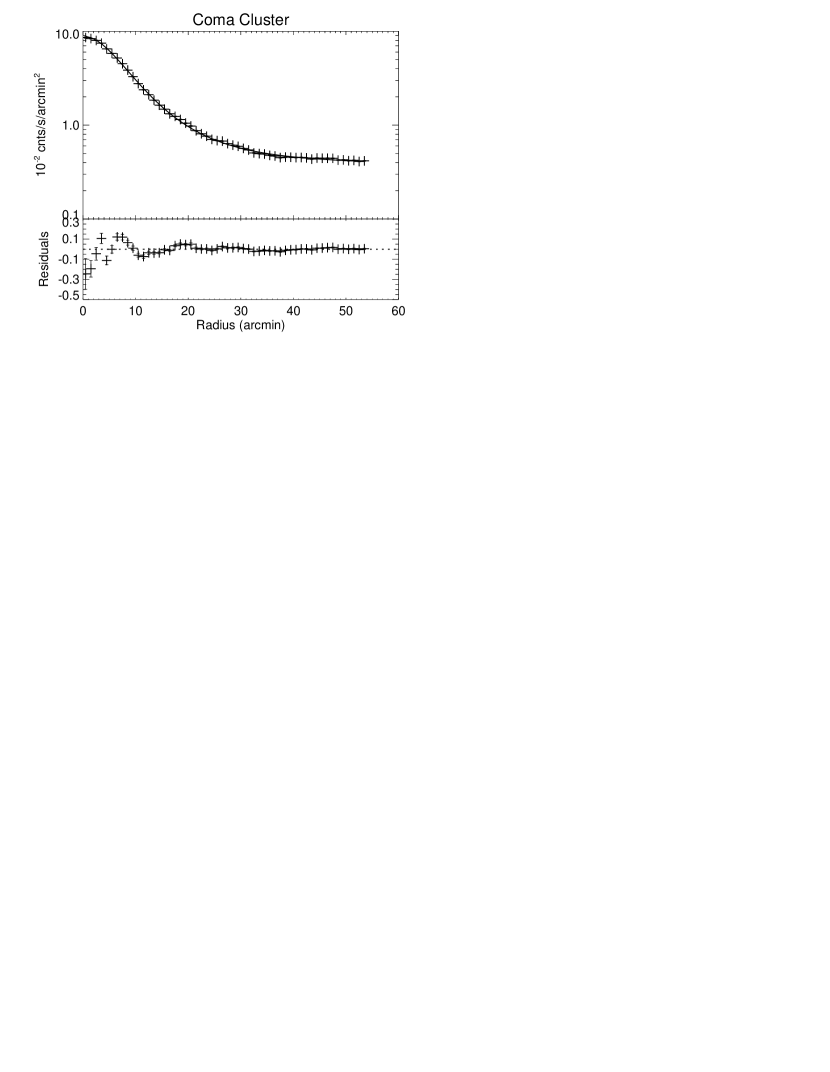
Figure 1: Isothermal $\beta$-model (Eq. 1) fits to the ROSAT X-ray surface brightness data of the Bonamente et al sample of clusters. The ROSAT mission was chosen because of its wide field-of-view, which allows one to determine clearly the surrounding background level even for the larger clusters. For non-isothermal ‘cooling flow’ clusters the central region where the phenomenon occurs is excluded from our analysis.

For ‘cooling flow’ clusters, the central region where cooling occurs is excluded from the modeling. The repercussions of such a procedure are discussed at length in section 5, where high resolution XMM-Newton data will be used to demonstrate that any errors in the SZE associated with this analysis method are too small to affect our final conclusions. All the ROSAT radial profiles of the member clusters of the Bonamente sample are shown in Figure 1. The best-fit $\beta$-model parameters, together with other essential details of each cluster, are to be found in Table 1, where a spot check against Briel & Henry (1996) reveals reasonable agreement with their values of $n_{0}=$ 3.15 $\pm$ 0.29 $\times$ 10^-3 cm^-3, $\theta_{c}=$ 5.15 $\pm$ 0.46 arcmin, and $\beta=$ 0.93 $\pm$ 0.04 for A1795.

The predicted SZE decrement as a function of angle relative to the cluster center direction is then given by

$$\frac{\Delta T_{{\rm SZ}}(\theta)}{T_{{\rm CMB}}}=\frac{kT}{m_{e}c^{2}}\sigma_{{\rm Th}}\int dl~{}n_{e}\left[\frac{x(e^{x}+1)}{e^{x}-1}-4\right],$$ (2)

where $x=h\nu/kT_{{\rm CMB}}$ with $\nu$ being the mean frequency of the WMAP observing filter, $\sigma_{{\rm Th}}$ is the Thomson cross section, $l$ is the pathlength through the cluster along our off-axis sightline, and the electron density is

$$n_{e}(r)=n_{0}\left[1+\left(\frac{r}{r_{c}}\right)^{2}\right]^{-\frac{3\beta}{2}},$$ (3)

with $r=r(l,\theta)$ being the radius. The integration of Eq. (2) was performed analytically by previous authors, resulting in an expression for $\Delta T_{{\rm SZ}}(\theta)/T_{{\rm CMB}}$ which depends on $n_{0}$, $\beta$, and the core radius $r_{c}=L\theta_{c}$ where $L=cz/H_{0}$ (with $H_{0}=$ 71 km s^-1 Mpc^-1) is the distance to a nearby cluster, see e.g. Refregier, Spergel, & Herbig (2000). We will not repeat these earlier calculations, except to say that upon application of our Coma cluster $\beta$-model parameters to the analytical formula we obtained $\Delta T_{{\rm SZ}}(\theta=0)/T_{{\rm CMB}}\approx-$590 $\pm$ 170 $\mu$K at the WMAP frequency of $\nu=$ 41 GHz. This compares well with the estimate by other groups, such as the value of $\Delta T_{{\rm SZ}}(\theta=0)/T_{{\rm CMB}}\approx-$507 $\pm$ 92.7 $\mu$K at 32 GHz as obtained by Herbig, Lawrence, & Readhead (1995).

3. The cluster WMAP temperature profiles; effect of the point spread function

To examine whether the WMAP mission detected temperature variation in the fields of the Bonamente sample we extracted ‘thumbnail’ images (small maps) from the WMAP first year database centered at the X-ray centroids of the 38 clusters, i.e. the coordinates as listed in Table 1. Clusters with bright radio sources along their sightlines (Virgo, A21, A1045) are excluded from further analysis. In addition, Fornax, A1314, and A1361 were excluded due to difficulties in estimating the uncertainty in the X-ray brightness distribution. Lastly, Hercules was not considered because the exact location of the cluster emission could not be identified unambiguously. For the remaining 31 sample members radial profiles of the mean temperature deviation over concentric annuli are computed after removing the dipole and quadrupole components, and plotted in Figure 2, where the error bars for each radius interval reflect an antenna noise which scales as the inverse-square-root of the number of observations of the sky area. We restrict attention to the cosmological bands of Q, V and W, since the K and Ka bands are dominated by Galactic foreground emissions and absorptions (Bennett et al 2003a,b).

In order to compare any spatial features seen at a cluster position with the expected SZE behavior, it is necessary to take into account the WMAP point spread function (PSF). For each of the three filters we computed the average brightness profile from 15 point sources and fitted it with a Gaussian function as shown in Figure 3. It was possible to perform the averaging of these profiles because they all compare well with each other statistically, even though the sources are located at very different parts of the sky, with the highest being at Galactic latitude $|b|\approx$ 74^o. This indicates that the performance of WMAP in spatially resolving CMB temperature variations is consistent across the sky. The SZE profile of each cluster as inferred from Eq. (2) and Table 1 is convolved with the PSF of the appropriate filter. A test of the correctness of our procedure was done by adopting the $\beta$-model in Figure 1(c) of Myers et al (2004). After convolving this model with the W-band PSF, our results are plotted in Figure 4. It bears close resemblance to the corresponding profile in the Myers paper.

With the assurance of the aforementioned cross-checks the expected SZE decrement for each cluster is seen overplotted in Figure 2, where the unperturbed ‘continuum’ is aligned with the average temperature deviation in the outermost (2^∘ - 3^∘) annulus. The co-added model and data profiles for each filter is shown in Figure 5. In all plots the error bars for each radius interval reflect an antenna noise which scales as the inverse-square-root of the number of observations of the sky area. An analysis of the (radial) bin-to-bin variation of the profile of many co-added random fields reveal that the degree of relative fluctuation between neighboring radial bins is in accordance with the size of the error bars as shown in Figure 5 for each bin. This enables us to evaluate the formal statistical significance of the overall detection of a broad temperature decrement feature in the composite radial profiles as 9$\sigma$, 4.2$\sigma$, and 2.3$\sigma$ for the Q, V, and W band respectively (see Figure 5 for more details). Note that the true significances are likely to be less than those given by the three numbers, because systematics effects in the WMAP data were not included when we calculated them. Such effects will be discussed at length in the next section.

4. Systematic CMB temperature variation from WMAP random fields

From the graphs in Figure 2, a broad CMB temperature decrement positionally coincident with the cluster and of commensurate spatial extent as the cluster size is apparent for some clusters, such as Coma, A1795, A1413, A2199, A2219, and A2255. On the other hand, there are clearly counter examples like A85, A1367, A1689, A2029, A3301, A3558, and A3571. There are also clusters that fall within a ‘grey’ zone where no judgment can be made at all. Apart from some clusters having small expected SZE amidst poor signal-to-noise, another key problem that weakens any verdict from an individual cluster is the ambiguity in the CMB temperature ‘continuum’ appropriate to the observation. In fact, we are dealing with a non-trivial systematic uncertainty which can only be understood by examining many randomly chosen fields across the WMAP sky with $|b|\geq$ 30^o. For this reason we constructed radial profiles for 100 of such fields.

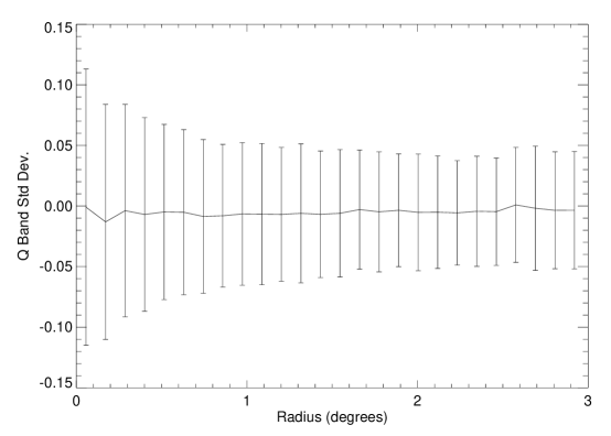
Figure 6: The r.m.s. field-to-field variation of CMB temperature at a given radial interval, and for the Q, V, W bands of WMAP, as obtained by comparing the radial profile 100 random pointings.

A plot of the r.m.s. variation (from one random field to another) of the temperature difference at each radial interval is shown in Figure 6, where it is evident that systematic effects at the level of 0.1 mK are commonplace among the smaller radius annuli. To be even more specific, we display in Figure 7 the radial profiles of four random fields. It can be seen that degree-scale modulations are frequently present, with an amplitude of $\approx$ 0.1 mK, often found at the $\theta=$ 0 (i.e. on-axis) position. The phenomenon pertains to the most prominent fluctuation in the WMAP data - the primary acoustic peak - which has an amplitude of $\Delta T_{{\rm CMB}}\approx$ 0.1 (or $\Delta T_{{\rm CMB}}/T_{{\rm CMB}}\approx$ a few $\times$ 10^-5, see Bennett et al 2003b). Thus, when a single cluster field exhibits some broad central ‘bump’ it is not necessarily the signature of an emission source; in fact we shall demonstrate that for our cluster sample as a whole the discrepancy between predicted and detected SZE profiles cannot be due to line-of-sight emissions. Likewise, the existence of a central trough may also be caused by primordial acoustic oscillations rather than the SZE. The only way of knowing whether there is consistency between the WMAP data and cluster SZE’s is to examine the co-added profiles of all the clusters, when the systematic effects which prevent one from determining the ‘continuum’ level can largely be suppressed.

In order to be certain that the temperature does stabilize among co-added fields we generated average radial profiles of 33 random fields at a time (Figure 8). If the primary acoustic peaks and troughs are stacked with arbitrary central alignment in this way, one would expect the fluctuation amplitude to be reduced from the $\sim$ 0.1 mK value by a factor of $\approx\sqrt{30}$, to about 0.02 mK. This is completely borne out by our averaged random profiles, which also indicate that towards the larger (2^∘ – 3^∘) annuli the CMB temperature deviations from the global mean value are very uniform, hovering close to zero. By the time 100 randomly generated profiles are averaged, the data points are smooth throughout all radii (Figure 8). With the help of these plots (of the merged 100 fields), wherein the systematic variations are no longer a problem, we could verify if the error bar on each radial bin (antenna random noise) is independent of other bins. The answer is yes, because the r.m.s. scatter among the data points is found to be consistent with the size of the error bars.

Returning now to the averaging of 33 random fields, Figure 8, the residual systematic excursions in the data are important towards understanding the radial profile of the co-added cluster fields, Figure 5. This is because both Figures involve the stacking of a similar number of WMAP fields. Since the magnitude of any remaining systematic effect is, as can be seen in Figure 8, far less than the discrepancy between observed and expected SZE in our cluster sample, Figure 5, one must conclude that the apparent incomplete SZE is not due to intrinsic sky variations in the CMB temperature recorded by WMAP, i.e. it is a genuine anomaly that deserves an explanation.

5. Interpretation

How can one reconcile a cosmological CMB origin with Figure 5? It is perhaps more reasonable to first examine whether, despite many generations of X-ray observatories measuring the X-ray properties of clusters, we are still misled by uncertainties on the hot ICM parameters? Then there is the question of radio source contamination also.

Could a steepening in the slope of the hot ICM density profile beyond the radius where the $\beta$-model is well constrained by ROSAT data lead to an overestimation of the SZE? We pause to consider an extreme scenario under which the WMAP’s spatial resolution is so poor that the entire SZE of even a nearby cluster simply appears as a ‘point sink’ at zero radius. If this is really the case, the WMAP radial profile of the SZE would have the shape of the PSF, with the flux within the entire profile being equal to the cluster SZE integrated over all sightlines cutting through the cluster at various ‘impact parameters’. For a $\beta$-model, however, this total flux is dominated by the SZE at the outer radii where the model is no longer well constrained by the X-ray data. The reason is that at any off-axis angle $\theta$ the line-of-sight SZE has the form:

$$\Delta T_{{\rm SZ}}(\theta)=\Delta T_{{\rm SZ}}(0)\left[1+\left(\frac{\theta}{\theta_{c}}\right)^{2}\right]^{-\frac{3\beta}{2}+\frac{1}{2}}.$$ (4)

At least for our sample of clusters ROSAT data fail to guide the model only at radii $\theta\gg\theta_{c}$, and typically at $\theta>$ 10 arcmin in real units.

The total X-ray predicted SZE, integrated over all values of $\theta$, is dominated by the values of $\Delta T_{{\rm SZ}}(\theta)$ in the range $\theta\gg\theta_{c}$, unfortunately. This is because

$$\Delta T_{{\rm SZ}}^{{\rm total}}=\int_{0}^{\infty}\Delta T_{{\rm SZ}}(\theta)~{}2\pi\theta d\theta,$$ (5)

and for $\theta\gg\theta_{c}$ the integral $\sim\theta^{-3(\beta-1)}$, which diverges at the upper integration limit because the inequality $\beta<$ 1 applies to our clusters (see Table 1). In fact, from Eq. (3) it can also be seen that the total cluster mass, proportional to $\int n_{e}(r)r^{2}dr$, scales with the upper cutoff radius in exactly the same way. Thus the outcome of our analysis is that if WMAP’s spatial resolution is very poor the X-ray model can overpredict the SZE by an arbitrarily large amount. This point was already raised in the recent papers of Benson et al (2004) and Schmidt, Allen, and Fabian (2005). Specifically, while Schmidt, Allen, and Fabian (2005) reported a steepening in the slope of the $\beta$-model (i.e. less hot ICM) towards a cluster’s outskirts by comparing Chandra and ROSAT data, Benson et al (2004) found that provided the SZE is evaluated over a radius commensurate with the resolution (or beam size) of the instrument any difference among the predictions derived from the various sets of model parameters actually remains small.

In the context of this last point of Benson et al (2004), we shall demonstrate that most of the results we obtained in the previous sections remain robust: the WMAP resolution is not as pessimistic as that depicted in the extreme scenario we just considered, because the detected SZE profiles are much wider than the instrument PSF. In fact, much of the SZE within the central 0.5^∘ radius of ‘matching’ with the WMAP beam is not due to the PSF leaking signals from large radii inwards. Instead the opposite is true: there is a loss of inner signals outwards which only widens the actual gap between SZE prediction and observation. To test these statements, we chose a pair of $\beta$-model parameters typical to our cluster sample, viz. $\beta=2/3$ and $\theta_{c}=$ 2 arcmin, and truncate the full line-of-sight integrated SZE profile, Eq. (4), abruptly at $\theta=$ 10 arcmin, resulting in the following functional dependence:

$$\Delta T_{{\rm SZ}}^{{\rm cutoff}}(\theta)=\Delta T_{{\rm SZ}}(0)[1+0.25(\theta/{\rm arcmin})^{2}]^{-\frac{1}{2}}~{}{\rm for}~{}\theta\leq 10~{}{\rm arcmin};~{}{\rm and}~{}=0~{}{\rm otherwise.}$$ (6)

The reason for setting the cutoff at 10 arcmin is that for most of the clusters in our sample, Figure 1 indicates the ROSAT data can constrain the surface brightness profile out to at least such a radius. If, after convolution of the truncated profile with the PSF there is a significant reduction of the inner SZE, this would imply a severe flux overprediction problem at small radii by the WMAP PSF, which spreads signals inwards from regions beyond 10 arcmin where the $\beta$-model is no longer so reliable. Note that in our test we did not truncate the $\beta$-model self-consistently by reducing the line-of-sight integration to reflect the projection effect of the cutoff at $\theta\leq$ 10 arcmin. This is a separate question to be investigated below.

The outcome of the test is shown in Figure 9, where it can be seen that within $\theta\leq$ 0.5 arcmin the reduction in SZE by our truncation procedure is $\approx$ 12 % for the Q band, and much less for the V and W bands. This means any incorrectness in the outer (questionable) parts of the $\beta$-model, when coupled with the WMAP PSF spreading effect, cannot lead to an overprediction of the SZE within the central 0.5 arcmin radius by a factor of four to six. Yet such factors are necessary to explain the average discrepancy between X-ray expectation and WMAP observed SZE levels for the three cosmological filter passbands, see Figure 5. We must also point out that in terms of PSF effects the real problem is the opposite, viz. the loss of inner signals to the radii beyond, as borne out by the fact that when we convolved $\Delta T_{{\rm SZ}}^{{\rm cutoff}}(\theta)$ with the PSF and compared the total SZE over $\theta\leq$ 10 arcmin with the same quantity obtained before convolution, the ratio of the latter to the former ranges from 2.48 (Q band) through 5.31 (V band) to 5.61 (W band). Since the average X-ray predicted SZE profile is more centrally peaked than the WMAP observed profile, Figure 5, this means the discrepancy between ROSAT and WMAP should have been even more pronounced if the original intrinsic profiles before PSF convolution were compared.

In order to assess the line-of-sight projection effect of the outer parts of the $\beta$-model on the inner SZE prediction, we may e.g. divide the central decrement $\Delta T_{{\rm SZ}}(0)$ into two parts, respectively contributions from the hot ICM within and beyond the truncation limit of $\theta=\theta_{T}=$ 10 arcmin, i.e. we write

$$\Delta T_{{\rm SZ}}(0)\propto\int_{0}^{\theta_{T}}\left[1+\left(\frac{\theta}{\theta_{c}}\right)^{2}\right]^{-\frac{3\beta}{2}}d\theta+\int_{\theta_{T}}^{\infty}\left[1+\left(\frac{\theta}{\theta_{c}}\right)^{2}\right]^{-\frac{3\beta}{2}}d\theta.$$ (7)

For our typical sample parameters of $\beta=$ 2/3 and $\theta_{c}=$ 2 arcmin the ratio of the 2nd term on the right side to the first term is 14.5 %. It is clearly not of a magnitude large enough to explain the discrepancy of concern, which is at the 400 – 600 % level (Figure 5). The same conclusion may be drawn about the other slightly off-axis sightlines of the innermost 0.5^∘ radius.

The impact of uncertainties in the X-ray $\beta$-model on the integrity of the present work may quantitatively be summarized into two points. Firstly, we can calculate the significance of the average discrepancy between the predicted and observed SZE as depicted in Figure 5, taking into account: (a) the random error bars shown in Figure 5 (i.e. antenna noise for each radial bin, see the end of section 3); (b) the systematic error per bin which is also shown in Figure 5 and described in section 4; (c) the uncertainty in the $\beta$-model parameters manifested as errors in the model prediction for each bin, shown in Figure 5 as the vertical interval between the dashed and solid lines; and (d) systematic error in the $\beta$-model prediction for the inner radial bins due to unreliability of the model at the cluster outskirts coupled with the WMAP PSF smearing effect, as described in this section and quantified in Figure 9. When all four error components are added in quadrature, we find that for the central 1 arcmin radius the discrepancy between prediction and observation has the significance level of 2.73 $\sigma$, 4.65 $\sigma$, and 4.70 $\sigma$ respectively for the Q, V, and W band. This level becomes even higher if the next few bins are also included with our calculation.

Onto our second summary point. As was argued earlier, since the total SZE summed over all sightlines out to some limiting radius $\theta\gg\theta_{c}$ scales with $\theta$ as the total hot ICM mass (out to the same radius) does, we used Figure 5 to compute an ensemble average over our 31 member cluster sample the ratio of the X-ray predicted to WMAP observed total SZE out to $\theta=$ 10 arcmin (i.e. $\theta\gg\theta_{c}\approx$ 2 arcmin). This ratio, which ranges from 1.49 (Q band) through 2.21 (V band) to 2.82 (W band), indicates by how much must the X-ray $\beta$-model estimate of the hot ICM mass within the radius $\theta=$ 10 arcmin be reduced in order to secure a match between ROSAT and WMAP. For the W band, which is the best (cleanest) cosmological filter of WMAP, the answer is close to 300 %. It is somewhat surprising that the $\beta$-model can lead to such large errors in the X-ray gas mass: errors which effectively deemed many previous X-ray observations of the hot ICM as meaningless. Note also that, as already explained, because the X-ray predicted SZE profile is more centrally peaked than the WMAP profile, problems with the leakage of flux towards the $>$ 10 arcmin radii by the WMAP PSF render the correct percentage reduction of the hot ICM mass even higher than 300 %.

Could a ‘cooling flow’ which exists in some clusters invalidate any estimate of central SZE based upon isothermal $\beta$-model fits to the ROSAT data? While remaining in the spirit of the foregoing discussion, viz. on the question of how the SZE predicted profile for the central 0.5^∘ radius of ‘matching’ with the WMAP beam may be affected by the on-axis flux decrement, we turn to the possible role played by the cooling of cluster cores. By using the more accurate measurements of Chandra, Schmidt, Allen, and Fabian (2005) found that a straightforward ROSAT $\beta$-model inference of $\Delta T_{{\rm SZ}}(0)$ could lead to an overestimate of the quantity by less than a factor of two. Apart from re-emphasizing that the WMAP observations are more discrepant from our X-ray predictions than by this factor, it must also be stressed that the ROSAT $\beta$-model we employed are derived by fitting only the ROSAT data from regions lying beyond ‘cooling flow’ radii. Thus, while it is true that the central cooling of the hot ICM causes $\Delta T_{{\rm SZ}}(0)$ to decrease, any accompanying central peaking of the gas density which has not been taken into account by the $\beta$-model has the opposite effect. The net outcome depends on how the product $n_{e}(r)kT(r)$, i.e. the gas pressure, scales with radius relative to the $\beta$-model inferred without taking the ‘cooling flow’ into account. After investigating our present sample, we found that ‘cooling flows’ tend to maintain or raise the $y_{0}$ parameter rather than lower it. We illustrate this point by showing in detail the situation of A2029, a cluster over which the discrepancy between WMAP and ROSAT is large (see Figure 2). For this cluster the product $n_{e}(r)kT(r)$ is constrained using the high resolution data of XMM-Newton, and its deprojected radial profile as plotted in Figure 11 is shown to compare closely with the $\beta$-model of Table 1 for A2029.

Could line-of-sight non-CMB emissions have contaminated the WMAP passbands? In the restricted venue of the center of the Coma cluster Herbig, Lawrence, & Readhead (1995) measured a SZE of -270 $\mu$K when the prediction is $\approx$ -500 $\mu$K. The authors attributed the discrepancy to radio sources located along the central sightline but not members of the cluster. If, in general, line-of-sight sources unrelated to the clusters are bright enough to affect the WMAP data, the phenomenon should also be present among non-cluster directions, i.e. one should expect the same level of contamination to exist in the WMAP random fields. There is however no evidence for this, because the radial profiles of the $\sim$ 30 accumulated random fields reveal an average temperature deviation of $\approx$ 0.005 mK for the three cosmological bands of Q,V, and W (see Figure 8), which is on par with the average asymptotic deviation among the co-added cluster fields. Moreover, such amounts are far less than the discrepancy between the predicted and observed SZE of Figure 5.

Could the clusters themselves be a significant source of emission in the WMAP passbands? There are two possibilities. Diffuse emission from cosmic ray synchrotron radiation and discrete radio sources. The former is in principle a possibility (e.g. Sarazin & Lieu 1998), and we are currently investigating it, but see the two paragraphs after next. Concerning the latter, one can get a good idea of the cluster radio source occurence probability by appealing to the Owens Valley radio interferometry survey (Bonamente et al 2005), which finds on average approximately one radio source per cluster with $\sim$ 1 mJy brightness at 30 GHz. Since the Owens Valley sample is more distant than ours, with a mean separation of $\sim$ 1.5 Gpc as opposed to $\sim$ 0.5 Gpc for our present sample, the brightness level should scale to 10 mJy, or 10^-28 W m^-2 Hz^-1. Since, to reduce the SZE by invoking emission components, such components must account for an average CMB temperature increase of $\delta T_{{\rm CMB}}\approx$ 5 $\times$ 10^-5 K distributed over the area of 0.5^∘ angular radius.

Is the equivalent of one unresolved 10 mJy source within the same area sufficient? The conversion from $\delta T_{{\rm CMB}}$ to a change in the observed flux involves multiplying the Rayleigh-Jeans sky flux $2\pi k\delta T_{{\rm CMB}}\nu^{2}/c^{2}$ by the solid angle factor $\delta\Omega/4\pi$ where $\delta\Omega=\pi\theta^{2}$ with $\theta=$ 0.5^∘. This yields an excess flux at $\nu=$ 30 GHz of 10^-27 W m^-2 Hz^-1, ten times higher than the contribution from cluster radio sources. Such a conclusion is applicable to the Q band, which measures at a frequency only slightly higher than 30 GHz. For the W band, at a frequency of 94 GHz, the radio source contribution is at least two orders of magnitude short, because such sources typically have flux spectra $F_{\nu}\sim\nu^{-\alpha}$ where $\alpha\geq$ 2.

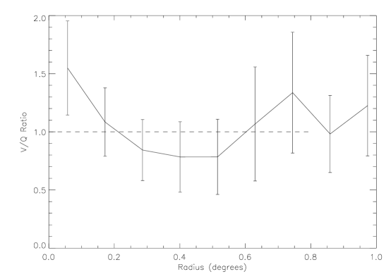
Figure 10: Radial profile of the filter ratio of the temperature discrepancy between SZE model and data, for the 31 co-added cluster fields of Figure 5. First plot gives V:Q ratio, second is V:W, and third is W:Q. If the missing flux responsible for the discrepany has a black body spectrum, the filter ratios will equal unity.

Since any cluster emissions which may account for the less than expected SZE detection by WMAP, be they diffuse or discrete in form, are invariably non-thermal in nature, with a flux spectrum $F_{\nu}\sim\nu^{-2}$ or steeper, i.e. a very different spectral shape from the Rayleigh-Jeans $F_{\nu}\sim\nu^{2}$ dependence, another test would involve checking the WMAP band ratios of the SZE discrepancy. Thus a cluster source is distinguished by its larger V to W band flux ratios, which even in the case of a power-law as shallow as $F_{\nu}\sim\nu^{-0.5}$, is a factor of three more than the corresponding ratio for Rayleigh-Jeans spectra. Since the observed ratio of V:W for any extra radiation component that may account for the discrepancy in Figure 5 is close to the black body limit, see Figure 10, we conclude that the resolution does not lie with discrete cluster radio sources.

In addition to the above, there is one more powerful test. If clusters do exhibit a normal SZE which is masked by self emissions unrelated to the hot ICM, one would expect additional field-to-field variation of the CMB temperature at a given radial bin within our cluster sample, because the properties of the hot ICM and non-thermal radiation vary from cluster to cluster. At the very minimum, the r.m.s. fluctuation must equal that of the blank field and the differing degree of SZE from one hot ICM to the next, with the two effects added in quadrature. That even this minimum is already less than the observed r.m.s. within our cluster sample is depicted in Figure 12. In fact, the observed r.m.s. is at the same level as that of the blank fields, excluding not only non-thermal emissions, but also the SZE itself, unless one contrives a scenario in which the two are correlated with each other.

Could peculiarities in the hot ICM abundance, or the gradual decline of the hot ICM temperature with radius be responsible? The general reasoning can always be applied, especially at the centers of clusters where physics are more complicated, to argue that if there are bright and spectrally unresolved metallic lines the density of the hot ICM electrons, which is ordinarily determined by assuming that over most the X-ray passband the emission is a continuum, may drop, resulting in a reduction of the expected SZE. In reality, however, the effect is very small. Thus e.g. in the case of A2029, the hot ICM abundance originally used by us to calculate the SZE was 0.3 solar. Analysis of XMM-Newton data revealed the same abundance level, Figure 11, hence no change in the density of hot ICM electrons. As to the large scale radial temperature decline, numerical simulation of clusters (Romeo et al 2005) indicates that the hot ICM temperature can be halved by the time one reaches the virial radius. Observationally, however, it is clear that at least out to the radius $R=5r_{c}$ beyond which the hot ICM contribution of the SZE is negligible (see Eq. (7)), there is no evidence for such a temperature drop. For instance, in the case of A2029 which has a core radius of 2 arcmin, the hot ICM temperature as measured by XMM-Newton (Figure 11) remains stable out to 10 arcmin. Thus the cooling of the hot ICM towards the cluster’s outskirts is not the reason for the large discrepancy between WMAP and X-ray fluxes.

On the role of asphericity of either the central core or the entire cluster, and clumpiness of the hot ICM, these questions are harder to answer quantitatively. Given that we averaged over 31 clusters, however, any residual asphericity corections must be very small, unless one contrives a scenario under which clusters have their major axes aligned along some preferred direction. Clumpiness is a phenomenon worthy of further research, because (to argue heuristically) while the X-ray observations measure $\langle n^{2}_{e}\rangle$ the SZE probes $\langle n_{e}\rangle$. The two are trivially related to each other if $\langle n_{e}\rangle^{2}=\langle n^{2}_{e}\rangle$, which occurs only when the gas is smooth. Once clumps are present, $\langle n^{2}_{e}\rangle>\langle n_{e}\rangle^{2}$, so the X-ray prediction will overestimate the SZE flux. Although for the hot ICM beyond the central core it is difficult to envisage, from pressure balance considerations, how such high temperature plasmas could exhibit a large degree of clumping, the situation may be different within the core itself where the cooling of gas and other dynamic processes often occur. It would still be surprising if the factor of six discrepancy reported here for the W-band could entirely be attributed to this effect. Nevertheless, in the absence of further observational evidence, or a sound physical argument, one should not exclude the scenario of hot ICM clumping as possible cause of our reported discrepancy.

Finally, one could ask if photon populations other than the CMB may exist to interact with the hot ICM electrons to ‘refill’ the SZE flux. Whether we are dealing with ‘upward’ or ‘downward’ scattering, the difficulty lies with insufficient seed photon flux at frequencies well below and above the WMAP passbands. This is the reason for the general belief that cluster SZE should cause a clean removal of the CMB from its original microwave passband of emission.

Conclusion

Formally, a statistically significant detection of the SZE across our entire cluster sample was achieved by WMAP. The level of this detection is very weak, however. Not only is the field-to-field variation of the CMB temperature within the sample (due to different clusters exerting unequal SZE on the CMB) non-existent, Figure 12, but also the measured decrements of Figure 5 are consistent with nothing beyond the usual primary CMB anisotropy, viz. the systematic variations in the CMB average radial profile for a commensurate number of co-added blank (random) fields, Figure 8. Of particular concern are the data of the W-band, which is the passband containing the cleanest extragalactic signals (Bennett et al 2003b). The statistical significance of an overall W-band SZE detection is $<$ 3 $\sigma$, when the expected effect is far larger. Here we also note that a similar shallow decrement was seen in the Myers et al. (2004) paper where the best fit model had a $\Delta T_{0}$ of 0.083 mK in the W band. This is much smaller than the predicted average decrement from our sample of 0.46 mK from Table 1. Thus, taken at value one may even hold the opinion that there is in fact no strong evidence in the WMAP database for the SZE at all, when the aggregate behavior of all the clusters in the sample, rather than individual cases, is considered.

Naturally the entire premise of this paper depends on the reliability of the original WMAP data. If there are any data analysis issues with the WMAP processing that can explain the extra diffuse emission seen in our SZE clusters then our findings will be obsolete. However, this would have implicate severely all the WMAP analysis done to date. One possible resolution is to look at the SZE as probed using dedicated ground based observatories. The SZE has already been detected in a large number of high-redshift clusters using interferometric techniques of higher resolution than the WMAP data (e.g., Carlstrom et al. 1996; Joy et al. 2001; Reese et al. 2002; Bonamente et al. 2005; LaRoque et al. 2005). Comparison of radio interferometry and X-ray data for the same clusters show that SZE-derived and X-ray derived masses and gas fractions are in agreement (Grego et al. 2001; LaRoque et al. 2005), and allows for a determination of the cosmic distance scale (Reese et al. 2002; Bonamente et al. 2005). There is not necessarily a conflict between our present results and the previous reported SZE detections for individual clusters. As can be seen from Figure 2, many of the clusters in our sample do exhibit the effect at $\sim$ the anticipated level.

In summary, it is through the first detailed radial profile comparison between X-ray and microwave observations that an apparent sample-wide discrepancy between the expected and measured levels of SZE from some of the best known clusters of galaxies was uncovered. The difficulty lies with the average behavior of our randomly selected cluster sample, which could still be suffering from systematic yet hitherto unknown biases. Nonetheless, the average CMB temperature decrement is sufficiently shallow to be interpreted simply as the usual primary CMB anisotropy: there is no need to invoke any SZE at this stage of the WMAP analysis.

We are grateful to an anoymous referee for comments and critique of this work.

Table 1: X-ray properties of the 31 clusters employed for the present SZE investigation. The $\beta$-model parameters are derived from ROSAT observations.

Name	Galactic (2000)		Redshift	kT	n0	$\beta$	Rcore	$\Delta T0_{Q}$	$\Delta T0_{V}$	$\Delta T0_{W}$	CF?
	Long.	Lat.		(keV)	$\times 10^{-3}$ cm-3		(arcmin)	mK	mK	mK
Abell 85	115.053	-72.064	0.055	7.0	$15.17^{+0.30}_{-0.40}$	$0.58^{+0.03}_{-0.04}$	$1.8^{+0.5}_{-0.9}$	$-0.99_{-0.30}^{+0.49}$	$-0.94_{-0.28}^{+0.46}$	$-0.81_{-0.24}^{+0.40}$	Yes
Abell 133	149.761	-84.233	0.057	5.0	$3.33^{+0.14}_{-0.13}$	$0.72^{+0.09}_{-0.07}$	$3.4^{+0.8}_{-0.8}$	$-0.22_{-0.06}^{+0.06}$	$-0.20_{-0.06}^{+0.06}$	$-0.18_{-0.05}^{+0.05}$	Yes
Abell 665	149.735	34.673	0.1816	7.0	$3.34^{+0.19}_{-0.23}$	$0.64^{+0.10}_{-0.10}$	$1.3^{+0.1}_{-0.1}$	$-0.40_{-0.14}^{+0.08}$	$-0.38_{-0.14}^{+0.08}$	$-0.33_{-0.12}^{+0.07}$	No
Abell 1068	179.100	60.130	0.139	5.0	$8.16^{+0.49}_{-0.43}$	$0.90^{+0.17}_{-0.13}$	$1.5^{+0.5}_{-0.5}$	$-0.43_{-0.16}^{+0.15}$	$-0.40_{-0.15}^{+0.15}$	$-0.35_{-0.13}^{+0.13}$	Yes
Abell 1302	134.668	48.904	0.116	4.8	$2.88^{+0.19}_{-0.15}$	$0.64^{+0.12}_{-0.08}$	$1.4^{+0.4}_{-0.3}$	$-0.17_{-0.07}^{+0.05}$	$-0.16_{-0.06}^{+0.05}$	$-0.14_{-0.05}^{+0.04}$	$\cdots$
Abell 1314	151.828	63.567	0.0341	5.0	$1.00^{+0.27}_{-0.26}$	$0.35^{+0.21}_{-0.10}$	$2.6^{+3.2}_{-2.4}$	$-0.44_{nan}^{+0.58}$	$-0.42_{nan}^{+0.55}$	$-0.36_{nan}^{+0.47}$	No
Abell 1361	153.292	66.581	0.1167	4.0	$2.81^{+nan}_{-0.73}$	$1.78^{+18.23}_{-1.08}$	$5.2^{+34.0}_{-4.1}$	$-0.19_{nan}^{+0.22}$	$-0.18_{nan}^{+0.21}$	$-0.16_{nan}^{+0.18}$	Yes
Abell 1367	234.799	73.030	0.0276	3.5	$1.68^{+0.03}_{-0.03}$	$0.52^{+0.02}_{-0.02}$	$8.6^{+0.5}_{-0.6}$	$-0.17_{-0.02}^{+0.02}$	$-0.16_{-0.02}^{+0.02}$	$-0.14_{-0.02}^{+0.01}$	uncertain
Abell 1413	226.182	76.787	0.143	6.0	$13.85^{+0.78}_{-0.94}$	$0.68^{+0.11}_{-0.11}$	$1.1^{+0.1}_{-0.1}$	$-0.91_{-0.29}^{+0.18}$	$-0.86_{-0.28}^{+0.17}$	$-0.74_{-0.24}^{+0.14}$	No
Abell 1689	313.387	61.097	0.181	7.0	$14.02^{+0.76}_{-0.90}$	$0.75^{+0.12}_{-0.12}$	$1.0^{+0.0}_{-0.0}$	$-1.01_{-0.28}^{+0.17}$	$-0.96_{-0.26}^{+0.16}$	$-0.83_{-0.23}^{+0.14}$	No
Abell 1795	33.788	77.155	0.061	7.0	$3.05^{+0.04}_{-0.06}$	$0.99^{+0.04}_{-0.06}$	$5.2^{+0.3}_{-0.4}$	$-0.33_{-0.03}^{+0.03}$	$-0.32_{-0.03}^{+0.03}$	$-0.27_{-0.02}^{+0.02}$	Yes
Abell 1914	67.196	67.453	0.171	9.0	$13.34^{+0.23}_{-0.21}$	$0.85^{+0.04}_{-0.04}$	$1.4^{+0.1}_{-0.1}$	$-1.47_{-0.12}^{+0.12}$	$-1.39_{-0.12}^{+0.11}$	$-1.20_{-0.10}^{+0.10}$	$\cdots$
Abell 1991	22.762	60.497	0.0586	4.0	$3.18^{+0.56}_{-0.35}$	$0.82^{+0.54}_{-0.22}$	$2.8^{+2.8}_{-8.4}$	$-0.12_{-0.14}^{+0.37}$	$-0.12_{-0.13}^{+0.35}$	$-0.10_{-0.11}^{+0.30}$	Yes
Abell 2029	6.505	50.547	0.0767	9.0	$13.54^{+0.21}_{-0.92}$	$0.67^{+0.03}_{-0.11}$	$1.9^{+0.3}_{-0.3}$	$-1.27_{-0.44}^{+0.23}$	$-1.21_{-0.42}^{+0.21}$	$-1.04_{-0.36}^{+0.18}$	Yes
Abell 2142	44.213	48.701	0.09	9.0	$7.09^{+0.40}_{-0.48}$	$0.68^{+0.11}_{-0.11}$	$2.4^{+0.2}_{-0.3}$	$-0.98_{-0.32}^{+0.21}$	$-0.93_{-0.30}^{+0.20}$	$-0.80_{-0.26}^{+0.18}$	Yes
Abell 2199	62.897	43.697	0.0302	4.5	$6.87^{+0.08}_{-0.23}$	$0.65^{+0.02}_{-0.05}$	$3.1^{+0.5}_{-2.5}$	$-0.23_{-0.05}^{+0.19}$	$-0.22_{-0.05}^{+0.18}$	$-0.19_{-0.04}^{+0.16}$	Yes
Abell 2218	97.745	38.124	0.171	6.0	$3.00^{+0.17}_{-0.20}$	$0.72^{+0.12}_{-0.12}$	$1.5^{+0.1}_{-0.1}$	$-0.27_{-0.08}^{+0.05}$	$-0.26_{-0.08}^{+0.05}$	$-0.22_{-0.07}^{+0.04}$	uncertain
Abell 2219	72.597	41.472	0.228	7.0	$6.12^{+0.14}_{-0.13}$	$0.78^{+0.05}_{-0.04}$	$1.8^{+0.2}_{-0.1}$	$-0.88_{-0.10}^{+0.09}$	$-0.83_{-0.10}^{+0.09}$	$-0.72_{-0.08}^{+0.08}$	No
Abell 2241	54.784	36.643	0.0635	3.1	$11.66^{+0.48}_{-0.43}$	$0.74^{+0.09}_{-0.07}$	$1.0^{+0.2}_{-0.2}$	$-0.15_{-0.03}^{+0.03}$	$-0.14_{-0.03}^{+0.03}$	$-0.12_{-0.03}^{+0.03}$	$\cdots$
Abell 2244	56.772	36.306	0.097	7.0	$30.50^{+0.62}_{-1.00}$	$0.59^{+0.03}_{-0.04}$	$1.0^{+0.4}_{-0.9}$	$-1.72_{-0.71}^{+1.67}$	$-1.63_{-0.67}^{+1.58}$	$-1.41_{-0.58}^{+1.36}$	Yes
Abell 2255	93.975	34.948	0.08	7.0	$2.49^{+0.05}_{-0.05}$	$0.76^{+0.04}_{-0.04}$	$4.6^{+0.4}_{-0.3}$	$-0.40_{-0.04}^{+0.04}$	$-0.38_{-0.04}^{+0.04}$	$-0.33_{-0.03}^{+0.03}$	No
Abell 2256	111.096	31.738	0.06	7.0	$3.74^{+0.19}_{-0.23}$	$0.85^{+0.14}_{-0.14}$	$5.5^{+0.9}_{-0.9}$	$-0.48_{-0.14}^{+0.11}$	$-0.46_{-0.13}^{+0.10}$	$-0.39_{-0.11}^{+0.09}$	No
Abell 2597	65.363	-64.836	0.085	4.0	$18.94^{+0.79}_{-0.71}$	$0.69^{+0.08}_{-0.06}$	$1.2^{+0.7}_{-3.0}$	$-0.52_{-0.33}^{+1.37}$	$-0.49_{-0.31}^{+1.29}$	$-0.43_{-0.27}^{+1.12}$	Yes
Abell 2670	81.318	-68.516	0.076	3.0	$4.21^{+0.17}_{-0.18}$	$0.64^{+0.07}_{-0.06}$	$1.9^{+0.6}_{-0.8}$	$-0.14_{-0.05}^{+0.06}$	$-0.13_{-0.05}^{+0.06}$	$-0.12_{-0.04}^{+0.05}$	Yes
Abell 2717	349.076	-76.390	0.049	3.0	$9.41^{+0.21}_{-0.19}$	$0.64^{+0.04}_{-0.03}$	$1.5^{+0.2}_{-0.1}$	$-0.17_{-0.02}^{+0.02}$	$-0.16_{-0.02}^{+0.02}$	$-0.14_{-0.02}^{+0.02}$	$\cdots$
Abell 2744	8.898	-81.241	0.308	11.0	$3.12^{+0.23}_{-0.17}$	$1.60^{+0.44}_{-0.27}$	$3.3^{+0.6}_{-0.4}$	$-0.87_{-0.22}^{+0.19}$	$-0.82_{-0.21}^{+0.18}$	$-0.71_{-0.18}^{+0.15}$	No
Abell 3301	242.415	-37.409	0.054	7.0	$4.33^{+0.20}_{-0.18}$	$0.49^{+0.05}_{-0.04}$	$1.8^{+0.5}_{-0.4}$	$-0.39_{-0.15}^{+0.11}$	$-0.37_{-0.14}^{+0.11}$	$-0.32_{-0.12}^{+0.09}$	$\cdots$
Abell 3558	311.978	30.738	0.048	5.0	$2.65^{+0.04}_{-0.04}$	$0.79^{+0.04}_{-0.03}$	$5.9^{+0.4}_{-0.4}$	$-0.23_{-0.02}^{+0.02}$	$-0.22_{-0.02}^{+0.02}$	$-0.19_{-0.02}^{+0.02}$	Yes
Abell 3560	312.578	28.890	0.04	2.0	$4.96^{+0.23}_{-0.21}$	$0.49^{+0.05}_{-0.04}$	$2.6^{+0.6}_{-0.5}$	$-0.13_{-0.05}^{+0.04}$	$-0.13_{-0.05}^{+0.04}$	$-0.11_{-0.04}^{+0.03}$	$\cdots$
Abell 3562	313.308	30.349	0.04	4.5	$7.33^{+0.51}_{-0.64}$	$0.47^{+0.08}_{-0.08}$	$1.3^{+0.1}_{-0.1}$	$-0.26_{-0.26}^{+0.08}$	$-0.25_{-0.25}^{+0.08}$	$-0.22_{-0.21}^{+0.07}$	No
Abell 3571	316.317	28.545	0.04	7.0	$13.02^{+0.32}_{-0.30}$	$0.65^{+0.04}_{-0.04}$	$3.6^{+0.7}_{-0.7}$	$-1.05_{-0.23}^{+0.23}$	$-1.00_{-0.22}^{+0.22}$	$-0.86_{-0.19}^{+0.19}$	Yes
Abell 4059	356.833	-76.061	0.046	4.5	$5.03^{+0.45}_{-0.34}$	$0.99^{+0.30}_{-0.18}$	$6.0^{+2.2}_{-1.7}$	$-0.31_{-0.13}^{+0.11}$	$-0.29_{-0.13}^{+0.10}$	$-0.25_{-0.11}^{+0.09}$	Yes
Coma	58.080	87.958	0.023	8.2	$4.42^{+0.24}_{-0.29}$	$0.71^{+0.11}_{-0.11}$	$9.8^{+1.6}_{-1.6}$	$-0.59_{-0.20}^{+0.14}$	$-0.56_{-0.19}^{+0.13}$	$-0.48_{-0.16}^{+0.11}$	No

Figure 2: WMAP Q, V, and W band radial profiles of the CMB temperature deviation (from the all sky mean value) as averaged over concentric annuli centered at the positions of the 31 clusters employed in our analysis. The data were plotted after subtraction of the contribution from the CMB dipole and quadrupole anisotropy. The solid line gives the SZE temperature decrement profile expected from the hot ICM with properties determined by X-ray observations (including the ROSAT $\beta$-model of Figure 1) and displayed in Table 1. Dashed lines mark the 90 % error margin on the prediction, based upon uncertainties in the observed hot ICM parameters. The continuum level for the predicted SZE profile is fixed by aligning it with the average temperature deviation in the outermost (2^∘ - 3^∘) annuli. This is a reliable procedure because, according to the analysis of random fields the large annuli averages stabilize to values near zero, see Figure 8.

Figure 3: Gaussian fits to the average profile of 15 point sources, to determine the WMAP point spread function for the Q, V, and W bands. The best-fit model yielded $\sigma=$ 0.220^∘ for Q, 0.150^∘ for V, and 0.115^∘ for W. The values are in good agreement with those of Myers et al (2004).

Figure 4: Our PSF for the WMAP W band (as derived from Figure 3) convolved with the hot ICM model $\beta=$ 0.74, $\theta_{c}=$ 1.5 arcmin, and amplitude $\Delta T=$ -0.083 K. The model parameters are chosen for direct comparison with Figure 1(c) of Myers et al (2004), which displays the temperature profile after the same model was convolved with their estimate of the W-band PSF. It can be seen that the two curves resemble each other very closely. This checks the correctness of our convolution routine.

Figure 5: The average WMAP observed and predicted radial profile for the 31 clusters of our sample. An individual error bar for each bin depicts the random uncertainty (i.e. WMAP antenna noise), while the systematic 1-$\sigma$ error plotted on the side of the graph depicts the residual large scale correlated variation in the central 1^∘ region of the 33 co-added random fields of Figure 8. The continuum of the prediction curve is fixed by alignment with the 2^∘ – 3^∘ data. This alignment procedure is justified by Figure 8, where it was shown that when 33 random fields were co-added the 2^∘ – 3^∘ annulus exhibits high stability.

Figure 7: The WMAP Q, V, and W band radial profile (of CMB temperature deviation) centered at four randomly chosen positions on the sky.

Figure 8: The WMAP Q, V, and W band radial profile (of CMB temperature deviation). For each band the first three graphs show the average profile of 33 fields, each centered at a randomly chosen position on the sky, while the last (bottom right) graph shows the average profile of 100 such fields - here the r.m.s. scatter of the data confirms the correctness of the size of the error bars.

Figure 9: A comparison between the SZE predicted profile of two versions of the $\beta$ model, after each profile is convolved with the WMAP PSF (for the appropriate filter). Both versions use exactly the same model parameters as starting point, except one invokes the full model of Eq. (4) with $\theta_{c}=$ 2 arcmin and $\beta=$ 2/3 (solid line), while the other (dashed line) invokes a truncation of the model at $\theta=$ 10 arcmin, i.e. Eq. (6).

Figure 11: XMM-Newton deprojected best hot ICM parameters of A2029. The plotted values are averaged over all three instruments MOS1, MOS2, and PN. In the bottom graph the solid line represents the $\beta$-model as fitted to the ROSAT data outside the ‘cooling flow’ region, with the density profile then extrapolated inwards whilst assuming isothermality for all radii at the temperature given by Table 1 (i.e. ignoring the cooling core, which is exactly our procedure when we derived the predicted SZE flux from the parameters of Table 1). The reason for plotting the product of deprojected density and temperature is because the X-ray SZE prediction depends directly on this quantity. It can be seen that our method yields good agreement with XMM-Newton data, even though this cluster exhibits the worst discrepancy between X-ray and WMAP measurements.

Figure 12: Cluster field-to-field CMB temperature variation as seen in the three WMAP passbands at each radial bin. The solid line represents the level expected from the combined effect of natural blank field (i.e. primary CMB) variation and the SZE contrasts among clusters. The dashed line represents the level expected if radio sources with average brightness comparable to the SZE decrement are present in each cluster with no correlation between such sources and the properties of the hot ICM within the same cluster. The fact that both solid and dashed lines are above the level of the data fluctuations is evidence for the presence of neither the SZE, nor radio contaminations at the level that can offset the SZE.

References

- (1) Afshordi, N., Lin, Y-T., & Sanderson, A.J.R., 2005, ApJ, 629, 1.
- (2) Bennett, C.L. et al, 2003a, ApJS, 148, 97.
- (3) Bennett, C.L. et al, 2003b, ApJS, 148, 1.
- (4) Benson, B.A., Church, S.E., Ade, P.A.R., Bock, J.J., Ganga, K.M., Henson, C.N., & Thompson, K.L., 2004, ApJ, 617, 829.
- (5) Bonamente, M., Lieu, R., Joy, M.K., & Nevalainen, J., 2002, ApJ, 576, 688.
- (6) Bonamente, M., LaRoque, S., Joy, M., Carlstrom., J and Reese, E., 2006, 647, 25.
- (7) Briel, U.G., & Henry, J.P., 1996, ApJ, 472, 131.
- (8) Carlstrom, J.E., Joy, M.K. and Grego, L. 1996, ApJ, 456, 75.
- (9) Grego, L., Carlstrom, J.E., Reese, E.D., Holder, G.P., Holzapfel, W.L., Joy, M.K., Mohr, J.J., Patel, S., 2001, ApJ, 552, 2.
- (10) Herbig, T., Lawrence, C.R., & Readhead, A.C.S., 1995, ApJ, 449, L5.
- (11) Hernandez-Monteagudo, C., Genova-Santos, R., & Atrio-Barandela, F., 2004, ApJ, 613, 89.
- (12) Hernandez-Monteagudo, C., & Rubino-Martin, J. A., 2004, MNRAS, 347, 403.
- (13) Joy, M.K., LaRoque, S., Grego, L., Carlstrom, J.E., Dawson, K., Ebeling, H., Holzapfel, W.L.; Nagai, D.; Reese, E.D., 2001. ApJ, 551, 1.
- (14) LaRoque, S., Bonamente, M., Joy, M., Carlstrom., J. and Reese, E., 2005, ApJ submitted.
- (15) Myers, A.D., Shanks, T., Outram, P.J., Frith, W.J., & Wolfendale, A.W., 2004, MNRAS, 347, L67.
- (16) Reese, E.D., Carlstrom, J.E.; Joy, M., Mohr, J.J., Grego, L., Holzapfel, W.L., 2002, ApJ, 581, 53.
- (17) Refregier, A., Spergel, D.N., & Herbig, T., 2000, ApJ, 531, 31.
- (18) Romeo, A.D., Sommer-Larsen, J., Portinari, L., & Antonuccio-Delogu, V., 2005, MNRAS submitted (astro-ph/0509504).
- (19) Sarazin, C.L., & Lieu, R., 1998, ApJ, 498, L177.
- (20) Schmidt, R.W., Allen, S.W., & Fabian, A.C., 2004, MNRAS, 352, 1413.