Frequency spectrum of gravitational radiation from global hydromagnetic oscillations of a magnetically confined mountain on an accreting neutron star

Abstract

Recent time-dependent, ideal-magnetohydrodynamic (ideal-MHD) simulations of polar magnetic burial in accreting neutron stars have demonstrated that stable, magnetically confined mountains form at the magnetic poles, emitting gravitational waves at $f_{*}$ (stellar spin frequency) and $2f_{*}$. Global MHD oscillations of the mountain, whether natural or stochastically driven, act to modulate the gravitational wave signal, creating broad sidebands (full-width half-maximum $\sim 0.2f_{*}$) in the frequency spectrum around $f_{*}$ and $2f_{*}$. The oscillations can enhance the signal-to-noise ratio achieved by a long-baseline interferometer with coherent matched filtering by up to 15 per cent, depending on where $f_{*}$ lies relative to the noise curve minimum. Coherent, multi-detector searches for continuous waves from nonaxisymmetric pulsars should be tailored accordingly.

1 Introduction

Nonaxisymmetric mountains on accreting neutron stars with millisecond spin periods are promising gravitational wave sources for long-baseline interferometers like the Laser Interferometer Gravitational Wave Observatory (LIGO). Such sources can be detected by coherent matched filtering without a computationally expensive hierarchical Fourier search (Brady et al., 1998), as they emit continuously at periods and sky positions that are known a priori from X-ray timing, at least in principle. Nonaxisymmetric mountains have been invoked to explain why the spin frequencies $f_{*}$ of accreting millisecond pulsars, measured from X-ray pulses and/or thermonuclear burst oscillations (Chakrabarty et al., 2003; Wijnands et al., 2003), have a distribution that cuts off sharply above $f_{*}\approx 0.7$ kHz. This is well below the centrifugal break-up frequency for most nuclear equations of state (Cook et al., 1994), suggesting that a gravitational wave torque balances the accretion torque, provided that the stellar ellipticity satisfies ${\epsilon}\sim 10^{-8}$ (Bildsten, 1998). Already, the S2 science run on LIGO I has set upper limits on ${\epsilon}$ for 28 isolated radio pulsars, reaching as low as $\epsilon\leq 4.5\times 10^{-6}$ for J2124$-$3358, following a coherent, multi-detector search synchronized to radio timing ephemerides (The LIGO Scientific Collaboration: B. Abbott et al., 2004a). Temperature gradients (Bildsten, 1998; Ushomirsky et al., 2000), large toroidal magnetic fields in the stellar interior (Cutler, 2002), and polar magnetic burial, in which accreted material accumulates in a polar mountain confined by the compressed, equatorial magnetic field (Melatos & Phinney, 2001; Payne & Melatos, 2004; Melatos & Payne, 2005), have been invoked to account for ellipticities as large as ${\epsilon}\sim 10^{-8}$. The latter mechanism is the focus of this paper.

A magnetically confined mountain is not disrupted by ideal-magnetohydrodynamic (ideal-MHD) instabilities, like the Parker instability, despite the stressed configuration of the magnetic field (Payne & Melatos, 2005). However, magnetospheric disturbances (driven by accretion rate fluctuations) and magnetic footpoint motions (driven by stellar tremors) induce the mountain to oscillate around its equilibrium position (Melatos & Payne, 2005). In this paper, we calculate the Fourier spectrum of the gravitational radiation emitted by the oscillating mountain. In §2, we compute $\epsilon$ as a function of time by simulating the global oscillation of the mountain numerically with the ideal-MHD code ZEUS-3D. In §3, we calculate the gravitational wave spectrum as a function of wave polarization and accreted mass. The signal-to-noise ratio (SNR) in the LIGO I and II interferometers is predicted in §4 as a function of $M_{\rm a}$, for situations where the mountain does and does not oscillate, and for individual and multiple sources.

2 Magnetically confined mountain

2.1 Grad-Shafranov equilibria

During magnetic burial, material accreting onto a neutron star accumulates in a column at the magnetic polar cap, until the hydrostatic pressure at the base of the column overcomes the magnetic tension and the column spreads equatorward, compressing the frozen-in magnetic field into an equatorial magnetic belt or ‘tutu’ (Melatos & Phinney, 2001; Payne & Melatos, 2004). Figure 1 illustrates the equilibrium achieved for $M_{\rm a}=10^{-5}M_{\odot}$, where $M_{\rm a}$ is the total accreted mass. As $M_{\rm a}$ increases, the equatorial magnetic belt is compressed further while maintaining its overall shape.

In the steady state, the equations of ideal MHD reduce to the force balance equation (CGS units)

$$\nabla p+\rho\nabla\Phi-{(4\pi)}^{-1}(\nabla\times{\bf B})\times{\bf B}=0,$$ (1)

where ${\bf B}$, $\rho$, $p=c_{\rm s}^{2}\rho$, and $\Phi(r)=GM_{*}r/R_{*}^{2}$ denote the magnetic field, fluid density, pressure, and gravitational potential respectively, $c_{\rm s}$ is the isothermal sound speed, $M_{*}$ is the mass of the star, and $R_{*}$ is the stellar radius. In spherical polar coordinates $(r,\theta,\phi)$, for an axisymmetric field ${\bf B}=\nabla\psi(r,\theta)/(r\sin\theta)\times\hat{\bf e}_{\phi}$, (1) reduces to the Grad-Shafranov equation

$$\Delta^{2}\psi=F^{\prime}(\psi)\exp[-(\Phi-\Phi_{0})/c_{\rm s}^{2}],$$ (2)

where $\Delta^{2}$ is the spherical polar Grad-Shafranov operator, $F(\psi)$ is an arbitrary function of the magnetic flux $\psi$, and we set $\Phi_{0}=\Phi(R_{*})$. In this paper, as in Payne & Melatos (2004), we fix $F(\psi)$ uniquely by connecting the initial and final states via the integral form of the flux-freezing condition, viz.

$$\frac{dM}{d\psi}=2\pi\int_{C}\frac{ds\,\rho}{|\textbf{B}|},$$ (3)

where $C$ is any magnetic field line, and the mass-flux distribution is chosen to be of the form $dM/d\psi\propto\exp(-\psi/\psi_{\rm a})$, where $\psi_{\rm a}$ is the polar flux, to mimic magnetospheric accretion (matter funneled onto the pole). We also assume north-south symmetry and adopt the boundary conditions $\psi=$ dipole at $r=R_{*}$ (line tying), $\psi=0$ at $\theta=0$, and $\partial\psi/\partial r=0$ at large $r$. Equations (2) and (3) are solved numerically using an iterative relaxation scheme and analytically by Green functions, yielding equilibria like the one in Figure 1.

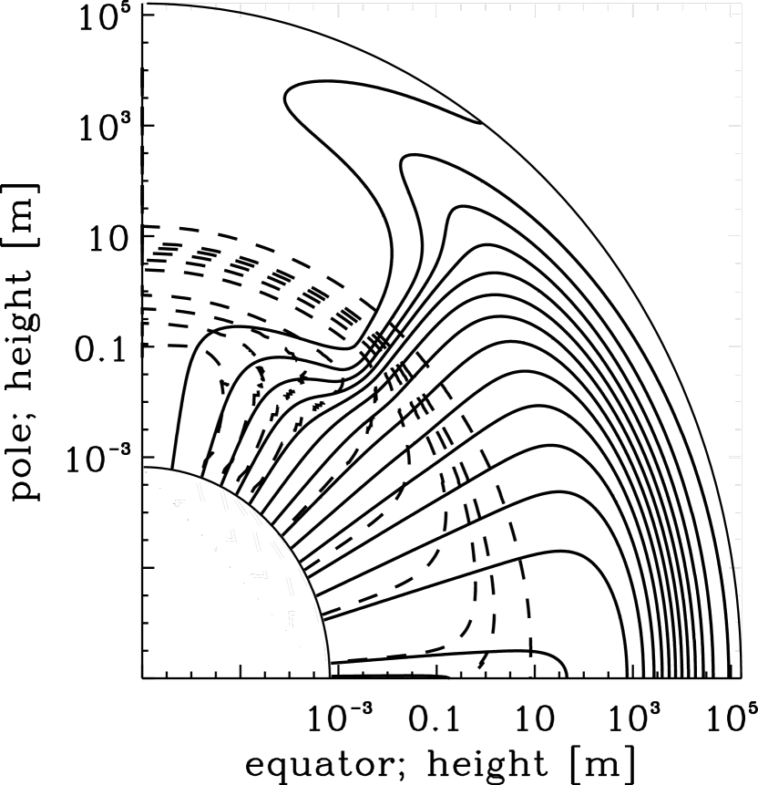
Figure 1: Equilibrium magnetic field lines (solid curves) and density contours (dashed curves) for $M_{\rm a}=10^{-5}M_{\odot}$ and $\psi_{\rm a}=0.1\psi_{*}$. Altitude is marked on the axes (log scale). [From Payne & Melatos (2004).]

Figure 2: Normalized ellipticity $\epsilon(t)/\bar{\epsilon}$ for $M_{\rm a}/M_{\rm c}=0.16,0.80,1.6$, with $\bar{\epsilon}=8.0\times 10^{-7},1.2\times 10^{-6},1.3\times 10^{-6}$ respectively for $b=10$. Time is measured in units of the Alfvén crossing time, $\tau_{\rm A}$.

Figure 3: (Top) Fourier transforms of the wave strain polarization amplitudes $h_{+}(f)$ (left) and $h_{\times}(f)$ (right) for $M_{\rm a}/M_{\rm c}=0.16$ (dashed) and $0.8$ (solid), compared with the LIGO I and II noise curves $h_{3/{\rm yr}}$ (see §4) (dotted). The signals for $M_{\rm a}/M_{\rm c}=0.16$ and $0.8$ yield ${\rm SNR}=2.9$ and $4.4$ respectively after $10^{7}$ s. (Bottom). Zoomed-in view after reducing $h_{+,\times}(f_{*})$ and $h_{+,\times}(2f_{*})$ artificially by 90 per cent to bring out the sidebands. ‘S’ and ‘A’ label the signals induced by sound- and Alfvén-wave wobbles respectively. All curves are for $\alpha=\pi/3$, $i=\pi/3$, $\psi_{*}/\psi_{\rm a}=10$, and $d=10$ kpc.

2.2 Global MHD oscillations

The magnetic mountain is hydromagnetically stable, even though the confining magnetic field is heavily distorted. Numerical simulations using ZEUS-3D, a multipurpose, time-dependent, ideal-MHD code for astrophysical fluid dynamics which uses staggered-mesh finite differencing and operator splitting in three dimensions (Stone & Norman, 1992), show that the equilibria from §2.1 are not disrupted by growing Parker or interchange modes over a wide range of accreted mass ($10^{-7}M_{\odot}\lesssim M_{\rm a}\lesssim 10^{-3}M_{\odot}$) and intervals as long as $10^{4}$ Alfvén crossing times (Payne & Melatos, 2005).

The numerical experiments leading to this conclusion are performed by loading the output ($\rho$ and B) of the Grad-Shafranov code described in Payne & Melatos (2004) into ZEUS-3D, with the time-step determined by the Courant condition satisfied by the fast magnetosonic mode. The code was verified (Payne & Melatos, 2005) by reproducing the classical Parker instability of a plane-parallel magnetic field (Mouschovias, 1974) and the analytic profile of a static, spherical, isothermal atmosphere. Coordinates are rescaled in ZEUS-3D to handle the disparate radial ($c_{\rm s}^{2}R_{*}^{2}/GM_{*}$) and latitudinal ($R_{*}$) length scales. The stability is confirmed by plotting the kinetic, gravitational potential, and magnetic energies as functions of time and observing that the total energy decreases back to its equilibrium value monotonically i.e. the Grad-Shafranov equilibria are (local) energy minima. Note that increasing $\rho$ uniformly (e.g. five-fold) does lead to a transient Parker instability (localized near the pole) in which $\lesssim 1\%$ of the magnetic flux in the ‘tutu’ escapes through the outer boundary, leaving the magnetic dipole and mass ellipticity essentially unaffected.

Although the mountain is stable, it does wobble when perturbed, as sound and Alfvén waves propagate through it (Payne & Melatos, 2005). Consequently, the ellipticity $\epsilon$ of the star oscillates about its mean value $\bar{\epsilon}$. The frequency of the oscillation decreases with $M_{\rm a}$, as described below. The mean value $\bar{\epsilon}$ increases with $M_{\rm a}$ up to a critical mass $M_{\rm c}$ and increases with $\psi_{\rm a}/\psi_{*}$, as described in §3.1.

In ideal MHD, there is no dissipation and the oscillations persist for a long time even if undriven, decaying on the Alfvén radiation time-scale (which is much longer than our longest simulation run). In reality, the oscillations are also damped by ohmic dissipation, which is mimicked (imprecisely) by grid-related losses in our work.

To investigate the oscillations quantitatively, we load slightly perturbed versions of the Grad-Shafranov equilibria in §2.1 into ZEUS-3D and calculate $\epsilon$ as a function of time $t$. Figure 2 shows the results of these numerical experiments. Grad-Shafranov equilibria are difficult to compute directly from (2) and (3) for $M_{\rm a}\gtrsim 1.6M_{\rm c}$, because the magnetic topology changes and bubbles form, so instead we employ a bootstrapping algorithm in ZEUS-3D (Payne & Melatos, 2005), whereby mass is added quasistatically through the outer boundary and the magnetic field at the outer boundary is freed to allow the mountain to equilibrate. The experiment is performed for $r_{0}/R_{*}=c_{\rm s}^{2}R_{*}/GM_{*}=2\times 10^{-2}$ (to make it computationally tractable) and is then scaled up to neutron star parameters ($r_{0}/R_{*}=5\times 10^{-5}$) according to $\epsilon\propto(R_{*}/r_{0})^{2}$ and $\tau_{\rm A}\propto R_{*}/r_{0}$, where $\tau_{\rm A}$ is the Alfvén crossing time over the hydrostatic scale height $r_{0}$ (Payne & Melatos, 2005).

The long-period wiggles in Figure 2 represent an Alfvén mode with phase speed $v_{\rm A}\propto M_{\rm a}^{-1/2}$; their period roughly triples from $100\tau_{\rm A}$ for $M_{\rm a}/M_{\rm c}=0.16$ to $300\tau_{\rm A}$ for $M_{\rm a}/M_{\rm c}=1.6$. Superposed is a shorter-period sound mode, whose phase speed $c_{\rm s}$ is fixed for all $M_{\rm a}$. Its amplitude is smaller than the Alfvén mode; it appears in all three curves in Figure 2 as a series of small kinks for $t\lesssim 50\tau_{\rm A}$, and is plainly seen at all $t$ for $M_{\rm a}/M_{\rm c}=0.8$. As $M_{\rm a}$ increases, the amplitude of the Alfvén component at frequency $f_{\rm A}\sim 17(M_{\rm a}/M_{\rm c})^{-1/2}$ Hz is enhanced. By contrast, the sound mode stays fixed at a frequency $f_{\rm S}\sim 0.4$ kHz, while its amplitude peaks at $M_{\rm a}\sim M_{\rm c}$ (Payne & Melatos, 2005).

3 Frequency spectrum of the gravitational radiation

In this section, we predict the frequency spectrum of the gravitational-wave signal emitted by freely oscillating and stochastically perturbed magnetic mountains in the standard orthogonal polarizations.

3.1 Polarization amplitudes

The metric perturbation for a biaxial rotator can be written in the transverse-traceless gauge as $h_{ij}^{\rm TT}=h_{+}\,e_{ij}^{+}\ +\ h_{\times}\,e_{ij}^{\times}$, where $e_{ij}^{+}$ and $e_{ij}^{\times}$ are the basis tensors for the $+$ and $\times$ polarizations and the wave strains $h_{+}$ and $h_{\times}$ are given by (Zimmermann & Szedenits, 1979; Bonazzola & Gourgoulhon, 1996)

$$h_{+} = h_{0}\sin\alpha[\cos\alpha\sin i\cos i\cos(\Omega t)$$ (4)

$$\qquad\qquad-\sin\alpha({1+\cos^{2}i})\cos(2\Omega t)]\,,$$

$$h_{\times} = h_{0}\sin\alpha[\cos\alpha\sin i\sin(\Omega t)$$ (5)

$$\qquad\qquad-2\sin\alpha\cos i\sin(2\Omega t)]\ ,$$

with

$$h_{0}={2G}{I}_{zz}{\epsilon}{\Omega^{2}/dc^{4}}\,.$$ (6)

Here, $\Omega=2\pi f_{*}$ is the stellar angular velocity, $i$ is the angle between the rotation axis $\textbf{e}_{z}$ and the line of sight, $\alpha$ is the angle between $\textbf{e}_{z}$ and the magnetic axis of symmetry, and $d$ is the distance of the source from Earth.

The ellipticity is given by ${\epsilon}=|I_{zz}-I_{yy}|/I_{0}$, where $I_{ij}$ denotes the moment-of-inertia tensor and $I_{0}=\frac{2}{5}M_{*}R_{*}^{2}$. In general, $\epsilon$ is a function of $t$; it oscillates about a mean value $\bar{\epsilon}$, as in Figure 2. Interestingly, the oscillation frequency can approach $\Omega$ for certain values of $M_{\rm a}$ (see §3.2), affecting the detectability of the source and complicating the design of matched filters. The mean ellipticity is given by (Melatos & Payne, 2005)

$$\bar{\epsilon}=\cases{1}.4\times 10^{-6}\ \left(\frac{M_{\rm a}}{10^{-2}M_{\rm c}}\right)\left(\frac{B_{*}}{10^{12}{\rm\,G}}\right)^{2}\quad M_{\rm a}\ll M_{\rm c}\\ \frac{5M_{\rm a}}{2M_{*}}\left(1-\frac{3}{2b}\right)\left(1+\frac{M_{\rm a}b^{2}}{8M_{\rm c}}\right)^{-1}\quad\quad\,\,\,\,M_{\rm a}\gtrsim M_{\rm c}$$ (7)

where $M_{\rm c}=GM_{*}B_{*}^{2}R_{*}^{2}/(8c_{\rm s}^{4})$ is the critical mass beyond which the accreted matter bends the field lines appreciably, $b=\psi_{*}/\psi_{\rm a}$ is the hemispheric to polar flux ratio, and $B_{*}$ is the polar magnetic field strength prior to accretion. For $R_{*}=10^{6}$ cm, $c_{\rm s}=10^{8}$ cm s^-1, and $B_{*}=10^{12}$ G, we find $M_{\rm c}=1.2\times 10^{-4}M_{\odot}$. The maximum ellipticity, $\bar{\epsilon}\rightarrow 20M_{\rm c}/(M_{*}b^{2})\sim 10^{-5}(b/10)^{-2}$ as $M_{\rm a}\rightarrow\infty$, greatly exceeds previous estimates, e.g. $\bar{\epsilon}\sim 10^{-12}$ for an undistorted dipole (Katz, 1989; Bonazzola & Gourgoulhon, 1996), due to the heightened Maxwell stress exerted by the compressed equatorial magnetic belt. Note that $\epsilon(t)$ is computed using ZEUS-3D for $b=3$ (to minimize numerical errors) and scaled to larger $b$ using (7).

3.2 Natural oscillations

We begin by studying the undamped, undriven oscillations of the magnetic mountain when it is “plucked”, e.g. when a perturbation is introduced via numerical errors when the equilibrium is translated from the Grad-Shafranov grid to the ZEUS-3D grid (Payne & Melatos, 2005). We calculate $h_{\times}(t)$ and $h_{+}(t)$ for $f_{*}=0.6$ kHz from (4) and (5) and display the Fourier transforms $h_{\times}(f)$ and $h_{+}(f)$ in Figure 3 for two values of $M_{\rm a}$. The lower two panels provide an enlarged view of the spectrum around the peaks; the amplitudes at $f_{*}$ and $2f_{*}$ are divided by ten to help bring out the sidebands.

In the enlarged panels, we see that the principal carrier frequencies $f=f_{*},\,2f_{*}$ are flanked by two lower frequency peaks arising from the Alfvén mode of the oscillating mountain (the rightmost of which is labelled ‘A’). Also, there is a peak (labelled ‘S’) displaced by $\Delta f\sim 0.4$ kHz from the principal carriers which arises from the sound mode; it is clearly visible for $M_{\rm a}/M_{\rm c}=0.8$ and present, albeit imperceptible without magnification, for $M_{\rm a}/M_{\rm c}=0.16$. Moreover, $\epsilon$ diminishes gradually over many $\tau_{\rm A}$ (e.g. in Figure 2, for $M_{\rm a}/M_{\rm c}=0.16$, $\epsilon$ drifts from $1.02\bar{\epsilon}$ to $0.99\bar{\epsilon}$ over $500\tau_{\rm A}$), causing the peaks at $f=f_{*},\,2f_{*}$ to broaden. As $M_{\rm a}$ increases, this broadening increases; the frequency of the Alfvén component scales as $f_{\rm A}\propto M_{\rm a}^{-1/2}$ and its amplitude increases $\propto M_{\rm a}^{1/2}$ (see §2.2); and the frequency of the sound mode stays fixed at $f_{\rm S}\sim 0.4$ kHz (Payne & Melatos, 2005). Note that these frequencies must be scaled to convert from the numerical model ($r_{0}/R_{*}=2\times 10^{-2}$) to a realistic star ($r_{0}/R_{*}=5\times 10^{-5}$); it takes proportionally longer for the signal to cross the mountain (Payne & Melatos, 2005).

3.3 Stochastically driven oscillations

We now study the response of the mountain to a more complex initial perturbation. In reality, oscillations may be excited stochastically by incoming blobs of accreted matter (Wynn & King, 1995) or starquakes that perturb the magnetic footpoints (Link et al., 1998). To test this, we perturb the Grad-Shafranov equilibrium $\psi_{\rm GS}$ with a truncated series of spatial modes such that

$$\psi=\psi_{\rm GS}\{1+\Sigma_{n}\delta_{n}\sin[m\pi(r-R_{*})/(r_{\rm max}-R_{*})]\sin(m\theta)\}$$ (8)

at $t=0$, with mode amplitudes scaling according to a power law $\delta_{n}=0.25m^{-1}$, $m=2n+1$, $0\leq n\leq 3$, as one might expect for a noisy process. We place the outer grid boundary at $r_{\rm max}=R_{*}+10r_{0}$. Figure 4 compares the resulting spectrum to that of the free oscillations in §3.2 for $M_{\rm a}/M_{\rm c}=0.8$. The stochastic oscillations increase the overall signal strength at and away from the carrier frequencies $f_{*}$ and $2f_{*}$. The emitted power also spreads further in frequency, with the full-width half-maximum of the principal carrier peaks measuring $\Delta f\approx 0.25$ kHz (c.f. $\Delta f\approx 0.2$ kHz in Figure 3). However, the overall shape of the spectrum remains unchanged. The Alfvén and sound peaks are partially washed out by the stochastic noise but remain perceptible upon magnification. The signal remains above the LIGO II noise curves in Figure 4; in fact, its detectability can (surprisingly) be enhanced, as we show below in §4.

Figure 4: (Top) Fourier transforms of the wave strain polarization amplitudes $h_{+}(f)$ (left) and $h_{\times}(f)$ (right) for $M_{\rm a}/M_{\rm c}=0.8$ with stochastic (dashed) and natural (solid), oscillations. compared with the LIGO I and II noise curves $h_{3/{\rm yr}}$ (see §4) (dotted) corresponding to 99% confidence after $10^{7}$ s. (Bottom) Zoomed in view with $h_{+,\times}(f_{*})$ and $h_{+,\times}(2f_{*})$ artificially reduced by 90 per cent to bring out the sidebands. ‘S’ and ‘A’ label the signal induced by sound- and Alfvén-wave wobbles respectively. All curves are for $\alpha=\pi/3$, $i=\pi/3$, $\psi_{*}/\psi_{\rm a}=10$, and $d=10$ kpc.

4 Signal-to-noise ratio

In this section, we investigate how oscillations of the mountain affect the SNR of such sources, and how the SNR varies with $M_{\rm a}$. In doing so, we generalize expressions for the SNR and characteristic wave strain $h_{\rm c}$ in the literature to apply to nonaxisymmetric neutron stars oriented with arbitrary $\alpha$ and $i$.

4.1 Individual versus multiple sources

The signal received at Earth from an individual source can be written as $h(t)=F_{+}(t)h_{+}(t)+F_{\times}(t)h_{\times}(t)$, where $F_{+}$ and $F_{\times}$ are detector beam-pattern functions ($0\leq|F_{+,\times}|\leq 1$) which depend on the sky position of the source as well as $\alpha$ and $i$ (Thorne, 1987). The squared SNR is then (Creighton, 2003)

$$\frac{S^{2}}{N^{2}}=4\int_{0}^{\infty}df\,\frac{|h(f)|^{2}}{S_{h}(f)}\,,$$ (9)

where $S_{h}(f)=|h_{3/{\rm yr}}(f)|^{2}$ is the one-sided spectral density sensitivity function of the detector (Figures 3 and 4), corresponding to the weakest source detectable with 99 per cent confidence in $10^{7}$ s of integration time, if the frequency and phase of the signal at the detector are known in advance (Brady et al., 1998).

A characteristic amplitude $h_{\rm c}$ and frequency $f_{\rm c}$ can also be defined in the context of periodic sources. For an individual source, where we know $\alpha$, $i$, $F_{+}$ and $F_{\times}$ in principle, the definitions take the form

$$f_{\rm c}=\left[\int_{0}^{\infty}df\,\frac{|h(f)|^{2}}{S_{h}(f)}\right]^{-1}\ \left[\int_{0}^{\infty}df\,f\frac{|h(f)|^{2}}{S_{h}(f)}\right]\,,$$ (10)

and

$$h_{\rm c}=\frac{S}{N}[S_{h}(f_{\rm c})]^{1/2}\,.$$ (11)

These definitions are valid not only in the special case of an individual source with $\alpha=\pi/2$ (emission at $2f_{*}$ only) but also more generally for arbitrary $\alpha$ (emission at $f_{*}$ and $2f_{*}$). Using (4), (5), (10) and (11), and assuming for the moment that $\epsilon$ is constant (i.e. the mountain does not oscillate), we obtain

$$f_{\rm c}=f_{*}(\chi A_{1}+2A_{2})/(\chi A_{1}+A_{2})\,,$$ (12)

$$\frac{S}{N}=h_{0}[S_{h}(2f_{*})]^{-1/2}(\chi A_{1}+A_{2})^{1/2}\sin\alpha$$ (13)

with $A_{1}=\cos^{2}\alpha\sin^{2}i(F_{+}\cos i+F_{\times})^{2}$, $A_{2}=\sin^{2}\alpha[F_{+}(1+\cos^{2}i)+2F_{\times}\cos i]^{2}$, $\chi=S_{h}(2f_{*})/S_{h}(f_{*})$, and $\eta=S_{h}(f_{c})/S_{h}(f_{*})$. In the frequency range $0.2\leq f\leq 3$ kHz, the LIGO II noise curve is fitted well by $h_{3/{\rm yr}}(f)=10^{-26}(f/0.6{\rm kHz})$ Hz^-1/2 (Brady et al., 1998), implying $\chi=4$. As an example, for ($\alpha,i)=(\pi/3,\pi/3)$, we obtain $f_{\rm c}=1.67f_{*}$, $h_{\rm c}=1.22h_{0}$ and $S/N=2.78(f_{*}/0.6{\rm kHz})(\epsilon/10^{-6})(d/10{\rm kpc})^{-1}$. In the absence of specific knowledge of the source position, we take $F_{\times}=F_{+}=1/\sqrt{5}$ (for motivation, see below).

If the sky position and orientation of individual sources are unknown, it is sometimes useful to calculate the orientation- and polarization-averaged amplitude $\bar{h}_{\rm c}$ and frequency $\bar{f}_{\rm c}$. To do this, one cannot assume $\alpha=\pi/2$, as many authors do (Thorne, 1987; Bildsten, 1998; Brady et al., 1998); sources in an ensemble generally emit at $f_{*}$ and $2f_{*}$. Instead, we replace $|h(f)|^{2}$ by $\langle|h(f)|^{2}\rangle$ in (9), (10) and (11), defining the average as $\langle Q\rangle=\int_{0}^{1}\int_{0}^{1}Q\,d(\cos\alpha)\,d(\cos i)$. This definition is not biased towards sources with small $\alpha$; we prefer it to the average $\langle Q\rangle_{2}=\pi^{-1}\int_{0}^{1}\int_{0}^{\pi}Q\,d\alpha\,d(\cos i)$, introduced in Eq. (87) of Jaranowski et al. (1998). Therefore, given an ensemble of neutron stars with mountains which are not oscillating, we take $\langle F_{+}^{2}\rangle=\langle F_{\times}^{2}\rangle=1/5$ and $\langle F_{+}F_{\times}\rangle=0$ [Eq. (110) of Thorne (1987), c.f. Bonazzola & Gourgoulhon (1996); Jaranowski et al. (1998)], average over $\alpha$ and $i$ to get $\langle A_{1}\sin^{2}\alpha\rangle=8/75$ and $\langle A_{2}\sin^{2}\alpha\rangle=128/75$, and hence arrive at $\bar{f}_{\rm c}=1.80f_{*}$, $\bar{h}_{\rm c}=1.31h_{0}$ and $\langle S^{2}/N^{2}\rangle^{1/2}=2.78(f_{*}/0.6{\rm kHz})(\epsilon/10^{-6})(d/10{\rm kpc})^{-1}$. This ensemble-averaged SNR is similar to the non-averaged value for $(\alpha,i)=(\pi/3,\pi/3)$, a coincidence of the particular choice.

Our predicted SNR, averaged rigorously over $\alpha$ and $i$ as above, is $(2/3)^{1/2}$ times smaller than it would be for $\alpha=\pi/2$, because the (real) extra power at $f_{*}$ does not make up for the (artificial) extra power that comes from assuming that all sources are maximal ($\alpha=\pi/2$) emitters. Our value of $\bar{h}_{\rm c}$ is $9/10$ of the value of $h_{\rm c}$ quoted widely in the literature (Thorne, 1987; Bildsten, 1998; Brady et al., 1998). The latter authors, among others, assume $\alpha=\pi/2$ and average over $i$, whereas we average over $\alpha$ and $i$ to account for signals at both $f_{*}$ and $2f_{*}$; they follow Eq. (55) of Thorne (1987), who, in the context of bursting rather than continuous-wave sources, multiplies $h_{\rm c}$ by $(2/3)^{1/2}$ to reflect a statistical preference for sources with directions and polarizations that give larger SNRs (because they can be seen out to greater distances); and they assume $f_{\rm c}=2f_{*}$ instead of $f_{\rm c}=9f_{*}/5$ as required by (10).

4.2 Oscillations versus static mountain

We now compare a star with an oscillating mountain against a star whose mountain is in equilibrium. We compute (10) and (11) directly from $\epsilon(t)$ as generated by ZEUS-3D (see §2 and 3.1), i.e. without assuming that $h_{+}(f)$ and $h_{\times}(f)$ are pure $\delta$ functions at $f=f_{*},\,2f_{*}$.

Table 1 lists the SNR and associated characteristic quantities for three $M_{\rm a}$ values (and $b=10$) for both the static and oscillating mountains. The case of a particular $\alpha$ and $i$ ($\alpha=i=\pi/3$) is shown along with the average over $\alpha$ and $i$ (Thorne, 1987; Bildsten, 1998; Brady et al., 1998). We see that the oscillations increase the SNR by up to $\sim 15$ per cent; the peaks at $f=f_{*},\,2f_{*}$ are the same amplitude as for a static mountain, but additional signal is contained in the sidebands. At least one peak exceeds the LIGO II noise curve in Figure 3 in each polarization.

4.3 Detectability versus $M_{\rm a}$

The SNR increases with $M_{\rm a}$, primarily because $\bar{\epsilon}$ increases. The effect of the oscillations is more complicated: although the Alfvén sidebands increase in amplitude as $M_{\rm a}$ increases, their frequency displacement from $f=f_{*}$ and $f=2f_{*}$ decreases, as discussed in §3.2, so that the extra power is confined in a narrower range of $f$. However, $\epsilon$ and hence the SNR plateau when $M_{\rm a}$ increases above $M_{\rm c}$ (see §3.1). The net result is that increasing $M_{\rm a}$ by a factor of 10 raises the SNR by less than a factor of two. The SNR saturates at $\sim 3.5$ when averaged over $\alpha$ and $i$ (multiple sources), but can reach $\sim 6$ for a particular source whose orientation is favorable. For our parameters, an accreting neutron star typically becomes detectable with LIGO II once it has accreted $M_{\rm a}\gtrsim 0.1M_{\rm c}$. The base of the mountain may be at a depth where the ions are crystallized, but an analysis of the crystallization properties is beyond the scope of this paper.

Table 1: Signal-to-noise ratio

$f_{*}$ [kHz]	$M_{\rm a}/10^{-4}M_{\odot}$	$f_{\rm c}[{\rm kHz}]$	$h_{\rm c}/10^{-25}$	SNR
	Static	$\alpha=\pi/3$	$i=\pi/3$
0.6	$0.16$	1.003	0.83	2.22
0.6	$0.8$	1.003	1.24	3.34
0.6	$1.6$	1.003	1.35	3.61
	Static	$\langle\,\rangle_{\alpha}$	$\langle\,\rangle_{i}\quad\quad$
0.6	$0.16$	1.08	0.89	2.22
0.6	$0.8$	1.08	1.33	3.34
0.6	$1.6$	1.08	1.44	3.61
	Oscillating	$\alpha=\pi/3$	$i=\pi/3$
0.6	$0.16$	1.008	1.40	2.63
0.6	$0.8$	1.003	2.15	4.02
0.6	$1.6$	1.004	2.27	4.25
	Oscillating	$\langle\,\rangle_{\alpha}$	$\langle\,\rangle_{i}\quad\quad$
0.6	$0.16$	1.056	1.40	2.45
0.6	$0.8$	1.048	2.14	3.74
0.6	$1.6$	1.048	2.26	3.95

5 DISCUSSION

A magnetically confined mountain forms at the magnetic poles of an accreting neutron star during the process of magnetic burial. The mountain, which is generally offset from the spin axis, generates gravitational waves at $f_{*}$ and $2f_{*}$. Sidebands in the gravitational-wave spectrum appear around $f_{*}$ and $2f_{*}$ due to global MHD oscillations of the mountain which may be excited by stochastic variations in accretion rate (e.g. disk instability) or magnetic footpoint motions (e.g. starquake). The spectral peaks at $f_{*}$ and $2f_{*}$ are broadened, with full-widths half-maximum $\Delta f\approx 0.2$ kHz. We find that the SNR increases as a result of these oscillations by up to 15 per cent due to additional signal from around the peaks.

Our results suggest that sources such as SAX J1808.4$-$3658 may be detectable by next generation long-baseline interferometers like LIGO II. Note that, for a neutron star accreting matter at the rate $\dot{M}_{\rm a}\approx 10^{-11}M_{\odot}\,{\rm yr}^{-1}$ (like SAX J1808.4$-$3658), it takes only $10^{7}$ yr to reach $S/N>3$. The characteristic wave strain $h_{\rm c}\sim 4\times 10^{-25}$ is also comparable to that invoked by Bildsten (1998) to explain the observed range of $f_{*}$ in low-mass X-ray binaries. An observationally testable scaling between $h_{\rm c}$ and the magnetic dipole moment $|\mu|$ has been predicted (Melatos & Payne, 2005).

The analysis in §3 and §4 applies to a biaxial star whose principal axis of inertia coincides with the magnetic axis of symmetry and is therefore inclined with respect to the angular momentum axis $J$ in general (for $\alpha\neq 0$). Such a star precesses (Cutler & Jones, 2001), a fact neglected in our analysis up to this point in order to maintain consistency with Bonazzola & Gourgoulhon (1996). The latter authors explicitly disregarded precession, arguing that most of the stellar interior is a fluid (crystalline crust $\lesssim 0.02M_{*}$), so that the precession frequency is reduced by $\sim 10^{5}$ relative to a rigid star (Pines & Shaham, 1974). Equations (4) and (5) display this clearly. They are structurally identical to the equations in both Bonazzola & Gourgoulhon (1996) and Zimmermann & Szedenits (1979), but these papers solve different physical problems. In Zimmermann & Szedenits (1979), $\Omega$ differs from the pulsar spin frequency by the body-frame precession frequency, as expected for a precessing, rigid, Newtonian star, whereas in Bonazzola & Gourgoulhon (1996), $\Omega$ exactly equals the pulsar spin frequency, as expected for a (magnetically) distorted (but nonprecessing) fluid star. Moreover, $\theta$ (which replaces $\alpha$) in Zimmermann & Szedenits (1979) is the angle between the angular momentum vector $J$ (fixed in inertial space) and the principal axis of inertia $\textbf{e}_{3}$, whereas $\alpha$ in Bonazzola & Gourgoulhon (1996) is the angle between the rotation axis $\Omega$ and axis of symmetry $\mu$ of the (magnetic) distortion. Both interpretations match on time-scales that are short compared to the free precession time-scale $\tau_{\rm p}\approx(f_{*}\epsilon)^{-1}$, but the quadrupole moments computed in this paper ($\epsilon\sim 10^{-7}$) and invoked by Bildsten (1998) to explain the spin frequencies of low-mass X-ray binaries ($10^{-8}\leq\epsilon\leq 10^{-7}$) predict $\tau_{\rm p}$ of order hours to days. The effect is therefore likely to be observable, unless internal damping proceeds rapidly. Best estimates (Jones & Andersson, 2002) of the dissipation time-scale give $\approx 3.2{\rm\,yr\,}(Q/10^{4})(0.1{\rm kHz}/f_{*})$ $(I_{0}/10^{44}{\rm g\,cm}^{2})$ $(10^{38}{\rm g\,cm}^{2}/I_{\rm d})$, where $I_{\rm d}$ is the piece of the moment of inertia that “follows” $\textbf{e}_{3}$ (not $\Omega$), and $400\lesssim Q\lesssim 10^{4}$ is the quality factor of the internal damping [e.g. from electrons scattering off superfluid vortices (Alpar & Sauls, 1988)].

Table 2: Precession scenarios and associated gravitational wave signals

	biaxial, $\textbf{e}_{3}\|$ $\Omega$	triaxial, $\textbf{e}_{3}\|$ $\Omega$	$\textbf{e}_{3}\nparallel$ $\Omega$
$\textbf{e}_{3}\|$ $\mu$	zero GW	GW at $2f_{*}$	GW near $f_{*}$ and $2f_{*}$
	no precession	no precession	precession
	no pulses	no pulses	pulses
$\textbf{e}_{3}\nparallel$ $\mu$	zero GW	GW at $2f_{*}$	GW near $f_{*}$ and $2f_{*}$
	no precession	no precession	precession
	pulses	pulses	pulses

Some possible precession scenarios are summarized in Table 2. If we attribute persistent X-ray pulsations to magnetic funnelling onto a polar hot spot, or to a magnetically anisotropic atmospheric opacity, then the angle between $\mu$ and $\Omega$ must be large, leading to precession with a large wobble angle, which would presumably be damped on short time-scales unless it is driven (cf. Chandler wobble). Such a pulsar emits gravitational waves at a frequency near $f_{*}$ (offset by the body-frame precession frequency) and $2f_{*}$. However, the relative orientations of $\mu$, $\Omega$, and $\textbf{e}_{3}$ are determined when the crust of the newly born neutron star crystallizes after birth and subsequently by accretion torques. This is discussed in detail by Melatos (2000). If viscous dissipation in the fluid star forces $\Omega$ to align with $\mu$ before crystallization, and if the symmetry axis of the crust when it crystallizes is along $\Omega$, then $\textbf{e}_{3}$ (of the crystalline crust plus the subsequently accreted mountain), $\mu$, and $\Omega$ are all parallel and there is no precession (nor, indeed, pulsation). But if the crust crystallizes before $\Omega$ has time to align with $\mu$, then $\textbf{e}_{3}$ and $\Omega$ are not necessarily aligned (depending on the relative size of the crystalline and pre-accretion magnetic deformation) and the star does precess. Moreover, this conclusion does not change when a mountain is subsequently accreted along $\mu$; the new $\textbf{e}_{3}$ (nearly, but not exactly, parallel to $\mu$) is still misaligned with $\Omega$ in general. Gravitational waves are emitted at $f_{*}$ and $2f_{*}$. Of course, internal dissipation after crystallization (and, indeed, during accretion) may force $\Omega$ to align with $\textbf{e}_{3}$ (cf. Earth).^, If this occurs, the precession stops and the gravitational wave signal at $f_{*}$ disappears. The smaller signal at $2f_{*}$ persists if the star is triaxial (almost certainly true for any realistic magnetic mountain, even though we do not calculate the triaxiality explicitly in this paper) but disappears if the star is biaxial (which is unlikely). To compute the polarization waveforms with precession included, one may employ the small-wobble-angle expansion for a nearly spherical star derived by Zimmermann (1980) and extended to quadratic order by Van Den Broeck (2005). This calculation lies outside the scope of this paper but constitutes important future work.

Recent coherent, multi-interferometer searches for continuous gravitational waves from nonaxisymmetric pulsars appear to have focused on the signal at $2f_{*}$, to the exclusion of the signal at $f_{*}$. Examples include the S1 science run of the LIGO and GEO 600 detectors, which was used to place an upper limit $\epsilon\leq 2.9\times 10^{-4}$ on the ellipticity of the radio millisecond pulsar J1939$+$2134 (The LIGO Scientific Collaboration: B. Abbott et al., 2004b), and the S2 science run of the three LIGO I detectors (two 4-km arms and one 2-km arm), which was used to place upper limits on $\epsilon$ for 28 isolated pulsars with $f_{*}>25$ Hz (The LIGO Scientific Collaboration: B. Abbott et al., 2004a). Our results indicate that these (time- and frequency-domain) search strategies must be revised to include the signal at $f_{*}$ (if the mountain is static) and even to collect signal within a bandwidth $\Delta f$ centered at $f_{*}$ and $2f_{*}$ (if the mountain oscillates). This remains true under several of the evolutionary scenarios outlined above when precession is included, depending on the (unknown) competitive balance between driving and damping.

The analysis in this paper disregards the fact that LIGO II will be tunable. It is important to redo the SNR calculations with realistic tunable noise curves, to investigate whether the likelihood of detection is maximized by observing near $f_{*}$ or $2f_{*}$. We also do not consider several physical processes that affect magnetic burial, such as sinking of accreted material, Ohmic dissipation, or Hall currents; their importance is estimated roughly by Melatos & Payne (2005). Finally, Doppler shifts due to the Earth’s orbit and rotation (e.g. Bonazzola & Gourgoulhon, 1996) are neglected, as are slow secular drifts in sensitivity during a coherent integration.

References

- Abramowitz & Stegun (1972) Abramowitz, M. & Stegun, I. A. 1972, Handbook of Mathematical Functions (Handbook of Mathematical Functions, New York: Dover, 1972)
- Alpar & Sauls (1988) Alpar, M. A. & Sauls, J. A. 1988, ApJ, 327, 723
- Bildsten (1998) Bildsten, L. 1998, ApJ, 501, L89
- Bonazzola & Gourgoulhon (1996) Bonazzola, S. & Gourgoulhon, E. 1996, A&A, 312, 675
- Brady et al. (1998) Brady, P. R., Creighton, T., Cutler, C., & Schutz, B. F. 1998, Phys. Rev. D, 57, 2101
- Chakrabarty et al. (2003) Chakrabarty, D., Morgan, E. H., Muno, M. P., Galloway, D. K., Wijnands, R., van der Klis, M., & Markwardt, C. B. 2003, Nat, 424, 42
- Cook et al. (1994) Cook, G. B., Shapiro, S. L., & Teukolsky, S. A. 1994, ApJ, 424, 823
- Creighton (2003) Creighton, T. 2003, Classical and Quantum Gravity, 20, 853
- Cutler (2002) Cutler, C. 2002, Phys. Rev. D, 66, 084025
- Cutler & Jones (2001) Cutler, C. & Jones, D. I. 2001, Phys. Rev. D, 63, 024002
- Deshpande & McCulloch (1996) Deshpande, A. A. & McCulloch, P. M. 1996, in ASP Conf. Ser. 105: IAU Colloq. 160: Pulsars: Problems and Progress, 101
- Jaranowski et al. (1998) Jaranowski, P., Królak, A., & Schutz, B. F. 1998, Phys. Rev. D, 58, 063001
- Jones & Andersson (2002) Jones, D. I. & Andersson, N. 2002, MNRAS, 331, 203
- Katz (1989) Katz, J. I. 1989, MNRAS, 239, 751
- Lai (1999) Lai, D. 1999, ApJ, 524, 1030
- Link & Epstein (2001) Link, B. & Epstein, R. I. 2001, ApJ, 556, 392
- Link et al. (1998) Link, B., Franco, L. M., & Epstein, R. I. 1998, ApJ, 508, 838
- Lyne et al. (1988) Lyne, A. G., Pritchard, R. S., & Smith, F. G. 1988, MNRAS, 233, 667
- Melatos (2000) Melatos, A. 2000, MNRAS, 313, 217
- Melatos & Payne (2005) Melatos, A. & Payne, D. J. B. 2005, ApJ, 623, 1044
- Melatos & Phinney (2001) Melatos, A. & Phinney, E. S. 2001, PASA, 18, 421
- Mouschovias (1974) Mouschovias, T. 1974, ApJ, 192, 37
- Payne & Melatos (2004) Payne, D. J. B. & Melatos, A. 2004, MNRAS, 351, 569
- Payne & Melatos (2005) —. 2005, MNRAS, submitted
- Pines & Shaham (1974) Pines, D. & Shaham, J. 1974, Comments on Astrophysics and Space Physics, 6, 37
- Shabanova et al. (2001) Shabanova, T. V., Lyne, A. G., & Urama, J. O. 2001, ApJ, 552, 321
- Shakura et al. (1998) Shakura, N. I., Postnov, K. A., & Prokhorov, M. E. 1998, aa, 331, L37
- Stairs et al. (2000) Stairs, I. H., Lyne, A. G., & Shemar, S. L. 2000, Nat, 406, 484
- Stone & Norman (1992) Stone, J. M. & Norman, M. L. 1992, ApJS, 80, 753
- The LIGO Scientific Collaboration: B. Abbott et al. (2004a) The LIGO Scientific Collaboration: B. Abbott, Kramer, M., & Lyne, A. G. 2004a, ArXiv General Relativity and Quantum Cosmology e-prints
- The LIGO Scientific Collaboration: B. Abbott et al. (2004b) —. 2004b, Phys. Rev. D, 69, 082004
- Thorne (1987) Thorne, K. S. 1987, Gravitational radiation, in Three Hundred Years of Gravitation, edited by W. W. Hawking and W. Israel (Cambridge, MA: Cambridge University Press, 1987), 330–458
- Ushomirsky et al. (2000) Ushomirsky, G., Cutler, C., & Bildsten, L. 2000, MNRAS, 319, 902
- Van Den Broeck (2005) Van Den Broeck, C. 2005, Classical and Quantum Gravity, 22, 1825
- Villarreal & Strohmayer (2004) Villarreal, A. R. & Strohmayer, T. E. 2004, ApJ, 614, L121
- Wijnands et al. (2003) Wijnands, R., van der Klis, M., Homan, J., Chakrabarty, D., Markwardt, C. B., & Morgan, E. H. 2003, Nat, 424, 44
- Wynn & King (1995) Wynn, G. A. & King, A. R. 1995, MNRAS, 275, 9
- Zimmermann (1980) Zimmermann, M. 1980, Phys. Rev. D, 21, 891
- Zimmermann & Szedenits (1979) Zimmermann, M. & Szedenits, E. 1979, Phys. Rev. D, 20, 351