Primordial black hole constraints on non-gaussian inflation models

Abstract

We determine the abundance of primordial black holes (PBHs) formed in the context of non-gaussian models with primordial density perturbations. We consider models with a renormalized $\chi^{2}$ probability distribution function parametrized by the number, $\nu$, of degrees of freedom. We show that if $\nu$ is not too large then the PBH abundance will be altered by several orders of magnitude with respect to the standard gaussian result obtained in the $\nu\to\infty$ limit. We also study the dependence of the spectral index constraints on the nature of the cosmological perturbations for a power-law primordial power spectrum.

I Introduction

Contrary to early beliefs some level of non-gaussianity is expected to be present in all inflationary models. Furthermore, the non-gaussian contribution will in general be scale-dependent (see for example BKMR and references therein). Consequently, a strong non-gaussian component on small-scales may turn out to be consistent with current observations which only allow for small deviations from gaussianity on large cosmological scales Ketal . Topological defect models also produce a scale-dependent non-gaussianity in a natural way ASWA . However, in these models the fluctuations are not primordial but generated actively on increasing larger scales by defect network evolution.

Black holes of various masses are expected to form in the early universe as a result of the collapse of large density perturbations H1 ; ZN . The abundance of PBHs provides useful constraints on the primordial power spectrum over a wide range of small scales (see for example C ; CGL ; GL ; GLMS ; C1 and references there in). Although, the usual calculation assumes gaussian perturbations (see however ref. BP for a discussion of the role of non-gaussian fluctuations in PBH formation), standard constraints will need to be modified when considering non-gaussian models.

The cosmological constraints on the abundance of primordial black holes come either from their contribution to the matter density at the present time or from the cosmological implications which result from their Hawking evaporation H2 . PBHs with mass $M\mathrel{\hbox to0.0pt{\lower 4.0pt\hbox{\hskip 1.0pt$\sim$}\hss}\raise 1.0pt\hbox{$<$}}10^{15}$ will have evaporated by the present epoch but if they have a mass $M\mathrel{\hbox to0.0pt{\lower 4.0pt\hbox{\hskip 1.0pt$\sim$}\hss}\raise 1.0pt\hbox{$>$}}10^{9}$ they will still be present at the nucleossynthesis epoch. Assuming a standard cosmological scenario, the fraction of the universe energy density in PHBs with mass greater than $M$ at the time they form is constrained by observations to be $\mathrel{\hbox to0.0pt{\lower 4.0pt\hbox{\hskip 1.0pt$\sim$}\hss}\raise 1.0pt\hbox{$<$}}10^{-20}$ on any interesting mass scale with more accurate constraints depending on their mass (see for example ref. C1 ).

We will generalize to the non-gaussian case the standard calculation of primordial black hole abundances. This uses the Press-Schechter approach PS in order to estimate the fraction of the energy density in PBHs. An alternative calculation using peaks theory was performed in GLMS using the criterion for black hole formation derived by Shibata and Sasaki SS which refers to the the metric perturbation rather than the density field. However, given the large uncertainties involved the results obtained by the two methods were shown to be consistent.

II The power spectrum

On comoving hypersurfaces there is a simple relation between the density perturbation, $\Delta$, and the curvature perturbation, ${\cal{R_{\rm{c}}}}$ (e.g. LL )

$$\Delta(t,k)=\frac{2(1+w)}{5+3w}\left(\frac{kc}{aH}\right)^{2}{{\cal{R_{\rm{c}}}}}(k)\,.$$ (1)

Here $w=p/\rho$ is the equation of state, $H={\dot{a}}/a$ is the Hubble parameter, $k$ is a comoving wavenumber and $c$ is the speed of light. The power spectra are related by

$${\cal P}_{\Delta}(k)=\frac{4(1+w)^{2}}{(5+3w)^{2}}\left(\frac{kc}{aH}\right)^{4}{\cal P}_{{{\cal{R_{\rm{c}}}}}}(k)\,,$$ (2)

and consequently at horizon crossing

$${\cal P}_{\Delta}(k)=\frac{4(1+w)^{2}}{(5+3w)^{2}}{\cal P}_{{{\cal{R_{\rm{c}}}}}}(k)\,.$$ (3)

If we assume a power-law primordial power spectrum with ${\cal P}_{{\cal{R_{\rm{c}}}}}(k)=A_{{\cal{R_{\rm{c}}}}}(k/k_{0})^{n-1}$ and choose a gaussian window function,

$$W(kR)=\exp{\left(-\frac{k^{2}R^{2}}{2}\right)}\,,$$ (4)

then the variance of the primordial density field smoothed on a scale $R$ at horizon crossing,

$$\sigma_{\Delta}^{2}(R)=\int_{0}^{\infty}W^{2}(kR){\cal P}_{\Delta}(k)\frac{{\rm d}k}{k}\,,$$ (5)

is given by

$$\sigma_{\Delta}^{2}(M)=\frac{2(1+w)^{2}}{(5+3w)^{2}}\frac{A_{{{\cal{R_{\rm{c}}}}}}\Gamma[(n-1)/2]}{(k_{0}R)^{n-1}}\,,$$ (6)

for $n>1$. We note that for $n\leq 1$ the variance of a density field with a power-law primordial power-spectrum diverges due to contributions near $k=0$. However, a small $k$ (large wavelength) cut-off to the power spectrum is expected on physical grounds. Spergel et al. Setal have shown, using the WMAPext+2dFGRS dataset, that $A_{{\cal{R_{\rm{c}}}}}=(0.8\pm 0.1)\times 2.95\times 10^{-9}$ for $k_{0}=0.05{\rm Mpc}^{-1}$. We shall take $w=1/3$ appropriate for the radiation dominated era.

III The PBH abundance

We shall use the Press–Schechter approximation (PS ) to compute the fraction of the energy of the Universe, $f(>M)$, associated with PBHs with masses larger than $M$ at the time they form. The Press–Schechter approximation was originally proposed in the context of initial gaussian density perturbations and was much later generalized to accommodate non-gaussian initial conditions COS .

The mass fraction is assumed to be proportional to the fraction of space in which the linear density contrast, smoothed on the scale $M$, exceeds a given threshold ${\Delta_{\rm{th}}}$:

$$f(>M)=A_{f}\int_{\Delta_{\rm{th}}}^{\infty}P_{R}(\Delta)d\Delta\,.$$ (7)

Here $P_{R}(\Delta)$ is the probability distribution function (PDF) of the linear density field $\Delta$ smoothed on a scale $R$ and $A_{f}$ is assumed to be a constant which can be calculated by requiring that $f(>0)=1$, thus taking into account the accretion of material initially present in underdense regions (note that $A_{f}=2$ in the case of gaussian initial conditions).

This generalization has successfully reproduced the results obtained from $N$-body simulations with non-gaussian initial conditions RB but it has been shown in ref. AV that it does not adequately solve the cloud-in-cloud problem (see also ref. IN ). Although this means that in many models $A_{f}$ is not expected to be exactly constant, it will in general be of order unity. Consequently this small uncertainty will have a negligible impact on our final results and we shall not consider it further in the following analysis (we will use $A_{f}=1$ throughout the paper).

The precise value of the threshold value ${\Delta_{\rm{th}}}$ relevant for the calculation of the PHB abundance is uncertain but we shall use the standard value, ${\Delta_{\rm{th}}}=1/3$, for a radiation dominated universe C . Although there should also be a finite upper limit to the integration in Eq. (7) in practice the upper cut-off is unimportant since $P_{R}(\Delta)$ is usually a rapidly decreasing function of $\Delta$.

In order to implement our calculation one needs to relate the mass $M$ to the comoving smoothing scale $R$. An overdense region in order to collapse must be larger than the Jeans length at maximum expansion which, in the radiation dominated era, is $3^{-1/2}$ times the horizon size. On the other hand, it cannot be larger than the horizon size or otherwise it would form a closed universe separate from our own CH . For simplicity, here we will assume that PBHs will form with roughly the horizon mass. This assumption is only approximately true (in general the mass of primordial black holes is expected to depend on the amplitude, size and shape of the perturbations). It will nevertheless have a small impact on our main results. Hence, when the comoving scale $R=c(Ha)^{-1}$ enters the horizon the horizon mass is

$$M_{H}=\frac{4\pi}{3}\rho(c/H)^{-3}\,,$$ (8)

and primordial black holes with a mass $M=M_{H}$ may form at that time. In the radiation dominated era $\rho\propto g_{\star}^{-1/3}a^{-4}$ where $g_{\star}$ is the number of relativistic degrees of freedom (we approximate the temperature and entropy degrees of freedom as equal). This implies that

$$M_{H}=\frac{c}{2G}\left(\Omega_{\gamma,0}\right)^{1/2}H_{0}R^{2}\left(\frac{2}{g_{\star}}\right)^{1/6}\,.$$ (9)

Taking into account that $\Omega_{\gamma,0}h^{2}=2.5\times 10^{-5}$ it is straightforward to show that

$$\frac{R}{1\,{\rm{Mpc}}}=5\times 10^{-24}\left(\frac{M}{1\,{\rm g}}\right)^{1/2}\left(\frac{g_{\star}}{2}\right)^{1/12}\,.$$ (10)

The number of relativistic degrees of freedom, $g_{\star}$, in the early universe is expected to be of order $100$. However, the smoothing scale $R$ is only weakly dependent on $g_{\star}$ (note that Eq. (10) corrects a minor error in ref. GLMS ).

IV The $\chi^{2}$ model

We consider an initial density field with a chi-squared probability distribution function (PDF) with $\nu$ degrees of freedom, the PDF having been shifted so that its mean is zero (such a PDF becomes gaussian when $\nu\to\infty$). Hence,

$$f(>M)=Q(\nu/2,\Delta_{th}/\sigma_{\Delta}\times{\sqrt{\nu/2}}+\nu/2)\,,$$ (11)

where $Q(a,x)$ with $a>0$ is the incomplete gamma function defined by

$$Q(a,x)\equiv\frac{\Gamma(a,x)}{\Gamma(a)}\,.$$ (12)

Here

$$\Gamma(a,x)\equiv\int_{x}^{\infty}e^{-t}t^{a-1}dt$$ (13)

and $\Gamma(a)=\Gamma(a,0)$. If $\nu\to\infty$ then

$$f(>M)\to\frac{1}{2}{\rm erfc}\left(\frac{\Delta_{th}}{{\sqrt{2}}\sigma_{\Delta}}\right)\,.$$ (14)

We further assume that the shape of the PDF is scale independent, that is $P_{R}(\Delta)\equiv P(R,\Delta/\sigma_{\Delta}(R))/\sigma_{\Delta}(R)$ is always the same function (or equivalently $\nu$ does not depend on $R$). Although this is not expected to be precisely true in realistic models, it may be a good approximation over the range of scales relevant for the determination of PBH abundances.

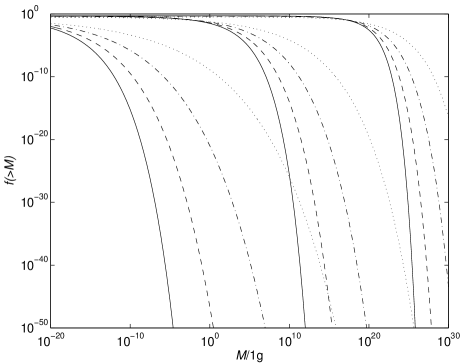
Figure 1: PBH abundance as a function of black hole mass for power-law power spectra with $n=1.2$, $n=1.3$ and $n=1.5$ (sets of curves from left to right respectively) in a $\chi^{2}$ model with $n=\infty$, $n=100$, $n=10$ and $n=1$ degrees of freedom (solid, dashed, dot-dashed and dotted lines respectively).

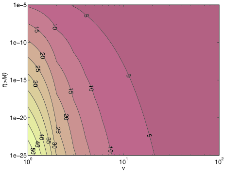
Figure 2: The value of $\alpha$ (defined as the ratio between the amplitudes of the perturbations in a standard gaussian model and in a $\chi^{2}$ model with identical mass functions, $f(>M)$, at a given mass, $M$) as a function of $\nu$ and $f(>M)$. Note that as expected $\alpha$ decreases with increasing $\nu$ (approaching $1$ when $\nu\to\infty$). Also, for a fixed $\nu$ a smaller $f(>M)$ implies a larger $\alpha$.

V Results and discussion

In Fig. 1 we plot the PBH abundance as a function of black hole mass assuming a power-law spectra with $n=1.2$, $n=1.3$ and $n=1.5$ (sets of curves from left to right respectively). The gaussian model is represented by a solid line and the dashed, dot-dashed and dotted lines represent $\chi^{2}$ models with $n=100$, $n=10$ and $n=1$ degrees of freedom respectively. We clearly see that even a small amount of non-gaussianity may have a large impact on the estimated PBH abundance. This shows that an improper use of the standard gaussian assumption may introduce errors on the estimated PBH abundance of many orders of magnitude.

It is useful to determine the impact of non-gaussianity on the spectral index constraint, $n$. We clearly see from Fig. 1 that for $\chi^{2}$ models with a finite numbers of degrees of freedom the constraints are strengthened since for the same value of the spectral index the PHB abundance is significantly increased. Still, this will at most shift the spectral index constraint down by about $0.1$ (in the most extreme case with $\nu=1$).

It is also interesting to ask how much larger the amplitude of the perturbations has to be in a standard gaussian model relative to a $\chi^{2}$ model in order for the mass functions $f(>M)$ at a given mass to be the same. An answer to this question is easily obtained by solving the equations

$$\frac{1}{2}{\rm erfc}\left(x\right) = f(>M)\,,$$

$$Q(\nu/2,x\alpha{\sqrt{\nu}}+\nu/2) = f(>M)\,.$$ (15)

with respect to $\alpha$ for a given $\nu$ and $f(>M)$. The results are shown in Fig. 2. As expected we clearly see that if $\nu$ is increased then $\alpha$ decreases (approaching $1$ when $\nu\to\infty$). Also, for a fixed $\nu$ a smaller $f(>M)$ implies a larger $\alpha$ since the differences between gaussian and $\chi^{2}$ probability distribution functions (for $\nu\neq\infty$) become more dramatic as we move deeper into the distribution tail.

In this study we do not compute the PBH for any specific model of inflation. Still, we expect the $\chi^{2}$ class of models we investigate in this paper to be representative of a large family of non-gaussian models which may be realized in the context of specific inflationary scenarios. The simple assumptions made in this paper also have the advantage of allowing for a complete separation between the effect of the power spectrum (which controls the amplitude of density perturbations on the scales relevant for the calculation of PBHs abundances) from the distribution of the phases of the various Fourier modes. Although, it is possible to consider stronger deviations from a gaussian random distribution which would modify the constraints even further, it might be difficult to construct realistic models where such deviations are incorporated in a natural way.

References

- (1) N. Bartolo, E. Komatsu, S. Matarrese and A. Riotto, Phys. Rept. 402, 103 (2004), astro-ph/0406398.
- (2) E. Komatsu et al., Astrophys. J. Supp. 148, 119 (2003), astro-ph/0302203.
- (3) P. P. Avelino, E. P. S. Shellard, J. H. P. Wu and B. Allen, Astrophys. J. 507, L101 (1998), astro-ph/9803120.
- (4) S. W. Hawking, Mon. Not. Roy. Ast. Soc. 152, 75 (1971).
- (5) Ya. B. Zel’dovich, I. D. Novikov, Sov. Astron. A. J 10, 602 (1967).
- (6) B. J. Carr, Astrophys. J. 201, 1 (1975).
- (7) B. J. Carr, J. H. Gilbert, and J. E. Lidsey, Phys. Rev. D 50, 4853 (1994), astro-ph/9405027.
- (8) A. M. Green and A. R. Liddle, Phys. Rev. D 56, 6166 (1997), astro-ph/9704251.
- (9) A. M. Green, A. R. Liddle, K. A. Malik and M. Sasaki, Phys. Rev. D 70, 041502 (2004), astro-ph/0403181.
- (10) B. J. Carr, astro-ph/0504034.
- (11) James S. Bullock, Joel R. Primack, Phys. Rev. D 55, 7423 (1997), astro-ph/9611106.
- (12) S. W. Hawking, Nature 248, 30 (1974).
- (13) W. H. Press and P. Schechter, 1974, Astrophys. J. 187, 452 (1974).
- (14) M. Shibata and M. Sasaki, Phys Rev. D 60, 084002 (1999), gr-qc/9905064.
- (15) A. R. Liddle and D. H. Lyth, Cosmological Inflation and Large-Scale Structure, CUP, Cambridge (2000).
- (16) D. N. Spergel et al., Astrophys. J. Supp. 148, 175 (2003), astro-ph/0302209.
- (17) W. A. Chiu, J. P. Ostriker, M. A. Strauss, Astophys. J. 479, 490 (1998), astro-ph/9708250.
- (18) Robinson J., Baker J. E., Mon. Not. Roy. Ast. Soc. 311, 781 (2000), astro-ph/9905098.
- (19) P. P. Avelino and P. T. P. Viana, 2000, Mon. Not. Roy. Ast. Soc. 314, 354 (2000), astro-ph/9907209.
- (20) K. T. Inoue, M. Nagashima, Astrophys. J. 574, 9 (2002), astro-ph/0110503.
- (21) B. J. Carr and S. W. Hawking, Mon. Not. Roy. Ast. Soc. 168, 399 (1974).