To Understand the UV-optical Excess of RX J1856.5-3754

Abstract

The enigma source, RX J1856.5-3754, is one of the so-called dim thermal neutron stars. Two puzzles of RXJ1856.5-3754 exist: (1) the observational X-ray spectrum is completely featureless; (2) the UV-optical intensity is about seven times larger than that given by the continuation of the blackbody model yielded by the X-ray data. Both the puzzles would not exist anymore if RX J1856.5-3754 is a low mass bare strange quark star, which is in a propeller phase with a low accretion rate. A boundary layer of RX J1856.5-3754 is suggested and modelled, from which the UV-optical emission is radiated. Free-free absorption dominates the opacity of the boundary layer, which results in the opacity to be high in UV-optical but low in X-ray bands. The star’s magnetic field, spin period, as well as the accretion rate are constrained by observations.

1 Introduction

Quarks (and leptons) are fundamental fermions in the standard model of particle physics, the underlying theory of the interaction between which is believed to be quantum chromodynamics (QCD). Quark matter (or quark-gluon plasma) is expected in QCD, but is not uncovered with certainty. While physicists are trying hard to find quark matter by ground-based colliders, astronomers are researching on the existence and/or consequence of quark matter in the sky. Quark (matter) stars may form by supernova explosions, which are suggested to manifest as pulsar-like compact stars. RX J1856.5-3754 (hereafter RX J1856) is one of the ROSAT-discovered so-called dim thermal neutron stars. It was thought to be actually a quark star (Drake, J. et al., 2002; Xu, 2002). But this idea was soon questioned by Walter & Lattimer (2002) if a two-blackbody model is assumed in order to fit the observations by Chandra, EUVE, and HST.

Among the isolated compact objects, RX J1856 is the mostly studied one because it is the brightest. The parallax distance of this source is only $117\pm 12$ pc (Walter & Lattimer, 2002). Its optical counterpart, with V$\sim$26 mag, was found (Walter & Matthews, 1997), but no radio counterpart has been observed. A 505-ks Chandra observation revealed a featureless spectrum which can be well fitted by a blackbody, with apparent radius $R_{\infty}$= 4.4 km and temperature $T_{\infty}$= 63 eV (Burwitz et al., 2003), and no X-ray modulation being found. Ransom et al. (2002) setted an upper limit on the pulsed fraction of $\sim$4.5% (99% confidence) for frequency $\lesssim$ 50 Hz and frequency derivative $-5\times 10^{10}{\rm~{}Hz~{}s^{-1}}\leq f\leq 0{\rm~{}Hz~{}s^{-1}}$, whereas Burwitz et al. (2003) obtained an upper limit of 1.3% (2$\sigma$ confidence) on the pulsed fraction in the frequency range $(10^{-3}-50)$ Hz using XMM-Newton data.

Various efforts have been made to explain the observations in the regime of normal neutron star, such as a two-component blackbody (Trümper et al., 2003), a neutron star with reflective surface (Burwitz et al., 2003), a magnetar with high kick-velocity (Mori & Ruderman, 2003), a naked neutron star (Turolla et al., 2004), and a surface with strong magnetic field (van Adelsberg et al., 2005; Pérez-Azorín, Miralles & Pons, 2005). But these models are far away from fitting the real data with reasonable emissivity. Summarily, several difficulties are in the normal neutron star models. (1) Featureless spectrum could be hard to reproduce by a neutron star with an atmosphere of normal matter. Though strong magnetic field may smear out some spectral features (Lai, 2001), the consequent large spin down luminosity is not observed. (2) Special geometry is needed to explain the no-modulation observation — the pulsar should be aligned or we are situated at the star’s polar direction. (3) A normal neutron star of radius 17 km in the two-component model requires a very low-mass about $0.4M_{\odot}$. The mechanism to form such a normal neutron star is still unknown.

Alternatively, the X-ray observation alone may be understood by assuming RX J1856 to be a low-mass bare strange quark star, and Zhang, Xu & Zhang (2004) fitted well the X-ray data with a phenomenological spectral emissivity in a solid quark star model. However, the UV-optical observations revealed a seven times brighter source comparing to that derived from X-ray observation. What’s missed here? To overcome these difficulties, we present a model under low-mass quark star regime. A boundary layer around RX J1856 is proposed in this paper, which is optically thick for UV-optical radiation but is optically thin for X-ray radiation. We can obtain consistency with the observational data, as well as strong constrains on the star’s magnetic field strength and spin period, through this approach.

2 The model

We consider the star to be a bare quark star which would be indicated by the featureless spectrum from the 505-ks Chandra data (Xu, 2002). Since a bare quark star have quark surface instead of atmosphere, it could reproduce a Planck-like spectrum, rather than a spectrum with atomic lines (Xu, 2003). Additionally, the small apparent radius ($R_{\infty}$ = 4.4 km) observed in X-ray band could be another hint. For these reasons, a bare quark star hypothesis might be reasonable. The following discussions are under this hypothesis.

The object, RX J1856, in our model consists of two components: (1) a central bare quark star which radiates X-ray photons; (2) a boundary layer at the magnetic radius $r_{\rm m}$ (Alfvén radius) with a quasi thermal spectrum. There are also two free parameters in our model: (1) $\mu_{\rm m}$, the magnetic moment per unit mass of the quark star; (2) ${\dot{M}}$, the accretion rate. Strong constrains on these two parameters will be given by observations in this model. Accreted matter should be stopped at the magnetosphere and form a boundary layer. According to following calculations, the boundary layer is optically thin for the central X-ray emission but thick for UV-optical emission because the cross section is much smaller for X-ray photons than UV-optical ones. By this model, we can fit the observations in UV-optical and X-ray bands. The details are below.

2.1 The star

For a low-mass quark star, the internal density is almost homogenous (Alcock et al., 1986). The star’s mass and density can be well approximated as

$$M\simeq{\frac{4}{3}}\pi R^{3}\rho~{}~{}{\rm and}~{}~{}\rho\simeq 4{\bar{B}},$$ (1)

respectively, where the bag constant is suggested to be ${\bar{B}}=(60\sim 100)~{}{\rm MeV~{}fm^{-3}}=1.07\sim 1.96\times 10^{14}~{}{\rm g~{}cm^{-3}}.$ A median bag constant, ${\bar{B}}=1.5\times 10^{14}~{}{\rm g~{}cm^{-3}}$, $R_{\infty}$= 4.4 km and $T_{\infty}$= 63 eV are adopted in this paper. Considering general relativistic effects ($R_{\infty}=R/(1-R_{\rm g}/R)^{1/2}$), we have $R$ = 4.3 km, $M=0.097M_{\odot}$, and $R_{\rm g}=2GM/c^{2}=$ 0.29 km. Since $M$ is much less than $1M_{\odot}$, the general relativistic effects are rather small. The magnetic moment $\mu$ of the star could be expressed as (Xu, 2005)

$$\mu=\frac{1}{2}BR^{3}=M\mu_{\rm m}.$$ (2)

This is a relatively free parameter because it spans a large range, $(10^{-4}\sim 10^{-6})~{}{\rm G~{}cm^{3}~{}g^{-1}}$ (Xu, 2005). We use $\mu_{\rm m}$ as a free parameter which will be constrained strongly.

2.2 The boundary layer

Since we have never observed any accretion powers, such as strong X-ray emission and X-ray burst, the accretion rate of the star should be very low. Hence we consider ADAF (advection dominated accretion flow) model for the accretion (e.g., Narayan et al., 1998), which means ${\dot{M}}<\sim 0.01{\dot{M}}_{\rm Edd}$, where ${\dot{M}}_{\rm Edd}$ is Eddington accretion rate of RX J1856,

$${\dot{M}}_{\rm Edd} = 4\pi m_{\rm p}cR/\sigma_{\rm T}\simeq 4.2\times 10^{17}~{}{\rm g~{}s^{-1}},$$ (3)

with $m_{\rm p}$ the proton mass and $\sigma_{\rm T}$ the Thomson cross section. The star should be in a propeller phase, and most of the accretion matter can not be accreted onto the the star’s surface (otherwise the accretion induced X-ray luminosity will be much higher than that we observed).

By the accretion flow, a quasi spherical layer may form at the magnetospheric radius,

$$r_{\rm m}\simeq({{B^{2}R^{6}}\over{{\dot{M}}\sqrt{2GM}}})^{2/7},$$ (4)

which is derived by equaling kinematic energy density of free-fall matter to magnetic energy density. At the magnetospheric radius, $r_{\rm m}$, accreted matter will decelerate and pile up to form a boundary layer. The density at the boundary layer should be high enough to make it an optically thick region. The emission spectrum could then be blackbody-like.

2.3 Constrain from temperature

The UV-optical observation of RX J1856 is in the Rayleigh-Jeans tail of the radiation from the boundary layer. The brightness of a back body for $h\nu\ll kT$ is $B_{\nu}\simeq{2k}\nu^{2}T_{r_{\rm m}}/c^{2}$ , where $k$ is Boltzman constant. The observed flux per unit frequency should then be

$$F_{\nu}=\pi B_{\nu}r_{\rm m}^{2}/d^{2}\simeq 2\pi k{{\nu^{2}}\over{c^{2}}}{{1}\over{d^{2}}}T_{r_{\rm m}}r_{\rm m}^{2},$$ (5)

where $d$ is the the star’s distance to the earth. Observationally, one has

$$T_{r_{\rm m}}r_{\rm m}^{2}={\rm const.=9.5\times 10^{3}~{}eV~{}km}^{2}.$$ (6)

In order to be consistent with observation, the boundary layer’s temperature should be neither too high (not to affect the X-ray spectrum) nor too low (to keep the Rayleigh-Jeans slope), i.e. (Burwitz et al., 2003),

$$4~{}{\rm eV}<T_{r_{\rm m}}<33~{}{\rm eV}.$$ (7)

From Eqs.(2), (4), (6), and (7), one comes to

$$17~{}{\rm km}<({{4M^{2}\mu_{\rm m}^{2}}\over{{\dot{M}}\sqrt{2GM}}})^{2/7}<49~{}{\rm km},$$ (8)

where only $\mu_{\rm m}$ and ${\dot{M}}$ are free parameters if the star’s radius (and thus the mass through Eq.(1)) is determined observationally. These two inequations of Eq.(8) give two dashed lines in ${\dot{M}}$-$\mu_{\rm m}$ diagram and constrain the allowed region to a small belt (see Fig. 1).

2.4 Constrain from optical depth

To reproduce the observed spectrum in UV-optical bands, the boundary layer should be optically thick. We assume that the accreted matter’s radial velocity decreases from free fall velocity $v_{\rm ff}$ to zero at the boundary layer. From mass continuity $\rho v={{{\dot{M}}}/{4\pi r_{\rm m}^{2}}},$ the density $\rho$ should increase inward. The magnetic pressure at radius $r$ is $\mathcal{P}(r)={B(r)^{2}/(8\pi)}=\mu^{2}/(2\pi r^{6}).$ Let’s Consider a cubic mass with border $a$ and density $\rho$ near the boundary layer of the mass flow. The cube would feel a force by the magnetic field

$$F\sim{{\partial\mathcal{P}}\over{\partial r}}a^{3}.$$ (9)

The pressure gradient ${\partial\mathcal{P}}/{\partial r}\propto r_{\rm m}^{-7}$ is proximately a constant if the the layer is thin. With the conservation of radial momentum, $-F{\rm d}t={\rm d}(mv)$, and the definition of differential displacement, ${\rm d}x=-v{\rm d}t$, we have $F{\rm d}x\sim mv{\rm d}v\sim a^{3}\rho v{\rm d}v$. One could then estimate the $x$-value of the layer ($x\simeq 0$ at the bottom where $v\simeq 0$ and $\rho=\rho_{\rm max}$) to be,

$$x\simeq v{{{\dot{M}}}\over{4\pi r_{\rm m}^{2}}}/{{\partial\mathcal{P}}\over{\partial r}}\propto v.$$ (10)

We obtain thus $\rho\propto{1/x}$ since $\rho v$ is a constant. It would not be easy to estimate $\rho_{\rm max}$ since the coupling between the accretion disk and the star’s magnetosphere is difficult to model. We have thus another free parameter, $\rho_{\rm max}$, in our calculations. Note that $v$ is the radial velocity. The total velocity does not decrease so much because the velocity changes direction and most of the accreted matter will be propelled out.

At temperature being higher than 4 eV, one can calculate from Saha equation that nearly all hydrogen atoms is ionized. The opacity is produced mainly by Thomson scattering, bond-free and free-free absorptions. In the following, we show that free-free absorption dominates.

The Thomson cross section $\sigma_{\rm T}$ is a constant, and the optical depth is very small if only Thomson scattering is considered. Free-free absorption is sensitive to density, so it is dominated in the high density region and may result in an optically thick boundary layer. Since free-free absorption coefficient (Rybicki & Lightman, 1979, p. 162)

$$\kappa_{\rm ff}=3.7\times 10^{8}T^{-1/2}Z^{2}n_{\rm e}n_{\rm i}\nu^{-3}(1-\exp(-\frac{h\nu}{kT})){\bar{g}}_{\rm ff},$$ (11)

where $n_{\rm e}$ and $n_{\rm i}$ are electron and ion number density, $Z\sim 1$ is ion charge and ${\bar{g}}_{\rm ff}\sim 1$ is Gaunt factor, optical depth differs by a factor of $\sim 10^{6}$ between UV-optical and X-ray bands. Therefore it is possible that the boundary layer would be always optically thin for the central X-ray emission. Detail calculations confirm this suggestion (see Fig. 2).

Bond-free and bond-bond absorptions should also be considered because these processes may induce features in the spectrum which are not observed yet. An estimation goes as following. For oxygen, the most abundant element after hydrogen and helium, the typical bond-free cross section $\sim 10^{-19}$ cm² in 0.1–1 keV band (Reilman & Manson, 1979). Taking into account its abundance $\sim 10^{-3}$ (number relative to hydrogen), the effective cross section is $\sigma_{\rm bb-bf}\sim 10^{-22}$ cm². The optical depth induced by these absorptions could be smaller than 1 though $\sigma_{\rm bb-bf}$ is about $\sim 10^{2}$ times that of electrons. The model proposed may then still work.

Figure 1: The magnetic moment per unit mass $\mu_{\rm m}$ (${\rm G~{}cm^{3}~{}g^{-1}}$) vs. the accretion rate ${\rm d}M/{\rm d}t$ (same to ${\dot{M}}$, in units of Eddington accretion rate). The dashed line are constrains from Eq.(8). Lines labelled by different $\tau(10{\rm eV})$, the optical depth of the layer for $h\nu=10$ eV, are drawn via Eq.(11). The dotted line is for $\tau(0.1{\rm keV)}=0.1$ with $h\nu=0.1$ keV, through Eq.(11) too. Lines denoted by $f_{\rm rad}$ are for different radiation efficiencies, from Eq.(13). The allowed parameter space is limited by four lines: the two dashed lines, the dotted line, and the line denoted by $\tau(10{\rm eV})=1$. It is evident that $8\times 10^{-9}\lesssim\mu_{\rm m}({\rm G~{}cm^{3}~{}g^{-1}})\lesssim 8\times 10^{-8}$, $10^{-4}\lesssim f_{\rm rad}\lesssim 10^{-2}$, and an accretion rate $10^{-3}\lesssim{\dot{M}}/{\dot{M}}_{\rm Edd}\lesssim 10^{-2}$ which is consistent with the ADAF assumption.

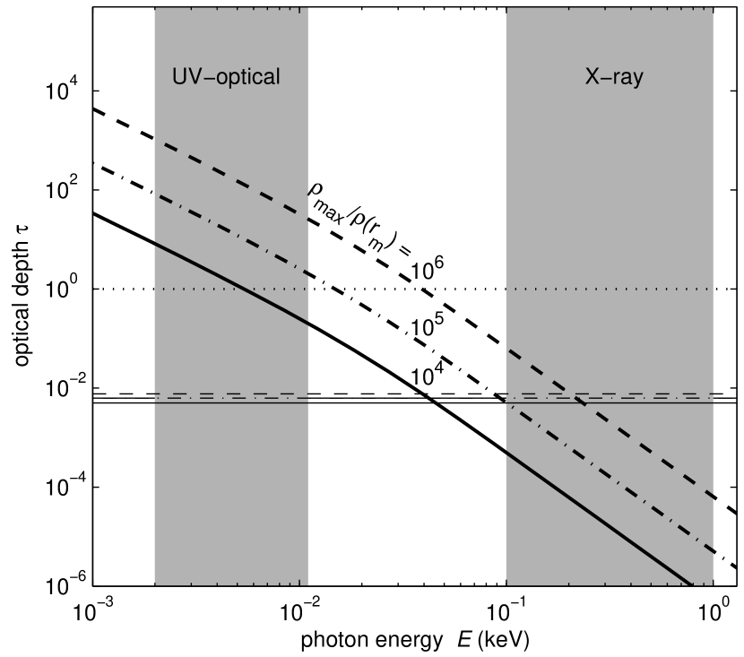
Figure 2: Plot of optical depth $\tau$ vs. photon energy $E$. The bottom density, $\rho_{\rm max}$, is considered as a free parameter. Two hatched regions are for UV-optical and X-ray observations, respectively. The dotted line is for $\tau=1$, beyond which the layer could be optically thick. Thick lines are for free-free absorption, while thin lines for Thomson scattering. Solid, dash-dotted and dashed lines are for different $\rho_{\rm max}$. It is found that the value $\rho_{\rm max}=(10^{5}\sim 10^{6})\rho(r_{\rm m})$ in order to reproduce a boundary layer to be optically thick in UV-optical but thin in X-ray bands, where $\rho(r_{\rm m})={\dot{M}}/(4\pi r_{\rm m}^{2}v_{\rm ff}(r_{\rm m}))$. We choose ${\dot{M}}=10^{-3}{\dot{M}}_{\rm Edd}$ and $\mu_{\rm m}=2\times 10^{-8}~{}{\rm G~{}cm^{3}~{}g^{-1}}$ for indications here.

3 The results

3.1 The radiation efficiency in the layer

Since the star is in a propeller phase, most of the accreted matter will be expelled out finally. In this way only a small part of the accretion energy may be converted to radiation. Here we use $f_{\rm rad}$ to represent the transformation rate. We have then

$${{GM{\dot{M}}}\over{r_{\rm m}}}f_{\rm rad}=\sigma T^{4}\Omega_{\rm BL}r_{\rm m}^{2},$$ (12)

where $\Omega_{\rm BL}$ is the emission angle of the boundary layer which is $4\pi$ if the boundary layer is completely spherical. Since $f_{\rm rad}$ and $\Omega_{\rm BL}$ are degenerate, we adopt simply $\Omega_{\rm BL}=4\pi$ in the following.

Combining with Eqs.(2), (4), (6), and (12), one may obtain the value of a new free parameter $f_{\rm rad}$, the dependence of which on other two free parameters is

$$f_{\rm rad}\simeq 9.24\times 10^{-32}{{{\dot{M}}^{3/7}}\over{\mu_{\rm m}^{20/7}}}.$$ (13)

Different $f_{\rm rad}$ value gives different lines on ${\dot{M}}$-$\mu_{\rm m}$ diagram (see Fig. 1). The allowed range of $f_{\rm rad}$ should be about $10^{-2}\sim 10^{-4}$.

3.2 The star’s spin period and polar magnetic field

A propeller phase requires $r_{\rm co}<r_{\rm m}$, where $r_{\rm co}=(GMP^{2}/(4\pi^{2}))^{1/3}\simeq 6.88\times 10^{7}P^{2/3}$ cm is the corotating radius. We can thus constrain the star’s spin period to be $\lesssim 20$ ms from this requirement. On the $P-{\dot{P}}$ diagram, a death line may simply be represented by an equal voltage line (Zhang, 2003). We therefore constrain $P$ and $\dot{P}$ of RX J1856 via setting the death voltage to be $10^{12}$ V in order to produce approximately the dash-dotted death line for normal pulsars in Fig.3. The death line would be described by

$$\Phi\simeq 6.6\times 10^{12}B_{12}P^{-2}R_{6}^{3}~{}~{}{\rm V}\simeq 10^{12}~{}~{}{\rm V},$$ (14)

where $B_{12}$ is the magnetic field strength in units of $10^{12}$ G and $R_{6}$ is star radius in units of $10^{6}$ cm. The line for RX J1856 is then $0.5B_{12}P^{-2}\simeq 1$. Note that since low-mass quark stars could have small radii, their death line would be different from that of the normal pulsars. A constrain for magnetic polar field (Xu, 2005), $B=32\pi{\bar{B}}\mu_{\rm m}/3$, is obtained so as to make the star radio quiet, $4\times 10^{7}{\rm G}\lesssim B\lesssim 4\times 10^{8}{\rm G}$, from the limit $8\times 10^{-9}\lesssim\mu_{\rm m}({\rm G~{}cm^{3}~{}g^{-1}})\lesssim 8\times 10^{-8}$. We could thus obtain $10^{-22}\lesssim\dot{P}\lesssim 10^{-20}$ in Fig. 3 if a spindown torque by pure magnetodipole radiation is assumed.

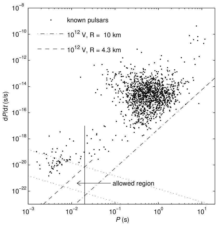
Figure 3: The $P-{\dot{P}}$ diagram and the possible position of RX J1856. RX J1856 should be in the left of the solid vertical line because of $P<20$ ms. It should also be in-between two dotted lines through $4\times 10^{7}\lesssim B{\rm G}\lesssim 4\times 10^{8}{\rm G}$. The dash-dotted and dashed lines are approximately death lines for normal pulsar with radius $R=10$ km and for RX J1856 with $R=4.3$ km, respectively. It is suggested that RX J1856 could be in the triangle (i.e., the “allowed region”) if the star spins down due to pure magnetodipole radiation. No magnetospheric activity exists on the star because of a low potential drop in the open field line region. The pulsar data are from ATNF Pulsar Catalogue (Manchester et al., 2005, http://www.atnf.csiro.au/research/pulsar/psrcat).

4 Conclusions and discussions

We propose that RX J1856.5-3754 is a low-mass quark star, which is in a propeller phase. A boundary layer of RX J1856 is suggested and modelled in order to understand the UV-optical excess observed. In order that the layer could be optically thin in X-ray but thick in UV-optical bands, some constrains for RX J1856 are obtained: the polar magnetic field $4\times 10^{7}{\rm G}\lesssim B\lesssim 4\times 10^{8}{\rm G}$, the spin period $P\lesssim 20$ ms, and an accretion rate $10^{-3}\lesssim{\dot{M}}/{\dot{M}}_{\rm Edd}\lesssim 10^{-2}$, if the the star’s radius and mass are 4.3 km and $\sim 0.1M_{\odot}$, respectively. Additionally, we find that the radiation efficiency of accretion matter in the layer could be between $10^{-2}$ and $10^{-4}$, and that the density at the layer’s bottom is about $10^{5\sim 6}$ times that at the top. No magnetospheric activity exists on the star since it would be under its death line, which could be the reason that neither radio emission nor X-ray modulation is observed from RX J1856. The star could have a weak magnetic field to be similar to that of the millisecond pulsars.

In order to reproduce the UV-optical spectrum, an optically thick layer is considered only, which results naturally a slope of the Rayleigh-Jeans tail. We are still not sure whether the UV-optical spectrum observed could also be understood by an optically thin boundary layer. The difficulty in the later case could be to calculate the emissivity of matter with strong magnetic field. Even in the first case of an optically thick layer, the radiation efficiency is still hard to calculate due to few knowledge of the interaction between charged particles and magnetic field. We obtain a low radiation efficiency, $10^{-4\sim-2}$, in our constrains, which could be reasonable since most of the kinematic energy is take out during a propeller process. The emission from the outer part of the ADAF disk is not taken into account since the luminosity should be very low, with emission in low-energy band.

The bag constant (or effectively, the average density of the star $4{\bar{B}}$) is chosen to be ${\bar{B}}=1.5\times 10^{14}~{}{\rm g~{}cm^{-3}}$ in our calculations. However, the allowed region in $P-{\dot{P}}$ diagram will be larger if $\bar{B}$ is released from 1.07$\times 10^{14}~{}{\rm g~{}cm^{-3}}$ to 1.96$\times 10^{14}~{}{\rm g~{}cm^{-3}}$. The model proposed in this paper would thus be a flexible one.

How to check the model proposed? A direct way might be to find the star’s spin period in radio and/or X-ray data. This model would be rule out if the spin period is much larger than 20ms. Photons in low-energy bands (e.g., infrared or submillimeter emission) would also be radiated from the ADAF disk and the boundary layer. The luminosity of this emission could be high enough if more powerful facilities are offered in the future.

References

- Alcock et al. (1986) Alcock, C., Farhi, E., & Olinto, A. 1986, ApJ, 310, 261
- Burwitz et al. (2003) Burwitz, V., Haberl, F., Neuhäser, R., Predehl, P., Trümper, J., & Zavlin, V. E. 2003, A&A, 399, 1109
- Drake, J. et al. (2002) Drake, J. et al., 2002, ApJ, 572, 996
- Lai (2001) Lai, D. 2001, Rev. Mod. Phys., 73, 629
- Manchester et al. (2005) Manchester, R. N., Hobbs, G. B., Teoh, A. & Hobbs, M. 2005, AJ, 129, 1993
- Mori & Ruderman (2003) Mori, K. & Ruderman, M. A. 2003, ApJ, 592, L75
- Narayan et al. (1998) Narayan, R., Mahadevan, R., & Quataert, E. 1998, in: Theory of Black Hole Accretion Disks, edited by Marek A. Abramowicz, Gunnlaugur Bjornsson, and James E. Pringle. Cambridge University Press, p.148 (astro-ph/9803141)
- Pérez-Azorín, Miralles & Pons (2005) Pérez-Azorín, J. F., Miralles, J. A., & Pons, J. A. 2005, A&A, 433, 275
- Ransom et al. (2002) Ransom, S. M., Gaensler, B. M., & Slane, P. O. 2002, ApJ, 570, L75
- Reilman & Manson (1979) Reilman, R. F., & Manson, S. T. 1979, ApJS, 40, 815
- Rybicki & Lightman (1979) Rybicki, G. B., & Lightman, A. P. 1979, Radiation Process in Astrophysics, (New York: Jhon Wiely & Sons)
- Turolla et al. (2004) Turolla, R, Zane, S., & Drake, J. J. 2004, ApJ, 603, 265
- Trümper et al. (2003) Trümper, J. E., Burwitz, V., Haberl, F., & Zavlin, V. E. 2003, Nuclear Physics B Proceedings Supplements, 132, 560
- van Adelsberg et al. (2005) van Adelsberg, M., Lai, D., Potekhin, A. Y., & Arras, P., 2005, ApJ, 628, 902
- Walter & Lattimer (2002) Walter, F. M., & Lattimer, J. 2002, ApJ, 576, L145
- Walter & Matthews (1997) Walter, F. M., & Matthews, L. D. 1997, Nature 389, 358
- Xu (2002) Xu, R. X. 2002, ApJ, 570, L65
- Xu (2003) Xu, R. X. 2003, ApJ, 596, L59
- Xu (2005) Xu, R. X. 2005, MNRAS, 356, 359
- Zhang, Xu & Zhang (2004) Zhang, X. L., Xu, R. X., & Zhang, S. N. 2004, in: Young neutron stars and their environments, IAU Symp.218, eds. F. Camilo and B. M. Gaensler, p.303
- Zhang (2003) Zhang, B. 2003, Acta Astronomica Sinca (Supplement), 44, 215