Results from the Wide Angle Search for Planets Prototype (WASP0) III: Planet Hunting in the Draco Field

Abstract

The Wide Angle Search for Planets prototype (WASP0) is a wide-field instrument used to search for extra-solar planets via the transit method. Here we present the results of a monitoring program which targeted a 9-degree field in Draco. WASP0 monitored 35000 field stars for two consecutive months. Analysis of the lightcurves resulted in the detection of 11 multi-transit candidates and 3 single-transit candidates, two of which we recommend for further follow-up. Monte-Carlo simulations matching the observing parameters estimate the expected number of transit candidates from this survey. A comparison of the expected number with the number of candidates detected is used to discuss limits on planetary companions to field stars.

1 Introduction

The field of extra-solar planet detection has seen rapid expansion over recent years, both in the number of teams working in the field and in the number of planets detected. This recent expansion has been partly due to the realized potential of the transit method and the ability of relatively cheap instruments as effective tools in searching for transiting extra-solar planets. This was made apparent by the first observation of the transiting planet HD 209458b (Charbonneau et al., 2000; Henry et al., 2000). Since then instruments such as STARE (Brown & Charbonneau, 1999), Vulcan (Borucki et al., 2001), and HAT (Bakos et al., 2002) have greatly contributed to the sky coverage in the search for planetary transits. This has led to other successful detections of transiting planets, such as OGLE-TR-56b (Konacki et al., 2003) and TrES-1 (Alonso et al., 2004). In addition to wide-field searches for transiting planets, a number of narrow-field transit surveys of stellar clusters have been undertaken by several groups (eg., Mochejska et al. (2002); Street et al. (2002)). These narrow-field surveys tend to concentrate on open clusters which are a rich source of young, metal-rich stars.

The reason that the transit method of extra-solar planet detection has become so popular is due to the radial velocity surveys discovering a relatively high number of “hot Jupiters” orbiting solar-type stars. In fact, 0.5%–1% of Sun-like stars in the solar neighbourhood have been found to harbour a Jupiter-mass companion in a 0.05 AU (3–5 day) orbit (Lineweaver & Grether, 2003). It is reasonable to assume that the orbital plane of these short-period planets are randomly oriented, which means that approximately 10% of these planets will transit the face of their parent star as seen by an observer. Thus, the transit method is favoured considering the conclusion that close to 1 in 1000 solar-type stars will produce detectable transits due to an extra-solar planet. Since this transit method clearly favours large planets orbiting their parent stars at small orbital radii, a large sample of stars must be monitored in order to detect statistically meaningful numbers of transiting planets.

The Wide Angle Search for Planets prototype (hereafter WASP0) is an inexpensive wide-field instrument (Kane et al., 2004) developed as a precursor to SuperWASP (Street et al., 2003), a more advanced instrument that has recently been constructed on La Palma, Canary Islands. The primary science goal of both instruments is the detection of transiting extra-solar planets. The first WASP0 observing run was undertaken on La Palma, where observations concentrated on a field in Draco which was regularly monitored for two months. In order to monitor sufficient numbers of stars for successful planetary transit detection, a wide field needs to be combined with reasonably crowded star fields. The Draco field was chosen due to its circum-polar location combined with a relatively high density of field stars. The high sampling rate and duration of monitoring of this field results in a high sensitivity to transiting short-period planets.

We present the results from WASP0 monitoring of the Draco field for transiting extra-solar planets. In sections 2 and 3 we describe the observations and the data reduction methods used to achieve the millimag accuracy required. Section 4 presents results from Monte-Carlo simulations performed which closely match the data from observations of the Draco field. These simulations are used to test the transit detection algorithm described and expected numbers of detectable transiting extra-solar planets are predicted for the data. Section 5 then presents the results of our transit search, including single and multiple-transit candidates. Finally, in section 6 we calculate the resulting limits on planetary companions around field stars and discuss various methods of optimising future transit surveys.

2 Observations

The WASP0 instrument is a wide-field (9-degree) 6.3cm aperture F/2.8 Nikon camera lens, Apogee 10 CCD detector (2K $\times$ 2K chip, 16-arcsec pixels) which was built by Don Pollacco at Queen’s University, Belfast. Calibration frames were used to measure the gain and readout noise of the chip and were found to be 15.44 e^-/ADU and 1.38 ADU respectively. Images from the camera are digitised with 14-bit precision giving a data range of 0–16383 ADUs. The instrument uses a clear filter which has a slightly higher red transmission than blue.

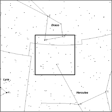
Figure 1: The observed $9^{\circ}\times 9^{\circ}$ field (shown as a square in the center of the figure) which lies in both Draco and Hercules.

WASP0 has had two successful observing runs at two separate sites. The first observing run was undertaken on La Palma, Canary Islands during 2000 June 20 – 2000 August 20. The second observing run took place at Kryoneri, Greece between 2001 October – 2002 May. During the La Palma run, WASP0 was mounted piggy-back on a commercial 8-inch Celestron telescope with a German equatorial mount. These observations concentrated on a field in Draco which was regularly monitored for two months. The location and size of the field is shown in Figure 1. The field center was located at RA. $17^{\mathrm{h}}40^{\mathrm{m}}00^{\mathrm{s}}$ and Dec. 47°55′00″. The observations were interrupted on four occasions when a planetary transit of HD 209458 was predicted. On those nights, a large percentage of time was devoted to observing the HD 209458 field in Pegasus.

Exposure times generally alternated between 20s and 120s to extend the dynamic range so that brighter stars saturated in the longer exposure would be unsaturated in the shorter exposure. However, it was later found that only about 40 additional bright stars were gained by including the 20s frames which at the same time added significant noise to the overall rms of the data. Hence it was decided to only include the 120s frames in the analysis. Further details regarding the observations are described in Kane et al. (2004).

3 Data Reduction

To reduce the large WASP0 dataset, a data reduction reduction pipeline was developed with a high degree of automation. A major challenge for wide-field transit surveys is to produce accurate photometry from the images. This is particularly difficult for wide-fields since there are many spatially-dependent aspects which are normally assumed to be constant across the frame, for example the airmass and heliocentric time correction. These problems have been largely solved by implementing a flux-weighted astrometric fit which uses both the Tycho-2 (Høg et al., 2000) and USNO-B (Monet et al., 2003) catalogues.

Rather than fit the spatially-variable point-spread function (PSF) shape of the stellar images, we used weighted aperture photometry to compute the flux in a circular aperture of tunable radius centred on the predicted positions of all objects in the catalogue. The weights assigned to pixels lying partially outside the aperture are computed using a Fermi-Dirac-like function which are then renormalised to ensure that the effective area of the aperture is $\pi r^{2}$ where $r$ is the aperture radius in pixels. For the WASP0 data, fluxes were computed using apertures of radii 1.5, 2.5, and 3.5 pixels. These fluxes shall be referred to as $F_{1}$, $F_{2}$, and $F_{3}$ respectively.

The most serious issues arise from vignetting and barrel distortion, produced by the camera optics, which alter the position and shape of stellar profiles. In particular, this can result in serious blending effects for stars which neighbour significantly distorted stellar profiles. It has been shown by Brown (2003) and Torres et al. (2004) that blending can have a significant effect on transit searches.

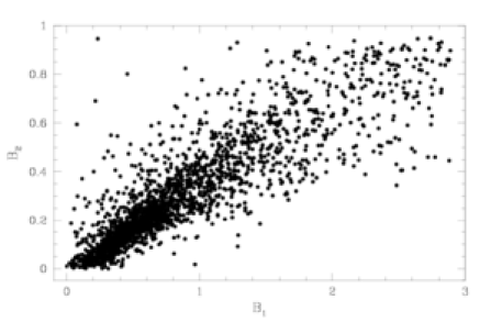
Figure 2: Plot of the two ratios used to distinguish blended from unblended stars. The unblended stars tend to form a tight loucus of stars close to the origin.

In order to identify stars significantly effected by blending, we compute a blending index using the flux measurements from the three different aperture radii. First, we consider the two ratios:

$$B_{1}=\frac{F_{3}-F_{1}}{F_{1}}$$ (1)

and

$$B_{2}=\frac{F_{3}-F_{2}}{F_{2}}$$ (2)

These ratios are plotted in Figure 2 for a typical frame. The purpose of this blend ratio is to provide information about the flux in the core of the stellar profile compared with the flux in the wings. The blend ratio for blended sources tends to increase with a larger aperture size as more flux from neigbouring sources contributes to the total measured flux. The main body of stars in the main locus close to the origin are generally unblended objects whose core-wing ratios are determined by the colour of the star and the chromatic aberration in the lens. The blended stars tend to fall above or below the main locus or fall into a fan which extends beyond the main locus. Direct inspection of the images showed that objects with $(F_{2}-F_{1})/F_{1}$ greater than about the 80th percentile value were invariably found to be either M supergiants or blends, if they lay close to a linear fit to the main locus. Hence, we chose to flag all objects close to the line defined by the main locus with $(F_{2}-F_{1})/F_{1}$ greater than the 80th percentile as likely blends. This method can therefore be used to approximately classify stars as blended or unblended, allowing the blended stars to be excluded from the analysis.

Post-photometry calibrations are applied to remove time-dependent and position-dependent trends from the data. The post-photometry calibration code constructs a theoretical model which is then subtracted from the data leaving residual lightcurves. The residuals are then iteratively fitted to calibrate and remove systematic correlations in the data. Rms accuracy versus magnitude plots are available to evaluate the improvement by applying the model. The de-trended lightcurves are then further analysed for periodic variability including transit signatures. The reduction of the WASP0 data is described in more detail in Kane et al. (2004).

4 Monte-Carlo Simulations

To estimate how many transit events we expect to see in our data, we performed Monte-Carlo simulations which inject transits into fake data and test the capabilities of the transit detection algorithm.

4.1 Simulated Transit Lightcurves

The probability of an observable planetary transit occurring depends upon the inclination of the planet’s orbital plane $i$ satisfying $a\cos i\leq R_{\star}+R_{p}$ where $R_{\star}$ and $R_{p}$ are the radii of the star and planet respectively and $a$ is the semi-major axis of the planet’s orbital radius. The transit probability is then given by $(R_{\star}+R_{p})/a$. As far as the probability is concerned, the size of the planet is of little consequence and depends mostly upon the size of the parent star and orbital radius.

Figure 3: The geometric transit probability (left) and transit duration (right) for planets of Earth and Jupiter radii. The period range has been chosen to match the sensitivity of our survey to multiple transits.

The Draco field was monitored by WASP0 on 29 nights over a period of 35 nights. The Monte-Carlo simulations and transit search has therefore been optimised for an orbital period range of 1–10 days since this is the period range that will most likely yield multiple transiting events for our survey. Shown in Figure 3 are probability and duration plots for Earth and Jupiter radius planets orbiting G5 and M0 main sequence stars. It can be seen from the duration plots that the duration ranges between 2–4 hours for a solar-type star and is a small function of planet radius.

The planetary radius does however matter a great deal for the transit to be detectable, since the fractional transit depth is

$$\frac{\Delta F}{F_{0}}\approx\left(\frac{R_{p}}{R_{\star}}\right)^{2}$$ (3)

where $F_{0}$ is the baseline flux of the star and $\Delta F$ maximum change in flux due to a transit. Shown in Figure 4 are model transits and simulated data for a range of magnitudes and spectral types assuming a single transit by a Jupiter-radius planet and data binning of 10 minutes. The noise model used takes into account detector characteristics as well as photon statistics and takes the form

$$\sigma^{2}=\sigma_{0}^{2}+\frac{(f_{\star}+f_{\mathrm{sky}})\Delta t}{G}$$ (4)

where $\sigma_{0}$ and $G$ are the CCD readout noise (ADU) and gain (e^-/ADU) respectively, $f_{\star}$ and $f_{\mathrm{sky}}$ are the star and sky fluxes respectively, and $\Delta t$ is the exposure time. The plot windows have been normalised to a width of $3R_{\odot}/R_{\star}$, equivalent to the projected path of the planet as it crosses the stellar disk. The depth of the lightcurves is shown to be the same in each case because, although the depth actually varies a great deal, the plots aim to compare the width and shape of the lightcurves and the accuracy of the photometric measurements. Transits of late-type stars are of shorter duration but are considerably deeper and so produce a much higher signal-to-noise (S/N) during the transit. For the WASP0 detector, transits around solar-type stars fainter than 12th magnitude become undetectable although folding data on the orbital period will improve the S/N.

Figure 4: Model transits lightcurves overlaid with simulated data from the WASP0 instrument for a range of spectral types and magnitudes. This assumes the transiting planet is of approximately Jupiter radius.

Figure 5: Properties of stars included in the simulation sample, as derived from the Besançon model. Distributions include the magnitude (top-left), the stellar radii (top-right), the metallicities (bottem-left), and the probability of harbouring a planet (bottom-right).

By applying the noise model shown in equation 4 to the WASP0 detector, simulated lightcurves were generated using the sky values and epochs from the observations. A Besançon model (Robin et al., 2003) tailored to the Draco field observations created a distribution of magnitudes, colours, and metallicities from which stellar parameters were derived. Stellar radii for main sequence stars were calculated directly from the colours provided and giant stars were excluded from the analysis. By utilising the planet-metallicity correlation presented in Fischer & Valenti (2005) which relates stellar metallicity to planetary abundance, the probability of each star harbouring a planet was also computed. Since we are only considering hot Jupiters with a period range of 1–10 days, the resulting probabilities were appropriately weighted by assuming that the periods are approximately uniform in log space (Tabachnik & Tremaine, 2002). Figure 5 shows the histograms of the resulting sample of stars used for the simulations. The stellar population in the Draco field is largely comprised of G dwarf stars with approximately solar metallicity. The power law nature of the Fischer & Valenti (2005) correlation tends to dramatically increase the number of stars with low planet-harbouring probability for a typical metallicity distribution. In particular, stars with metallicities less than $\sim-0.5$ were have essentially zero probability of harbouring a planet, thus resulting in the sharp rise shown in Figure 5.

The existence of a hot Jupiter companion for each star in the sample was randomly determined based on the probability for that star hosting a planet. In cases where a planet was deduced to exist, the planetary radius and the period and inclination of the planetary orbit were randomly generated. Planetary radii were allowed to vary between $0.5R_{J}<R_{p}<1.5R_{J}$ where $R_{J}$ is equivalent to one Jupiter radius. These planetary and stellar radii result in a range of transit depths from 0.1% to 25%. The period was allowed to vary uniformly in log space between 1 and 10 days. In the case of stars which contain a planet with a favourable orbital orientation, the reduction in flux due to a planetary transit was inserted into the data if the star was observed at those epochs. This simulation was run multiple times and a statistical analysis of the expected transit parameters was performed.

Running this simulation many times yielded an average of $\sim 17$ stars with injected transits up to the magnitude limit of 14.5. The distribution of the stars with transits naturally scales with the magnitude distribution shown in Figure 5. The number of cases with transits occurring during observations of the star was found to be $\sim$ 94% including single transits. The number of multiple transits observed was found to be $\sim$ 86%. The probability of observing multiple transits during the course of our observations was calculated for individual periods between 1 and 10 days. This period scan was used to produce the plot shown in Figure 6 which clearly shows the major reduction in probability for periods close to an integer number of days. The figure also shows that almost all transiting planets with periods between 1 and 4 days will produce multiple transits in the data.

Figure 6: Probability of observing at least two transits of a star with injected transits during Draco observations as a function of period.

Although Figure 6 demonstrates the high probability for our data of observing stars with at least two transits, it does not take into account the detectablility of the transit. This restriction is limited by the S/N of the transit and the rms of the associated lightcurve. By running the simulation just once, an entire dataset of lightcurves was generated including injected transits. In order to test the detectability aspect, the lightcurves generated by the simulation were used as input for the transit detection algorithm.

4.2 Transit Detection Algorithm

The ability to efficiently detect the signature of a planetary transit in thousands of lightcurves has been a major challange for the transit survey teams. Automation of transit detection has hence become vigorously studied and several methods have been suggested (eg., DeFaÿ, Deleuil, & Barge (2001); Doyle et al. (2000); Kovács, Zucker, & Mazeh (2002)). Two of the important issues for such methods are the reduction of computational time to a reasonable value and the optimisation of the model to avoid false positive detections. The method used here is a matched-filter algorithm which generates model transit lightcurves for a selected range of transit parameters and then fits them to the stellar lightcurves.

The transit model used for fitting the lightcurves is a truncated cosine approximation with four parameters: period, duration, depth, and the time of transit midpoint. The search first performs a period sweep, optimising the depth and centroid, but holding fixed the duration. The advantage of fixing the duration to a reasonable value and then scanning for multiple transits is that it dramatically reduces the number of false positive detections by avoiding single-dip events. The search is refined by optimising the duration for those stars which are fitted significantly better by the transit model compared with a constant lightcurve model. A transit S/N statistic is calculated for each lightcurve based on the resulting reduced $\chi^{2}$ and $\Delta\chi^{2}$ as follows:

$$S_{W}^{2}=\frac{\Delta\chi^{2}}{\chi_{\mathrm{min}}^{2}/(N-f)}$$ (5)

where $N$ is the number of data points, $f$ is the number of free parameters, and $\Delta\chi^{2}$ is given by

$$\Delta\chi^{2}=\chi_{\mathrm{constant}}^{2}-\chi_{\mathrm{transit}}^{2}.$$

The error bars in the individual lightcurves are rescaled by a factor to force $\chi_{\mathrm{min}}^{2}/(N-f)=1$ for each lightcurve. The $S_{W}$ statistic shown in equation 5 is used consistently throughout the transit detection algorithm, including the first pass in which the transit duration is fixed. By ranking the stars in order of decreasing transit S/N, this becomes an effective method to sift transit candidates from the data.

4.3 Expected Numbers

The simulated lightcurves produced as described in section 4.1 were then analysed using the transit detection algorithm. This exercise is useful for two reasons: to verify the detectability of transits with low S/N and to test the robustness of the detection algorithm.

Around 35000 simulated lightcurves with injected transits were inserted into the transit detection algorithm. A period sweep of 1.1 to 10 days was performed with a fixed duration of 3 hours. This is a fairly computationally expensive exercise for such a large number of stars over such a relatively broad period range. A plot demonstrating the result of this experiment is shown in Figure 7, where the stars with injected transits that transit during observations are shown as 5-pointed stars.

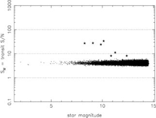
Figure 7: Results of passing the simulated data through the transit detection algorithm. The transit S/N, which measures the “goodness-of-fit” of each lightcurve to a transit model, plotted against magnitude. The stars with injected transits are shown on the diagram as 5-pointed stars.

Figure 7 shows that some of the stars with injected transits have been successfully separated from the bulk of the lightcurves with the majority having a transit S/N $>10$. This also demonstrates the S/N limitations of the data as the number of successful transit extractions decreases significantly as the magnitude limit is approached. In total, $\sim$ 20% of the injected transits were recovered by the detection algorithm. Thus, the expected number of detectable multiple transits in a dataset of 35000 stars is $\sim 47\times 86\%\times 20\%\approx 3$. Additional factors concerning the completeness of the lightcurves and the fraction of blended stars will later be also taken into account.

4.4 Establishing a Candidate Criteria

There are several parameters that can be used to establish a selection criteria for eliminating transit mimics from the list of candidates. These are used consistently as a robust means for producing the final transit candidate list presented in this paper.

Depth: One of the first transit parameters to be yielded from a transit fit is the depth of the transit. As discussed in section 4.1, the expected range of transit depths using typical stellar/planetary radii is 0.2% to 25%. Hence, candidates with depths significantly outside this range can be immediately rejected.

Duration–Period: As shown in Figure 3, there is a relation between transit period and duration that is relatively insensitive to stellar and planetary radii. For example, a transit duration of $\sim 7$ hours would require a period much larger than 10 days, and also a certain amount of luck since the transit probability becomes extremely low outside of 10 days. If the period for a candidate is calculated to be greater than 10 days then the candidate can be rejected.

Transit shape: The shape of the transit lightcurve can be ambiguous in some cases, but a “V-shaped” signature can indicate that the candidate is in fact a grazing eclipsing binary rather than being due to an eclipsing planet.

Colour: Assuming that the star is on the main sequence, the colour combined with the depth allows an approximate calculation of the planetary radii. Clearly this will be more favourable for red stars rather than blue stars.

Multiple transits: Transits candidates for which only one transit is observed are still considered to be candidates. However, since this means that the period is highly uncertain then the candidate is treated with a much higher degree of skeptisicm than candidates for which multiple transits have been observed.

5 Results

This section presents results from the analysis of 29 nights of monitoring the Draco field, including photometric accuracy achieved and transit candidates due to extra-solar planets.

5.1 Photometric Accuracy

Achieving the photometric accuracy necessary to be sensitive to transiting extra-solar planets is one of the many challenges that faces wide-field transit-hunting projects such as WASP0. For WASP0, this has been overcome using the previously described pipeline with very good results, as demonstrated by the rms versus magnitude diagram shown in Figure 8. The instrumental magnitudes are roughly calibrated to $V$ using the Tycho-2 $V$ magnitudes available for the measured stars. The data shown include around 17600 stars at 137 epochs from a single night of WASP0 observations and includes only those stars for which a measurement was obtained at $>90$% of epochs. The upper curve in the diagram indicates the theoretical noise limit for aperture photometry with the 1-$\sigma$ errors being shown by the dashed lines either side. The lower curve indicates the theoretical noise limit for optimal extraction using PSF fitting.

Figure 8: Photometric accuracy versus magnitude diagram from one night of WASP0 observations, showing the rms accuracy in magnitudes in comparison with the theoretical accuracy predicted based on the CCD noise model. The circled line indicates the detection threshold for a Jupiter transiting a solar-type star assuming a distance of 100 pc.

Figure 8 shows that the accuracy achieved for a single night of data is approximately 3 mmag at the bright end. The circled line overlaid on the diagram is for comparison with a predicted transit depth based upon a planet of Jupiter-radius orbiting various main sequence stars. The spectral types range from around solar at the bright end to a late-type (M5) at the faint end. This assumes that the distance to the host star is $d=100\ \mathrm{pc}$. However, since this is a comparison with the per-data-point rms, it is lower than the sensitivity to transit detection which is roughly given by $\mathrm{rms}/\sqrt{P_{t}}$ where $P_{t}$ is the number of data points inside the transit.

5.2 Planetary Transit Search

Figure 9: Results of passing the data through the transit detection algorithm with a period range of between 1 and 10 days with a fixed duration of 3 hours. Each of the plots are plotted against the transit S/N which measures the “goodness-of-fit” of each steller lightcurve to a transit model.

Before subjecting the data to the transit search algorithm, we required that a number of conditions (cuts) be satisfied. The first cut was the removal of blended stars, as discussed in section 3. The effect of this on the number of stars was a reduction of $\sim 25\%$. Finally, only stars for which data were obtained at $>75\%$ of epochs were included, resulting in a dataset of $\sim 14000$ stars.

The large number of stars and epochs required that the data be divided into four magnitude bins in order for it to be managable in terms of memory usage. Since the transit detection algorithm currently uses a grid search rather than an amobea search of parameter space, each magnitude bin took 24–48 hours to perform a period sweep of 1.1 to 10 days with a fixed duration of 3 hours. The plots in Figure 9 show how the algorithm separates the stars with a higher transit S/N from the bulk of the data.

The stars which yielded the highest transit S/N ($S_{W}\ga 10$) were investigated further by performing a duration sweep of 1 to 10 hours. Table 1 lists the best transit candidates that were extracted using this transit detection technique. The candidates have been named WASP0-TR-$N$, where $N$ is the sequence number. Further information on each of the stars, including coordinates, are available via VIZIER (Ochsenbein, Bauer, & Marcout, 2000).

Table 1: List of stars exhibiting transit-like events, where $S_{W}$ is the transit S/N, $P_{t}$ is the number of data points obtained during transit, and $N_{t}$ is the number of transits observed.

candidate	catalogue #	$S_{W}$	$P_{t}$	mag	depth	dur	period	$N_{t}$	colour	$R_{\star}$	$R_{p}$
					(%)	(hours)	(days)		$H-K$	($R_{\odot}$)	($R_{J}$)
WASP0-TR-01	Tycho 3513-00814-1	54.32	25.69	10.51	4.25	9.54	9.27	1	0.069	0.89	1.83
WASP0-TR-02	Tycho 3521-00445-1	46.98	43.79	11.38	10.31	2.33	1.26	6	0.047	1.21	3.89
WASP0-TR-03	USNO 1350-0283522	41.06	14.93	12.46	18.64	3.56	6.35	2	0.065	0.93	4.02
WASP0-TR-04	Tycho 3519-00099-1	31.21	5.33	11.40	17.26	6.87	4.69	1	0.045	1.23	5.11
WASP0-TR-05	Tycho 3519-01199-1	20.04	64.54	12.09	3.61	5.69	2.35	2	0.144	0.64	1.21
WASP0-TR-06	Tycho 3519-01236-1	19.59	7.55	11.48	13.18	8.69	6.03	1	0.058	1.05	3.87
WASP0-TR-07	Tycho 3508-01404-1	9.28	46.99	9.23	0.62	2.95	1.66	?	0.023	1.60	1.26
WASP0-TR-08	USNO 1357-0286817	30.18	28.58	12.69	14.42	4.09	3.82	3	0.073	0.87	3.30
WASP0-TR-09	USNO 1369-0314583	21.17	33.85	13.09	22.75	1.60	1.46	?	0.083	0.82	3.91
WASP0-TR-10	USNO 1357-0286796	17.43	30.10	12.86	8.97	4.09	3.82	2	0.067	0.91	2.72
WASP0-TR-11	USNO 1360-0271503	13.59	49.39	13.05	7.48	1.93	1.15	?	0.089	0.80	2.19
WASP0-TR-12	USNO 1351-0285919	11.42	23.80	12.90	6.53	2.22	2.16	5	0.213	0.49	1.25
WASP0-TR-13	USNO 1333-0303691	32.83	43.67	13.35	43.26	4.29	3.59	4	0.053	1.13	7.43
WASP0-TR-14	USNO 1408-0289086	11.00	6.66	13.54	15.48	1.68	2.09	2	0.079	0.84	3.30

It may at first seem strange to assign a period for which only one transit is observed. However, this means that many periods can be ruled out. These are the periods for which a transit is predicted at a time where data points were taken and show that the predicted transit did not occur. The best-fit period is degenerate, however, because all periods for which the predicted transits occur at times when there are no data points are equally likely. The periodogram for each candidate makes this clear.

The period search used in the transit detection algorithm scans the pre-calculated period grid whilst keeping track of the best period encountered. For a single-transit event, there will be a large number of ties for the best fit period since the $\chi^{2}$ periodogram will be flat at the best-fit value over several period ranges. The first one that occurs in the period grid is retained as the best period. If the search is always conducted from short to long periods, this yields the shortest period that is consistent with the data. This may be considered a reasonably well-defined way of specifying the period for single-transit events.

5.3 Colour-Magnitude Diagram

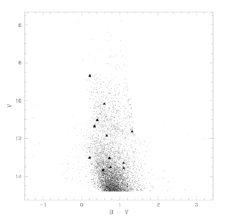
Figure 10: Colour-magnitude diagram for the Draco field with the location of transit candidates shown as triangles.

During the data reduction process, the colours available from the astrometric catalogues for each star are recorded in the output files along with the measured flux. These colours are USNO-B colours or, if available, Tycho-2 colour transformed to the USNO-B colour system. The main difference between these two groups is the precision to which their respective measurements have been obtained, Tycho-2 having a considerably lower rms than the USNO-B measurements. The photometric errors present in either catalogue are sufficiently low to allow the construction of a rough colour-magnitude diagram. Since the Tycho-2 catalogue is 99% complete to $V\sim 11.0$, the source of the colour information in the output files is a reasonable mix of the two catalogues.

Specifically, the USNO-B colours used were second epoch IIIa-J, which approximates as $B$, and second epoch IIIa-F, which approximates as $R$. Kidger (2004) describes a suitable linear transformation from USNO-B filters to the more standard Landolt system. This colour transformation is given by:

$$\mathrm{B:Landolt} = 1.097*\mathrm{USNO(B)}-1.216$$

$$\mathrm{R:Landolt} = 1.031*\mathrm{USNO(R)}-0.417$$

A linear least-squares fit to the colours computed in Bessell (1990) was used to convert from $B-R$ to $B-V$. Using this transformation, we are able to construct an approximate colour-magnitude diagram to investigate the relative location of the transit candidates.

The colour-magnitude diagram shown in Figure 10 appears to show no particular colour trend for the candidates. It is expected that red stars will have deeper transit depths than blue stars. On the other hand, main sequence red stars will also be fainter and therefore more difficult to perform photometry of the necessary accuracy to detect the transit.

5.4 Stellar Radii

Figure 11: The transit depth for planets of radii 0.5, 1.0, and 1.5 $R_{J}$ as a function of colour ($H-K$). The transit candidates are shown on the diagram as 5-pointed stars. Most of the parent stars are G–K and require a planet radius significantly larger than Jupiter’s.

For a reasonable estimate of the stellar radii of the transit candidates, we require colours more accurate than those provided by the Tycho-2 and USNO catalogues. Fortunately, the Two Micron All Sky Survey (2MASS) project provides accurate colours using $J$, $H$, and $K$ filters down to the magnitude limits of the WASP0 data. For the purposes of this study, using $H-K$ for the colour, and hence stellar radii, determination was the best option.

Shown in Figure 11 is a plot of the depth produced by orbiting extra-solar planets of radii 0.5, 1.0, and 1.5 $R_{J}$ as a function of colour ($H-K$). The transit candidates are shown as 5-pointed stars and are predominantly G–K stars. Most of these stars are clustered in the top-left corner of the diagram meaning that the transit depths exhibited by these stars require the transiting planet to have a radius significantly larger than Jupiter’s.

5.5 Transit Candidates

Presented here is a brief discussion for each of the candidates shown in Table 1 and Figures 12–14. There are a number of lightcurves which exhibit transit-like signatures but fail to satisfy the transit selection criteria. These transit mimics are relatively common and must be considered carefully.

Figure 12: Transit candidates 1–5 (top to bottom) from the Draco field.

Figure 13: Transit candidates 6–10 (top to bottom) from the Draco field.

Figure 14: Transit candidates 11–14 (top to bottom) from the Draco field.

WASP0-TR-01: Only one transit was observed and is missing the egress. This creates a degeneracy for the duration measurement (see associatied duration diagram). The colour and transit depth place this candidate slightly outside the region for a 1.5 $R_{J}$ planet (see Figure 11). However, even if the egress had been observed, it is likely that the duration and period don’t match well for this to be considered a real planetary transit.

WASP0-TR-02: This appears to be a likely candidate with a strong S/N and about 6 transits observed. Also, the duration and period are in excellent agreement for a transit candidate. However, the colour of the star shows that a 3.9 $R_{J}$ companion is required to produce the depth fitted, and hence this is unlikely to be a real planetary transit.

WASP0-TR-03: Around 2 transits were observed for this star and the fitted duration and period match very well. The relatively large depth though requires a very late-type star and indeed the colour results in a 4.0 $R_{J}$ companion estimate. Thus this cannot be considered a real planetary transit.

WASP0-TR-04: Although passing initial tests to be selected as a transit candidate, this is unlikely to be real. Only one transit was observed making the period uncertain. The egress was not observed making the fitted duration also uncertain. The colour of the star and the large depth result in a companion radius of 5.0 $R_{J}$.

WASP0-TR-05: About 2 transits have been observed. However, the duration matches poorly with the fitted period. With so few transits observed, there are strong aliases at longer periods. The transit depth and colour indicate a companion radius of 1.2 $R_{J}$. The transit is “V-shaped” which means that this is possibly due to a grazing eclipsing binary rather than a true planetary transit.

WASP0-TR-06: Only one transit was observed for this star casting doubt upon the fitted period. The egress and bottom of the transit were not observed thereby making the fitted duration and depth (which can be treated as a lower limit) also highly uncertain. The colour and depth imply a companion radius of 3.9 $R_{J}$. This is not considered to be a real planetary transit.

WASP0-TR-07: The rms scatter for this star causes the unbinned lightcurve to appear very much like a planetary transit. Once binned (10 minute bins) however, it becomes clear that this is in fact a low amplitude variable star.

WASP0-TR-08: Around 3 transits were observed for this star. The duration and period match closely to what one would expect for a planetary transit. The depth is relatively large and the associated star colour results in an implied companion radius of 3.3 $R_{J}$. Hence this is unlikely to be a real planetary transit.

WASP0-TR-09: Though this was a strong candidate selected by the transit detection algorithm, the binned lightcurve for this star clearly reveals an eclipsing binary system. In particular, this binary appears to be a magnetically active RSCVn binary with a period half that of the fitted period, or around 0.73 days. The colour of the star indicates an early K spectral type. According to the SIMBAD database (Wenger et al., 2000), an x-ray counterpart for this source has been observed using ROSAT, designated 1RXS J174211.8+465442.

WASP0-TR-10: About 2 transits were observed for this candidate and the duration matches well with the fitted period. However, the colour and the depth imply that a 2.7 $R_{J}$ companion, making this unlikely to be due to a planetary transit.

WASP0-TR-11: The duration and period match well for a planetary transit and many transits have been observed. However, binning the lightcurve reveals secondary eclipses. This is in fact an EA/EB type eclipsing binary with a period half that of the fitted period, or around 0.55 days. The colour of the star indicates an early K spectral type.

WASP0-TR-12: This candidate has around 5 transits observed and has a good match between the duration and period. It can be seen that the real period is half that of the fitted period, or around 1.1 days. The colour for this candidate implies a companion radius of 1.25 $R_{J}$ placing it well within planetary candidate range. An alternative explanation for this lightcurve is an EA type eclipsing binary with similar stellar radii producing dips of almost identical depth (such as RX Her). This candidate is worth further follow-up.

WASP0-TR-13: This lightcurve is a good example of a transit mimic for which a strong S/N was calculated by the transit detection algorithm. Although the duration and period are well matched, the transit itself is too deep, the shape of the transit is distinctly “V-shaped”, and there is evidence of a secondary eclipse in the lightcurve, suggesting a grazing eclipsing binary.

WASP0-TR-14: The duration and period are well matched for this candidate for which 2 transits were observed. However, the depth and colour imply a companion radius of 3.3 $R_{J}$. This is therefore unlikely to be a real planetary transit.

6 Discussion

The results of this study shed light on various issues relating to limits on planetary abundances, transit search algorithms, and optimising transit surveys. These will now be discussed in some detail.

6.1 Limits on Planetary Companions around Field Stars

Recent analysis of radial velocity surveys such as Santos et al. (2003) has shown that planets are preferentially found around stars with higher metallicity. This conclusion is further strengthened by the null result of the transit search in 47 Tucanae (Gilliland et al., 2000), an older population with low metallicity. Transit searches in open clusters such as that performed by Bruntt et al. (2003) also produced few candidates suggesting that planetary ejection due to cluster dynamics may play a stronger role in planetary abundances compared to planet formation around stars of low/high metallicity. However, observations of the halo and surrounding field stars of 47 Tucanae by Weldrake et al. (2004) also failed to detect any transiting planets indicating that metallicity is indeed the dominant factor. The field stars surveyed in Draco are predominantly G dwarfs in the solar neighbourhood and therefore of solar metallicity.

Using the model described in section 4.1, the numbers of expected transiting planets with periods in the range 1–10 days is $\sim 17$. Of these, $\sim$ 86% will transit multiple times during the course of the Draco observations. Furthermore, only unblended stars with a high number of epochs (40% of the Draco stars) were searched for transits. Finally, the S/N limits of fainter stars resulted in the transit detection algorithm detecting 20% of the injected transits. Thus, these calculations lead to an expected number of $\sim 1.3$ observed transits in the Draco dataset, or $\sim 1.2$ observed multiple transits. It should of course be noted that the uncertainty in this calculation is expected to be high since even a small change in one of the values will have a significant impact on the result.

Two out of the 14 transit candidates presented in this paper, WASP0-TR-05 and WASP0-TR-12, have the possibility of being due to real transiting planets. However, WASP0-TR-05 has a substantial mis-match between the fitted period and duration and so will not be considered further. This detection rate is in remarkable agreeance with the expected detection rate previously calculated and also with that calculated by Brown (2003). The main contributors to the reduction of our detection rate are blended stars and our photometric precision. If one is able to overcome these two obstacles then one expects, for a similar observing window and magnitude depth, to detect $\sim 15$ multiple transits in the Draco field. Assuming a Poisson distribution, the probability of an event happening $x$ times is given by

$$P(x)=\frac{\mu^{x}e^{-\mu}}{x!}$$ (6)

where $\mu$ is the expected value. If WASP0-TR-12 is a real planetary transit and is the only one in the field ($x=1$), then the probability is calculated to be $4.6\times 10^{-6}$, or significant at the 3.6$\sigma$ level. If all the transit candidates are false and there are none in the field ($x=0$), then the probability is calculated to be $3.1\times 10^{-7}$, or significant at the 3.9$\sigma$ level.

Thus it would be surprising if a more sensitive survey of the Draco field revealed no additional candidates since the metallicity of the Draco stars is similar to that of the stars monitored by the radial velocity surveys. There is no particular direction bias in which radial velocity planets have been discovered since this method generally probes a distance not substantially greater than the solar neighbourhood. A hypothetical lack of planets in the Draco field may suggest that there is indeed a constraint on the metallicity model of planetary abundances in that direction. A lack of planets could also be due to the assumption that planetary periods are approximately uniform in log space which is possibly biased by radial velocity planet discoveries.

6.2 False-Alarm Rate

The false-alarm rate has been a major concern for transit-hunting teams thus far and has vastly increased the necessary CPU and human-effort time required to sift real transit events from the data. Of the 14 transit candidates reported here, almost all appear to be variable stars of some kind. According to the variable star catalogues available via SIMBAD, these stars are all previously unknown variables. The exception to this may be WASP0-TR-09, an RSCVn binary for which an x-ray counterpart is known but has not previously been observed at optical wavelengths. These variable stars produce a high transit S/N in the transit detection algorithm leading to false positives. Assuming that WASP0-TR-12 is a real planetary transit, the false-alarm rate of mimics to planetary transits is 13:1.

A source of false alarms in the Draco dataset was encountered due to the frames in the second half of the night being rotating by 180^∘ relative to frames in the first half of the night. This was due to the use of a German equatorial mount, as described in Kane et al. (2004). The effect of this was to change the shape of PSF profiles and thus cause a magnitude shift in the lightcurves of blended stars. As previously described, most of the blended stars were removed from the dataset prior to analysis. Those blended stars which leaked through into the transit detection algorithm were fitted with an integer day period. Since, as shown in Figure 6, there is a low probability of observing integer day periods, these stars were quickly identified and removed.

The transit detection algorithm could be improved by incorporating many aspects of the transit selection criteria described in this paper. Perhaps the easiest criterion to insert would be an approximate calculation of the period/duration for each candidate and exclude it if there is a significant mis-match. If colour information could be made available, the depth could be translated into planetary radii, thus excluding a major source of mimics. However, transit searches tend to be computationally expensive algorithms and so the challenge is to reduce the false-alarm rate whilst avoiding substantial increases in processing time.

6.3 Follow-up of Transit Candidates

The announcement of various transit candidates have had a significant impact on large telescope subscriptions for radial velocity follow-up. This is particularly true for faint candidates, such as those announced by the OGLE-III project (Udalski et al., 2002). Optimal methods are required for transit mimic elimination to avoid the unnecessary use of large telescope time depending on the nature of the survey. In other words, it is essential to make maximum use of the available photometry before resorting to spectroscopic follow-up.

The first stage of following up transit candidates is to remove transit mimics from the list. The major source of mimics is eclipsing binaries, either grazing eclipsers of $\sim 1\%$ depth or blended eclipsers contributing $\sim 1\%$ of light (Brown, 2003). In most cases, particularly for wide-field surveys such as WASP0 where the stellar profiles are heavily undersampled, straightforward multi-colour observations using a 1.0m telescope can resolve many blended objects. There are also smaller robotic telescopes available, such as Roboscope (Honeycutt, 2000) and Sherlock (Kotredes et al., 2004), which can quickly perform higher angular resolution, multi-colour photometry on transit candidates.

7 Conclusions

This paper describes observations of a field in Draco using the Wide Angle Search for Planets prototype (WASP0). The observations took place over a period of two months from La Palma during which 35000 stars were monitored from this field. The data were reduced using a pipeline which makes use of the Tycho-2 and USNO-B catalogues to provide an astrometric solution for each frame. By considering fluxes measured using multiple apertures, we are able to exclude blended stars from the sample and thus improve our transit search.

By applying the noise model for the instrument and generating a Besançon model for the Draco field, fake data were generated which match the magnitude distribution and epochs of the real data. The metallicity and colours of the Besançon model stars were used to calculate the probability of each star harbouring a planet and the stellar radii. Thus, planetary transits were randomly inserted into the fake dataset. These simulated transits were used to test the transit detection algorithm and to calculate the expected number transits in the entire Draco dataset.

In total, 14000 stars were included in the transit search which yielded 14 transit candidates. Colours extracted from the 2MASS survey were used to estimate the stellar radius and hence the companion radius for each candidate. Of the 14 candidates, 2 were found to pass enough of the selection criteria to be worth further follow-up. The remainder of the candidates are variable stars including one RSCVn binary with an x-ray counterpart. The false-alarm rate from this survey can be reduced in future by incorporating some of the selection criteria into the detection algorithm.

Transit searches have different selection effects from the radial velocity surveys, finding shorter-period planets orbiting lower-mass stars. This will determine how the planet abundance and short-period cutoff seen in radial velocity surveys depend on stellar mass. The two transit candidates identified in this survey are consistent with the expected detection rate considering the constraints of the data and observing window. If however there is indeed a significant lack of transiting planets around Draco field stars then this would be particularly surprising as the field is dominated by G dwarf stars with solar metallicity, and therefore a relatively high probability of harbouring planets. The location of the radial velocity planets do not suggest any such directional bias for planet detection. Future surveys with higher sensitivity, both ground-based and space-based, will resolve this issue.

References

- Alonso et al. (2004) Alonso, R., et al., 2004, ApJ, 613, L153
- Bakos et al. (2002) Bakos, G.Á., Lázár, J., Papp, I., Sári, P., Green, E.M., 2002, PASP, 114, 974
- Bessell (1990) Bessell, M.S., 1990, PASP, 102, 1181
- Borucki et al. (2001) Borucki, W.J., Caldwell, D., Koch, D.G., Webster, L.D., Jenkins, J.M., Ninkov, Z., Showen, R., 2001, PASP, 113, 439
- Brown (2003) Brown, T.M., 2003, ApJ, 593, L125
- Brown & Charbonneau (1999) Brown, T.M., Charbonneau, D., 1999, BAAS, 31, 1534
- Bruntt et al. (2003) Bruntt, H., Grundahl, F., Tingley, B., Frandsen, S., Stetson, P.B., Thomsen, B., 2003, A&A, 410, 323
- Charbonneau et al. (2000) Charbonneau, D., Brown, T.M., Latham, D.W., Mayor, M., 2000, ApJ, 529, L45
- DeFaÿ et al. (2001) DeFaÿ, C., Deleuil, M., Barge, P., 2001, A&A, 365, 330
- Doyle et al. (2000) Doyle, L.R., et al., 2000, ApJ, 535, 338
- Fischer & Valenti (2005) Fischer, D.A., Valenti, J., 2005, ApJ, 622, 1102
- Gilliland et al. (2000) Gilliland, R.L., et al., 2000, ApJ, 545, L47
- Henry et al. (2000) Henry, G.W., Marcy, G.W., Butler, R.P., Vogt, S.S., 2000, ApJ, 529, L41
- Høg et al. (2000) Høg, E., et al., 2000, A&A, 355, L27
- Honeycutt (2000) Honeycutt, R.K., 2000, BAAS, 196, 1903
- Kane et al. (2004) Kane, S.R., Collier Cameron, A., Horne, K., James, D., Lister, T.A., Pollacco, D.L., Street, R.A., Tsapras, Y., 2004, MNRAS, 353, 689
- Kidger (2004) Kidger, M.R., 2004, AJ, submitted
- Konacki et al. (2003) Konacki, M., Torres, G., Jha, S., Sasselov, D., 2003, Nature, 421, 507
- Kotredes et al. (2004) Kotredes, L., Charbonneau, D., O’Donovan, F.T., Looper, D.L., 2004, in AIP Conf. Proc., Vol. 713, The Search for Other Worlds, eds. S.S. Holt & D. Deming, p. 173
- Kovács et al. (2002) Kovács, G., Zucker, S., Mazeh, T., 2002, A&A, 391, 369
- Lineweaver & Grether (2003) Lineweaver, C.H., Grether, D., 2003, ApJ, 598, 1350
- Mochejska et al. (2002) Mochejska, B.J., Stanek, K.Z., Sasselov, D.D., Szentgyorgyi, A.H., 2002, AJ, 123, 3460
- Monet et al. (2003) Monet, D.G., et al., 2003, ApJ, 125, 984
- Ochsenbein et al. (2000) Ochsenbein, F., Bauer, P., Marcout, J., 2000, A&AS, 143, 23
- Robin et al. (2003) Robin, A.C., Reylé, C., Derrière, S., Picaud, S., 2003, A&A, 409, 523
- Santos et al. (2003) Santos, N.C., Israelian, G., Mayor, M., Rebolo, R., Udry, S., 2003, A&A, 398, 363S
- Street et al. (2002) Street, R.A., et al., 2002, MNRAS, 330, 737
- Street et al. (2003) Street, R.A., et al., 2003, ASP Conf. Series, Vol. 294, Scientific Frontiers in Research on Extrasolar Planets, eds. D. Deming & S. Seager, p. 405
- Tabachnik & Tremaine (2002) Tabachnik, S., Tremaine, S., 2002, MNRAS, 335, 151
- Torres et al. (2004) Torres, G., Konacki, M., Sasselov, D.D., Jha, S., 2004, ApJ, 614, 979
- Udalski et al. (2002) Udalski, A., 2002, Acta Astronomica, 52, 1
- Weldrake et al. (2004) Weldrake, D.T.F., Sackett, P.D., Bridges, T.J., Freeman, K.C., 2004, ApJ, in press (astro-ph/0411233)
- Wenger et al. (2000) Wenger, M., et al., 2000, A&AS, 143, 9