Near-Infrared, Kilosecond Variability of the Wisps and Jet
in the Crab Pulsar Wind Nebula

Abstract

We present a time-lapse sequence of 20 near-infrared ($J$- and $K^{\prime}$-band) snapshots of the central $20\arcsec\times 20\arcsec$ of the Crab pulsar wind nebula, taken at subarcsecond resolution with the Hokupa’a/QUIRC adaptive optics camera on the Gemini North Telescope, and sampled at intervals of 10 minutes and 24 hours. It is observed that the equatorial wisps and polar knots in the termination shock of the pulsar wind appear to fluctuate in brightness on kilosecond time-scales. Maximum flux variations of $\pm 24\pm 4$ and $\pm 14\pm 4$ per cent relative to the mean (in $1.2\,{\rm ks}$) are measured for the wisps and knots respectively, with greatest statistical significance in $J$ band where the nebula background is less prominent. The $J$ and $K^{\prime}$ flux densities imply different near-infrared spectra for the nonthermal continuum emission from the wisps and outermost polar knot (‘sprite’), giving $F_{\nu}\propto\nu^{-0.56\pm 0.12}$ and $F_{\nu}\propto\nu^{-0.21\pm 0.13}$ respectively. The data are compared with existing optical and UV photometry and applied to constrain theories of the variability of the wisps (relativistic ion-cyclotron instability) and knots (relativistic fire hose instability).

1 Introduction

Many young pulsars in supernova remnants are embedded in synchrotron nebulae, known as pulsar wind nebulae (PWN), containing relativistic electrons and magnetic flux emitted by the central object. Multiwavelength imaging at subarcsecond resolution reveals that many PWN share a common morphology, consisting of (i) bipolar jets of unequal brightness, directed along the (inferred) pulsar spin axis and terminated by one or more bright knots, and (ii) fibrous arcs, or ‘wisps’, that are cylindrically symmetric about the spin axis, concave or convex with respect to the pulsar, and associated with an X-ray ring and torus. Objects known to display this morphology, likened by some authors to the shape of a crossbow, include the Crab (Hester et al., 1995; Weisskopf et al., 2000; Bietenholz et al., 2001; Hester et al., 2002; Sollerman, 2003), Vela (Pavlov et al., 2001), G320.4$-$1.2 (Gaensler et al., 2002), G54.1$+$0.3 (Lu et al., 2002), 3C58 (Slane et al., 2002), SNR 0540$-$69.3 (Gotthelf & Wang, 2000), and G0.9$+$0.1 (Gaensler et al., 2001), imaged variously by the Chandra X-Ray Observatory (CXO), Hubble Space Telescope (HST), Very Large Telescope (VLT), and Very Large Array (VLA), although there are counter-examples too, e.g. G11.2$-$0.3 (Kaspi et al., 2001). The knots and wisps are interpreted, respectively, as the polar and equatorial zones of the magnetized, collisionless shock terminating the pulsar wind (Gallant & Arons, 1994; Hester et al., 1995; Gaensler et al., 2002; Komissarov & Lyubarsky, 2003; Spitkovsky & Arons, 2004). The brightness asymmetries are ascribed to Doppler boosting. Ideas for explaining jet collimation and the observed jet-torus structure include magnetic hoop stress in the relativistic wind upstream from the shock (Begelman & Li, 1994; Bogovalov, 2001), the anisotropic energy flux in a force-free, monopole wind (Lyubarsky & Eichler, 2001; Lyubarsky, 2002; Komissarov & Lyubarsky, 2003; Del Zanna et al., 2004), magnetic hoop stress or hydromagnetic instabilities in the subsonic, downstream flow (Begelman & Li, 1992; Begelman, 1998; Lyubarsky & Eichler, 2001; Lyubarsky, 2002; Melatos, 2002, 2004), interactions with moving ejecta (Pavlov et al., 2003), and the helical structure of a wave-like, displacement-current-dominated wind (Usov, 1994; Hester et al., 1995; Melatos & Melrose, 1996; Melatos, 1998, 2002).

The subarcsecond features of PWN are highly variable. In the Crab PWN, the optical wisps are seen to change brightness and position in time-lapse HST images every six days, receding from the pulsar concentrically in a wave-like pattern at $\approx 0.5c$, while the optical knots jump around erratically on the same time-scale (Hester et al., 1995, 2002). In contemporaneous CXO images, taken every 22 days, the X-ray ring inside the torus is resolved into more than 20 knots that brighten and fade irregularly, while the X-ray jet transports blobs of material and bow-wave-shaped structures radially outward at $\approx 0.4c$ (Hester et al., 2002; Mori et al., 2002). In time-lapse CXO images of the Vela PWN, Pavlov et al. (2001, 2003) discovered changes of up to 30 per cent over several months in the brightnesses and spectra of the wisps, jet and centrifugal ($0.3$–$0.6c$) knots, coherent bending of the outer jet over 16 days, and changes in knot brightness over just two days. The variability has been ascribed to an ion-cyclotron instability at the shock front (Spitkovsky & Arons, 2004), to a synchrotron cooling instability (Hester et al., 2002), and to a nonlinear Kelvin-Helmholtz instability (Begelman, 1999).

In this paper, we report on the first near-infrared, adaptive-optics observations of the wisps and jet of the Crab PWN. The data offer high angular resolution (optimum $0.\arcsec 19$, average $0.\arcsec 23$ in $K^{\prime}$), high time resolution ($0.6\,{\rm ks}$, resolving the light-crossing and ion-cyclotron time-scales of the narrowest features for the first time), and the first feature-specific continuum color spectra extending from near-infrared to ultraviolet wavelengths. The observations are described in §2, the light curves and spectra of individual features are presented in §3 and §4, and the results are interpreted physically in §5.

2 Observations

The center of the Crab PWN was observed on 2002 February 6, 7, and 8 with the Hokupa’a/QUIRC adaptive optics instrument on the Gemini North Telescope (proposal GN-2002A-Q-16). Hokupa’a is a natural guide star, curvature sensing system with 36 elements, coupled to a near-infrared camera, QUIRC, consisting of a $1024\times 1024$ HgCdTe array with plate scale $0.\arcsec 0200$, dark current $<0.1$ electrons per second, and read-out noise 15–30 electrons. The system is described in detail by Graves et al. (1998). Hokupa’a is capable of locking on to point sources with $R\lesssim 15\,{\rm mag}$ nominally and $R\lesssim 17\,{\rm mag}$ in practice. It is therefore ideal for imaging the Crab PWN, where there are two suitable guide stars within $4\arcsec$ of the center of the nebula (cf. isoplanatic radius $\approx 30\arcsec$): a field star (Star I) at $\alpha(2000)=05^{\rm h}34^{\rm m}32.2^{\rm s}$ and $\delta(2000)=+22^{\circ}00^{\prime}57^{\prime\prime}$, with $R=14.8\pm 0.2\,{\rm mag}$, which we chose to use, and the Crab pulsar, with $R=16.3\,{\rm mag}$ pulse-averaged (Eikenberry et al., 1997). The wavelengths and bandpasses of the QUIRC $J$ and $K^{\prime}$ filters are $1.25\,\mu{\rm m}/0.17\,\mu{\rm m}$ and $2.12\,\mu{\rm m}/0.41\,\mu{\rm m}$ respectively. We achieved resolutions of ${\rm FWHM}=0.\arcsec 19$–$0.\arcsec 30$ in $K^{\prime}$ and ${\rm FWHM}=0.\arcsec 24$–$0.\arcsec 37$ in $J$ in this sequence of observations, where FWHM refers to the full-width half-maximum of the point spread function (PSF). The seeing fluctuated by up to $\pm 0.05\arcsec$ in $K^{\prime}$ and $\pm 0.08\arcsec$ in $J$ over intervals of $0.6\,{\rm ks}$.

We obtained a sequence of $20\times 4\times 0.12\,{\rm ks}$ exposures spaced in a four-point, $3\arcsec$ dither pattern, which were subsequently combined into 20 frames, as follows: $5\times K^{\prime}$ then $3\times J$ (2002 February 6), $3\times J$ then $5\times K^{\prime}$ (2002 February 7), and $4\times K^{\prime}$ (2002 February 8). Conditions were excellent on 2002 February 6. On the following nights, observations were affected by light cloud and wind. Data were gathered without interruption during all three nights, yielding a sampling time of $0.6\,{\rm ks}$ between frames (after read-out), with two brief exceptions: a five-point dither was accidentally performed on 2002 February 6, and two six-point dithers were required on 2002 February 8, when the telescope lost its guiding. All features were observed with good signal-to-noise. In a typical $0.12\,{\rm ks}$ exposure in $K^{\prime}$, we accumulated $\approx 4.9\times 10^{2}$ counts/pixel for the pulsar and guide star, $\approx 4.5\times 10^{1}$ counts/pixel for the brightest extended feature (the sprite; see §3), and $\approx 2.7\times 10^{1}$ counts/pixel for the faintest extended feature (the faint wisp; see §3), after subtracting the nebula background ($2.9$–$5.1\times 10^{3}$ counts/pixel, or $1.1$–$1.9\,{\rm Jy}\,{\rm arcsec^{-2}}$).

We assembled a data reduction pipeline in IRAF to subtract bias, dark, and sky frames and divide by flat fields in the standard way. The three bright point sources in the field were excised from the sky frames with care, to avoid creating false shadows by oversubtraction. After trimming a border 20 pixels wide to remove faulty edge pixels, we median combined each set of four dithered images, rejecting one high, then trimmed a border $3\arcsec$ wide to exclude the region where the four dithered exposures do not overlap.

An important issue with any adaptive optics observation is the degree by which the PSF changes across the field of view. In this work, we can quantify the effect directly by examining the three point sources in the field (the guide star, the pulsar, and a field star $6\arcsec$ south of the pulsar, labeled Star II), which happen to be well separated. We find that the PSF is nearly axisymmetric at the southern field star, elongated in an east-west direction at the pulsar, and elongated in a northeast-southwest direction at the guide star, with minor and major axes in the ratio $\approx 0.8$ (although the isophotes are not strictly elliptical). This essentially precludes accurate photometry of the inner knot, located $0.\arcsec 6$ from the pulsar, for the reasons set forth in §3.2, without prejudicing photometry of large, extended features like the wisps. Another issue is how the PSF varies as a function of time. We do not detect any change in the shape of the PSF at the locations of the three field stars when comparing isophotes from successive exposures by eye. However, there is indirect evidence that slight yet rapid changes do occur; we find that the total flux from the guide star within an aperture of radius $3.1$ ${\rm FWHM}$ fluctuates by $\pm 6$ ($\pm 4$) per cent in $K^{\prime}$ ($J$) over $0.6\,{\rm ks}$ after background subtraction (§3.1), accompanied by fluctuations of $\pm 9$ ($\pm 4$) per cent in the southern field star. These changes feed into the measurement uncertainties calculated in §3 and §4, as the field stars serve as flux calibrators.

3 Kilosecond variability

Figure 1 shows the center of the Crab PWN at $0.\arcsec 19$ resolution (FWHM) in $K^{\prime}$, as it appeared on 2002 February 6. Its crossbow-like morphology is evident. The subarcsecond features in the termination shock of the pulsar wind are cylindrically symmetric about the projected rotation axis and proper motion of the pulsar, determined from HST astrometry (Caraveo & Mignani, 1999).

1. The wisps are interpreted as shock structures in the equatorial plane of the pulsar wind (latitude $\pm 10\deg$), in the neighborhood of the X-ray ring and torus (Hester et al., 1995; Weisskopf et al., 2000; Hester et al., 2002; Mori et al., 2002; Spitkovsky & Arons, 2004; Komissarov & Lyubarsky, 2003; Del Zanna et al., 2004). The faint and bright wisps to the northwest of the pulsar, labeled in Figure 1, mark ion-driven magnetic compressions (at the first and second ion turning points) in the ion-cyclotron model of the shock (Gallant & Arons, 1994; Spitkovsky & Arons, 2004); they are probably analogous to the features labeled 5 and E by Gaensler et al. (2002) in another PWN, G320.4$-$1.2. The position and brightness of these two wisps, several less prominent wisps, and their fibrous substructure are known to change on a time-scale as short as six days in the optical (Hester et al., 2002) and 22 days in X-rays (Hester et al., 2002; Mori et al., 2002).

2. The sprite can be interpreted as a polar shock, lying on the rotation axis (colatitude $\pm 15\deg$) at or near the base of the polar X-ray jet (Weisskopf et al., 2000; Hester et al., 2002; Mori et al., 2002). It can also be interpreted as a mid-latitude arch shock between the polar outflow and equatorial backflow in a pressure-confined, split-monopole nebula, situated at the tangent point of the line of sight (and therefore Doppler boosted) (Komissarov & Lyubarsky, 2003; Del Zanna et al., 2004). Its shape, doughnut-like with a central rod (§3.2), changes irregularly on the same time-scale as the wisps; in CXO images, the sprite appears to be the launching point for blobs and ‘bow waves’ ejected along the X-ray jet (Hester et al., 2002; Mori et al., 2002), although these may also be unstable motions in the vicinity of the mid-latitude arch shock (Komissarov & Lyubarsky, 2003).

3. The inner knot is a barely resolved, flattened (§3.3) structure partly obscured in Figure 1 by the pulsar PSF. It too can be interpreted as a polar feature, lying $\approx 5$ times closer to the pulsar than the sprite. If the sprite marks the polar termination shock, the inner knot sits in the unshocked pulsar wind, and its physical origin is unknown (Hester et al., 1995; Melatos, 1998, 2002). If the sprite is a mid-latitude arch shock, the inner knot originates from a part of the arch shock nearer the base of the polar jet, which is pushed inward (relative to the wisps) because the energy flux in a split-monopole wind is lower at the poles than at the equator (Komissarov & Lyubarsky, 2003).

4. A conical halo is visible at intermediate latitudes, midway between the pulsar and faint wisp in Figure 1, the near-infrared counterpart of an optical feature noted in HST data by Hester et al. (1995). We do not discuss the halo further in this paper, as it is too faint for accurate near-infrared photometry.

In this section, we examine the variability of four features — the bright wisp, faint wisp, sprite, and inner knot — in the near-infrared over time-scales as short as $0.6\,{\rm ks}$, extending previous studies of the Crab PWN with HST (sampling time six days) and CXO (sampling time 22 days) (Hester et al., 2002; Mori et al., 2002). The first (and most challenging) step, subtracting the time-dependent nebula background, is discussed in §3.1. Light curves of the features are presented in §3.2 and §3.3.

3.1 Nebula background

It is difficult to characterize and hence subtract the background in Figure 1, because there is no unique way to disentangle the contributions from the nebula and sky, given that the nebula is ubiquitous, nonuniform, and time-dependent. The surface brightness $I_{\rm o}$ observed in any pixel is the sum of flux from the nebula background ($I_{\rm n}$) and any feature ($I_{\rm f}$) occupying that pixel, with $I_{\rm o}=(I_{\rm n}+I_{\rm f})\eta_{\rm a}+I_{\rm a}$, where $\eta_{\rm a}$ and $I_{\rm a}$ denote the atmospheric absorption coefficient and sky brightness respectively. There are two problems in extracting $I_{\rm f}$ from $I_{\rm o}$. First, there are no pixels empty of both features and nebula, so we cannot measure $I_{\rm a}$ directly. In our analysis, we assume that $\eta_{\rm a}$ and $I_{\rm a}$ are uniform across the field of view, but both parameters vary markedly from exposure to exposure, as quantified below. Second, $I_{\rm n}$ fluctuates stochastically from pixel to pixel, so we cannot estimate $I_{\rm n}$ behind a feature by interpolating $I_{\rm n}$ directly from neighboring, feature-free pixels.

To overcome these problems, we average the observed brightness of all feature-free pixels ($I_{\rm o}^{\prime}$) in the field to obtain $I_{\rm n}\eta_{\rm a}+I_{\rm a}=\langle I_{\rm o}^{\prime}\rangle$ and hence, approximately, $I_{\rm f}\eta_{\rm a}=I_{\rm o}-\langle I_{\rm o}^{\prime}\rangle$ along any line of sight with a feature, under the assumption (justified below) that there is no large-scale gradient of nebula brightness across the field. The uncertainty in this estimate of $I_{\rm f}\eta_{\rm a}$ is given by the width of the $I_{\rm o}^{\prime}$ distribution, measured below. Without extra, exposure-specific information, it is impossible to determine $\eta_{\rm a}$ and $I_{\rm f}$ independently. However, we are interested here in the variability of features rather than their absolute brightness. Consequently, we can normalize the observed brightness of any feature, $I_{\rm o,f}$, to the observed flux $I_{\rm o,g}$ of an intrinsically steady point source $I_{\rm g}$ (e.g. the guide star or pulsar), after subtracting the nebula background, to obtain $I_{\rm f}/I_{\rm g}=(I_{\rm o,f}-\langle I_{\rm o}^{\prime}\rangle)/(I_{\rm o,g}-\langle I_{\rm o}^{\prime}\rangle)$. If it were necessary to determine $I_{\rm f}$ absolutely, we would need to measure $I_{\rm g}$ independently, e.g. from $J$ and $K^{\prime}$ photometry of the the Crab pulsar (Eikenberry et al., 1997).

How accurate is the above approach? A histogram of pixel counts for a single $K^{\prime}$ frame, excluding point sources and extended features, is presented in Figure 2$a$ (solid curve). The mean, median, and standard deviation ($\delta I$) of the distribution in Figure 2$a$ are 5033, 5024, and 13.2 counts respectively. The distribution is not Gaussian, cutting off sharply at $\pm 3.5\delta I$, and it is narrower than Poisson ($\delta I=0.28\langle I_{\rm o}^{\prime}\rangle^{1/2}$) because $I_{\rm n}$ is correlated in neighboring pixels. For our $20$ images, we find $\delta I$ in the range $10$–$30$ counts, while the median varies markedly in the range $2.9$–$5.1$ kcounts. These statistics are corroborated by the dashed curve in Figure 2$a$, a histogram of pixel counts averaged over $50\times 50$ pixel blocks (chosen to roughly match the dimensions of the knot-like features of interest). By inspecting the image directly, we isolate the blocks that appear to be empty of features, obtaining a mean, median and standard deviation of $5033$, $5024$, and $13.4$ counts per block, in close agreement with the solid curve (they are indistinguishable to the eye). We also verify by inspection that there is no large-scale gradient in counts per block across the field of view, confirming that $\eta_{\rm a}$ and $I_{\rm a}$ are uniform within the statistical uncertainty $\delta I$. Finally, in Figure 2$b$, we present the histogram of pixel counts in an annular aperture of radius $6.0$ ${\rm FWHM}$ centered on the guide star. Annular and polygonal apertures are provided for background measurements in the Gemini IRAF software and are employed in §3.2 and §3.3. The statistics are consistent with Figure 2$a$. We find that the median background in the annulus differs by at most $8$ counts from the median of the field in all $20$ images, well within the standard deviation $\delta I$, and is arguably a more accurate estimate of the background locally.

We estimate the uncertainty in our fluxes as follows. The absolute uncertainty in $I_{\rm f}\eta_{\rm a}$, the total flux minus the background, is given by $(e_{1}^{2}+e_{2}^{2}+e_{3}^{2})^{1/2}$, where $e_{1}$ is the square root of the counts after background subtraction (corrected for the ADU-photon ratio), $e_{2}$ equals $N_{\rm f}^{1/2}\delta I$ ($N_{\rm f}$ is the number of pixels in the aperture enclosing the feature), and $e_{3}$ is given by $(N_{\rm f}/N_{\rm s})^{1/2}e_{2}$ ($N_{\rm s}$ is the number of pixels in the aperture estimating the sky). A similar uncertainty attaches to the guide star $I_{\rm g}\eta_{\rm a}$. Note that $e_{1}$ represents the Poisson fluctuation in the intrinsic flux of the feature; $e_{2}$ measures the uncertainty in the background contribution to the total flux, characterized by Figure 2$a$ and $\delta I$ (not Poissonian); and $e_{3}$ is the uncertainty in the background level subtracted from the total flux, corrected for the relative sizes of the sky and feature apertures.

3.2 Termination shock: wisps and sprite

In this section, we examine the variability of the equatorial and polar zones (wisps and sprite) of the termination shock in the Crab PWN.

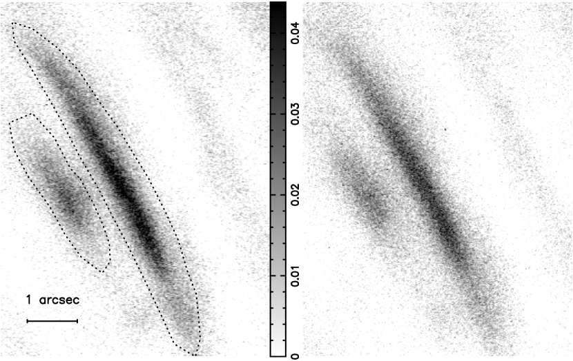
Figure 3: Enlarged $J$-band snapshots of the bright and faint wisps, taken on 2002 February 7, separated by $1.2\,{\rm ks}$. Orientation is as for Figure 1, with north up and east left. Each image has been background-subtracted and normalized to the flux of Star I. The gray scale is the same in both images and is indicated by the central bar. The units on the bar indicate the normalized flux (defined as in Figure 4) in a $1\arcsec\times 1\arcsec$ box. The apertures used to measure the total flux of the wisps, plotted in Figure 4, are drawn as dotted curves. The seeing and the guide star flux are the same in the two exposures to within $0.\arcsec 04$ and $4$ per cent respectively.

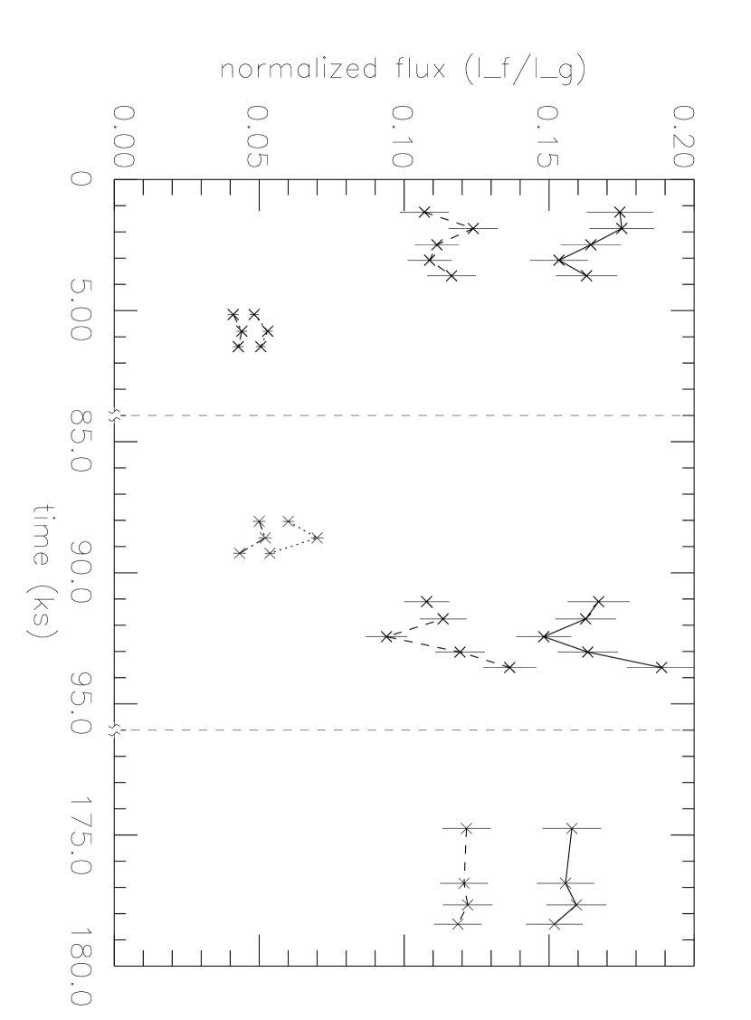
Figure 4: Light curves of the bright and faint wisps, after nebula subtraction and guide star normalization, as functions of time (in seconds) during the three nights of observations (demarcated by vertical lines). The four curves represent the bright wisp in $K^{\prime}$ (solid), faint wisp in $K^{\prime}$ (dashed), bright wisp in $J$ (dotted), and faint wisp in $J$ (dash-dotted).

Figure 3 shows two enlarged images of the bright and faint wisps in $J$ band, taken $1.2\,{\rm ks}$ apart on 2002 February 7, after nebula subtraction and normalization to the guide star ($I_{\rm f}/I_{\rm g}$; see §3.1). The frames should be identical if there is no change in the intrinsic brightness of the wisps, yet differences between them are readily apparent (although the features are not displaced). To quantify the changes, we use the polymark tool in IRAF to specify a polygonal aperture enclosing each wisp, as drawn in Figure 3. The fluxes enclosed by the apertures, after nebula subtraction and normalization, are plotted as functions of time in Figure 4. $J$- and $K^{\prime}$-band data are both displayed; uncertainties are calculated according to the recipe in §3.1. For the bright wisp, we find maximum flux changes (relative to the mean level) of $\pm 24\pm 4$ per cent in $J$ and $\pm 12\pm 7$ per cent in $K^{\prime}$, occurring in the space of $1.2\,{\rm ks}$ on 2002 February 7, and smaller fluctuations at other times. Moreover, the light curves of the bright and faint wisps appear correlated to some degree in both filters. The detection of variability is marginal in $K^{\prime}$ but more statistically significant in $J$, where the nebula background is less prominent. We find, by experimentation, that the results are essentially independent of the choice of aperture, while the time-dependent PSF has a minimal effect on the measured flux of the extended features (for the guide star, the effect is included in the measurement uncertainty; see §2). Nevertheless, new observations — preferably by an independent party using a different instrument — need to be made before variability of the wisps on such short time-scales can confidently be claimed.

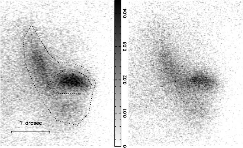
Figure 5: Enlarged $J$-band snapshots of the sprite (the fainter, larger feature on the left) and the rod (the brighter, smaller feature at center right), taken on 2002 February 7, separated by $1.2\,{\rm ks}$. Orientation is as for Figure 1, with north up and east left. Each image has been background-subtracted and normalized to the flux of Star I. The gray scale is the same in both images and is indicated by the central bar. The units on the bar indicate the normalized flux (defined as in Figure 4) in a $1\arcsec\times 1\arcsec$ box. The apertures used to measure the total fluxes of the sprite plus rod (plotted in Figure 6) and the rod alone (quoted in Table 1) are drawn as dotted polygons. The seeing and the guide star flux are the same in the two exposures to within $0.\arcsec 04$ and $4$ per cent respectively.

Figure 5 shows two enlarged images of the sprite in $J$ band, taken on 2002 February 6 and 8. It is interesting to note its doughnut-like structure, symmetric about the pulsar’s rotation axis, as well as the short, bent rod emerging from its center, seen clearly here for the first time and corroborating the observation by Hester et al. (2002) that the sprite is often center-filled (especially in X-rays). Knot-like features in another PWN, G320.4$-$1.2, numbered 2 and 3 by Gaensler et al. (2002), may be analogs of the sprite.

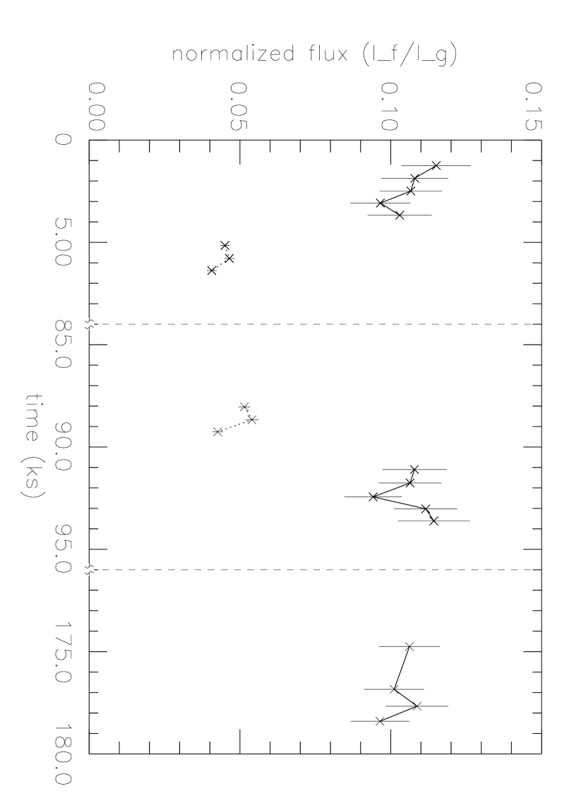
Figure 6: Light curve of the sprite, after nebula subtraction and guide star normalization, as a function of time (in seconds) during the three nights of observations (demarcated by vertical lines). The two curves represent $K^{\prime}$ (solid) and $J$ (dotted) data respectively.

In common with the wisps, there are visible differences in the brightness (but not the position) of the sprite in the two images, even after nebula subtraction and normalization — not just the absolute brightness, but also, more significantly, the brightness contrast between the rod and doughnut, which is less likely to be affected by PSF nonuniformity and imperfect sky/nebula subtraction. (The flux of the guide star is equal to within 4 per cent in the two snapshots.) To quantify the brightness changes, we define apertures enclosing the rod and the whole sprite, and plot the nebula-subtracted, normalized aperture flux $I_{\rm f}/I_{\rm g}$ versus time in Figure 6. We measure the following maximum flux changes (relative to the mean): $\pm 13\pm 4$ per cent (rod, $J$), $\pm 15\pm 7$ per cent (rod, $K^{\prime}$), $\pm 9\pm 4$ per cent (whole sprite, $J$), and $\pm 8\pm 7$ per cent (whole sprite, $K^{\prime}$). As for the wisps, the detection of variability is marginal in $K^{\prime}$ and somewhat more significant in $J$, especially for the rod, as seen in Figure 5.

3.3 Pulsar wind: inner knot

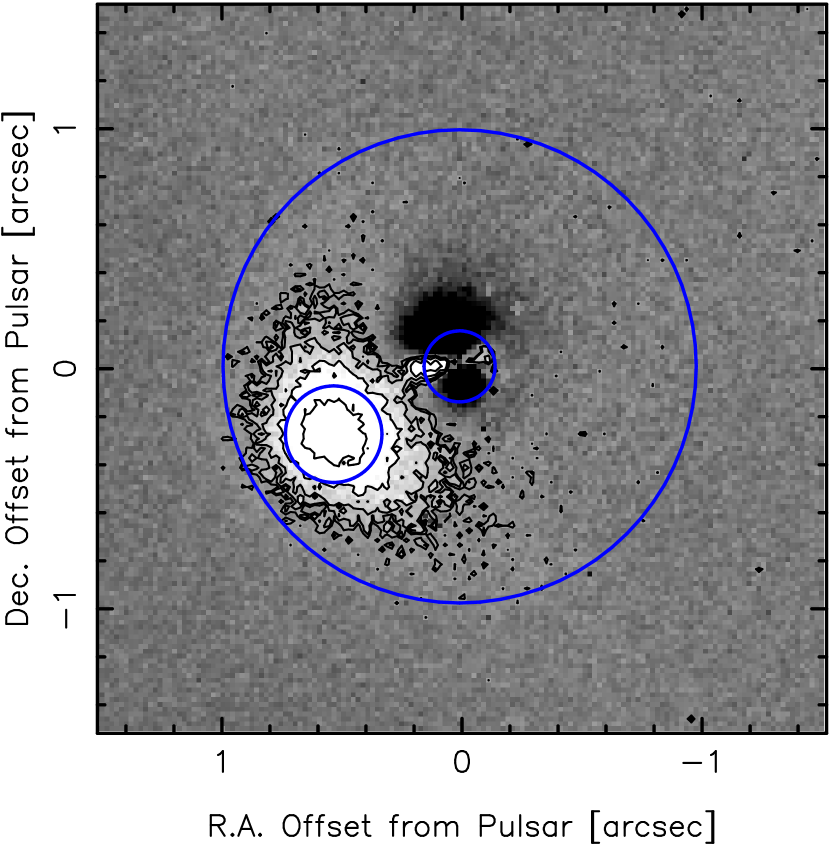
Figure 7: Enlarged $K^{\prime}$ image of the inner knot after subtraction of the pulsar PSF, plotted as a gray scale image with isophotes (solid contours) overlaid. The subtraction is imperfect because the PSF template is taken from the guide star, yet the PSF varies across the field of view (§2). Three apertures used in our photometry of the inner knot are also shown: two circles of radius $0.75$ ${\rm FWHM}$ and $5.0$ ${\rm FWHM}$, centered on the pulsar, and a circle of radius 10 pixels, centered on the brightness centroid of the inner knot. An annular region of inner radius $6.0$ ${\rm FWHM}$ and one pixel width, also centered on the inner knot and used to estimate the background (§3.3), lies outside the borders of the image.

The inner knot, discovered by Hester et al. (1995) in optical HST data, is displaced $0.\arcsec 65$ from the pulsar along the axis of symmetry of the PWN, and is resolved by HST to be $\approx 0.\arcsec 2$ thick (Hester et al., 1995). No counterpart has been detected unambiguously at X-ray wavelengths, although there is a hint of a southeasterly ‘bump’ protruding from the pulsar in CXO images, e.g. in Figure 5 of Hester et al. (2002). It is also possible that an analogous feature, named feature 1, has been discovered in CXO images of another PWN, G320.4$-$1.2 (Gaensler et al., 2002). In Figure 7, we present a brightness map of the inner knot, after subtraction of the PSF. It is clear, from the isophotes (solid contours) in particular, that the feature is flattened, not spherical, although it is hard to discern its shape exactly because it is barely resolved in our highest-resolution $K^{\prime}$ data and the PSF subtraction is imperfect.

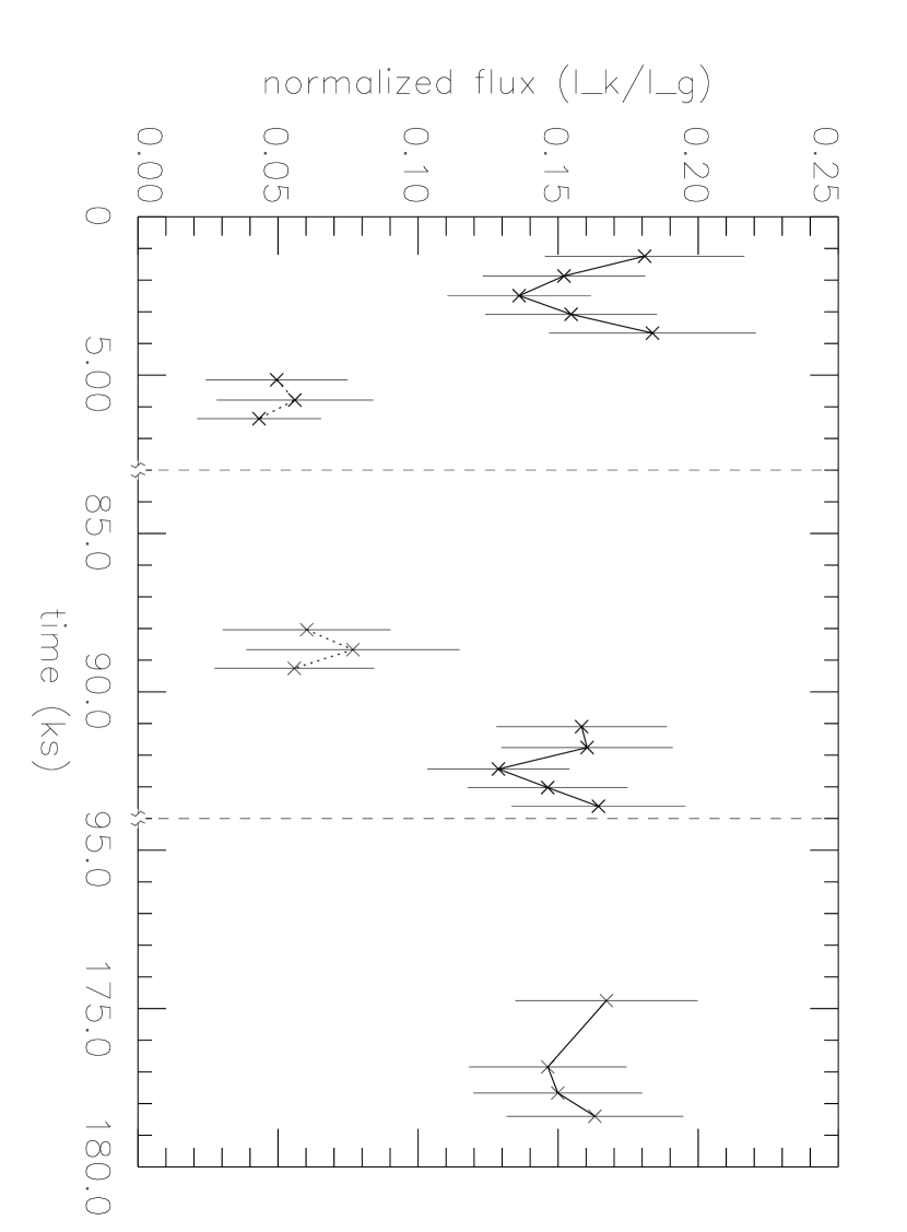
Figure 8: Light curve of the inner knot, plotted as the flux ratio difference $I_{\rm k}/I_{\rm g}=I_{\rm p}(r_{2})/I_{\rm g}(r_{2})-I_{\rm p}(r_{1})/I_{\rm g}(r_{1})$ for apertures with $r_{1}=0.75$ ${\rm FWHM}$ and $r_{2}=5.0$ ${\rm FWHM}$. The two curves represent $K^{\prime}$ (solid) and $J$ (dotted) data respectively.

Photometry of the inner knot is complicated by its proximity to the pulsar, whose flux contaminates the knot unpredictably from image to image as the seeing fluctuates. The standard approach, modeling and subtracting the pulsar PSF, is attempted in Figure 7, but the result is unreliable; see §2. Faced with these difficulties, we test for variability of the inner knot without measuring its brightness directly in two complementary ways. In the first test, we measure the fluxes $I_{\rm p}(r_{1})$ and $I_{\rm p}(r_{2})$ (after subtracting $\langle I_{\rm o}^{\prime}\rangle$) enclosed by two circular apertures centered on the pulsar, of radii $r_{1}=0.75$ ${\rm FWHM}$ (including as much PSF as possible but excluding most of the knot) and $r_{2}=5.0$ ${\rm FWHM}$ (including the PSF and knot). The apertures are drawn in Figure 7. The ratio of these fluxes, after nebula subtraction, would be the same as the ratio of the fluxes $I_{\rm g}(r_{1})$ and $I_{\rm g}(r_{2})$ enclosed by identical apertures around the guide star if there were no inner knot, because the cylindrically averaged PSF is uniform to within $\pm 6$ ($\pm 4$) per cent in $K^{\prime}$ ($J$) across the field of view (see §2). Therefore, the flux difference $I_{\rm k}/I_{\rm g}=I_{\rm p}(r_{2})/I_{\rm g}(r_{2})-I_{\rm p}(r_{1})/I_{\rm g}(r_{1})$ can be attributed to the presence of the inner knot, and any change in $I_{\rm k}/I_{\rm g}$ from image to image is evidence that the inner knot varies intrinsically. In Figure 8, we plot $I_{\rm k}/I_{\rm g}$ as a function of time for the full sequence of observations. The data are consistent with no variability, within the measurement uncertainties. For example, in the $K^{\prime}$ band, we find maximum peak-to-peak changes in $I_{\rm k}/I_{\rm g}$ of $0.045\pm 0.060$ over $1.2\,{\rm ks}$ and $0.054\pm 0.063$ over $48$ hours.

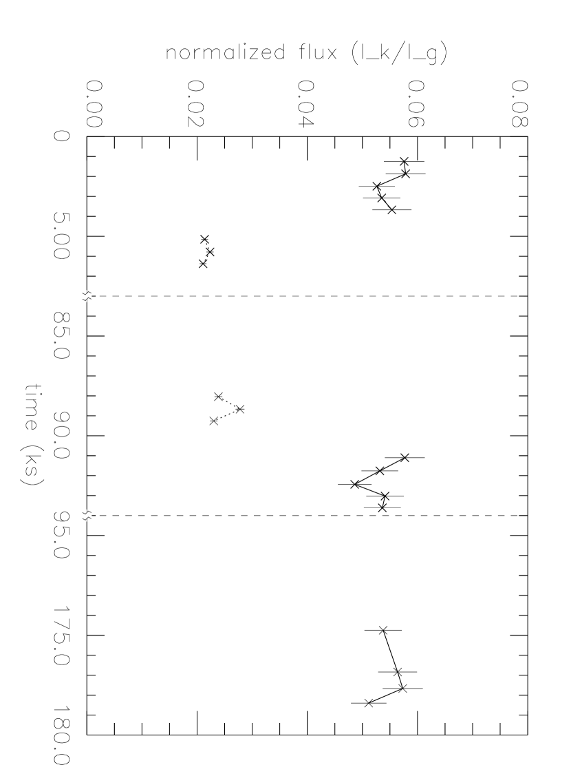
Figure 9: Light curve of the inner knot, plotted as the flux enclosed by a circular aperture of radius 10 pixels (after nebula subtraction and guide star normalization). This aperture includes some leakage from the pulsar PSF. The two curves represent $K^{\prime}$ (solid) and $J$ (dotted) data respectively.

A second test provides a consistency check: we measure directly the flux enclosed by a circular aperture of radius 10 pixels, centered on the knot. The flux thus measured includes leakage from the pulsar PSF, the amount of which varies from image to image along with the seeing, as noted above, but strong intrinsic variations in knot brightness could still overwhelm this effect. In Figure 9, we plot the flux in the 10-pixel aperture as a function of time, after nebula subtraction and guide star normalization. The result is consistent with Figure 8: there is no significant detection of variability within the measurement uncertainties, with a maximum peak-to-peak change of $0.011\pm 0.007$ over $1.2\,{\rm ks}$ on 2002 February 7.

On the strength of the data presented here, we are unable to say whether or not the inner knot is variable on time-scales of $0.6\,{\rm ks}$ to $48$ hours. New observations — preferably by an independent party using a different instrument — are required to settle the issue, and dedicated PSF calibration frames will be essential if adaptive optics are used.

4 Feature-specific color spectra

4.1 Near infrared: wisps, sprite, and inner knot

In this section, we measure the $J$-to-$K^{\prime}$ color spectra of the faint wisp, bright wisp, sprite, rod, and inner knot. As these features may vary on time-scales shorter than the minimum interval between exposures, we sum the 14 $K^{\prime}$ images and 6 $J$ images in our data set to obtain time-averaged spectra.

To the best of our knowledge, calibrated $J$-to-$K^{\prime}$ spectra of Stars I and II have not been published. Therefore, to calibrate the spectra of the various subarcsecond features in the PWN, we are forced to redo the photometry in §3 by normalizing nebula-subtracted fluxes with respect to the pulsar, whose phase-averaged, near-infrared, color spectrum was determined by Eikenberry et al. (1997) using the Solid State Photomultiplier on the Multiple Mirror Telescope. After dereddening, the pulsar’s spectrum is fairly flat in the near infrared ($F_{\nu}\propto\nu^{0.36}$); see the third row of Table 1. Note that the fluxes in Eikenberry et al. (1997) include the inner knot (unresolved from the ground). By comparing with the total flux of the pulsar plus knot in our images, we derive a zero magnitude reference for calibrated aperture photometry of the extended features (e.g. wisps, sprite, and rod).

To measure the flux of the knot, we remove the contribution from the pulsar by scaling it to the azimuthally averaged PSFs of Stars I and II, such that the normalization is the same at a radius of 10 pixels. The combined profile of the pulsar and knot is found to match the stellar PSFs up to a radius of $\approx 20$ pixels (to within $0.05\,{\rm mag}$ in $K^{\prime}$ and $0.03\,{\rm mag}$ in $J$) but deviates beyond due to the knot excess. We measure the flux difference between radii of 20 and 60 pixels (where the profile merges into the background) and adjust the results in Eikenberry et al. (1997) to give the calibrated knot flux. Note that the differential method of detecting the knot ($I_{\rm k}/I_{\rm g}$) employed in §3.3 does not yield a calibrated flux.

Time-averaged $J$- and $K^{\prime}$-band fluxes are presented in Table 1 for the point-like and extended subarcsecond features identified in Figure 1, together with the spectral index $\alpha$ of each feature assuming its flux density scales as $F_{\nu}\propto\nu^{\alpha}$ (as for synchrotron radiation, although not necessarily for all nonthermal processes, e.g. synchro-Compton radiation; see §5). The fluxes for the extended features are quoted per unit length, although it is possible that we are marginally resolving the wisps across their width. The field stars are included for reference, as their spectra have not been published previously. Three sources of uncertainty, summed in quadrature, contribute in Table 1. First, the central wavelength of the $K$ filter used by Eikenberry et al. (1997) is $0.08\,\mu{\rm m}$ greater than for the QUIRC $K^{\prime}$ filter. Second, there is scatter in the 20-pixel flux and 20-to-60-pixel offset. Third, the extinction corrections are uncertain ($0.63\pm 0.03\,{\rm mag}$ in $J$ and $0.81\pm 0.03\,{\rm mag}$ in $K^{\prime}$).

Several interesting conclusions emerge from these data. First, the inner knot is clearly the reddest feature in the region, with $\alpha\approx{-0.8}$. This is understandable if the inner knot is produced in the pulsar wind by a different radiation mechanism than other features. However, it is surprising if the inner knot is part of the same arch shock that produces the sprite. Second, the polar or mid-latitude sprite and rod have flatter spectra ($\alpha={-0.21\pm 0.13}$) than the equatorial wisps ($\alpha={-0.56\pm 0.12}$). Yet all these features are synchrotron emitting elements of the same termination shock, albeit at different latitudes. Third, there is no feature in the region whose spectrum matches smoothly from the near infrared to X-rays. The theoretical implications of these results are considered further in §5.

4.2 Ultraviolet: inner knot

We extend the spectrum of the inner knot in Table 1 with an independent measurement of the ultraviolet flux of this feature. Gull et al. (1998) observed the Crab pulsar with the HST Space Telescope Imaging Spectrograph (STIS) NUV-MAMA detector on 1997 August 7 through the low dispersion G230L grating. The observations were made using a $2\arcsec\times 2\arcsec$ aperture which included the inner knot, with part of the exposure ($2\times 2.4\,{\rm ks}$) in TIME-TAG mode. We acquired the archival data, barycentered the photons using standard STIS routines, and extracted a ‘slit’ image using photons from $0.25\,{\rm rad}$ of phase spanning the pulse minimum, thereby gating out the pulsar. Approximately two per cent of the unpulsed flux remained, but, after subtracting a scaled version of the on-pulse PSF, a clear excess was found at the projected position of the inner knot $\approx 0.3\pm 0.2\arcsec$ on one side of the pulsar. The intensity profile agrees with that expected from a one-dimensional collapse of direct HST images. Assuming a flat $\alpha\approx 0$ spectral index over the NUV band ($160$–$320\,{\rm nm}$), we find a summed inner knot flux $(3.3\pm 0.1)\times 10^{-2}$ times the unpulsed flux of the pulsar. De-reddening with the best fit value $E(B-V)=0.52$ (Sollerman et al., 2000) yields $F_{\nu}=0.12\pm 0.01\,{\rm mJy}$ for wavelengths in the range $0.16$–$0.32\,\mu{\rm m}$. Note that the ultraviolet flux is consistent with the near-infrared spectrum measured in §4.1, which extrapolates to give $F_{\nu}=0.11\,{\rm mJy}$ at $0.32\,\mu{\rm m}$ for $\alpha=-0.8$.

5 Discussion

In this paper, we report on the first near-infrared, adaptive-optics observations of the wisps and jet of the Crab PWN, comprising 20 $J$- and $K^{\prime}$-band snapshots taken at $0.\arcsec 19$–$0.\arcsec 37$ resolution with the Hokupa’a/QUIRC camera on the Gemini North Telescope. The data contain tantalizing — albeit inconclusive — evidence that subarcsecond features in the termination shock of the Crab PWN vary intrinsically in $J$-band brightness by $\pm 24\pm 4$ (wisps) and $\pm 14\pm 4$ (sprite) per cent on time-scales as short as $1.2\,{\rm ks}$. The principal sources of uncertainty are the nonuniform, unsteady nebula background and PSF. The data also suggest that the near-infrared spectra of polar features in the termination shock are flatter (e.g. sprite, $F_{\nu}\propto\nu^{-0.21\pm 0.13}$) than the spectra of the equatorial wisps ($F_{\nu}\propto\nu^{-0.56\pm 0.12}$), except for the steep-spectrum inner knot ($F_{\nu}\propto\nu^{-0.8}$), which may lie in the unshocked pulsar wind. This result is supported by an independent measurement of the ultraviolet flux of the inner knot, obtained by reanalyzing archival, time-tagged, HST STIS data.

5.1 Ion cyclotron and fire hose instabilities

Why, physically, might the nebula vary on time-scales as short as $1.2\,{\rm ks}$? According to one hypothesis, modeled numerically by Spitkovsky & Arons (2004), the wind contains ions which drive a relativistic cyclotron instability at the termination shock. The instability exhibits limit cycle dynamics: ion bunches and magnetic compressions are launched downstream periodically at roughly half the ion-cyclotron period, $\frac{1}{2}T_{\rm i}=\pi A_{\rm i}m_{\rm p}\gamma_{\rm i}/Z_{\rm i}eB$, where $A_{i}$ and $Z_{i}$ are the atomic number and charge, $\gamma_{i}$ is the preshock Lorentz factor, and $B$ is the postshock magnetic field. In order to fit the separation of the innermost wisps, one must take $T_{\rm i}\approx 3.2\times 10^{7}\,{\rm s}$, consistent with $\gamma_{\rm i}=7.8\times 10^{5}$ and $B=16\,\mu{\rm G}$ at a radial distance $r=0.1\,{\rm pc}$ from the pulsar (for $A_{\rm i}/Z_{\rm i}=1$) (Spitkovsky & Arons, 2004). Faster variability is expected nearer the pulsar, because the magnetic field in the wind scales as $B=16(r/0.1\,{\rm pc})^{-1}\,\mu{\rm G}$. However, we find $T_{\rm i}\approx 2\times 10^{7}\,{\rm s}$ and $T_{\rm i}\approx 2\times 10^{6}\,{\rm s}$ at the sprite ($r\approx 0.05\,{\rm pc}$) and inner knot ($r\approx 0.007\,{\rm pc}$) respectively, slower than the variability observed. Relativistic Doppler boosting does not improve the agreement; the time-scale $\propto\gamma_{\rm i}^{-2}$ is unchanged downstream ($\gamma_{\rm i}\sim 1$) and too short upstream ($\gamma_{\rm i}\sim 10^{6}$). The electron-cyclotron period, $T_{\rm e}=(m_{\rm e}Z_{\rm i}/m_{\rm p}A_{\rm i})T_{\rm i}$, does fall in the observed range, but it is hard to see how to maintain coherent limit-cycle dynamics in the electrons when they are randomized rapidly at the shock by ion-driven magnetosonic waves (Gallant & Arons, 1994; Spitkovsky & Arons, 2004). We are therefore inclined to rule out a cyclotron origin of the observed kilosecond variability in the near infrared.

The argument against a cyclotron origin of the kilosecond variability assumes that all the energy in the unstable (compressional) ion-cyclotron-magnetosonic waves resides in the fundamental. This need not be so. The frequency spectrum of the waves is quite flat in one-dimensional simulations (Hoshino et al., 1992); significant power is deposited at high harmonics (up to orders $\sim m_{\rm p}/m_{\rm e}$) provided that parametric three-wave decays do not destroy the coherence of the waves, a plausible concern in a realistic, three-dimensional plasma (J. Arons, private communication).

Another possible mechanism, applicable especially to the knots in the polar jet, is the relativistic fire hose instability, driven by anisotropy of the kinetic pressure parallel ($P_{\parallel}$) and perpendicular ($P_{\perp}$) to the magnetic field $B$. Noerdlinger & Yui (1969) showed that the growth time $T_{\rm fh}^{\prime}$ in the bulk frame of the jet (denoted by primes) is given by

$$\frac{1}{T_{\rm fh}^{\prime}}=\frac{eB^{\prime}}{m_{\rm e}\langle\gamma^{\prime}\rangle}\frac{1.3-B^{\prime 2}/[\mu_{0}(P^{\prime}_{\parallel}-P^{\prime}_{\perp})]}{(1+c^{2}/v_{\rm A}^{\prime 2})^{1/2}+8}~{},$$ (1)

where $\langle\gamma^{\prime}\rangle$ is the thermal Lorentz factor, $v_{\rm A}^{\prime 2}=B^{\prime 2}/\mu_{0}\rho^{\prime}$ is the Alfvén speed, and $\rho^{\prime}$ is the density of the cold ion background. As long as the condition $P_{\parallel}^{\prime}-P_{\perp}^{\prime}>0.77B^{\prime 2}/\mu_{0}$ is met, the minimum growth time is given by $T_{\rm fh,min}^{\prime}=0.14m_{\rm e}\langle\gamma^{\prime}\rangle/eB^{\prime}$ for $v_{\rm A}^{\prime}\gg c$. Upon Lorentz transforming to the observer’s frame, we obtain (i) $T_{\rm fh,min}=0.14m_{\rm e}\langle\gamma\rangle/eB$ if $B$ is radial in the jet, or (ii) $T_{\rm fh,min}=0.14\gamma_{\rm i}m_{\rm e}\langle\gamma\rangle/eB$ if $B$ is helical or toroidal in the jet, assuming $\langle\gamma\rangle\approx\gamma_{\rm i}\langle\gamma^{\prime}\rangle$. (The validity of the last assumption depends subtly on the exact form of the electron distribution.) Immediately upstream from the termination shock of the jet, we have $\langle\gamma\rangle=1$, $B=2.7\,\mu{\rm G}$, and $\gamma_{\rm i}=7.8\times 10^{5}$, implying $T_{\rm fh,min}=2.3\,{\rm ks}$ in scenario (ii). Immediately downstream from the termination shock, we have $\langle\gamma\rangle\approx 1\times 10^{6}$, $B=8\,\mu{\rm G}$, and $\gamma_{\rm i}=1.1$, implying $T_{\rm fh,min}\approx 1.1\,{\rm ks}$ in scenarios (i) and (ii) — intriguingly close to the observed time-scale. Note that the fire hose instability only occurs for $P_{\parallel}^{\prime}>P_{\perp}^{\prime}$; in the reverse situation, a mirror instability exists for $P_{\perp}^{\prime}-P_{\parallel}^{\prime}>8.9B^{\prime 2}/\mu_{0}$, with growth time $\sim T_{\rm fh}^{\prime}$. Gallant & Arons (1994) argued that $P_{\parallel}^{\prime}/P_{\perp}^{\prime}$ increases from zero to unity downstream from the shock — the adiabatic index $(3+P_{\parallel}^{\prime}/P_{\perp}^{\prime})/(2+P_{\parallel}^{\prime}/P_{\perp}^{\prime})$ decreases from 3/2 to 4/3 as pitch-angle scattering isotropizes the electrons — but $P_{\parallel}^{\prime}>P_{\perp}^{\prime}$ cannot be excluded.

Despite appearances, it is unlikely that the fire hose instability causes the unsteady, serpentine motions observed in the Vela X-ray jet on time-scales between one day and several weeks (Pavlov et al., 2003), because the growth time appears to be too short. We estimate $T_{\rm fh,min}=0.14\gamma_{\rm i}m_{\rm e}\langle\gamma\rangle/eB\approx 0.1(\sigma/10^{-3})^{1/2}\,{\rm ks}$, taking $\langle\gamma\rangle=7\times 10^{4}$ [pair multiplicity $\approx 10^{3}$; see Figure 17 of Hibschman & Arons (2001)] and $B=0.15\sigma^{1/2}\,{\rm mG}$ (radial or toroidal), where $\sigma$ is the ratio of Poynting to kinetic energy flux at the base of the jet. Pavlov et al. (2003) suggests an alternative scenario, in which the end of the jet is bent by an external wind while the knots in the body of the jet are produced by hydromagnetic (kink and sausage) instabilities on the local Alfvén time-scale.

Our time-lapse observations resolve the light-crossing time-scale of the smallest features in the field, e.g. $2.2$ days for $0.\arcsec 19$ at $2.0\,{\rm kpc}$. Therefore, if the kilosecond variability we observe is real, it must arise from (i) a pattern traveling at a superluminal phase speed, or (ii) relativistic Doppler boosting in the upstream collimated outflow ($\gamma_{\rm i}^{-2}$ times the light-crossing time-scale; cf. millisecond variability of unresolved gamma-ray bursters). Our results are consistent with previous observations that also detected significant variations on, or faster than, the light-crossing time-scale: Hester et al. (2002) observed the optical knots in the Crab PWN to vary over six days, and Pavlov et al. (2003) observed the X-ray jet in the Vela PWN to vary over just two days.

5.2 Radiation mechanisms

The near-infrared spectral indices displayed in Table 1 are curious in several respects. First, the inner knot has a steeper spectrum than every other feature in the region — not just in our data, where the $J$-band flux is uncertain to $\pm 50$ per cent, but also in data obtained with the Infrared Spectrometer And Array Camera on the VLT in $0.\arcsec 65$–$0.\arcsec 88$ natural seeing (Sollerman, 2003). One explanation is that the inner knot is physically different from the other features: the wisps and sprite are part of the termination shock and emit synchrotron radiation, e.g. from ion-cyclotron-heated electrons (Gallant & Arons, 1994), whereas the inner knot lies upstream in the unshocked pulsar wind and emits synchro-Compton radiation, e.g. from electrons heated by magnetic reconnection (Coroniti, 1990; Lyubarsky & Kirk, 2001) or parametric instabilities (Melatos & Melrose, 1996; Melatos, 1998, 2002) in a wave-like wind. This explanation conflicts with recent simulations which suggest that the inner knot is synchrotron emission from an arch shock between the polar outflow and equatorial backflow in the nebula (Komissarov & Lyubarsky, 2003). Unfortunately, we cannot discriminate between these two possibilities spectrally, because both synchrotron and synchro-Compton radiation yield $\alpha=(1-p)/2$ given a power-law electron distribution $N(\gamma)\propto\gamma^{-p}$ (Blandford, 1972; Leubner, 1982). [Monoenergetic electrons in a large-amplitude wave emit an inverse Compton spectrum $F_{\nu}\propto\nu$ at frequencies below $0.1\gamma^{2}a^{3}\Omega\sim 10^{16}\,{\rm Hz}$, where $a=1$–10 is the wave nonlinearity parameter (Melatos & Melrose, 1996; Melatos, 1998) and $\Omega$ is the pulsar spin frequency, but this low-frequency tail is modified to $F_{\nu}\propto\nu^{(1-p)/2}$ for power-law electrons.] Instead, we propose that the near-infrared polarizations of the inner knot and the sprite be measured. Theory predicts that synchrotron and synchro-Compton radiation are polarized perpendicular and parallel to the magnetic field respectively; one expects 50–80 per cent linear polarization from a linearly polarized large-amplitude wave if $0.5\leq p\leq 5$ (Blandford, 1972). Therefore, assuming that the magnetic geometry of the wave-like wind is similar at the inner knot and sprite (e.g. helical at high latitude), the polarization vectors of the two features are expected to be perpendicular if the inner knot originates from the unshocked pulsar wind and parallel if it is an arch shock. Moreover, if the inner knot originates from the unshocked wind, it should also be circularly polarized (degree $\sim a^{-1}$, independent of $\nu$).

A second curious property of the spectra in Table 1 is that the bright and faint wisps are steeper than the sprite and rod. In this case, there is no doubt that both sets of features are shock-related synchrotron emission at equatorial and polar latitudes respectively, whether the sprite is located at the working surface of the polar jet (Hester et al., 2002) or along the arch shock (Komissarov & Lyubarsky, 2003; Del Zanna et al., 2004). So why do the spectra differ? One possibility is that the polarization of the large-amplitude wave in the wind zone, which is linear at the equator and circular at the pole, affects the acceleration physics in the shock ponderomotively; tentative indications to this end are emerging from recent particle-in-cell simulations (O. Skjaeraasen, private communication).

Table 1 raises a third puzzle: the near-infrared spectra of some features do not extrapolate smoothly to optical and X-ray wavelengths, while others do. For example, the HST $V$-band surface brightness of the bright wisp and the $V$-band flux of the sprite are measured to be $49\,\mu{\rm Jy\,arcsec^{-1}}$ and $4.1\,\mu{\rm Jy}$ respectively (Hester et al., 1995); the same quantities, extrapolated from Table 1, are predicted to be $\approx 42\,\mu{\rm Jy\,arcsec^{-1}}$ and $\approx 15\,\mu{\rm Jy}$ respectively. VLT and HST observations show that the spectrum of the inner knot extends smoothly from near-infrared to optical wavelengths, with $\alpha=-0.75\pm 0.15$ (Sollerman, 2003), and this is corroborated (within larger uncertainties) by our data. On the other hand, extrapolation of the VLT spectrum of the inner knot to $0.16$–$0.32\,\mu{\rm m}$ yields $F_{\nu}=0.35\pm 0.05\,{\rm mJy}$, significantly greater than the ultraviolet flux measured in §4.2.

The spectrum of the bright and faint wisps is significantly steeper in X-rays than in the near infrared, with $\alpha_{\rm X}\approx-1.3$ (Weisskopf et al., 2000) and $\alpha_{\rm NIR}-\alpha_{\rm X}\approx 0.7$, comparable to the steepening expected from synchrotron cooling (Y. Lyubarsky, private communication). The synchrotron cooling time for near-infrared-emitting electrons, $t_{\rm cool}=2.8\times 10^{4}(B/16\,\mu{\rm G})^{-3/2}(\nu/2.4\times 10^{14}\,{\rm Hz})^{-1/2}\,{\rm yr}$, is much longer than the flow time $t_{\rm flow}$ across the wisps. On the other hand, the near-infrared spectral index of the sprite and rod ($\alpha=-0.21\pm 0.13$) is significantly shallower than the wisps and similar to the average radio spectral index of the nebula (Y. Lyubarsky, private communication). This is either coincidental or highly surprising. The sprite and rod are shock features in which one has $t_{\rm flow}\ll t_{\rm cool}$ for near-infrared-emitting electrons and kilosecond variability is observed; they reflect electron acceleration at the present time. The radio electrons reflect the history of electron acceleration over the lifetime of the nebula and should be unaffected by the present dynamics of the sprite. This paradox is encountered in a related context: Bietenholz et al. (2001) observed that the radio and optical wisps travel radially in concert and display coordinated spectral index variations.

We conclude by reiterating that the measurement uncertainties in our observations are substantial, due to the nonuniformity of the nebula and PSF. Consequently, the evidence for kilosecond variability and spectral differences, while tantalizing, is inconclusive. Improved observations — preferably by an independent party using a different instrument — are essential to clarify the situation.

Figure 1: Near-infrared image of the central $20\arcsec\times 20\arcsec$ region of the Crab PWN, constructed from four dithered, $0.12\,{\rm ks}$ exposures in the $K^{\prime}$ filter, taken on 2002 February 6 with a resolution of ${\rm FWHM}=0.\arcsec 19$. The principal features of the pulsar wind termination shock and its environment are labeled, revealing the ‘crossbow’ morphology characteristic of many PWN: arc-like, equatorial wisps and jet-like, polar knots symmetric about the projected rotation axis of the pulsar. Star I is the Hokupa’a guide star. Star II is another field star.

Figure 2: Statistics of the nebula background. $a$. Left. Frequency histogram of pixel counts in a typical $K^{\prime}$ image constructed from $4\times 0.12{\rm ks}$ dithered exposures on 2002 February 6, excluding point sources and extended features. Raw counts (solid curve) and counts averaged over $50\times 50$ pixel blocks (dashed curve) are shown; the curves overlap and are indistinguishable to the eye. $b$. Right. Frequency histogram of pixel counts in an annulus, radius $6.0{\rm FWHM}$ and one pixel thick, centered on the guide star (Star I).

Point source	$J$ flux	$K^{\prime}$ flux	$\alpha$	length
	[mJy]	[mJy]		[arcsec]
Star I	6.25 (0.12)	3.09 (0.07)	$1.24$	—
Star II	1.01 (0.02)	0.76 (0.02)	$0.50$	—
Pulsar	3.21 (0.15)	2.62 (0.17)	$0.36$	—
Knot	0.32 (0.16)	0.49 (0.17)	$-0.78$	—
Extended feature	$J$ flux	$K^{\prime}$ flux	$\alpha$	length
	[$\mu$Jy arcsec-1]	[$\mu$Jy arcsec-1]		[arcsec]
Bright wisp	69.4 (1.4)	97.7 (2.2)	$-0.60$	7.3
Faint wisp	59.8 (1.3)	80.3 (1.8)	$-0.52$	3.3
Rod	62.8 (1.3)	68.7 (1.6)	$-0.16$	1.2
Sprite	46.2 (1.0)	53.5 (1.2)	$-0.26$	2.5

Table 1: De-reddened fluxes and power-law spectral indices ($F_{\nu}\propto\nu^{\alpha}$) for features present in the images, collected into point sources (including the inner knot; top) and extended features (bottom). Fluxes for the extended features are quoted per arcsecond of length; the lengths are shown in the right-hand column. Errors ($1\sigma$) are quoted in parentheses after the fluxes. A correction has been made for interstellar extinction (Eikenberry et al. 1997).

References

- Begelman (1998) Begelman, M. C. 1998, ApJ, 493, 291
- Begelman (1999) —. 1999, ApJ, 512, 755
- Begelman & Li (1992) Begelman, M. C., & Li, Z. 1992, ApJ, 397, 187
- Begelman & Li (1994) —. 1994, ApJ, 426, 269
- Bietenholz et al. (2001) Bietenholz, M. F., Frail, D. A., & Hester, J. J. 2001, ApJ, 560, 254
- Blandford (1972) Blandford, R. D. 1972, A&A, 20, 135
- Bogovalov (2001) Bogovalov, S. V. 2001, A&A, 371, 1155
- Caraveo & Mignani (1999) Caraveo, P. A., & Mignani, R. P. 1999, A&A, 344, 367
- Coroniti (1990) Coroniti, F. V. 1990, ApJ, 349, 538
- Del Zanna et al. (2004) Del Zanna, L., Amato, E., & Bucciantini, N. 2004, A&A, 421, 1063
- Eikenberry et al. (1997) Eikenberry, S. S., Fazio, G. G., Ransom, S. M., Middleditch, J., Kristian, J., & Pennypacker, C. R. 1997, ApJ, 477, 465
- Gaensler et al. (2002) Gaensler, B. M., Arons, J., Kaspi, V. M., Pivovaroff, M. J., Kawai, N., & Tamura, K. 2002, ApJ, 569, 878
- Gaensler et al. (2001) Gaensler, B. M., Pivovaroff, M. J., & Garmire, G. P. 2001, ApJ, 556, L107
- Gallant & Arons (1994) Gallant, Y. A., & Arons, J. 1994, ApJ, 435, 230
- Gotthelf & Wang (2000) Gotthelf, E. V., & Wang, Q. D. 2000, ApJ, 532, L117
- Graves et al. (1998) Graves, J. E., Northcott, M. J., Roddier, F. J., Roddier, C. A., & Close, L. M. 1998, in Proc. SPIE Vol. 3353, p. 34-43, Adaptive Optical System Technologies, Domenico Bonaccini; Robert K. Tyson; Eds., Vol. 3353, 34–43
- Gull et al. (1998) Gull, T. R., Lindler, D. J., Crenshaw, D. M., Dolan, J. F., Hulbert, S. J., Kraemer, S. B., Lundqvist, P., Sahu, K. C., Sollerman, J., Sonneborn, G., & Woodgate, B. E. 1998, ApJ, 495, L51+
- Hester et al. (2002) Hester, J. J., Mori, K., Burrows, D., Gallagher, J. S., Graham, J. R., Halverson, M., Kader, A., Michel, F. C., & Scowen, P. 2002, ApJ, 577, L49
- Hester et al. (1995) Hester, J. J., Scowen, P. A., Sankrit, R., Burrows, C. J., Gallagher, J. S., Holtzman, J. A., Watson, A., Trauger, J. T., Ballester, G. E., Casertano, S., Clarke, J. T., Crisp, D., Evans, R. W., Griffiths, R. E., Hoessel, J. G., Krist, J., Lynds, R., Mould, J. R., O’Neil, E. J., Stapelfeldt, K. R., & Westphal, J. A. 1995, ApJ, 448, 240
- Hibschman & Arons (2001) Hibschman, J. A., & Arons, J. 2001, ApJ, 560, 871
- Hoshino et al. (1992) Hoshino, M., Arons, J., Gallant, Y. A., & Langdon, A. B. 1992, ApJ, 390, 454
- Kaspi et al. (2001) Kaspi, V. M., Roberts, M. E., Vasisht, G., Gotthelf, E. V., Pivovaroff, M., & Kawai, N. 2001, ApJ, 560, 371
- Komissarov & Lyubarsky (2003) Komissarov, S. S., & Lyubarsky, Y. E. 2003, MNRAS, 344, L93
- Leubner (1982) Leubner, C. 1982, ApJ, 253, 859
- Lu et al. (2002) Lu, F. J., Wang, Q. D., Aschenbach, B., Durouchoux, P., & Song, L. M. 2002, ApJ, 568, L49
- Lyubarsky & Eichler (2001) Lyubarsky, Y., & Eichler, D. 2001, ApJ, 562, 494
- Lyubarsky & Kirk (2001) Lyubarsky, Y., & Kirk, J. G. 2001, ApJ, 547, 437
- Lyubarsky (2002) Lyubarsky, Y. E. 2002, MNRAS, 329, L34
- Melatos (1998) Melatos, A. 1998, Memorie della Societa Astronomica Italiana, 69, 1009
- Melatos (2002) Melatos, A. 2002, in ASP Conf. Ser. 271: Neutron Stars in Supernova Remnants, 115–+
- Melatos (2004) Melatos, A. 2004, in IAU Symposium 218: Young Neutron Stars and their Environments, 143–+
- Melatos & Melrose (1996) Melatos, A., & Melrose, D. B. 1996, MNRAS, 279, 1168
- Mori et al. (2002) Mori, K., Hester, J. J., Burrows, D. N., Pavlov, G. G., & Tsunemi, H. 2002, in ASP Conf. Ser. 271: Neutron Stars in Supernova Remnants, 157–+
- Noerdlinger & Yui (1969) Noerdlinger, P. D., & Yui, A. K. 1969, ApJ, 157, 1147
- Pavlov et al. (2001) Pavlov, G. G., Kargaltsev, O. Y., Sanwal, D., & Garmire, G. P. 2001, ApJ, 554, L189
- Pavlov et al. (2003) Pavlov, G. G., Teter, M. A., Kargaltsev, O., & Sanwal, D. 2003, ApJ, 591, 1157
- Slane et al. (2002) Slane, P. O., Helfand, D. J., Murray, S. S., & Gotthelf, E. V. 2002, in American Astronomical Society Meeting 201, #139.04, Vol. 201, 0–+
- Sollerman (2003) Sollerman, J. 2003, A&A, 406, 639
- Sollerman et al. (2000) Sollerman, J., Lundqvist, P., Lindler, D., Chevalier, R. A., Fransson, C., Gull, T. R., Pun, C. S. J., & Sonneborn, G. 2000, ApJ, 537, 861
- Spitkovsky & Arons (2004) Spitkovsky, A., & Arons, J. 2004, ApJ, 603, 669
- Usov (1994) Usov, V. V. 1994, MNRAS, 267, 1035
- Weisskopf et al. (2000) Weisskopf, M. C., Hester, J. J., Tennant, A. F., Elsner, R. F., Schulz, N. S., Marshall, H. L., Karovska, M., Nichols, J. S., Swartz, D. A., Kolodziejczak, J. J., & O’Dell, S. L. 2000, ApJ, 536, L81