HST STIS Spectroscopy of the Triple Nucleus of M 31:
Two Nested Disks in Keplerian Rotation around a Supermassive Black Hole

Abstract

We present Hubble Space Telescope (HST) spectroscopy of the nucleus of M 31 obtained with the Space Telescope Imaging Spectrograph (STIS). Spectra that include the Ca II infrared triplet ($\lambda\simeq 8500$ Å) see only the red giant stars in the double brightness peaks P1 and P2. In contrast, spectra taken at $\lambda\lambda\simeq$ 3600 – 5100 Å are sensitive to the tiny blue nucleus embedded in P2, the lower-surface-brightness nucleus of the galaxy. P2 has a K-type spectrum, but we find that the blue nucleus has an A-type spectrum – it shows strong Balmer absorption lines. Hence, the blue nucleus is not blue because of AGN light but rather because it is dominated by hot stars. We show that the spectrum is well described by A0 giant stars, A0 dwarf stars, or a 200-Myr-old, single-burst stellar population. White dwarfs, in contrast, cannot fit the blue nucleus spectrum. Given the small likelihood for stellar collisions, recent star formation appears to be the most plausible origin of the blue nucleus. In stellar population, size, and velocity dispersion, the blue nucleus is so different from P1 and P2 that we call it P3 and refer to the nucleus of M 31 as triple.

Because P2 and P3 have very different spectra, we can make a clean decomposition of the red and blue stars and hence measure the light distribution and kinematics of each uncontaminated by the other. The line-of-sight velocity distributions of the red stars near P2 strengthen the support for Tremaine’s (1995) eccentric disk model. Their wings indicate the presence of stars with velocities of up to $~{}1000$ km s^-1 on the anti-P1 side of P2.

The kinematic properties of P3 are consistent with a circular stellar disk in Keplerian rotation around a supermassive black hole. If the P3 disk is perfectly thin, then the inclination angle $i\simeq 55^{\circ}$ is identical within the errors to the inclination of the eccentric disk models for P1 $+$ P2 by Peiris & Tremaine (2003) and by Salow & Statler (2004). Both disks rotate in the same sense and are almost coplanar. The observed velocity dispersion of P3 is largely caused by blurred rotation and has a maximum value of $\sigma=1183\pm 201$ km s^-1. This is much larger than the dispersion $\sigma\simeq 250$ km s^-1 of the red stars along the same line of sight and is the largest integrated velocity dispersion observed in any galaxy. The rotation curve of P3 is symmetric around its center. It reaches an observed velocity of $V=618\pm 81$ km s^-1 at radius 0$\farcs$05 = 0.19 pc, where the observed velocity dispersion is $\sigma=674\pm 95$ km s^-1. The corresponding circular rotation velocity at this radius is $\sim$ 1700 km s^-1. We therefore confirm earlier suggestions that the central dark object interpreted as a supermassive black hole is located in P3.

Thin disk and Schwarzschild models with intrinsic axial ratios $b/a$ ${}_{<}\atop{{}^{\sim}}$ 0.26 corresponding to inclinations between $55^{\circ}$ and $58^{\circ}$ match the P3 observations very well. Among these models, the best fit and the lowest black hole mass are obtained for a thin disk model with $M_{\bullet}=1.4\times 10^{8}\,M_{\odot}$. Allowing P3 to have some intrinsic thickness and considering possible systematic errors, the 1-$\sigma$ confidence range becomes (1.1 to 2.3) $\times 10^{8}\,M_{\odot}$. The black hole mass determined from P3 is independent of but consistent with Peiris & Tremaine’s mass estimate based on the eccentric disk model for P1 $+$ P2. It is $\sim$ 2 times larger than the prediction by the correlation between $M_{\bullet}$ and bulge velocity dispersion $\sigma_{\rm bulge}$. Taken together with other reliable black hole mass determinations in nearby galaxies, notably the Milky Way and M 32, this strengthens the evidence that the $M_{\bullet}$ – $\sigma_{\rm bulge}$ relation has significant intrinsic scatter, at least at low black hole masses.

We show that any dark star cluster alternative to a black hole must have a half-mass radius ${}_{<}\atop{{}^{\sim}}$ $0\farcs 03=0.11$ pc in order to match the observations. Based on this, M 31 becomes the third galaxy (after NGC 4258 and our Galaxy) in which clusters of brown dwarf stars or dead stars can be excluded on astrophysical grounds.

1. Introduction

M 31 was the second galaxy in which stellar dynamics revealed the presence of a supermassive black hole (BH) (Kormendy 1987, 1988; Dressler & Richstone 1988). The spatial resolution of the discovery spectra was FWHM $\sim$ 1″. Axisymmetric dynamical models implied BH masses of $M_{\bullet}=(1~{}\rm to~{}10)\times 10^{7}$ $M_{\odot}$. The smallest masses were given by disk models and the largest were given by spherical models.

In 1988, it was already known that axisymmetry is only an approximation to a more complicated structure. With Stratoscope II, Light et al. (1974) had observed that the nucleus is asymmetric. The brightest point is offset both from the center of the bulge (Nieto et al. 1986) and from the velocity dispersion peak (Dressler 1984; Dressler & Richstone 1988; Kormendy (1988). Then, using HST, Lauer et al. (1993) discovered that the nucleus is double. The brighter nucleus, P1, is offset from the bulge center by $\sim 0\farcs 5$. The fainter nucleus, P2, is approximately at the bulge center. Early concerns that an apparently double structure might only be due to dust were laid to rest when infrared images proved consistent with optical and ultraviolet images (Mould et al. 1989; Rich et al. 1996; Davidge et al. 1997; Corbin, O’Neil, & Rieke 2001). These results were confirmed at higher resolution and signal-to-noise using WFPC2 (Lauer et al. 1998). With the discovery of the double nucleus, work on the central parts of M 31 went into high gear.

Bacon et al. (1994, 2001) used integral-field spectroscopy to map the two-dimensional velocity field near the center of M 31. They found that the kinematical major axis of the nucleus is not the same as the line that joins P1 and P2. The rotation curve is approximately symmetric about P2, i. e., about the center of the bulge. However, this is not the point of maximum dispersion. Instead, the brightest and hottest points are displaced from the rotation center by similar amounts in opposite directions.

The above results created two acute needs. First, the rich phenomenology of the double nucleus cried out for explanation. Second, the P1 – P2 asymmetry raised doubts about BH mass measurements. This paper is mainly about the BH. HST allows us to take an important step inward by studying a blue cluster of stars embedded in P2. We introduce this cluster in § 1.1. Second, our spectroscopy of P1 $+$ P2 (§§ 2 and 3) provides further support for the preferred model of the double nucleus (Appendix). Since that model affects much of our discussion, we summarize it in § 1.2. For comprehensive reviews, see Peiris & Tremaine (2003) and Salow & Statler (2004).

1.1. P3: The Blue Star Cluster Embedded in P2

Nieto et al. (1986), using a photon-counting detector on the Canada-France-Hawaii Telescope (CFHT), were the first to illustrate that P2 is brighter than P1 at 3750 Å (contrast their Figure 3 with Figure 4 in Light et al. 1974; cf. Figure 3 here). However, they did not realize this. Instead, they focused on the strong color gradient – bluer inward – and worried because this was inconsistent with published data. But these data were taken in the red or else had poor spatial resolution; they could not have seen the ultraviolet center. Nieto and collaborators found no problem with their data but concluded that “Further observations are required to settle this question.”

King et al. (1992) confirmed the ultraviolet excess in the nucleus using the HST Faint Object Camera (FOC) at 1750 Å. Using the same image, Crane et al. (1993b) illustrated that P2 is brighter than P1 but did not comment on this. Bertola et al. (1995) illustrated the same effect using FOC $+$ F150W $+$ F130LP images but again did not comment that it is P2, not P1, that is brighter in the ultraviolet.

Therefore, it was King, Stanford & Crane (1995) who discovered that P2 is much brighter than P1 in the ultraviolet. This result was again based on the 1750 Å FOC images. The blue light comes from a compact source that is embedded in P2 and that is similar in color and brightness to post-asymptotic-giant-branch (PAGB) stars seen elsewhere in the bulge (King et al. 1992; Bertola et al. 1995). King et al. (1995) proposed that the source might be nonthermal light from the weak AGN that is detected in the radio (Crane et al. 1992, 1993a), although they recognized that it could be a single PAGB star. Subsequently, Lauer et al. (1998) and Brown et al. (1998) resolved the source; its half-power radius is $\simeq$ 0$\farcs$06 = 0.2 pc. Both papers argued that it is a cluster of stars. Lauer et al. (1998) combined the King et al. (1995) UV fluxes with optical fluxes to conclude that the source is consistent with an A-star spectrum.

In this paper we present STIS spectra and show directly that the source is composed of A stars (§ 4). We also demonstrate that it is most consistent with a disk structure rather than with a dynamically hot cluster (§§ 5, 6). Because the blue cluster is so distinct from P1 $+$ P2 in terms of stellar content and kinematics, we call it P3 and refer to the nucleus of M 31 as triple.

The disk structure of P3 allows us to make a new and more reliable measurement of the central dark mass (§ 7). From the kinematics of P3 we also show that the dark object must be confined inside a radius $r$ ${}_{<}\atop{{}^{\sim}}$ 0$\farcs$03 = 0.11 pc. This implies that alternatives to a BH, such as a cluster of brown dwarf stars or stellar remnants, are inconsistent with the observations (§ 8).

1.2. The Eccentric Disk Model of P1 $+$ P2

Tremaine (1995) proposed what is now the standard model of P1 and P2. His motivation was the realization (see also Emsellem & Combes 1997) that the simplest alternative – an almost-completed merger – is implausible. Two clusters in orbit around each other at a projected separation of $0\farcs 49=1.8$ pc would merge in ${}_{<}\atop{{}^{\sim}}$$10^{8}$ yr by dynamical friction. Instead, Tremaine proposed that both nuclei are parts of the same eccentric disk of stars. The brighter nucleus, P1, is farther from the BH and results from the lingering of stars near apocenter. The fainter nucleus, P2, is explained by increasing the disk density toward the center. A BH is required in P2 to make the potential almost Keplerian; only then might the alignment of orbits be maintained by the modest self-gravity of the disk.

Statler et al. (1999), Kormendy & Bender (1999, hereafter KB), and Bacon et al. (2001) showed that the nucleus has the signature of the eccentric disk model. The most direct evidence is the asymmetry in $V(r)$ and $\sigma(r)$. Eccentric disk stars should linger at apocenter in P1; $V$ and $\sigma$ are observed to be relatively small there. The same stars should pass pericenter in P2, slightly on the anti-P1 side of the BH; the velocity amplitude is observed to be high on the anti-P1 side of the blue cluster. Because the PSF and the slit blur light from stars seen at different radii and viewing geometries, the apparent velocity dispersion should also have a sharp peak slightly on the anti-P1 side of the BH. All of the above papers demonstrated that the dispersion has a sharp peak in P2. KB showed further that the $\sigma$ peak is slightly on the anti-P1 side of the blue cluster. Therefore, they suggested that the BH is in the blue cluster. Finally, KB demonstrated that the spectra and metal line strengths of P1 and P2 are similar to each other but different from those of the bulge. Therefore P1 cannot be an accreted globular cluster or dwarf galaxy.

Peiris & Tremaine (2003) refined the eccentric disk model to optimize the fit to the higher-resolution and more detailed ground-based spectroscopy now available. Even the Gauss-Hermite coefficients $h_{3}$ and $h_{4}$ – which were not used in constructing the model – were adequately well fitted. These models were then used to predict the kinematics that should be observed in our Ca triplet HST spectra of the red stars. This is a stringent test because the new models were used to predict observations taken at much higher resolution than those used to construct the models. Excellent fits were obtained. This is a resounding success of the eccentric disk model. The structural and velocity asymmetries of the nucleus can be explained almost perfectly if the eccentric disk is inclined with respect to the plane of the outer disk of M 31. Here, we publish the kinematic data used by Peiris & Tremaine (2003) in the above comparison (§ 3), and we revisit particularly interesting features of the STIS kinematics of P1 $+$ P2 in the Appendix.

The main shortcoming of the Peiris & Tremaine models is that they do not include the self-gravity of the stars in the eccentric disk. If the disk has a mass of 10 % of the BH, then self-gravity is needed to keep the model aligned (Statler 1999). The most detailed such models are by Salow & Statler (2001, 2004). They model all available observations but do not fit the data as well as the models by Peiris & Tremaine (2003). Other self-consistent models are based on $N$-body simulations (Bacon et al. 2001, Jacobs & Sellwood 2001); again, they reproduce only some of the observations. Sambhus & Sridhar (2002) use the Schwarzschild (1979) method to model the double nucleus. The above models differ in many details. For example, the Salow and Statler models precess rapidly, with pattern speeds of $36\pm 4$ km s^-1 pc^-1; the models of Sambhus & Sridhar precess at 16 km s^-1 pc^-1, and the simulations of Bacon et al. (2001) precess at only 3 km s^-1 pc^-1. Not surprisingly, the construction of dynamical models that include self-gravity is a challenge. The conclusion that such models are long-lived is less secure than the result that they can instantaneously fit the photometry and kinematics of P1 $+$ P2. Tremaine (2001) gives a general discussion of slowly precessing eccentric disks.

Because of these complications, the BH mass in M 31 has remained uncertain. Estimates of $M_{\bullet}$ by Dressler et al. (1988), Kormendy (1988), Richstone et al. (1990), Bacon et al. (1994), Magorrian et al. (1998), KB, Bacon et al. (2001), Peiris & Tremaine (2003), and Salow & Statler (2004) have ranged over a factor of about 3, $M_{\bullet}\simeq(3~{}\rm to~{}10)\times 10^{7}$ $M_{\odot}$. These results are reviewed and error bars are tabulated on a uniform distance scale ($D=0.76$ Mpc) in Kormendy (2004). In this paper we show that an analysis of the UV-bright nucleus P3 allows us to estimate the black hole mass independent of P1 $+$ P2.

2. STIS Spectroscopy

The STIS CCD observations of M 31 were obtained on 1999 July 23 – 24. The slit was aligned at P.A. = $39\arcdeg$. Other details of the STIS configuration are given in Table 1. We obtained a spectrum that includes the calcium triplet, $\lambda\lambda$ 8498, 8542, and 8662 Å, and one at $\lambda\lambda$ 2700 – 5200 Å that includes several Balmer lines and Ca II H and K ($\lambda\lambda$ 3933 and 3968 Å). Both wavelength regions were observed because we wanted separately to analyze the double nucleus P1 $+$ P2 and the central blue cluster P3. Figure 1 shows that the double nucleus P1 $+$ P2 contributes almost all of the light at red wavelengths, while P3 dominates at 3000 Å. The color difference between P1 $+$ P2 and P3 is illustrated further in the brightness cuts in Figure 3. The red spectrum was obtained using the $52\times 0\farcs 1$ slit, while the blue spectrum was taken with the $52\times 0\farcs 2$ slit. A wider slit was chosen for the blue spectrum to ensure that P3 would fall inside the slit. Figure 1 shows the placement of the slit relative to the WFPC2 F555W and F300W images from Lauer et al. (1998). These slit positions were determined by comparing the light profiles along the slit in our STIS spectra with brightness cuts through the WFPC2 images. We measured the slit positions to an accuracy of $0\farcs 005$ for the red spectrum and $0\farcs 01$ for the blue spectrum. The total integration time for the red spectrum was split into two exposures of approximately 1200 s each per HST orbit. M 31’s nucleus was shifted by 4.1 pixels along the slit between orbits.

The total integration time for the blue spectrum was split into three equal exposures within one HST orbit. The nucleus was shifted by 4.3 pixels between successive exposures. Wavecals were interspersed among the galaxy exposures to allow wavelength calibration, including correction for thermal drifts. For the red spectrum, we obtained contemporaneous flat-field exposures through the same slit while M 31 was occulted by the Earth. These provide proper calibration of internal fringing, which is significant at $\lambda\geq 7500$ Å (see Goudfrooij, Baum, & Walsh 1997).

The spectra were reduced as described in Bower et al. (2001). Unlike red spectra taken at $\lambda\geq 7500$ Å with the G750M grating, blue spectra taken with the G430L grating are not affected by fringing. Consequently, we flat-fielded the G430L data using the library flat image from the STScI archive. The final reduced spectra have maximum signal-to-noise values of $S/N=25$ Å^-1  (G750M) and $50$ Å^-1 (G430L).

A stellar template spectrum is needed to measure the stellar kinematics implied by the galaxy spectra. For the red spectrum of M 31, our template is the STIS spectrum of HR 7615 from Bower et al. (2001). They document the observational setup and data reduction for this spectrum. For the blue spectrum we used template A stars from Le Borgne et al. (2003), white dwarf stars observed in the Sloan Digital Sky Survey (Kleinman et al. 2004) or modeled by Finley, Koester and Basri (1997) and Koester et al. (2001), and spectral syntheses of various stellar population models by Bruzual & Charlot (2003). These sources were supplemented for checking purposes by using standard stars from Pickles (1998). Spectral resolution is not an issue for standard stars, because the intrinsic width of the absorption lines in A-type stars is much larger than the instrumental width of STIS with the G430L grating, and because the spectrum of P3 proves to have exceedingly broad lines.

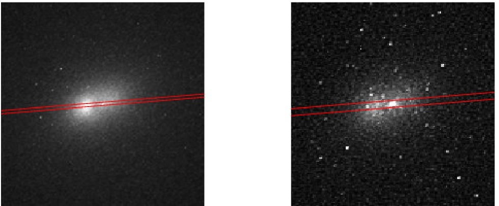
Figure 1.— STIS slit positions superimposed on the WFPC2 images from Lauer et al. (1998). The left panel shows the 0$\farcs$1 slit position for the Ca II spectrum on the F555W image, and the right panel shows the 0$\farcs$2 slit position for the blue spectrum on the F300W image. The images cover the central 6.4 arcsec by 6.4 arcsec. North is 55.7 degrees counter-clockwise from up.

Table 1STIS Instrument Configurations

Parameter	Red Spectrum	Blue Spectrum
Detector gain (e- per ADU)	1.0	1.0
Grating	G750M	G430L
Wavelength range	8272 Å $-$ 8845 Å	2900 Å $-$ 5700 Å
Reciprocal dispersion (Å pixel-1)	0.56	2.73
Slit width (arcsec)	0.1	0.2
Comparison line FWHM (pixel)	3.1	3.5
R $=\lambda/\Delta\lambda$	4930	450
Instrumental dispersion $\sigma_{\rm instr}$ (km s-1)	56	284
Scale along slit (arcsec  pixel-1)	0.051	0.051
Slit length (arcmin)	0.8	0.8
Integration time (sec)	20790	2040

3. Kinematics of the Double Nucleus P1 $+$ P2

The calcium triplet spectroscopy sees only the red giant stars that make up the double nucleus, P1 $+$ P2. It is blind to P3, which contributes essentially no light at $\lambda\simeq 8500$ Å. The kinematic properties of the red stars are illustrated in Figure 2.

In Figure 2, the spectrum of the bulge has been subtracted following procedures discussed in KB. Bulge subtraction is analogous to sky subtraction in the sense that it removes the effects of a contaminating spectrum that is not of present interest. As shown in KB, the bulge of M 31 dominates the light distribution only at radii $r$ ${}_{>}\atop{{}^{\sim}}$ 2^′′. At $r<1^{\prime\prime}$, it contributes about 20 % of the light. So over the radii of interest in Figure 2, bulge stars are a minor foreground and background contaminant; they do not significantly participate in the dynamics of the double nucleus. It is routine to estimate the small contribution of bulge stars to the STIS red spectrum and to subtract it. Figure 2 is therefore a pure measure of the kinematics of the stars that make up the double nucleus.

Figure 2 also shows the bulge-subtracted nuclear kinematics measured with the Canada-France-Hawaii Telescope (CFHT) (KB). Taking into account both the PSF and the slit, the effective Gaussian dispersion radius of the effective PSF was $\sigma_{*}=0$.^′′$297$ (Kormendy 2004). The corresponding resolution of the STIS red spectroscopy is $\sigma_{*}=0$.^′′$052$.

Confirming results of KB, the dispersion profile of the red stars reaches a sharp peak slightly on the anti-P1 side of P3. The peak dispersion is higher at STIS resolution ($\sigma=373\pm 50$ km s^-1) than at CFHT resolution ($\sigma=287\pm 9$ km s^-1). The rotation curve is also asymmetric; the maximum rotation velocity is larger on the anti-P1 side than it is in P1. Again, the asymmetry is larger and the radius of maximum rotation is smaller at STIS resolution than at CFHT resolution. These observations are consistent with and provide further evidence for Tremaine’s (1995) model for the double nucleus as an eccentric disk of stars orbiting the central BH. The Appendix provides more detailed discussion.

Panel 1 shows the double nucleus of M 31 rotated $\sim 185^{\circ}$ clockwise with respect to Figure 1. It is a $I$ $+$ $V$ $+$ 3000 Å composite from KB. P1 is brighter than P2 in red light. Embedded in P2 is P3, i. e., a tiny cluster of blue stars that is invisible in $I$ but brighter than P1 in the ultraviolet. The background image in Panel 2 is a similar $V$ $+$  3000 Å composite that better shows the small radius of P3. Panel 2 includes an $I$-band brightness cut along the P1 – P2 axis (lower curve) and a $V$-band cut through the blue cluster P3 (upper curve). The points are the brightness profile in the STIS spectrum; they are used to register the kinematics with the photometry in radius. Along the P1 – P2 axis, radius $r=0$ is chosen to be the center of P3 (note that in KB we centered the radius scale at $0\farcs 068$, not P3). Panels 3 and 4 show velocity dispersions and rotation velocities along the P1 – P2 axis after subtraction of the bulge. The ground-based points (crosses) are from the Subarcsecond Imaging Spectrograph (“SIS”) and the CFHT (KB). The STIS data (filled circles) are Fourier quotient reductions. Bacon et al. (2001) made an independent reduction of our red STIS spectrum; it is consistent with ours.

4. The Integrated Spectrum of P3

4.1. P3 is Made of A-Type Stars

P3, the compact blue cluster, is illustrated in the two panels of images in Figure 2. It is embedded in P2 but is not concentric with it; the photocenter of P2 is $\sim$ 0$\farcs$03 on the anti-P1 side of the blue cluster. The center of the bulge is slightly off in the opposite direction, i. e., toward P1 (see KB and discussion below). Note that we choose $r=0$ to be the center of P3, whereas KB chose $r=0$ to be the center of the bulge.

Linear intensity cuts through the blue and red spectra of P1 $+$ P2 $+$ P3. Each cut is an average over the wavelength range given in the key. The contrast between the blue cluster P3 and the underlying red nucleus P2 is largest at 4000 Å. It is smaller at redder wavelengths because the stars in P3 are blue. It is smaller at bluer wavelengths because the spectrum of P3 has a strong Balmer break (Figure 4). The two leftmost vertical dashed lines indicate the region in which the background spectrum was derived. The two rightmost vertical dashed lines indicate the radius range over which we averaged the background-subtracted P3 spectrum shown in Figures 4, 5 and 6.

We obtained our STIS spectrum at $\lambda\lambda\simeq 3500$ to 5000 Å in part to study this issue. Over the above wavelength range, P3 provides a strong signal, much stronger than that indicated by the $V$-band brightness cut in Figure 2. Figure 3 shows brightness cuts through the red and blue STIS spectra in various wavelength ranges. The blue cluster is essentially invisible at 8300 – 8800 Å in the red spectrum. We assume that this spectrum provides the surface brightness profile of the underlying double nucleus. With respect to this profile, P3 is, in general, more prominent at bluer wavelengths. The contrast over P1 $+$ P2 is highest at 3800 – 3950 Å. Then P3 gets less prominent at 3600 – 3750 Å; the reason turns out to be that the spectrum has a strong Balmer break (Figure 4). The important conclusion from Figure 3 is that the spectrum of P3 is almost as bright as the underlying spectrum of P1 $+$ P2 at just the wavelengths where hydrogen Balmer lines are strongest.

It is therefore possible to extract a clean spectrum of P3 despite the short integration time and modest signal-to-noise ratio. We averaged the spectrum of P3 over the 0$\farcs$2 = four spectral rows in which it is brightest (right pair of dashed lines in Figure 3). We approximated the spectrum of the underlying P2 stars by averaging 14 rows of the spectrum on the anti-P1 side of P3 (left pair of dashed lines in Figure 3.) The 8300 – 8800 Å brightness cut was used to scale this average P2 spectrum to the P2 brightness underlying P3. The result was subtracted from the four-row average spectrum of P2 $+$ P3. The resulting spectrum of P3 is shown in black in Figures 4 – 6.

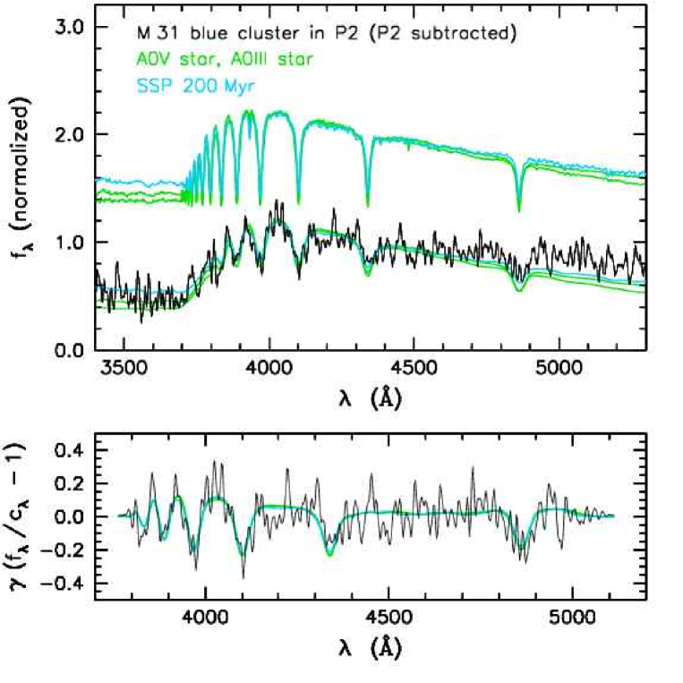
Figure 2.— Spectrum (black) of the central 0$\farcs$2 of the blue cluster P3. The superposed spectrum of the stars in the bulge and nucleus has been subtracted. Flux is in arbitrary linear units. In the lower panel, the spectrum has been divided by a polynomial $c_{\lambda}$ fitted to the continuum; it has been normalized to zero intensity, and multiplied by the mean ratio $\gamma$ of the line strength in the standard stars to that in P3. The colored lines show the spectra of an A0 dwarf star, an A0 giant star, and a Bruzual & Charlot (2003) starburst of age 200 Myr before (top) and after (overplotted on the data) broadening to the line-of sight velocity distribution that best fits the cluster spectrum. The fit was carried out with the Fourier correlation quotient program (Bender 1990).

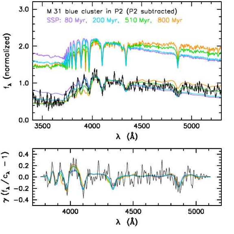
Figure 3.— This figure is analogous to Figure 4 except that the spectrum of the blue cluster P3 is compared with Bruzual & Charlot (2003) starbursts of various ages given in the key. The fit to the red continuum is best for an age of $\sim$ 510 Myr, but then the strengths of the Balmer lines H$n$ for $n\geq 5$ are wrong relative to the strengths of the redder lines. This problem gets worse for older starburst ages. Starbursts younger than 200 Myr are too blue; their Balmer breaks are too small to fit the observed spectrum.

The stellar population of P3 is dramatically different from that of P1 and P2. The spectrum in Figure 4 is dominated by Balmer absorption lines. At least five Balmer lines are visible, starting with H$\beta$ at $\lambda_{\rm obs}\simeq 4856$ Å. Also prominent is a strong Balmer break. In fact, the spectrum is very well matched by velocity-broadened spectra of A giant and dwarf stars. This confirms that the nucleus is made mostly of A-type stars as Lauer et al. (1998) and Brown et al. (1998) suggested.

4.2. The Remarkably High Velocity Dispersion of P3:
The Supermassive Black Hole Is In The Blue Cluster

The blue cluster has a remarkably high velocity dispersion. Using an A0 dwarf star from Le Borgne et al. (2003) as a template, the Fourier correlation quotient program (Bender 1990) gives a velocity dispersion of $\sigma=962\pm 105$ km s^-1. An A0 giant star gives $\sigma=984\pm 107$ km s^-1. A-type stars have intrinsically broad lines, but $\sigma$ is so large that the difference between using giants and dwarfs is insignificant. The above fits are illustrated in Figure 4. The match to the lines and to the Balmer break is excellent. The results are robust; plausible changes in the intensity scaling of the P2 spectrum that was subtracted produce no significant change in $\sigma$.

The best-fitting 200-Myr-old stellar population model (Figure 5, § 4.3) gives a dispersion of $\sigma=984\pm 106$ km s^-1. We adopt the average of the dispersion values given by the A dwarf star, the A giant star, and the 200-Myr-old stellar population model; this gives $\sigma=977\pm 106$ km s^-1 as our measure of the velocity dispersion of P3 integrated over the central 0$\farcs$02.

Despite its tiny size (half-power radius $\simeq 0\farcs 06\simeq 0.2$ pc; Lauer et al. 1998), P3 has the highest integrated velocity dispersion measured to date in any galaxy. The velocity dispersion of P3 is even larger than the line-of-sight velocity dispersion of the Sgr A* cluster in our Galaxy ($\sigma=498\pm 52$ km s^-1 to $840\pm 104$ km s^-1, depending on the sample of stars chosen, Schödel et al. 2003). The high velocity dispersion of P3 is especially remarkable in view of the observation (Figure 2) that the velocity dispersion of the red stars along the same line of sight is only $\sim 250$ km s^-1. The maximum velocity dispersion of P2, $373\pm 48$ km s^-1 at $\Delta r\simeq 0\farcs 06$ on the anti-P1 side of the blue cluster, is much smaller than that of P3. Even the remarkably high velocity dispersion, $\sigma=440\pm 70$ km s^-1 measured in P2 by Statler et al. (1999) is much smaller than the velocity dispersion of P3. This confirms the conclusion of KB that the M 31 supermassive black hole is in the blue cluster.

4.3. Fit of a Starburst Spectrum to P3

The overall continuum slope of P3 is best fitted not by a single A-type star but rather by the spectrum (Bruzual & Charlot 2003) of a single starburst population (SSP in Figures 4 and 5) of age $\sim 200\pm 50$ Myr and solar metallicity. The blue continuum fit is essentially perfect; the red continuum fit is improved slightly over the single star fits. Starburst spectra with a range of ages are shown in Figure 5. Using older starbursts allows us to fix the fit to the 5000-Å continuum, but only at an unacceptable price: the bluest Balmer lines are no longer well fitted. Complicating the model further would be overinterpretation; the error in the red continuum fit could be due to imperfect P2 subtraction or to small amounts of dust. But it is clear that we cannot exclude some admixture of older stars. Reasonable changes in metallicity also do not affect the fit: metallicity changes are largely degenerate with age changes.

Sample colour magnitude diagram of a 200 Myr old single burst population with solar metallicity and a total luminosity of $M_{V}=-5.7$. The spectrum is dominated by stars of $\sim$ 10000 K temperature. The diagram has been generated using the synthetic color-magnitude diagram algorithm of the Instituto de Astrofisica de Canarias (Aparicio & Gallart 2004).

How many stars make up P3? For an absolute visual magnitude of $M_{V}\approx-5.7$ (Lauer et al. 1998), we estimate the answer in Figure 6, using IAC-STAR, the synthetic color-magnitude diagram (CMD) algorithm of the Instituto de Astrofisica de Canarias (Aparicio & Gallart 2004). A 200-Myr-old, single-burst population of solar abundance implies that about 200 stars between spectral types A5 and B5 dominate the spectrum. The large number of stars at the same temperature of $\sim$ 10000 K explains why the spectrum of P3 is so similar to that of a single A0 star. Figure 6 also shows why P3 has a fairly smooth appearance, although surface brightness fluctuations are visible in Figure 8. Only a few red evolved stars are present, and they do not contribute significantly to the light of P3. Future observations with resolutions of about 0.01 arcsec should resolve the brightest stars close to the BH.

For a Salpeter (1955) initial mass function with a lower mass cut-off at 0.1 $M_{\odot}$, the total number of stars on the main sequence at present is $\sim$ 15000, their total mass is about 4200 solar masses. If the burst originally produced stars up to 100 $M_{\odot}$, then the initial total mass of P3 was $\sim$ 5200 $M_{\odot}$. Given the inefficiency of star formation, the total gas mass required to form P3 probably was of the order $10^{6}$ $M_{\odot}$.

Forming stars so close to a black hole is not trivial. It may be possible if $\sim 3\times 10^{6}{\thinspace}M_{\odot}$ of gas could be concentrated into a thin disk of radius 0.3 pc and velocity dispersion 10 km s^-1. Then Toomre’s (1964) stability parameter Q $\simeq$ 1. It is not easy to see how such an extreme configuration could be set up, especially without forming stars already at larger radii. Well before the black hole makes star formation difficult, the surface density of the dissipating and shrinking gas disk would get high enough so that the Schmidt (1959) law observed in nuclear starbursting disks (Kormendy & Kennicutt 2004, Figure 21) would imply a very high star formation rate. This star formation would have to be quenched until the gas disk got small enough to form P3. And then the star formation would have to be very inefficient to put only $\sim$ 5200 $M_{\odot}$ of the $\sim 3\times 10^{6}{\thinspace}M_{\odot}$ of gas into stars. Similar considerations make it difficult to understand young stars near the Galactic center black hole (e. g., Morris 1993; Genzel et al. 2003, Ghez et al. 2003, 2004). Nevertheless, young stars – or at least: high-luminosity, hot stars – are present. Complicated processes of star formation (e. g., Sanders 1998) may not realistically be evaluated by a simple argument based on the Toomre $Q$ instability parameter. So, if a dense enough and cold enough gas disk can be formed, star formation may be possible, even close to a supermassive black hole.

4.4. Could the Hot Stars in P3 Result From Stellar Collisions?

The alternative to a starburst could be that the hot stars of P3 are formed via collisions between lower mass stars in P3 or even in P1 $+$ P2. Yu (2003) argues that the collision timescales are too long to be of interest. It would be interesting to revisit this issue given the conclusion of § 6.1 that P3 is a cold stellar disk. In any case, it is worth noting that the conversion of (say) a high-mass, 0.5 $M_{\odot}$ main sequence star in P2 into an A star requires merging $\sim 6$ stars without mass loss. It is not easy to see how the A stars in P3 could originate by collisions.

Thus the situation in P3 is similar to that in our Galaxy. No explanation of the hot stars looks especially plausible.

4.5. P3 is Not Made of White Dwarf Stars

Finally, we need a sanity check to make sure that we are not completely misinterpreting the observations. Dynamically, we detect a $10^{8}$-$M_{\odot}$ central dark object. This is associated with a tiny and faint nucleus comprised of hot stars that have extraordinarily broad absorption lines. White dwarf stars have extraordinarily broad absorption lines. If they are not too old, they can easily have an A-type spectrum, and if they are not too young, they can easily contribute mass without contributing much light. It is natural to wonder – could P3 be a cluster of white dwarfs? Could they simultaneously explain the broad-lined, A-type spectrum and the central dark mass? This possibility is not excluded by stellar collision or cluster evaporation timescales (Maoz 1995, 1998).

Figures 7 and 8 show that P3 cannot be made of white dwarfs. Figure 7 compares the spectrum of P3 with that of a typical DA white dwarf observed in the Sloan Digital Sky Survey (SDSS). The star was chosen to have Balmer line strengths comparable to those in P3. It is approximately the best match to P3 that can be achieved with white dwarf spectra. Its lines are narrower than those of P3, so we can fit the observed line widths (bottom panel of Figure 7) with $\sigma=885\pm 126$ km s^-1. That is, this relatively narrow-lined white dwarf gives a dispersion similar to those implied by main sequence and giant A stars. The fit to the line widths is less good than the fit provided by A0 V stars, but it is not inconsistent with our low $S/N$ spectrum of P3. If we had only the spectrum of this white dwarf as observed over the relatively narrow wavelength region redward of the Balmer break, we could not exclude white dwarf stars.

However, the continua of white dwarf stars do not fit the large Balmer break in P3. SDSS J094624.30$+$581445.4 (Figure 7) does not show this – it and most other white dwarfs have not been observed at blue enough wavelengths to reach the Balmer break. Therefore we resort to model spectra kindly provided by Detlev Koester (Finley, Koester and Basri 1997; Koester et al. 2001). Figure 7 shows a model spectrum that has line profiles similar to those in the observed white dwarf. The price of having narrow enough lines to fit the absorption lines in P3 is that there is essentially no Balmer break. Such a star cannot fit the continuum of P3. This result is very robust; it is not affected by uncertainities in the subtraction of the spectra of P1 $+$ P2.

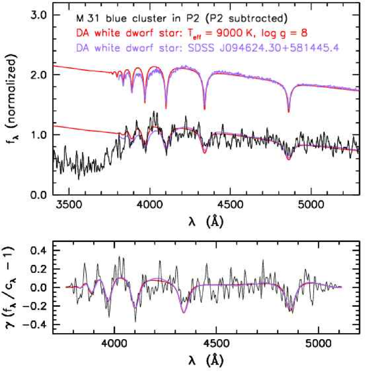
Figure 4.— Spectrum of P3 fitted with approximately matched observed and model white dwarf spectra. The observed spectrum is from the SDSS (Kleinman et al. 2004; see http://www.sdss.org). The model spectra used in Figures 7 and 8 are from Finley, Koester, & Basri (1997) and from Koester et al. (2001). The fits of white dwarf spectra to P3 are significantly worse than the ones in Figures 4 and 5. The absorption lines of the white dwarfs are intrinsically too strong, and the white dwarfs fail completely to fit the large Balmer continuum break in the P3 spectrum. However, the implied velocity dispersion, $\sigma=885\pm 126$ km s^-1, is consistent with our adopted value, $\sigma=977\pm 106$ km s^-1.

Choosing different white dwarf parameters does not solve this problem. No combination of temperature and gravity allows a simultaneous match to the Balmer line strengths and the Balmer break. Figure 8 shows fits of model white dwarf spectra with temperatures $T=7000$ K, 8000 K, 10000 K, and 12000 K, respectively. For each temperature, we try surface gravities of $10^{7}$, $10^{8}$, and 10⁹ cm s^-2.

Temperature $T\simeq 7000$ K is too cold. The stellar lines are too weak. Not surprisingly, these stars have no Balmer break at all. Despite the bad continuum fit, the narrow lines in the white dwarf templates give dispersions, $\sigma=945\pm 103$ km s^-1, $\sigma=987\pm 107$ km s^-1, and $\sigma=1063\pm 115$ km s^-1, that are consistent with our adopted result.

At $T=8000$ K, the fit to the lines is better, although not as good as for A0  dwarf or giant stars. The dispersion remains high ($\sigma=930\pm 101$ km s^-1, $\sigma=929\pm 101$ km s^-1, and $\sigma=952\pm 103$ km s^-1). Again, the Balmer break in the white dwarfs is too weak.

At $T=10000$ K, the stellar lines are much broader. The fit to P3 is acceptable after scaling the line strengths. For $\log{g}=7$, 8, and 9, $\sigma=784\pm 120$ km s^-1, $769\pm 134$ km s^-1, and $821\pm 150$ km s^-1, respectively. Note that without line-strength scaling, the broadened white dwarf spectrum does not fit the galaxy. And, even though the lines are now strong enough when $\log{g}$ is large to produce a Balmer break, it is still too small to fit the spectrum of P3. The green line emphasizes how much an A0 V star fits the spectrum of P3 better than does any white dwarf.

Increasing the temperature further is counterproductive. At $T=12000$ K, the lines are too strong and too broad to fit P3, although we still obtain high dispersions ($\sigma=705\pm 144$ km s^-1, $\sigma=676\pm 166$ km s^-1, and $\sigma=680\pm 190$ km s^-1). Even high temperatures do not produce strong enough Balmer breaks.

We conclude that no spectral synthesis of white dwarf stars of different temperatures or gravities would fit P3. The ones that fail least badly – those that fit the lines but not the Balmer break – imply velocity dispersions that are consistent with values derived from A0 dwarf or giant stars.

For a compact cluster of white dwarfs to be a viable alternative to a supermassive black hole, it must be dark. That is, it must be old. We explore this option further in Section § 8.

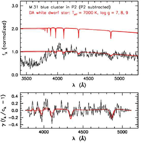
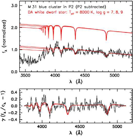
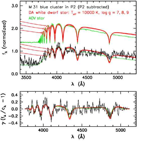
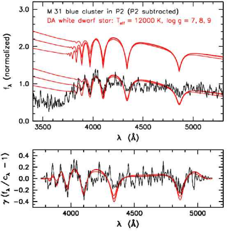
Figure 5.— Fits to the spectrum of P3 (black) of model white dwarf spectra (red) with temperature $T_{\rm eff}=7000$ K, 8000 K, 10000 K, and 12000 K (see the key). At each temperature, surface gravities of $g=10^{7}$, $10^{8}$, and $10^{9}$ cm s^-2 are used. The green line shows the fit of an A0 dwarf star. Compare Figure 6.

5. Light Distribution of P3

For a dynamical analysis of P3 (§ 6), we need its light distribution with P1 $+$ P2 subtracted. To derive this, we scaled the HST F555W image to the HST F300W image such that P1 disappeared after subtraction. The resulting image of P3 is shown in Figure 9. We then fitted P3 with Sérsic (1968) models,

$$I(r)=I_{0}\exp[-(r/r_{0})^{1/n}]~{},$$

convolved with the HST point spread function as in Lauer et al. (1998). The PSF was constructed from two exposures of the

standard star GRW+70D5824 (u2tx010at, u2tx020at). The free parameters in the fit were central surface brightness $SB_{0}$, scale length $r_{0}=\sqrt{a_{0}b_{0}}$ ($a$, $b$ = semimajor, semiminor axis), Sérsic $n$, position angle $P.A.$, ellipticity $1-b/a$, and center coordinates. Individual faint point-like sources in the outskirts of P3 were masked before fitting. The best fit over the radius range $r<0\farcs 3$ was obtained for Sérsic index $n=1$, major-axis scale length $a_{0}=0\farcs 1\pm 0\farcs 01$, PSF-convolved ellipticity $1-b/a=0.33\pm 0.03$, and position angle $P.A.=63^{\circ}\pm 2^{\circ}$ (this is 119^∘ counterclockwise from vertical in Figure 9).

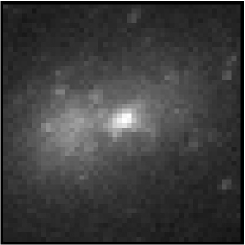
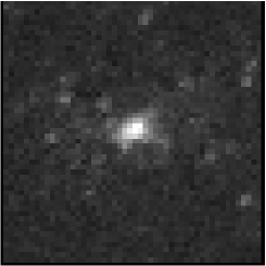
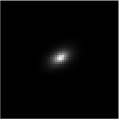
Figure 6.— Left to right: (i) F300W image of the blue nucleus, P3, superposed on nuclei P1 and P2; (ii) F300W image of P3 after subtraction of the F555W image intensity-scaled to the F300W image in (i); (iii) PSF-convolved inclined disk model for P3; and (iv) difference between images (ii) and (iii) showing the quality of the model and the residual surface brightness fluctuations. All images are 2$\farcs$5 by 2$\farcs$5. North is 55.7 degrees counter-clockwise from up, as in Figure 1.

Observed radial profiles (red) of P3 surface brightness SB, ellipticity $1-b/a$, and position angle PA versus semi-major axis $a$. Lucy-deconvolved profiles are shown in green. The HST PSF is shown in light blue (with arbtitrary zeropoint). The inclined disk model before and after convolution with the HST PSF is represented by blue and black lines, respectively. The observed profiles are over-sampled – neighboring points are not independent.

Table 2

Parameters of the thin disk model of P3

Parameter${}^{)}_{)}$	Value
$m_{\rm F300W}$	$18.6\pm 0.1$
$M_{\rm F300W}$	$-5.8\pm 0.1$
Sérsic $n$	1
exp. scale length $a_{0}$	$0\farcs 1\pm 0\farcs 01$
$SB_{0,{\rm F300W}}$ (face-on)	$15.6\pm 0.1$ mag arcsec-2
inclination	$55^{\circ}\pm 2^{\circ}$
position angle	$63^{\circ}\pm 2^{\circ}$

The three color images at the top show the PSF-broadened thin disk model of P3. The images cover $0\farcs 5\times 0\farcs 5$. Shown from left to right are: (i) P3 surface brightness; intensities range from 0 (black) to 1 (white); (ii) P3 rotation velocity field with the slit and radial bins superposed; the velocity amplitudes range from $-700$ km s^-1 (black) to $+700$ km s^-1 (white); (iii) P3 velocity dispersion, ranging from 150 km s^-1 (black) to 1000 km s^-1 (white). The panels of plotted data points show the P3 radial profiles (red) of rotation velocity (bottom) and velocity dispersion (middle), folded around P3’s center. Open and closed symbols are from opposite sides of the center. The sense of rotation is the same as for the eccentric disk P1 + P2. The top plot shows the best-fitting Keplerian circular velocity curve as a dashed line. It implies a black hole mass of $\sim 1.4\times 10^{8}$ $M_{\odot}$. Convolving the circular velocity field with the PSF and integrating it over the pixel size and slit width yields the model rotation and dispersion profiles shown as dotted curves in the bottom and the middle panels.

The PSF-convolved model and the difference between P3 and the model are illustrated in Figure 9. We also compare model and P3 with respect to their isophotal parameters. Figure 10 shows the surface brightness, ellipticity and position angle profiles of the observed P3, the model and the PSF-convolved model. Also shown are deconvolved P3 profiles, which were obtained from 15 iterations with the Richardson-Lucy deconvolution algorithm implemented in the ESO MIDAS package. The deconvolved surface brightness profile obtained here agrees well in shape with the one by Lauer et al. (1998). Figure 10 shows that the model represents P3 reasonably well, especially over the radius range for which we can analyse the kinematics (§ 6). Surface brightness fluctuations become large at radii beyond 0$\farcs$25. Still, the model is adequate out to $\sim$ 0$\farcs$4.

If P3 is an inclined, thin disk, then the observed ellipticity implies an inclination $i=55^{\circ}\pm 2^{\circ}$. This is compatible with the inclination of the eccentric disk P1 $+$ P2: Peiris & Tremaine (2003) derive $i=54^{\circ}$, and Bacon et al. (2001) get $i=55^{\circ}$. The model parameters of P3 are summarized in Table 2. Whether P3 really is a thin disk can only be checked with kinematical data. We discuss these in the next section.

6. Dynamics of P3

Figure 11 shows the rotation velocity and velocity dispersion profiles of P3. Table 3 lists the data. We used FCQ for the analysis but did not fit the $h_{3}$ and $h_{4}$ Gauss-Hermite parameters because the S/N of the data is only $\sim 3$ per Å. Outside of the central pixel, P3 rotates rapidly, with an observed amplitude of $573\pm 61$ km s^-1 (weighted mean of all points with $|r|>0\farcs 01$). P3 rotates in the same sense as P1 $+$ P2. The apparent velocity dispersion drops from $\sim$ 1200 km s^-1 in the central pixel to $<$ 500 km s^-1 at $r=0\farcs 15$ = 0.55 pc. These values are consistent with the velocities seen in the extreme wings of the line-of-sight velocity distribution of the red stars at $r\sim-0\farcs 1$ (see Appendix). The kinematic data securely locate the BH at the center of P3 with an uncertainty of about 1/3 of a pixel $=0\farcs 02=0.07$ pc.

Table 3

Kinematics of P3

radius	V	$\Delta$V	$\sigma$	$\Delta\sigma$
arcsec	km s-1	km s-1	km s-1	km s-1
$-0.16$	$525$	197	237	233
$-0.11$	$616$	144	337	170
$-0.06$	$582$	111	583	131
$-0.01$	$170$	169	1183	200
$+0.04$	$-659$	117	777	139
$+0.09$	$-387$	179	769	211
$+0.14$	$-420$	273	505	322

We wish to combine the surface brightness data (Table 2) and the kinematic data (Table 3) to make dynamical models. Because the pixel size, slit width, and PSF are all similar to the size of P3, unresolved rotation must contribute to the apparent velocity dispersion. Actually, almost all of the light of P3 falls into the slit. Despite this and despite the modest apparent flattening, P3’s apparent rotation velocity and velocity dispersion are similar. Therefore, it is reasonable to expect that P3 is an intrinsically flat object with $V\gg\sigma$.

For these reasons, we first model P3 as a flat disk with an exponential profile and an inclination $i\sim 55^{\circ}$ (§ 6.1). Then (§ 6.2), we explore more nearly edge-on models in which P3 has some intrinsic thickness.

6.1. P3 as a Flat Exponential Disk

We construct a dynamical model in which we assume that P3 is a flat disk with the parameters in Table 2 and a negligible instrinsic velocity dispersion. The BH affects the structure of the galaxy interior to $r_{\rm cusp}\simeq GM_{\bullet}/\sigma^{2}=5\farcs 6\thinspace[M_{\bullet}/(10^{8}{\thinspace}M_{\odot})]$, where $G$ is the gravitational constant and $\sigma=145$ km s^-1 (Kormendy 1988) is the velocity dispersion of the bulge just outside the region affected by the BH. Since P3 is tiny compared to $r_{\rm cusp}$, the black hole dominates the gravitational potential. The distribution of the stars is completely constrained by the photometry, so the only free parameter is the BH mass. To compare the model with the observed rotation and velocity dispersion profiles, we convolve the Keplerian velocity field with the PSF and integrate it over the 0$\farcs$2 slit width and 0$\farcs$05 CCD pixels (see Figure 11, top-middle panel). This is done with small subpixels to obtain smooth profiles of rotation velocity and velocity dispersion.

Figure 11 shows the results. The observed rotation and dispersion profiles (open and closed symbols) are well matched by the model (dotted curves). Estimating the mass of the black hole is straightforward, because $M_{\bullet}$ is the only free parameter. The best fit gives $M_{\bullet}=(1.4\pm 0.2)\times 10^{8}$ M_⊙. The reduced $\chi^{2}_{n}$ is $\sim$ 1 (Figure 12).

The BH mass derived with the thin disk model does not depend significantly on inclination over the range allowed by the photometry ($\pm 2^{\circ}$). Changing the inclination away from the best value increases $V$ and decreases $\sigma$ or vice versa. Then $\chi^{2}$ increases slightly, but the shape of the $\chi^{2}$ distribution as a function of black hole mass does not change significantly. We also varied the scale length of the P3 disk, its total luminosity, and its position angle on the sky within the errors. There was no significant effect on $M_{\bullet}$. The total luminosity and mass of P3 are irrelevant provided that the BH dominates the potential. The position angle would have to be changed well beyond its estimated errors to achieve a visible effect on the velocities. Changing the radial scale length redistributes light and makes the rotation and dispersion profiles flatter or steeper. Within the errors, $M_{\bullet}$ is not affected.

The circular velocities for the thin disk model are shown in the top panel of Figure 11. Future observations that resolve individual stars should see velocities of 1000 to 2000 km s^-1. Such measurements can also test how much the observed velocities and dispersions are affected by shot noise due to the small number of stars in P3. Checking how close to circular the disk really is will also be important.

If P3 is a thin stellar disk, can it be stable? The answer is yes, as long as its stellar mass is not very much larger than 5200 $M_{\odot}$. Even relatively small dispersions will not lead to significant two-body relaxation. Using Equation 8-71 in Binney & Tremaine (1987), we obtain relaxation times of the order of a Hubble time. Moreover, the critical velocity dispersion for local stability (Toomre 1964) is small, $\sigma_{\rm crit}\ll 1$ km s^-1. This is a consequence of the fact that the potential is dominated by the black hole. That is, the P3 disk is dynamically analogous to Saturn’s rings rather than to a self-gravitating disk. Therefore, if earlier starbursts contributed mass without affecting its present spectrum, the P3 stellar disk is likely to be locally stable and immune from two-body relaxation. And if P3 consists only of young stars, then it has not had time for significant dynamical evolution.

6.2. P3 Schwarzschild Models

To investigate the effect on $M_{\bullet}$ of allowing P3 to have some thickness in the axial direction $z$ and therefore to be more nearly edge-on than $i=55^{\circ}$, we fitted Schwarzschild (1979) models to the photometric and kinematic data. We used the regularized maximum entropy method as implemented by Gebhardt et al. (2000a, 2003) and by Thomas et al. (2004). The program was constrained to reproduce the observed surface brightness distribution of P3. We considered three inclinations $i=58^{\circ}$, $66^{\circ}$, and $90^{\circ}$, corresponding to intrinsic axial ratios of P3 of $0.26$, $0.44$, and $0.57$, respectively. Black hole masses were varied until the kinematic data were reproduced as well as possible, as indicated by the $\chi^{2}$ values in Figure 12.

In the Schwarzschild code, phase space is quantized on a polar grid that is not optimized for closed orbits. It is therefore helpful if the orbits are not quite closed. For this reason, we did not use a point mass for the central dark object but rather used a Plummer sphere with a half-mass radius $r_{h}=0\farcs 01$. Given the spatial resolution of the data, this is essentially equivalent to a black hole (see Figure 14).

Models that put significant weight on entropy maximization did not fit the kinematics. They rotated too slowly, because they contained retrograde orbits. This is expected, because entropy maximization is not appropriate for highly flattened systems with strong rotational support.

Switching off the entropy maximization (this corresponds to a high regularization parameter in Thomas et al. 2004) results in better fits. Figure 12 shows $\chi^{2}$ values as a function of inclination and dark mass $M_{\bullet}$. We conclude that the lowest inclination, $i=58^{\circ}$, is preferred, by $\Delta\chi^{2}\approx 2$ relative to the $i=66^{\circ}$ model and with higher significance relative to the more inclined models.

Rotation velocity and velocity dispersion profiles for the lowest-$\chi^{2}$ model at each inclination are shown in Figure 13. Reassuringly, the $i=58^{\circ}$ Schwarzschild model most nearly resembles the $i=55^{\circ}$ thin disk model. The fits then become progressively more different – and less good – as the models are made more edge-on.

Higher inclinations require higher BH masses. The reason is that, at higher inclinations, line-of-sight integration through the nearly edge-on, thick disk includes stars at relatively large radii that move mostly across, not along, the line of sight. They reduce the velocity moments and consequently require higher $M_{\bullet}$ to match the observed rotation velocities. The preferred black hole mass for the $i=58^{\circ}$ and $i=66^{\circ}$ Schwarzschild models is $\sim 2\times 10^{8}$ $M_{\odot}$. The highest black hole mass that is consistent with the data to within $\sim 1\sigma$ is given by the $i=58^{\circ}$ Schwarzschild model and is $\sim 2.3\times 10^{8}$ $M_{\odot}$ (Figure 12). The lowest black hole mass implied by the dynamics of P3 is given by the thin disk, $i=55^{\circ}$ model and is $\sim 1.2\times 10^{8}$ $M_{\odot}$ (§ 6.1).

It is instructive to examine the $i=58^{\circ}$ Schwarzschild model in more detail. Figure 14 shows its velocity moments. Rotation dominates the dynamics; $V_{\phi}$ is $\lesssim$ 20 % smaller than the circular velocity. At radii $r\gtrsim 0\farcs 1$, the model is approximately isotropic. To provide the thickness that is necessitated by the inclination $i>55^{\circ}$, $\sigma_{z}$ then increases substantially inward, although it remains smaller than the rotation velocity. The difference between the adopted Plummer model and a central point mass is small except for the innermost data point.

$\chi^{2}$ profiles for models of P3. The black lines refer to the thin disk model with inclination $55^{\circ}$, the coloured lines show three Schwarzschild models with inclinations $58^{\circ}$, $66^{\circ}$, and $90^{\circ}$. The dashed lines assume that the massive dark object is a Plummer sphere with radius $0\farcs 01$, the full black line assumes a black hole.

Rotation velocities and velocity dispersions of P3 as in Figure 11 (red open and closed symbols). Overplotted as colored dashed lines are three Schwarschild models with different inclinations and black hole masses. The thin disk model of Figure 11 is shown as a dotted black line.

Major-axis velocity moments of the best $i=58^{\circ}$ Schwarzschild model for P3, corresponding to $M_{\bullet}=2\times\kern-2.0pt10^{8}$ $M_{\odot}$. The MDO is a Plummer sphere with half-mass radius $r_{h}=0\farcs 01$; its circular velocity is shown as a solid black line. A BH of the same mass would produce the Keplerian circular velocities indicated by the dashed curve.

Orbit structure of the Schwarzschild model with $i=58^{\circ}$, Plummer model dark mass $M_{\bullet}=2\times 10^{8}$ $M_{\odot}$, and half-mass radius $r_{h}=0\farcs 01$. For each orbit, the orbit weight $w_{i}$ per phase space volume is shown as a function of the $z$ component of its angular momentum $L_{z}$ normalized by the angular momentum $L_{c}$ of the circular orbit that has the same energy. In this figure only, $r$ is the average of the pericenter and apocenter radii of the orbit. Note that at all radii, only prograde orbits are significantly populated.

Figure 15 shows the corresponding orbit structure. As expected for a Schwarzschild model that is not too different from the thin disk model, retrograde orbits are strongly suppressed. However, as indicated by Figure 14, noncircular orbits get significant weight in order to produce that axial ratio $b/a\simeq 0.26$. As expected, this happens more near the center than at larger radii. However, nearly circular orbits dominate; otherwise $V_{\phi}$ would not be almost equal to $V_{c}$ in Figure 14.

6.3. Summary: Comparison of P3 and P1 $+$ P2

We conclude that the triple nucleus of M31 is made of two nested, disk-like systems. The P1 $+$ P2 disk is elliptical, has a radius of about 8 pc, and consists of old, metal-rich stars. If it is thin, it has an inclination of $\sim 54^{\circ}$ and a major-axis position angle of $\sim 43^{\circ}$ (Peiris & Tremaine 2003). The P3 disk is approximately circular and has a radius of about 0.8 pc. If it is thin, P3 has an inclination $i\sim 55^{\circ}$ that is the same as that of P1 $+$ P2. P3’s major-axis position angle at $r\leq 0\farcs 25$ is $\sim$ $63^{\circ}\pm 2^{\circ}$. That is, the inner P3 disk is slightly tilted with respect to the P1 $+$ P2 disk but is relatively close to the kinematical major axis, P.A.$\sim 56^{\circ}$, found by Bacon et al. (2001). At $r>0\farcs 25$, the major axis of P3 twists to $\sim 40^{\circ}$, essentially the position angle of P1 $+$ P2. The nested disks rotate in the same sense and have almost parallel angular momentum vectors.

7. The Mass of the Central Dark Object

We have demonstrated that disk-like models for P3 fit both the photometry and the kinematics of P3 exceedingly well. This allowed an estimate of $M_{\bullet}$ that is independent of all previous determinations. Besides black hole mass, only inclination is a free parameter in the fit to the rotation curve and the dispersion profile (Figures 11, 13).

Could systematic effects cause additional errors that are not included in the statistical errors, especially toward low BH masses? We mentioned in the previous section that some clumpiness in the distribution of stars could be hidden by PSF blurring and may affect the measured velocities and dispersions. We carried out a simple check for this effect by fitting subsamples of data points. E.g., a fit to just the innermost three points in Figure 11 typically yields BH masses about 15% higher, while omitting these three points results in 25% lower masses. All values obtained in this way fell in the range allowed by the $\chi^{2}$-profiles in Figure 12, so this effect does not seem to be very important.

Some non-circularity of the P3 disk could be hidden as well. P3 could contain stars on elongated orbits that have their pericenters within the range of the kinematic data (0$\farcs$15) but apocenters spread out over radii well beyond this radius. Figure 9 shows faint blue stars that could be such objects. This would imply that P3’s velocity amplitudes are increased by rotation velocities that are faster than circular. It is difficult to estimate the size of this effect, but pericenter velocities of very radial stars can be at most a factor of 2 larger than pericenter velocities of stars on nearly circular orbits. Averaging over a set of orbits will reduce this number considerably. And if we wanted to fully exploit this effect, many more stars of P3 would have to be found outside of $\sim 0\farcs 18$ than inside, which is in contradiction with the observations. The Schwarzschild models also show that this trick does not work well. More radially biased models (obtained with higher entropy weighting and not shown here) require larger BH masses. Finally, if P3 originated in a star-forming gas disk, it could not contain nearly radial orbits, and we noted above that subsequent internal evolution of the P3 disk should be slow.

So, very special circumstances would be required to decrease $M_{\bullet}$ below $1\times 10^{8}$ $M_{\odot}$. On the high mass end, the black hole mass grows with increasing inclination of the model. However, the $\chi^{2}$ values become inacceptably large for inclinations above $\sim 60^{\circ}$ and, therefore, it is unlikely that the black hole mass is significantly larger than $\sim 3\times 10^{8}M_{\odot}$. Viable models for P3 are found in the inclination range $55^{\circ}<i<58^{\circ}$ and in the BH mass range $1.1\times 10^{8}M_{\odot}<M_{\bullet}<2.3\times 10^{8}M_{\odot}$. The upper limit takes into account that the Schwarzschild models were calculated assuming an MDO with $r_{h}=0\farcs 01$ and not a BH; the upper limit for a BH is $\approx 0.2\times 10^{8}M_{\odot}$ lower than for an MDO with $r_{h}=0\farcs 01$. The best fit and at the same time lowest black hole mass of $M_{\bullet}=1.4\times 10^{8}M_{\odot}$ is obtained for the thin disk model. This model is also preferred on astrophysical grounds, if P3 formed out of a thin gaseous disk. Therefore, our best estimate for the mass of the supermassive black hole in M 31 is $M_{\bullet}=1.4^{+0.9}_{-0.3}\times 10^{8}M_{\odot}$.

How does this compare with previous results? The black hole mass has now been estimated by five, largely independent techniques, (i) standard dynamical modeling that ignores asymmetries, (ii) the KB center-of-mass argument that depends on the asymmetry of P1 $+$ P2, (iii) the Peiris & Tremaine nuclear disk model that explains the asymmetry of P1 $+$ P2, (iv) full dynamical modeling that takes into account the self-gravity of the P1 $+$ P2 disk (Salow & Statler 2004), and (v) dynamical modeling of the blue nucleus P3, which is independent of P1 $+$ P2. The good news is that all methods require a dark mass with high significance. The bad news is that some of the results differ by more than two standard errors. In particular, the disagreement between the KB center-of-mass argument and the P3 models presented here is a concern. We therefore revisit the KB derivation in the subsection below. The models that best fit both the photometry and the kinematics – the Peiris & Tremaine (2003) eccentric disk model of P1 $+$ P2 and our thin disk model of P3 – agree within the errors and favor a high black hole mass of $M_{\bullet}\sim 1\times 10^{8}$ $M_{\odot}$. We also note that a higher black hole mass can be accommodated more easily in almost all models than a lower black hole mass.

The mass of the M 31 BH derived here is a factor of $\sim$ 2.5 above the ridge line of the correlation between $M_{\bullet}$ and bulge velocity dispersion $\sigma_{\rm bulge}$ (Ferrarese & Merritt 2000; Gebhardt et al. 2000b). Using the Tremaine et al. (2002) derivation,

$$\log\left(\frac{M_{\bullet}}{M_{\odot}}\right)\;=\;8.13\;+\;4.02\,\log\left(\frac{\sigma_{\rm bulge}}{200~{}\rm{km\ s}^{-1}}\right)~{},$$

$\sigma_{\rm bulge}\simeq 160$ km s^-1 implies that $M_{\bullet}\simeq 5.5\times 10^{7}$ $M_{\odot}$. We derive $M_{\bullet}=1.4^{+0.9}_{-0.3}\times 10^{8}$ $M_{\odot}$. Tremaine et al. (2002) already found significant scatter in the $M_{\bullet}-\sigma_{\rm bulge}$ relation at low masses. With the increased BH mass for M 31, scatter has become even more prominent. Considering, in addition to M 31, only the two closest other supermassive BHs, i.e. M 32 and the Galaxy, we get the following. M 32 has $\sigma_{\rm bulge}\sim 75$ km s^-1, a predicted $M_{\bullet}=2.6\times 10^{6}$ $M_{\odot}$ and an observed $M_{\bullet}=(2.9\pm 0.6)\times 10^{6}M_{\odot}$ (Verolme et al. 2002 corrected to distance 0.81 Mpc from Tonry et al. 2001). Our Galaxy has $\sigma_{\rm bulge}\sim 103$ km s^-1, a predicted $M_{\bullet}=9.4\times 10^{6}$ $M_{\odot}$ and an observed $M_{\bullet}=(3.7\pm 0.2)\times 10^{6}$ $M_{\odot}$ (Ghez et al. 2004). So M 31, M 32, and our Galaxy have black hole masses that are 2.5 times larger than, consistent with, and 3 times smaller than the ridge line of the $M_{\bullet}-\sigma_{\rm bulge}$ relation, respectively. This is strong indication for significant intrinsic scatter in the $M_{\bullet}-\sigma_{\rm bulge}$ relation, at least at the low-mass end.

7.1. Black Hole Mass From The Center-of-Mass Argument:
Kormendy & Bender (1999) Revisited

KB estimated that the center of P3 (blue dot in our Figure 16) is offset from the bulge center (horizontal dashed line) by about 0$\farcs$06. They then assumed that the central dark object is in P3 and estimated its mass based on the assumption that the combined system, BH $+$ P1 $+$ P2 $+$ P3, is in dynamical equilibrium. That is, they assumed that the center of mass of BH $+$ P1 $+$ P2 $+$ P3 is at the center of the bulge. Then $M_{\bullet}$ is inversely proportional to its distance from the bulge center and, if the mass of P3 is negligible, $M_{\bullet}$ is proportional to the mass of P1 $+$ P2. The latter was given by the light distribution and the measured mass-to-light ratio $M/L_{V}=5.7$. The resulting black hole mass was $M_{\bullet}\simeq(3.3\pm 1.5)\times 10^{7}$ M_⊙. This is at the low end of the range of published values and a factor of $\sim$ 4 smaller than the value derived here. As the stellar $M/L_{V}$ can hardly be a factor 4 larger, two explanations are possible for the discrepant BH masses: (i) P3 and the BH are a factor of 4 closer to the bulge center than KB derived, or (ii) the BH $+$ P1 $+$ P2 $+$ P3 system is not in equilibrium with respect to the bulge center.

We believe that the observations can be consistent with equilibrium and that the distance of P3 to the bulge center was overestimated by KB for the following reasons.

From KB, isophote center coordinates $X$ along the line joining P1 and P2 as a function of isophote major-axis radius $a$. A $V$-band HST WFPC2 image was measured twice, once masking out P2 (green) to measure the convergence of the P1 isophotes on the center of P1 (green dot) and once masking out P1 (blue) to measure the convergence of the P2 $+$ P3 isophotes on the center of P3 (blue dot). The brown and red points are measurements of individual isophotes in $H$- and $K^{\thinspace\prime}$-band images. The positions of the velocity center and of the center of mass of the BH and nucleus (if $M_{\bullet}=3\times 10^{7}$ $M_{\odot}$), each with error bars, are shown by the symbols labeled “V=0” and “COM”. The dashed line at $X=0$ marks the center position of the bulge that was adopted by KB. It was estimated by averaging all isophote center coordinates at $2\farcs 9<a<25\farcs 0$ ($1.3<a^{1/4}<2.24$). However, if $M_{\bullet}=1.4\times 10^{8}$ $M_{\odot}$, then the BH’s radius of influence is $r_{\rm cusp}\simeq 7\farcs 2$. Therefore KB estimated the bulge center position partly from isophotes that are at $a<r_{\rm cusp}$. Within this radius, the BH dominates the potential and isophotes do not need to be concentric to be in equilibrium (witness the eccentric disk). Since we now believe that the BH mass is large, we should derive the bulge center from correspondingly larger radii. The solid line is a least-squares fit to the bulge $X_{\rm center}$ values at $a>r_{\rm cusp}$. It shows that the isophote centers at the largest radii in the figure are approximately at the $X$ coordinate of P3. Therefore the BH is close to the luminosity-weighted center of the bulge.

Figure 16 revisits the center of mass argument. It is reproduced from KB and shows their estimate of the position of the center of the bulge as the dashed line at $X=0$. The isophote center coordinate $X$ is measured along the line joining P1 and P2. A conclusion about the position of the center of the bulge depends on the radius range chosen in which to average isophote $X$ values. KB calculated the average at $2\farcs 9<a<25\farcs 0$. A larger radius range was not possible because of the small size of the high-resolution images used. If $M_{\bullet}\sim 3\times 10^{7}$ $M_{\odot}$, then the above radius range is no problem – it is beyond the radii affected by the BH. However, if $M_{\bullet}$ is as big as $1.4\times 10^{8}$ $M_{\odot}$, then $r_{\rm cusp}\simeq 7\farcs 2$ and it is necessary to calculate the mean bulge $X$ at larger radii.

If we calculate the bulge center outside of $r_{\rm cusp}\simeq 7\farcs 2$, we obtain a mean $X$ position of $-0\farcs 033$ in Figure 16, i. e., half way between the KB bulge center and P3. Note that, unlike KB, we do not limit the averaging to points with $a<25\farcs 0$ but now also include two further points that we extracted from the QUIRC $H$-band image beyond this radius. In addition, we omit all center coordinates with errors larger than $0\farcs 2$.

A least-squares fit to the points with $a>7\farcs 2$ gives the short black line in Figure 16. It shows that the bulge isophote centers drift with increasing radius toward the $X$ position of P3. So the luminosity-weighted center of the bulge is close to P3.

This discussion suggests that the determination of the bulge center is less reliable than KB assumed. There are three reasons: (i) the BH sphere of influence is much larger than KB assumed, (ii) the bulge isophote centers drift toward P3 with increasing radius beyond $a$ = 2$\farcs$9, and (iii) the isophote centers oscillate – or at least, fluctuate – with radius because of dust or surface brightness fluctuations or perhaps a physical effect that we have not identified. If the BH is much more massive than P1 $+$ P2, then it is so close to the center of mass that $M_{\bullet}$ cannot be determined accurately from the COM argument.

The important conclusion, however, is that the observations of M 31 are consistent with dynamical equilibrium and with a large BH mass of $M_{\bullet}=1.4\times 10^{8}$ $M_{\odot}$.

8. Astrophysical Constraints on a Massive Dark Object Made of Dark Stars

Central dark masses are detected dynamically in 38 galaxies (see Kormendy & Gebhardt 2001; Kormendy 2004 for reviews). They are commonly assumed to be supermassive BHs, although clusters of dark stars are consistent with the dynamics in most galaxies. Justifying this assumption, many authors cite the implausibility of producing so many stellar remnants – often 100 times the mass in visible stars – in the small volume defined by the PSF in which the dark mass must lie. Another argument is the consistency of the dark masses with energy requirements for BHs to power active galactic nuclei. More rigorous arguments against dark clusters are available for two galaxies, NGC 4258 and our own Galaxy (Maoz 1995, 1998; Genzel et al. 1998; Schödel et al. 2002, 2003; Ghez et al. 2004). Clusters of failed stars are not viable because brown dwarfs collide on short timescales and either evaporate, or, merge and become visible stars. Clusters of dead stars are not viable because their two-body relaxation times are so short that they evaporate. In NGC 4258, the timescales associated with these processes are at least as short as $10^{8.5}$ yr. In our own Galaxy, they are remarkably short indeed, $\sim$ $10^{4}$ yr. Even balls of neutrinos with cosmologically allowable neutrino masses are excluded in our Galaxy. The BH cases in NGC 4258 and in our Galaxy are now very strong and are taken as indications that dynamically detected central dark masses in other galaxies are BHs, too.

However, a great deal is at stake. It would be very important if astrophysical arguments ruled out BH alternatives in more than two galaxies. M 32 has been the next best case (van der Marel et al. 1997, 1998), but Maoz (1998, Figure 1) shows that a white dwarf cluster could survive for $\sim 10^{11}$ yr.

Applying our results on the dynamics of P3, M 31 becomes the third galaxy in which dark star cluster alternatives to a BH can be excluded. For the most conservative estimate that $M_{\bullet}\simeq 3\times 10^{7}$ $M_{\odot}$, the arguments are discussed in Kormendy, Bender, & Bower (2002) and in Kormendy (2004). Here we update these arguments to the best kinematic fits and resulting BH masses implied by §§6 and 7. More detail is given in Kormendy et al. (2005).

8.1. Limits on the Size of a Dark Cluster Alternative to a BH

Figure 17 derives our adopted limit on the size of any dark cluster alternative to a BH. It shows $\chi^{2}$ countours for fits to the rotation and dispersion profiles of P3 using the thin disk model of Figure 11 that gave the lowest black hole mass. As in Maoz (1995, 1998), we assume that the dark object is a Plummer sphere, i. e., a reasonably realistic dynamical model with a very steep outer profile. We wish to use a relatively truncated mass distribution – one that is not excessively core-halo – because we need to fit the rapid rise in $V(r)$ and the corresponding drop in $\sigma(r)$ (Figure 13) with a distributed object; dark mass that is at several times the half-mass radius $r_{h}$ hurts rather than helps us to do this.

We need to know how large $r_{h}$ can be and still allow an adequate fit to the kinematics. As $r_{h}$ is increased, the inner rotation curve drops, and it gets more difficult to fit the high central $\sigma$ and especially the rapid central rise in $V(r)$. To compensate, an adequate fit requires that we increase $M_{\bullet}$. Therefore $r_{h}$ and $M_{\bullet}$ are coupled (Figure 17). How extended can the dark object be? We adopt the parameters at the upper-right extreme of the 68 % $\chi^{2}$ contour: $r_{h}=0\farcs 031=0.113$ pc and $M_{\bullet}=2.15\times 10^{8}$ $M_{\odot}$. Note that choosing values corresponding to, e.g., the 90 % $\chi^{2}$ contour (or a larger one) does not significantly weaken the arguments against a dark cluster presented below as with increasing $r_{h}$ the required dark cluster mass increases as well.

Contours of $\chi^{2}$ for fits to the P3 kinematics of Plummer spheres with half-mass radii $r_{h}$ and total masses $M_{\bullet}$. The P3 model is a flat disk, as in Figure 11. Our adopted constraint on the fluffiness of the dark mass is the upper-right extreme of the 68 % $\chi^{2}$ contour, i. e., $r_{h}=0\farcs 031=0.113$ pc and $M_{\bullet}=2.15\times 10^{8}$ $M_{\odot}$.

8.2. Arguments Against a Dark Cluster

The half-mass radius $r_{h}=0.113$ pc is the same as the radius of the Ring Nebula (Cox 1999), a typical planetary nebula. We are considering a situation in which this volume contains $10^{8}$ $M_{\odot}$ of brown dwarf stars or stellar remnants. The mean density inside $r_{h}$ is $\rho_{h}=1.8\times 10^{10}$ $M_{\odot}$ pc^-3, and the density at $r_{h}$ is $\rho(r_{h})=6.5\times 10^{9}$ $M_{\odot}$ pc^-3. This is $\sim 10$ times larger than the largest stellar mass density observed in any galaxy, $7\times 10^{8}$ $M_{\odot}$ pc^-3 at $r=0\farcs 1=0.004$ pc in the stellar cusp around Sgr A^∗ in our Galaxy (Genzel et al. 2003). However, only about 300 $M_{\odot}$ of stars are inside the above radius (Genzel et al. 2003). Not surprisingly, a dark cluster as extreme as the one that we require to explain the kinematics of P3 gets into trouble.

8.2.1 Brown Dwarfs Collide And Destroy Themselves

It is easiest to eliminate brown dwarfs. They collide with each other so violently that they get converted back into gas. Figure 18 shows the timescale on which every typical brown dwarf collides with another brown dwarf. As in Maoz (1995, 1998), the zero-temperature brown dwarf radius is taken from Zapolsky & Salpeter (1969) and from Stevenson (1991), and the calculation is an average interior to $r_{h}$. Typical collision velocities at $r_{h}$ are $\sim 2500$ km s^-1; this is fast enough compared to the surface escape velocity ($\sim 600$ km s^-1 for a 0.08 $M_{\odot}$ star and smaller for lower mass brown dwarfs) that the brown dwarfs would get destroyed – i. e., converted back into gas. Brown dwarfs are strongly excluded.

Timescales on which dark cluster alternatives to a BH get into trouble in M 31. The dark star mass is $m_{*}$. For a cluster made of brown dwarfs (BD), the left curve shows the timescales on which every typical star suffers a physical collision with another star. Points WD, NS, and BH show the times in which dark clusters made of white dwarfs, neutron stars, or stellar-mass black holes would evaporate. Points P with “error bars” are the timescales on which every typical progenitor star collides with another progenitor at the radius in the Plummer model dark cluster which contains one-quarter of the total mass. The letter P is for the time when the dark cluster is three-quarters assembled; the “error bars” end at the collision times when the cluster is half assembled (top) and fully assembled (bottom).

8.2.2 Intermediate-Mass White Dwarfs Collide and Make Type Ia Supernovae

Relatively short collision times provide an argument against intermediate-mass white dwarfs. For 0.8 $M_{\odot}$ ${}_{<}\atop{{}^{\sim}}$ $m_{*}$ ${}_{<}\atop{{}^{\sim}}$ 1.2 $M_{\odot}$, collision times at the quarter-mass radius $r_{1/4}$ are (4  to 7) $\times$ $10^{9}$ yr. Given the implied numbers of white dwarfs interior to this radius and the fact that the collision time would be shorter at smaller radii, collisions should happen more often than every 50 to 150 yr. Each collision would bring the remnant well above the Chandrasekhar limit. Presumably Type Ia supernovae would result. Near maximum brightness, they would be visible to the naked eye. The fact that no such supernovae have been observed in M 31 might barely be consistent with the above rates, but if intermediate-mass white dwarfs in similar dark clusters are the explanation for other galaxies’s central dark objects, the resulting supernovae would easily have been seen. Intermediate-mass white dwarfs are implausible.

In addition, the supernova ejecta would be lost to the cluster. The above collision times imply that most of the mass inside $r_{1/4}$ and a significant fraction of the mass inside $r_{h}$ would be lost in a few billion years. For the dark cluster to have its present mass, it would have had to be more massive in the past. All problems involving collision rates would get more severe.

White dwarfs with masses less than half of the Chandrasekhar limit will turn out to be excluded because their progenitors would be destroyed and converted into gas, or, if they succeed to merge, become progenitors of intermediate-mass white dwarfs or still heavier remnants (§ 8.2.4).

White dwarfs with masses near the Chandrasekhar limit are small. Their collision times are long. For these objects, we need stronger arguments. These arguments will militate against intermediate-mass white dwarfs, also.

8.2.3 Dark Cluster Formation Scenario:
Let’s Imagine Six Impossible Things Before Breakfast

Heavy remnants are too small to collide. Instead, relaxation gives positive energies to a steady trickle of stars that are lost to the system. In $\lesssim$ 300 half-mass relaxation times, the cluster evaporates. Figure 18 shows the evaporation times for dark clusters made of 0.6 M_⊙ white dwarfs, 0.8 M_⊙ white dwarfs, 1.2 M_⊙ white dwarfs, 1.5 M_⊙ neutron stars, and 3 M_⊙ black holes (left to right, symbols WD, WD, WD, NS, and BH). Unlike the case in NGC 4258 and in our Galaxy (Maoz 1995, 1998), these evaporation times are not implausibly short except for $m_{*}$ ${}_{>}\atop{{}^{\sim}}$ 10 $M_{\odot}$ BHs. So, for most remnants, we need stronger arguments.

Fortunately, we can add new arguments. They depend only on canonical, well understood stellar evolution and on simple stellar dynamics. A dark cluster made of stellar remnants is viable only if its progenitor stars can safely live their lives and deliver their remnants at suitable radii. The properties of the dark cluster constrain how it can form. We describe the most benign formation scenario in this subsection. It requires fine-tuning of the star formation in ways that we do not know are possible. However, we will not base our arguments against the resulting dark clusters on these problems, because we do not understand star formation well enough. But main sequence stars are well understood, and we know progenitor star masses well enough for the present purposes. It turns out that progenitor stars get into trouble because they must be so close together that they collide. The consequences are untenable, as discussed in the following subsections.

Finding a plausible formation scenario is comparable to imagining six impossible things before breakfast. The argument is summarized as follows. The progenitor cluster must be as small as the dark cluster, because dynamical friction is too slow to deliver remnants from much larger radii. From Lauer et al. (1998), the density of P2 at $r\sim 0.1$ to 0.2 pc is $\sim$ $10^{6}$ $M_{\odot}$ pc^-3. Then the characteristic time for dynamical friction (Binney & Tremaine 1987, Equation 7-18) to change velocities $v\sim 10^{3}$ km s^-1 is $v/(dv/dt)\sim 10^{12}$ yr for 10 $M_{\odot}$ stars. This drives us to imagine the following impossible things:

1 – Let’s form progenitor stars with a density distribution proportional to that of the dark cluster; i. e., a Plummer sphere with half-light radius $r_{h}=0.113$ pc.

2 – We get into less trouble with collisions if fewer progenitors are resident at one time. Therefore the safest strategy is to form stars at a constant rate during the formation time of (say) $10^{10}$ yr. This is not the obvious strategy in a hierarchically clustering Universe; it is more natural to postulate episodic formation by more vigorous events that are connected with major mergers. But shortening the formation time increases the number of progenitors that must be resident at the same time, and this greatly increases difficulties with stellar collisions.

3 – We assume that all progenitor stars have the same mass. In particular, we cannot allow a Salpeter (1955) mass function, because we cannot tolerate any significant numbers of dwarf stars with lifetimes long enough so that the stars or their white dwarf remnants remain visible today.

4 – We assume that sufficient gas for star formation is always present. Some gas could come from mass lost by evolving stars, but some gas must be added continuously to make the cluster grow. We assume that stars can form despite any energy feedback from massive or evolved stars.

5 – We do not worry about the fact that the young cluster is easy to unbind gravitationally by the mass loss from evolved stars. This is a difficult problem. Progenitors outmass their remnants by factors of at least a few (for low-mass stars) or $\sim 10$ (for high-mass stars). During the first stellar generations, the progenitors outmass the remnants. Since they lose most of their mass during the course of stellar evolution, it is easy to reduce the total mass of the cluster substantially when stars die. Impulsive loss of more than half of the mass (say, if the star formation happened in a coeval starburst) unbinds the cluster. Slower mass loss fights the formation process by expanding the cluster. We ignore all of these difficulties and assume that the cluster can safely evolve beyond the fragile initial stage when the mass of progenitors present at one time is significant.

6 – We assume that the only evolution in $r_{h}$ is that resulting from a gradual increase of the cluster mass. Then $r_{h}\propto M_{\bullet}^{-1}$.

Using the above assumptions, we calculate the evolution of the cluster for various combinations of progenitors and their remnants. Progenitor masses are from Iben, Tutukov, & Yungelson (1996) for white dwarfs and from Brown & Bethe (1994) for black holes. The progenitor clusters get into the following trouble.

8.2.4 If M 31 Is Typical, Then Progenitor Clusters Are Too Bright

The above progenitor clusters have absolute magnitudes ranging from $M_{V}\simeq-16.3$ to $-17.5$ for the duration of their formation. These absolute magnitudes are almost independent of progenitor star mass; higher-mass progenitors are much more luminous, but they live much less long, so far fewer are present at one time. Nuclei as bright as the above could not be hidden in nearby – or even moderately distant – galaxies. They are rare (e. g., Lauer et al. 1996, 2004). It is unreasonable to assume that dark cluster formation lasted for $\sim 10^{10}$ yr in every bulge and then stopped recently in all galaxies.

If the formation of the dark cluster took $\ll 10^{10}$ yr, then the progenitor clusters are brighter but it is easier to hide them at large redshifts. But then all problems that involve stellar collisions get much worse (see below).

This problem applies to all types of stellar remnants.

8.2.5 Dynamical Friction Deposits Remnants At Small Radii

As noted above, progenitor stars are much more massive than the remnants of previous generations that already make up the dark cluster. The dynamical friction of the progenitors against the remnants makes the progenitors sink quickly to small enough radii so that the progenitor cluster becomes self-gravitating. Two problems result. Progenitor collision times get shorter; these are discussed further below. Second, remnants are deposited at small radii, inconsistent with the density distribution that we are trying to construct. As heavy stars sink, remnants are lifted to higher radii; the effect is not large for one generation of progenitors, but it adds up by the time the cluster is finished. The result is a dark cluster that is much more core-halo in structure than a Plummer model. That is, it is inherently impossible to make a dark cluster that is as centrally concentrated as a Plummer model via progenitor stars that greatly outmass their remnants. This is one of the stiffest problems of our formation scenario.

If the dark cluster is less compact than a Plummer sphere, then its half-mass radius must be smaller than 0.113 pc in order to fit the kinematics. All problems with stellar collisions get much worse.

This problem also applies to all types of remnants.

8.2.6 White Dwarfs That Cannot Merge To Form Type Ia Supernovae Cannot Be Relevant

Interior to $r_{h}$, essentially all progenitors of 0.6 $M_{\odot}$ white dwarfs collide and either get destroyed (their surface escape velocities are $\sim 600$ km s^-1), or, in the earlier phases of the dark cluster formation, merge. If they merge, they get converted to progenitors of white dwarfs that have masses ${}_{>}\atop{{}^{\sim}}$ 0.8 $M_{\odot}$. Progenitors of white dwarfs with masses ${}_{<}\atop{{}^{\sim}}$ 0.55 $M_{\odot}$ live too long to have died and, provided they were not destroyed, would still be visible. Therefore, white dwarfs that are low enough in mass so that a collision of two of them results in a remnant that is less massive than the Chandrasekhar limit are not relevant.

8.2.7 Progenitors Collide And Evaporate or Merge Into High-Mass Stars

Figure 18 shows progenitor star collision times for the second half of the dark cluster formation process. At $r$ ${}_{<}\atop{{}^{\sim}}$ $r_{1/4}$, progenitors of low-mass remnants get destroyed and converted into gas, or, in earlier phases, merge to become progenitors of high-mass remnants. We note that the stellar evolution clock is reset to essentially zero in every non-destructive collision, because the merging stars get thoroughly mixed. Dynamical friction is neglected in constructing Figure 18; if it is included, then most of the progenitors participate in the collisions. Also neglected is the fact that successive mergers increase the mass range and hence decrease both the dynamical friction sinking time and the relaxation time of the cluster.

Three consequences spell trouble for the formation scenario:

First, if progenitors are not destroyed, they merge up to form stars of high enough masses so that they die as Type II supernovae. Their luminosity is not a problem for the hypothetical, present M 31 dark cluster, because its formation process is finished or at least in hiatus. But again, if M 31 is typical, then the formation of many such objects at intermediate and high redshifts should produce one Type II supernova per galaxy per $\sim$ $100$ years at the center of the galaxy. They would have been seen.

Second, the supernova ejecta again would not be bound to the dark cluster unless a large amount of gas is also present.

Third, relatively few, high-mass remnants would be formed. Dynamical friction would guarantee that they got deposited at small radii. The mass range that resulted from heterogeneous stellar merger histories would create a large mass range even if none was present intially. The result would be that relaxation times would be much shorter – plausibly an order of magnitude shorter – than the single-mass relaxation times that gave rise to the cluster evaporation times in Figure 18. For all of these reasons, evaporation times are likely to be much shorter than the several billion years indicated for 3 $M_{\odot}$ BHs in Figure 18. This is implausibly short.

8.2.8 Summary on BH alternatives

Therefore, astrophysically reasonable alternatives to a supermassive black hole are likely to fail. The arguments against brown dwarfs seem bomb-proof. The arguments against stellar remnants are more complicated, but they are based on secure aspects of stellar and star-cluster evolution. Also, there are many arguments, even a few of which are sufficient. So we are not very vulnerable to uncertainties involving any one argument (“Are we sure that we have not missed those supernovae or confused them with AGN activity?”). The problem (§ 8.2.5) that remnants are deposited at excessively small radii is particularly important. In this paper, we have derived the largest published estimate of $M_{\bullet}$ using data at the smallest radii. This leaves little room for distributed dark matter; i. e., for a dark cluster with core-halo structure. In addition, § 8.2.3 on the formation scenario, while not formally part of our argument against dark clusters, presents formidable challenges. Our arguments are discussed in more detail in Kormendy et al. (2005). However, our conclusion that dark cluster alternatives to a BH are excluded seems robust.

9. Conclusion

M 31 is now the third galaxy in which astrophysical arguments strongly favor the conclusion that a dynamically detected central dark object is a BH. M 31 is the only galaxy for which such arguments are based on HST observations. Similar conclusions for NGC 4258 and for our Galaxy result from ground-based observations. The present result is therefore an important contribution of HST to the BH paradigm of active galactic nuclei. It increases our confidence that all dynamically detected central dark objects in galaxies are black holes.

LOSVD EVIDENCE FOR TREMAINE’S MODEL OF THE DOUBLE NUCLEUS

AS AN ECCENTRIC DISK OF STARS ORBITING THE BH

Peiris & Tremaine (2003) show that their eccentric disk model fitted to ground-based kinematic data also agrees remarkably well with our STIS kinematic measurements of P1 and P2. The comparison includes not only $V$ and $\sigma$ but also the parameters $h_{3}$ and $h_{4}$ which measure the lowest-order departures from Gaussian line profiles. The data that they use are presented here in Tables 1 and 2 and in Figures 19 and 20. We will not repeat their discussion. Instead, we focus on the generic properties of the line-of-sight velocity distributions (LOSVDs). In particular, we confirm an unusual property of the LOSVDs that directly implies aligned, eccentric orbits. This effect was seen and interpreted in KB, but it is much larger at HST spatial resolution. Since the effect was inherent in but not explicitly predicted by Tremaine (1995), it is compelling evidence in favor of his model.

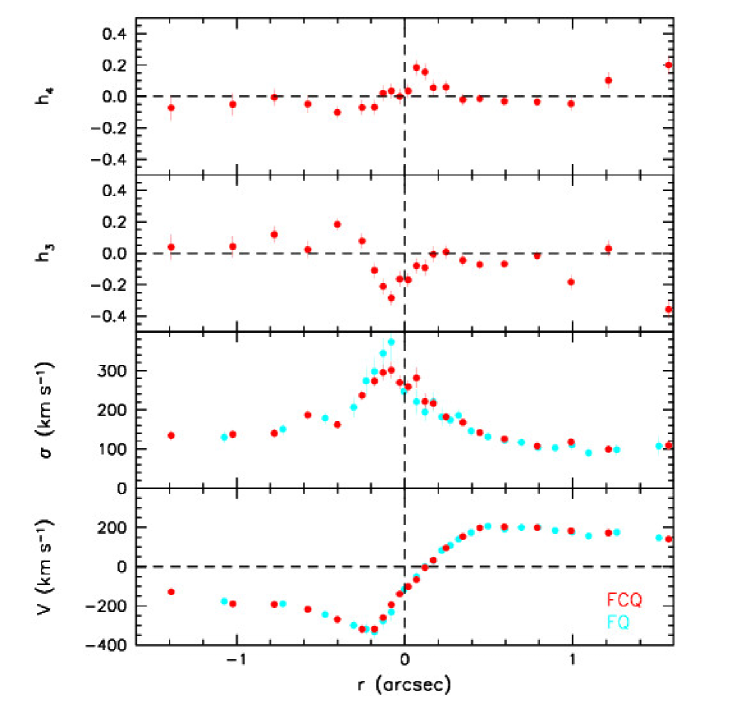
Figure 7.— The red points show the rotation velocity $V$, velocity dispersion $\sigma$, and Gauss-Hermite parameters $h_{3}$ and $h_{4}$ as a function of radius as derived with FCQ from the red spectrum of the nucleus of M 31. The blue points are the FQ results from Figure 2.

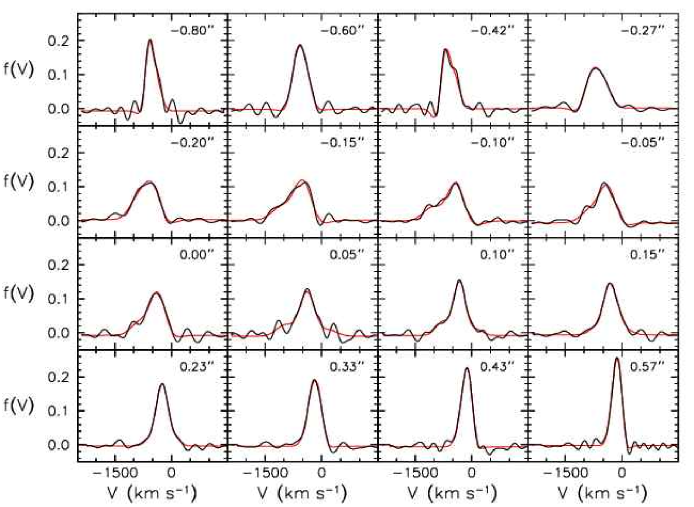
Figure 8.— Line-of-sight velocity distributions in the same radial bins that were used to derive the FCQ kinematic results shown in Figure 19. The black lines are nonparametric LOSVDs; the red curves are the FCQ fits. The radius of the bin is given at upper-right in each panel. At upper-left, we tabulate the velocity dispersion and the Gauss-Hermite parameters $h_{3}$ and $h_{4}$.

Figure 19 compares the FQ and FCQ reductions of the Ca infrared triplet spectra. The velocities are almost identical. The dispersions agree where the higher-order Gauss-Hermite coefficients are small and differ in the expected way when they are not. Where FCQ measures an extended wing of the LOSVD in the prograde direction ($h_{3}<0$ at $r\simeq-0\farcs 1$), it finds a smaller dispersion than FQ, because FQ fits a Gaussian to the whole LOSVD, including wings. Similarly, where $h_{4}>0$ at $r\simeq+0\farcs 1$, FCQ fits a broader Gaussian than FQ and then clobbers the intermediate-velocity shoulders of the Gaussian with $h_{4}$ to make the fitted LOSVD triangular.

Kinematic asymmetries inherent in an eccentric disk provided the basic test of that model in Tremaine (1995), in KB, and in Peiris & Tremaine (2003). We now know that the BH is in the blue nucleus P3 at $r=0$ in Figure 19. Stars in the eccentric disk linger at apocenter to form P1; as a result, both the rotation amplitude $|V|$ and the velocity dispersion $\sigma$ are relatively small at $r\simeq+0\farcs 5$. Other stars in the eccentric disk are passing pericenter slightly on the anti-P1 side of the BH; as a result, the rotation amplitude is large at $r\simeq-0\farcs 2$ in P2. The apparent velocity dispersion is highest at approximately the same radii because the slit and PSF average over stars moving in a variety of directions as they swing around the BH. Figures 11 and 12 in Peiris & Tremaine (2003) show that their nonaligned model accurately accounts for the asymmetric rotation and dispersion profiles.

An important additional property of the LOSVDs – and the unusual one mentioned above – is the observation that $h_{3}$ has the same sign as $V$ over a radius range of $\Delta r\simeq 0\farcs$4 centered $\sim 0\farcs$1 on the anti-P1 side of P3. This effect was seen at ground-based spatial resolution in KB. It is much larger here. It is opposite to the normal behavior of rotating stellar systems, in which velocity projection along the line of sight makes $h_{3}$ antisymmetric with $V$ (van der Marel et al. 1994; Bender, Saglia, & Gerhard 1994). Also, the maximum amplitude, $h_{3}\simeq-0.3$, is unusually large compared to values in other galaxies. All this is easily seen in the LOSVDs (Figure 20; radii $-$0$\farcs$15 and $-$0$\farcs$10) as the broad wings on the $-V$ side of the line centers. These wings tell us that, on the anti-P1 side of the P3, where the average galactic rotation is toward us ($V$ is negative in Figure 20), many stars are rotating more rapidly and few stars are rotating more slowly than the mean rotation velocity averaged within the PSF.

Our interpretation is the same as in KB. The velocity dispersion is expected to look big near pericenter in the eccentric disk, because the slit and PSF integrate over stars that are at different positions along orbits that are rapidly turning around the BH. A prograde LOSVD wing follows naturally if there are many stars still closer to the BH and if they also are in eccentric orbits with apocenters that point toward P1. In the almost-Keplerian potential of the BH, these stars have larger pericenter velocities than the mean $V$ farther out; in fact, their velocities should be larger than the local circular velocity. Consistent with this interpretation, the LOSVD asymmetry is most obvious at $r=-0\farcs 05$ to $-0\farcs 15$, i. e., at slightly more than one PSF radius on the anti-P1 side of P3. The highest velocities reach $\sim 1000$ km s^-1, indeed somewhat larger than what we measure at about the same location for the PSF-blurred velocities of the blue stars in P3. Of course, this explanation only works if the BH is embedded in P3.

The fact that we can understand naturally an observation not predicted by Tremaine (1995) increases our confidence in his model. With improved disk parameters, Peiris & Tremaine (2003, see Figure 13 and 14) accurately predict the $h_{3}$ and $h_{4}$ profiles near the BH. At this point, there seems little doubt that the interpretation of the double nucleus as an eccentric disk is correct and that its main parameters have been determined. The important next step is self-consistent dynamical models to investigate whether the present configuration can be long-lived (e. g., Statler et al. 1999; Statler 1999; Bacon et al. 2001, Salow & Statler 2004). A larger black hole mass. as estimated here, will likely help to construct more long lived models. Beyond that, the origin of the eccentric disk remains essentially unknown.

Table 4

Kinematics of M 31 derived from the red CaT spectra with the Fourier Quotient method

radius	V	$\Delta$V	$\sigma$	$\Delta\sigma$
arcsec	km s-1	km s-1	km s-1	km s-1
$-1.075$	$-177$	14	130	15
$-0.726$	$-189$	13	151	14
$-0.474$	$-244$	13	179	14
$-0.304$	$-299$	23	207	24
$-0.230$	$-319$	32	274	35
$-0.180$	$-332$	34	298	38
$-0.130$	$-276$	36	345	39
$-0.080$	$-232$	45	373	48
$-0.005$	$-118$	23	247	25
$0.070$	$-52$	28	221	31
$0.120$	$0$	22	195	23
$0.170$	$32$	23	220	26
$0.220$	$84$	21	182	23
$0.270$	$108$	14	174	15
$0.320$	$140$	15	186	17
$0.396$	$175$	10	146	11
$0.495$	$207$	8	131	8
$0.595$	$192$	7	122	8
$0.694$	$200$	7	117	8
$0.794$	$200$	7	104	8
$0.894$	$185$	9	103	11
$0.994$	$178$	11	111	13
$1.094$	$156$	10	91	12
$1.262$	$175$	11	99	13
$1.513$	$147$	19	108	23

Table 5

Kinematics of M 31 derived from the red CaT spectra with the Fourier Correlation Quotient method

radius	V	$\Delta$V	$\sigma$	$\Delta\sigma$	$h_{3}$	$\Delta h_{3}$	$h_{4}$	$\Delta h_{4}$
arcsec	km s-1	km s-1	km s-1	km s-1
$-1.390$	$-130.8$	11.7	135.4	10.6	$0.040$	0.079	$-0.092$	0.079
$-1.023$	$-189.6$	11.0	140.0	11.6	$0.056$	0.072	$-0.043$	0.072
$-0.776$	$-192.2$	8.3	144.2	10.2	$0.110$	0.053	$0.013$	0.053
$-0.578$	$-217.0$	11.2	188.7	11.8	$0.037$	0.054	$-0.046$	0.054
$-0.401$	$-267.2$	7.2	168.3	7.1	$0.168$	0.039	$-0.070$	0.039
$-0.254$	$-316.4$	12.7	240.2	12.2	$0.082$	0.048	$-0.074$	0.048
$-0.180$	$-313.6$	14.4	279.6	15.5	$-0.089$	0.047	$-0.035$	0.047
$-0.130$	$-247.9$	16.3	296.5	22.1	$-0.188$	0.050	$0.060$	0.050
$-0.080$	$-181.4$	16.1	300.7	23.1	$-0.264$	0.049	$0.084$	0.049
$-0.030$	$-137.6$	14.5	273.7	18.2	$-0.147$	0.048	$0.026$	0.048
$0.020$	$-99.0$	13.0	263.9	17.3	$-0.156$	0.045	$0.051$	0.045
$0.070$	$-59.6$	15.6	286.1	27.5	$-0.061$	0.050	$0.194$	0.050
$0.120$	$-4.8$	12.6	226.0	21.5	$-0.072$	0.051	$0.176$	0.051
$0.170$	$36.0$	13.0	231.1	18.4	$-0.001$	0.051	$0.079$	0.051
$0.246$	$96.2$	8.4	184.9	11.5	$0.009$	0.041	$0.062$	0.041
$0.346$	$152.2$	7.0	170.3	8.2	$-0.042$	0.038	$-0.007$	0.038
$0.446$	$198.2$	4.8	143.3	5.7	$-0.075$	0.031	$-0.002$	0.031
$0.592$	$203.6$	3.5	126.1	3.9	$-0.072$	0.025	$-0.021$	0.025
$0.788$	$199.2$	3.5	109.2	3.8	$-0.016$	0.029	$-0.029$	0.029
$0.989$	$185.5$	5.7	117.0	6.1	$-0.185$	0.045	$-0.037$	0.045
$1.213$	$173.6$	5.9	103.1	8.2	$0.014$	0.052	$0.075$	0.052
$1.569$	$140.3$	7.0	108.7	12.5	$-0.379$	0.059	$0.221$	0.059

References

- (1)
- (2) Aparicio, A., Gallart, C. 2004, AJ, 128, 1465
- (3)
- (4) Bacon, R., Emsellem, E., Monnet, G., & Nieto, J.-L. 1994, A&A, 281, 691
- (5)
- (6) Bacon, R., et al. 2001, A&A, 371, 409
- (7)
- (8) Bender, R. 1990, A&A, 229, 441
- (9)
- (10) Bender, R., Saglia, R. P., & Gerhard, O. E. 1994, MNRAS, 269, 785
- (11)
- (12) Bertola, F., Bressan, A., Burstein, D., Buson, L. M., Chiosi, C., & di Serego Alighieri, S. 1995, ApJ, 438, 680
- (13)
- (14) Binney, J., Tremaine, S. 1987, Galactic Dynamics, Princeton University Press, Princeton, New Jersey
- (15)
- (16) Bower, G. A., et al. 2001, ApJ 550, 75
- (17)
- (18) Brown, G. E., & Bethe, H. A. 1994, ApJ, 423, 659
- (19)
- (20) Brown, T. M., Ferguson, H. C., Stanford, S. A., & Deharveng, J.-M. 1998, AJ, 504, 113
- (21)
- (22) Bruzual, G., Charlot, S. 2003, MNRAS, 344, 1000
- (23)
- (24) Corbin, M. R., O’Neil, E., & Rieke, M. J. 2001, AJ, 121, 2549
- (25)
- (26) Cox, A. N., ed. 1999, Allen’s Astrophysical Quantitites (New York: Springer)
- (27)
- (28) Crane, P. C., Dickel, J. R., Cowan, J. J. 1992, ApJ, 390, L9
- (29)
- (30) Crane, P. C., Cowan, J. J., Dickel, J. R., & Roberts, D. A. 1993a, ApJ, 417, L61
- (31)
- (32) Crane, P., et al. 1993b, AJ, 106, 1371
- (33)
- (34) Davidge, T. J., Rigaut, F., Doyon, R., & Crampton, D. 1997, AJ, 113, 2094
- (35)
- (36) Dressler, A. 1984, ApJ, 286, 97
- (37)
- (38) Dressler, A., & Richstone, D. O. 1988, ApJ, 324, 701
- (39)
- (40) Emsellem, E., Combes, F. 1997, A&A, 323, 674
- (41)
- (42) Ferrarese, L., & Merritt, D. 2000, ApJ, 539, L9
- (43)
- (44) Finley, D. S., Koester, D., & Basri, G. 1997, ApJ, 488, 375
- (45)
- (46) Gebhardt, K., et al. 2000a, AJ, 119, 1157
- (47)
- (48) Gebhardt, K., et al. 2000b, ApJ, 539, L13
- (49)
- (50) Gebhardt, K., et al. 2003, ApJ, 583, 92
- (51)
- (52) Genzel, R., et al. 1998, ApJ, 498, 579
- (53)
- (54) Genzel, R., et al. 2003, ApJ, 594, 812
- (55)
- (56) Ghez, A. M., et al. 2003, ApJ, 586, L127
- (57)
- (58) Ghez, A. M., et al. 2004, ApJ, in press (astro-ph/0306130)
- (59)
- (60) Goudfrooij, P., Baum, S. A., & Walsh, J. R. 1997, in The 1997 HST Calibration Workshop, ed. S. Casertano et al. (Baltimore: STScI), 100
- (61)
- (62) Iben, I., Tutukov, A. V., & Yungelson, L. R. 1996, ApJ, 456, 750
- (63)
- (64) Jacobs, V., & Sellwood, J. A. 2001, ApJ, 555, L25
- (65)
- (66) King, I. R., et al. 1992, ApJ, 397, L35
- (67)
- (68) King, I. R., Stanford, S. A., & Crane, P. 1995, AJ, 109, 164
- (69)
- (70) Kleinman, S.J., et al. 2004, ApJ 607, 426
- (71)
- (72) Koester, D., et al. 2001, A&A 378, 556
- (73)
- (74) Kormendy, J. 1987, in IAU Symposium 127, Structure and Dynamics of Elliptical Galaxies, ed. T. de Zeeuw (Dordrecht: Reidel), 17
- (75)
- (76) Kormendy, J. 1988, ApJ, 325, 128
- (77)
- (78) Kormendy, J. 2004, in Carnegie Observatories Astrophysics Series, Vol. 1, Coevolution of Black Holes and Galaxies, ed. L. C. Ho (Cambridge: Cambridge Univ. Press), in press
- (79)
- (80) Kormendy, J., & Bender, R. 1999, ApJ, 522, 772 (KB)
- (81)
- (82) Kormendy, J., Bender, R., & Bower, G. 2002, in The Dynamics, Structure and History of Galaxies, ed. G. S. Da Costa & H. Jerjen (San Francisco: ASP), 29
- (83)
- (84) Kormendy, J., & Gebhardt, K. 2001, in 20th Texas Symposium on Relativistic Astrophysics, ed. J. C. Wheeler & H. Martel (Melville: AIP), 363 (KG)
- (85)
- (86) Kormendy, J., & Kennicutt, R. C. 2004, ARA&A, 42, 603
- (87)
- (88) Kormendy, J., et al. 2005, in preparation
- (89)
- (90) Lauer, T. R., et al. 1993, AJ, 106, 1436
- (91)
- (92) Lauer, T. R., et al. 1996, AJ, 110, 2622
- (93)
- (94) Lauer, T. R., et al. 2004, astro-ph/0412040
- (95)
- (96) Lauer, T. R., et al. 1998, AJ, 116, 2263
- (97)
- (98) Le Borgne, J.-F., Bruzual, G., Pello, R., Lancon, A., Rocca-Volmerange, B, Sanahuja, B., Schaerer, D., Soubiran, C., & Vilchez-Gomez, R. 2003, A&A, 402, 433
- (99)
- (100) Light, E. S., Danielson, R. E., & Schwarzschild, M. 1974, ApJ, 194, 257
- (101)
- (102) Magorrian, J., et al. 1998, AJ, 115, 2285
- (103)
- (104) Maoz, E. 1995, ApJ, 447, L91
- (105)
- (106) Maoz, E. 1998, ApJ, 494, L181
- (107)
- (108) Morris, M. 1993, ApJ, 408, 496
- (109)
- (110) Mould, J., Graham, J., Matthews, K., Soifer, B. T., & Phinney, E. S. 1989, ApJ, 339, L21
- (111)
- (112) Nieto, J.-L., Macchetto, F. D., Perryman, M. A. C., di Serego Alighieri, S., & Lelièvre. G. 1986, A&A, 165, 189
- (113)
- (114) Peiris, H. V., & Tremaine, S. 2003, ApJ, 599, 237
- (115)
- (116) Pickles, A. J. 1998, PASP, 110, 863
- (117)
- (118) Rich, R. M., Mighell, K. J., Neill, J. D., & Freedman, W. L. 1996, in New Extragalactic Perspectives in the New South Africa, ed. D. L. Block & J. M. Greenberg (Dordrecht: Kluwer), 325
- (119)
- (120) Richstone, D., Bower, G., & Dressler, A. 1990, ApJ, 353, 118
- (121)
- (122) Salow, R. M., Statler, T. S. 2001, ApJ, 551, L49
- (123)
- (124) Salow, R. M., Statler, T. S. 2004, ApJ, 611, 245
- (125)
- (126) Salpeter, E. E. 1955, ApJ, 121, 161
- (127)
- (128) Sambhus, N., & Sridhar, S. 2002, A&A, 388, 766
- (129)
- (130) Sanders, R. H. 1998, MNRAS, 294, 35
- (131)
- (132) Schmidt M. 1959, ApJ, 129, 243
- (133)
- (134) Schödel, R., et al. 2002, Nature, 419, 694
- (135)
- (136) Schödel, R., Ott, T., Genzel, R., Eckart, A., Mouawad, N., & Alexander, T. 2003, ApJ, 596, 1015
- (137)
- (138) Schwarzschild, M. 1979, ApJ, 232, 236
- (139)
- (140) Sérsic, J. L. 1968, Atlas de Galaxias Australes (Cordoba: Observatorio Astronomico, Universidad de Cordoba)
- (141)
- (142) Statler, T. S. 1999, ApJ, 524, L87
- (143)
- (144) Statler, T. S., King, I. R., Crane, P., & Jedrzejewski, R. I. 1999, AJ, 117, 894
- (145)
- (146) Stevenson, D. J. 1991, ARA&A, 29, 163
- (147)
- (148) Thomas, J., Saglia, R. P., Bender, R., Thomas, D., Gebhardt, K., Magorrian, J., Richstone, D. 2004, MNRAS, 353, 391
- (149)
- (150) Tonry, J. L. 1984, ApJL, 283, L27
- (151)
- (152) Tonry, J. L. 1987, ApJ, 322, 632
- (153)
- (154) Tonry, J. L., et al. 2001, ApJ, 546, 681
- (155)
- (156) Toomre, A. 1964, ApJ, 139, 1217
- (157)
- (158) Tremaine, S. 1995, AJ, 110, 628
- (159)
- (160) Tremaine, S. 2001, AJ, 121, 1776
- (161)
- (162) Tremaine, S., et al. 2002, ApJ, 574, 740
- (163)
- (164) van der Marel, R. P., et al. 1997, Nature, 385, 610
- (165)
- (166) van der Marel, R. P., Cretton, N., de Zeeuw, T., & Rix, H.-W. 1998, ApJ, 493, 613
- (167)
- (168) van der Marel, R. P., Rix, H.-W., Carter, D., Franx, M., White, S. D. M., & de Zeeuw, T, 1994, MNRAS, 268, 521
- (169)
- (170) Verolme, E. K., Cappellari, M., Copin, Y., van der Marel, R. P., Bacon, R., Bureau, M., Davies, R. L., Miller, B. M., & de Zeeuw, P. T. 2002, MNRAS, 335, 517
- (171)
- (172) Yu, Q. 2003, MNRAS, 339, 189
- (173)
- (174) Zapolsky, H. S., & Salpeter, E. E. 1969, ApJ, 158, 809
- (175)