A class of self-gravitating, magnetized accretion disks

Abstract

The steady-state structure of self-gravitating, magnetized accretion disks is studied using a set of self-similar solutions which are appropriate in the outer regions. The disk is assumed to be isothermal and the magnetic field outside of the disk is treated in a phenomenological way. However, the internal field is determined self-consistently. The behaviour of the solutions are investigated by changing the input parameters of the model, i.e. mass accretion rate, coefficients of viscosity and resistivity, and the magnetic field configuration.

1 Introduction

One of the key physical ingredients in accretion disks is self-gravity. It plays a significant role in many such systems, ranging from protostellar disks to Active Galactic Nuclei (AGN). The radial and vertical equations for the disk structure are significantly modified because of the possible impact of the self-gravity, although traditional models of accretion disks ignore self-gravity just for simplicity (e.g., Pringle 1981). Nevertheless, Deviations from Keplerian rotation in some AGN and the flat infrared spectrum of some T Tau stars can both be described by self-gravitating disk models.

Because of the complexity of the equations and in order to obtain analytical results, authors have studied the effects related to disk self-gravity either in the vertical structure of the disk (e.g., Bardou et al. 1998) or in the radial direction (e.g., Bodo & Curir 1992). In a situation where we lack strong empirical evidence for the detailed mechanisms involved, Bertin (1997) proposed a new class of self-gravitating disks for which efficient cooling mechanisms are assumed to operate so that the disk is self-regulated at a condition of approximate marginal Jeans stability. Thus, the energy equation is replaced by a self-regulation prescription. He showed that in the absence of a central point mass, there is a set of self-similar solutions describing the steady-state structure of such self-regulated accretion disks. The self-similar solution corresponds to a flat rotation curve, while the disk has a fixed opening angle. In fact, Bertin’s self-similar solution is a generalization of the self-similar solution for self-gravitating disks (Mestel 1963) dominated by viscosity.

Subsequent analysis confirmed the validity of this simple self-similar solution (Bertin & Lodato 1999). Moreover, such kinds of self-regulated accretion disk can successfully describe the spectral energy distribution of protostellar disks (Lodato & Bertin 2001). Recently, Lodato & Rice (2004) studied the transport associated with gravitational instabilities in a relatively cold disk using numerical simulations. They showed that the disk truly settles into a self-regulated state, where the axisymmetric stability parameter $Q\approx 1$ and where transport and energy dissipation are dominated by self-gravity. However, these studies neglected the possible effects of magnetic fields. Many authors tried to construct models for magnetized disk either in a phenomenological way based on some physical considerations (e.g., Schwartzman 1971; Lovelace et al. 1994; Kaburaki 2000; Shadmehri 2004; Shadmehri & Khajenabi 2005) or by direct numerical simulations (Stone et al. 1999; McKinney & Gammie 2002). Bisnovatyi-Kogan & Lovelace (2000) suggested that recent papers discussing Advection-Dominated Accretion Flow (ADAF) as a possible solution for astrophysical accretion should be treated with caution, particularly because of our ignorance surrounding the magnetic field. Models of magnetized accretion disks with externally imposed large scale vertical magnetic field and anomalous magnetic field due to enhanced turbulent diffusion have also been studied (see, e.g., Campbell 2000; Ogilvie & Livio 2001). These models are restricted to subsonic turbulence in the disk and the viscosity and magnetic diffusivity are due to hydrodynamic turbulence.

Recently, we presented a set of analytical self-similar solutions for the steady-state structure of a magnetized, radiation-dominated disk (Shadmehri & Khajenabi 2005). Although this analysis is just a simple model, one can see some possible effects of the magnetic field on the structure of radiation-dominated disks, at least at a fundamental level. However, we applied some simplifying assumptions concerning the magnetic field both outside and inside of the disk. Our approach was based on interesting studies by Lovelace et al. (1987) and Lovelace et al. (1994). We noticed that it is possible to take a similar approach to study magnetized, self-gravitating disk.

In this paper, we relax the self-regulation condition of Bertin (1997) simply by assuming an isothermal equation of state. We present self-similar solution for the steady-state structure of such self-gravitating disk for which the effect of the magnetic field is taken into account. While the magnetic field outside of the disk is studied in a phenomenological approach similar to Lovelace et al. (1994), the magnetic field inside the disk is obtained self-consistently. We show that magnetic fields may cause significant changes in the typical behaviours of the solutions compared to the nonmagnetized case. The basic equations of the model are described in section 2. Self-similar solutions are obtained in section 3. In spite of the similarity of Bertin’s solutions (1997) to ours, there are differences between his work and the present analysis. A summary of results are discussed in the final section.

2 General Formulation

The basic equations are integrated over the vertical thickness of the disk. The mass continuity equation becomes

$$-2\pi R\Sigma v_{\rm R}=\dot{M},$$ (1)

where $v_{\rm R}$ is the radial velocity and $\Sigma=\int dz\rho\simeq 2h\rho$ is the surface density of the disk. The half-thickness is denoted by $h$, where we consider the magnetic field effect on the disk thickness. We will see that the disk can be compressed or flattened depending on the field configuration. Also, we note that since the radial velocity is negative for accretion (i.e., $v_{\rm R}<0$), the accretion rate $\dot{M}$ as an input parameter of our model is positive.

The radial momentum equation reads

$$\Sigma v_{\rm R}\frac{dv_{\rm R}}{dR}-\Sigma\frac{v_{\varphi}^{2}}{R}=-\frac{dP}{dR}-\Sigma\frac{GM(R)}{R^{2}}+\int F_{\rm R}^{\rm mag}dz,$$ (2)

where $P=\int dzp$ is the integrated disk pressure and $M(R)$ is the mass of the disk within radius $R$ . We are neglecting the mass of the central object comparing to the disk mass. This is relevant to protostellar disks at the beginning of the accretion phase during which the mass of the central object is small and self-gravity of the disk plays an important role. Also, one may argue that our model corresponds to disks at large radii because the effects of the central mass become unimportant in the outer regions of the disk. The term associated with self-gravity of the disk, i.e. $GM(R)/R^{2}$, is generally applicable to spherical geometry. In fact, the correct term takes on an integral form (see equation (4) of Bertin 1997). But, as we will show, our solution describes a disk in which the surface density is inversely proportional to radius. Interestingly, for such a disk which resembles a Mestel disk, the correct gravitational force is known which is exactly equal to our approximate formula (Binney & Tremaine 1987). It implies that we consider the exact gravity force in our equations. Now, we can write

$$\frac{dM(R)}{dR}=2\pi R\Sigma.$$ (3)

The last term of equation (2) represents the height-integrated radial magnetic force which can be written as (Lovelace et al. 1994; hereafter LRN)

$$\int F_{\rm R}^{\rm mag}dz=\frac{1}{2\pi}(B_{\rm R}B_{\rm z})_{\rm h}-\frac{1}{4\pi R^{2}}\frac{d}{dR}[hR^{2}<B_{\varphi}^{2}-B_{\rm R}^{2}>]$$

$$-\frac{1}{4\pi}\frac{d}{dR}[h<B_{\rm z}^{2}>]+\frac{1}{4\pi}\frac{dh}{dR}(B_{\varphi}^{2}+B_{\rm z}^{2}-B_{\rm R}^{2})_{\rm h},$$ (4)

where $<\cdots>\equiv\int_{-h}^{h}dz(\cdots)/(2h)$, and the $h$ subscript denotes that the quantity is evaluated at the upper disk plane, i.e. $z=h$. Similarly, integration over $z$ of the azimuthal equation of motion gives

$$R\Sigma v_{\rm R}\frac{d}{dR}(Rv_{\varphi})=\frac{d}{dR}[R^{3}\nu\Sigma\frac{d}{dR}(\frac{v_{\varphi}}{R})]+\int R^{2}F_{\varphi}^{\rm mag}dz,$$ (5)

where

$$\int R^{2}F_{\varphi}^{\rm mag}dz=\frac{1}{2\pi}(R^{2}B_{\varphi}B_{\rm z})_{\rm h}-\frac{1}{2\pi}\frac{dh}{dR}(R^{2}B_{\rm R}B_{\varphi})_{\rm h}$$

$$+\frac{1}{2\pi}\frac{d}{dR}[hR^{2}<B_{\rm R}B_{\varphi}>].$$ (6)

Here, the last term of equation (5) represents the height-integrated toroidal component of magnetic force multiplied by $R^{2}$.

In our model, we also assume (Shakura & Sunyaev 1973)

$$\nu=\alpha c_{\rm s}h,$$ (7)

where $c_{\rm s}$ is the local sound speed and $\alpha$ is a constant less than unity.

The $z$ component of equation of motion gives the condition for vertical hydrostatic balance, which can be written as

$$\frac{\Sigma}{h}c_{\rm s}^{2}=\pi G\Sigma^{2}+(\frac{1}{4\pi})[(B_{\rm R})_{\rm h}^{2}+(B_{\varphi})_{\rm h}^{2}]-\frac{h}{4\pi}(B_{\rm R})_{\rm h}\frac{dB_{\rm z}}{dR},$$ (8)

where the term on the left hand side of the above equation corresponds to the thermal pressure. Since we neglect the central object, the self-gravity of the disk in the vertical direction leads to the first term on the right hand side of the above equation. Now, we can treat the internal magnetic field using the induction equation. LRN showed that the variation of $B_{\rm z}$ with $z$ within the disk is negligible for even field symmetry. Moreover, $B_{\rm R}$ and $B_{\varphi}$ are odd functions of $z$ and consequently $\partial B_{\rm R}/\partial z\approx(B_{\rm R})_{\rm h}/h$ and $\partial B_{\varphi}/\partial z\approx(B_{\varphi})_{\rm h}/h$. Krasnopolsky & Konigl (2002) applied similar configurations to study the time-dependent collapse of magnetized, self-gravitating disks. Thus,

$$B_{\rm R}(R,z)=\frac{z}{h}(B_{\rm R})_{\rm h},B_{\varphi}(R,z)=\frac{z}{h}(B_{\varphi})_{\rm h},$$

$$B_{\rm z}(R,z)=B_{\rm z}(R),$$ (9)

and the induction equation reads

$$-RB_{\rm z}v_{\rm R}-\frac{\eta R}{h}(B_{\rm R})_{\rm h}+\eta R\frac{dB_{\rm z}}{dR}=0,$$ (10)

where the magnetic diffusivity $\eta$ has the same units as kinematic viscosity. We assume that the magnitude of $\eta$ is comparable to that of the turbulent viscosity $\nu$ (e.g., Bisnovatyi-Kogan & Ruzmaikin 1976; Shadmehri 2004). Exactly in analogy to the alpha prescription for $\nu$, we are using a similar form for the magnetic diffusivity $\eta$,

$$\eta=\eta_{0}c_{\rm s}h,$$ (11)

where $\eta_{0}$ is a constant. Note that $\eta$ is not constant and depends on the physical variables of the flow, and in our self-similar solutions, as we will show, $\eta$ scales with radius as a power law. This form of scaling for diffusivity has been widely used by many authors (e.g., Lovelace, Wang & Sulkanen 1987; Lovelace, Romanova & Newman 1994; Ogilvie & Livio 2001; Rüdiger & Shalybkov 2002).

While equation (10) describes the transport of a large-scale magnetic field (here, $B_{\rm z}(R)$), the values of $(B_{\rm R})_{\rm h}$ and $(B_{\varphi})_{\rm h}$ are determined by the field solutions external to the disk. Instead, we are following the approach of LNR, in which the external field solutions obey the relations

$$(B_{\rm R})_{\rm h}=\beta_{\rm r}B_{\rm z},(B_{\varphi})_{\rm h}=\beta_{\varphi}B_{\rm z},$$ (12)

where $\beta_{\rm r}$ and $\beta_{\varphi}$ are constants of order unity ($\beta_{\varphi}<0$). Thus, one can simply show that $<B_{\rm R}^{2}>=\beta_{\rm r}^{2}B_{\rm z}^{2}/3$, $<B_{\varphi}^{2}>=\beta_{\varphi}^{2}B_{\rm z}^{2}/3$ and $<B_{\rm R}B_{\varphi}>=\beta_{\rm r}\beta_{\varphi}B_{\rm z}^{2}/3$. Note that these beta factors are really empirical scalings which now have abundant support from computer simulations of MHD and Poynting outflows from disks. Ustyugova et al. (1999) gives a detailed analysis and provides strong evidence for $\beta_{\rm r}\sim|\beta_{\varphi}|\sim 1$.

To close the equations of our model, we can write the self-regulation condition as has been done by Bertin (1997). But one should naturally expect another form of self-regulation prescription in the magnetized case. In fact, self-regulation results from a competition of dissipation and instabilities. Indeed, the instability of a magnetized disk is different from that of unmagnetized disk. Effects of the magnetic field on linear gravitational instabilities in two-dimensional differentially rotating disks have been investigated in detail by Elmegreen (1987, 1994), Gammie (1996) and Fan & Lou (1997). Axisymmetric and nonaxisymmetric perturbations show significantly different behaviours. While axisymmetric instability in a thin disk borrows its physical grounds from Toomre (1964) and requires $Q<1$, the literature has lacked an explicit theoretical evaluation of critical $Q$ for nonaxisymmetric gravitational runaways. In order to avoid such difficulties one can consider the axisymmetric stability. The presence of the magnetic fields modifies the Toomre criterion for a hydrodynamic disk in such a way that magnetized disks are unstable to axisymmetric perturbation if $Q_{\rm M}=Q(1+1/\beta)<1$, where $\beta$ is the ratio of the thermal pressure to the magnetic pressure (e.g., Shu 1992).

There is a fundamental point concerning the self-regulation prescription. When the disk mass becomes large enough to induce global instability there is nothing like self-regulation taking place. We can see numerical simulations which describe massive unstable disk (e.g., Bonnell 1994; Matsumoto & Hanawa 2003). However, considering existing numerical simulations, we think, it is not possible simply to say that all massive disks fragment because, to our knowledge, not only current numerical simulations suffer from their own limitations, but also they do not generally give a fully consistent picture as for global fragmentation. This situation becomes more complicated when we consider magnetic fields. It seems that there is a complicated interaction between gravitational instability and MHD turbulence that influences disk structure, but MHD turbulence reduces the strength of the gravitational instability (Fromang 2005).

Almost all numerical simulations show that global instabilities are highly depend on the thermal state of the disk (Gammie 2001, Johnson & Gammie 2003). However, thermal state of the disk has been neglected by some authors and so their approach is not a complete analysis. Simulations by Mastsumoto & Hanawa (2003) which do not include detailed thermal evolution, predict fragmentation in an early phase. But all these fragments are on tight orbits and are likely to merge due to disk accretion. Matzner & Levin (2005) argue analytically that viscous heating and stellar irradiation quenches fragmentation and conclude that numerical simulations lead to fragmentation which do not account for irradiation and are unrealistic. On the other hand, not necessarily all numerical simulations of massive disks lead to fragmentation. For example, Pickett at al. (2000) failed to obtain fragmentation in similar thermodynamics condition. Thus, whether or not massive disks fragment due to global instability remains controversial. At this stage what we can say is that even if a massive disk with no star in the center does not fragment, it does not mean that self-regulation is occurring in the disk. In order to avoid such difficulties, we relax the self-regulation condition and replace it by an isothermal assumption, i.e.

$$P=\Sigma c_{\rm s}^{2},$$ (13)

where $c_{\rm s}$ is constant sound speed. We hope our simple approach will be able to illustrate some possible effects of the magnetic fields on the structure of self-gravitating disks.

3 Self-similar solutions

Equations (1), (2), (3), (5), (8), (10) and (13) constitute the basic equations of our model for the steady-state structure of self-regulated magnetized disk. We can solve these equations numerically using appropriate boundary conditions. However, before doing such an analysis it would be illustrative to study the typical behaviour of the solutions by applying semi-analytical methods, e.g. self-similarity. Indeed, any self-similar solution contains part of the behavior of the system, in particular far from the boundaries. However the main goal of our analysis is just to illustrate the possible effects of the magnetic field on the steady-state structure of a self-gravitating disk. For this propose, we think, self-similar solutions are very useful.

It is then straightforward to find a self-similar solution with the radial dependence

$$\frac{\Sigma(R)}{\Sigma_{0}}=a(\frac{R}{R_{0}})^{-1},$$ (14)

$$\frac{v_{\varphi}(R)}{V_{0}}=b,$$ (15)

$$\frac{v_{\rm R}(R)}{V_{0}}=-c,$$ (16)

$$\frac{P(R)}{P_{0}}=d(\frac{R}{R_{0}})^{-1},$$ (17)

$$\frac{B_{\rm z}(R)}{B_{0}}=e(\frac{R}{R_{0}})^{-1},$$ (18)

$$\frac{h(R)}{R_{0}}=f(\frac{R}{R_{0}}),$$ (19)

$$\frac{M(R)}{M_{0}}=q(\frac{R}{R_{0}}),$$ (20)

with $a$, $b$, $c$, $d$, $e$, $f$ and $q$ being numerical constants which can be obtained from the equations (see below). Also, $R_{0}$, $\Sigma_{0}$, $P_{0}$, $V_{0}$ and $B_{0}$ are convenient units which reduce the equations into non-dimensional forms. We are assuming $V_{0}=c_{\rm s}=\sqrt{P_{0}/\Sigma_{0}}$ and $M_{0}=R_{0}^{2}\Sigma_{0}$.

If we substitute the above self-similar solutions in the main equations of the model, the following system of dimensionless algebraic equations are obtained which are to be solved for $a$, $b$, $c$, $d$, $e$, and $f$:

$$ac=\dot{m},$$ (21)

$$-(ab^{2}+d)=-2a^{2}+[2\beta_{\rm r}+\frac{2}{3}f(3+\beta_{\varphi}^{2}-\beta_{\rm r}^{2})]e^{2},$$ (22)

$$ab(\alpha f\sqrt{\frac{d}{a}}-c)=\beta_{\varphi}(2-\frac{4}{3}f\beta_{\rm r})e^{2},$$ (23)

$$\frac{d}{f}=a^{2}+(f\beta_{\rm r}+\beta_{\rm r}^{2}+\beta_{\varphi}^{2})e^{2},$$ (24)

$$c-\eta_{0}\beta_{\rm r}\sqrt{\frac{d}{a}}-\eta_{0}\sqrt{\frac{d}{a}}f=0,$$ (25)

$$d=a,$$ (26)

where $\dot{m}$, $\alpha$, $\eta_{0}$, $\beta_{\rm r}$ and $\beta_{\varphi}$ are the input parameters. Also, $\dot{m}=\dot{M}/(2\pi R_{0}\Sigma_{0}V_{0})$ is the nondimensional mass accretion rate. The radial dependence of physical quantities both in the magnetized and the unmagnetized cases are similar. After some algebraic manipulations we can find a complicated algebraic equation for $f$ and clearly only the real root is a physical solution. Having the real root of this equation, the other physical quantities are determined using the above equations.

Now, we explore the parameter space of the input parameters and their effects on the solutions. We restrict our study to values around unity for $\beta_{\rm r}$ and $\beta_{\varphi}$ (Ustyugova et al. 1999). Since we find that the sensitivity of solutions on the parameter $\beta_{\varphi}$ is not very strong, we plot all the physical variables as a function of $\beta_{\rm r}$ for a fixed $\beta_{\varphi}$. However, we comment about possible effects of variations of $\beta_{\varphi}$ by the final figure.

Figure 1 shows various physical variables as function of $\beta_{\rm r}$ with $\alpha=0.1$, $\eta_{0}=0.1$, $\beta_{\varphi}=-0.8$ and the mass accretion rate is indicated on the plots. This figure helps us to see the dependence of the physical variables on the variations of the mass accretion rate $\dot{m}$. The plots on the top show surface density (left) and the opening angle (right) for $\dot{m}=0.5$, $1.0$ and $2.0$. We see as the parameter of the radial component of the magnetic field at the surface of the disk increases, the surface density decreases for a fixed mass accretion rate. But the surface density increases by increasing $\dot{m}$. Also, as the mass accretion rate increases, the disk becomes thinner. However, the disk thickness increases with $\beta_{\rm r}$ for a fixed accretion rate. The plots on the middle show typical behaviors of the radial and the rotational velocities. While the ratio of the radial velocity to the sound speed increases with increasing $\beta_{\rm r}$, the ratio of the rotational velocity to the sound speed decreases keeping $\dot{m}$ constant. However, increasing the mass accretion rate causes the radial velocity to decrease. But for the rotational velocity, we see completely different behaviour, i.e. the ratio $v_{\varphi}/c_{\rm s}$ significantly increases with the accretion rate $\dot{m}$.

Our self-similar solution generally corresponds to $\beta>1$, where $\beta$ is the ratio of thermal pressure to magnetic pressure at the surface of the disk. The plot on the bottom of Figure 1 (left) shows this behavior, although $\beta$ decreases with $\beta_{\rm r}$ for a fixed $\dot{m}$. However, if the accretion rate increases the ratio of the thermal pressure to the magnetic pressure $\beta$ increases which implies the effect of the magnetic field on the structure becomes weaker. We have already discussed about the Toomre parameter $Q$ and a modified version of this parameter, i.e. $Q_{\rm M}$ because of the magnetic field. Figure 1 shows variation of both $Q$ and $Q_{\rm M}$ as function of $\beta_{\rm r}$ (curves corresponding to $Q_{\rm M}$ are shown by dotted lines). Generally, we have $Q_{\rm M}>Q$ because of the dynamical effects of the magnetic field and as $\beta_{\rm r}$ increases these parameters increases to values closer to unity or even higher values. It implies a more stable disk according to the Toomre criteria as $\beta_{\rm r}$ increases. Also, the Toomre parameter rapidly increases when the mass accretion rate decreases.

The $\eta_{0}$-dependence of the solutions is shown in the Figure 2. In fact, this Figure is similar to Figure 1 except for changing the input parameter $\eta_{0}$ to different values $0.05$, $0.1$ and $0.2$. The other input parameter are the same as in Figure 1. The surface density $\Sigma$, the rotational velocity $v_{\varphi}$ and the ratio $\beta$ decrease with increasing $\eta_{0}$. But the radial velocity $v_{\rm R}$ increases with increasing $\eta_{0}$. We see that as $\eta_{0}$ tends to the larger values, the disk thickness increases. Also, for a fixed $\eta_{0}$ the disk thickness increases as $\beta_{\rm r}$ increases, however, the ratio $h/R$ is more sensitive to the variation of $\beta_{\rm r}$ for higher values of $\eta_{0}$. Interestingly, as the magnetic diffusivity coefficient $\eta_{0}$ increases, the Toomre parameters $Q$ and $Q_{\rm M}$ significantly increase to values higher than unity.

The $\alpha$-dependence of the solutions is not strong as long as $\beta_{\rm r}\approx|\beta_{\varphi}|\approx 1$. But we found that the ratio $\beta$ and the Toomre parameter change because of viscosity variations. Figure 3 (top, left) shows $\beta$ as a function of $\beta_{\rm r}$. Clearly, as the viscosity parameter $\alpha$ increases, the ratio $\beta$ increases. Also, the Toomre parameter increases with the viscosity parameter. We found that $\beta_{\varphi}$-dependence of the solutions is weak for $|\beta_{\varphi}|\approx 1$. However, there is some changes on the ratio $\beta$ as $\beta_{\varphi}$ varies. Figure 3 (bottom, left) shows variation of $\beta$ as a function of $\beta_{\rm r}$ for $\beta_{\varphi}=-0.8$, $-1.0$ and $-1.2$. Evidently, this ratio increases with $|\beta_{\varphi}|$. Also, by increasing $|\beta_{\varphi}|$ the Toomre parameter increases, though it is not very significant.

Bertin (1997) showed that the opening angle of self-regulated nonmagnetized disk depends only on $Q$, independent of the viscosity coefficient and the mass accretion rate. He argued that significantly large values of $Q$ would be undesirable because they conflict with the thin disk approximation. But the disk thickness in our magnetized case depends on the mass accretion rate and the other input parameters as long as the beta factors are of order unity. For larger values of $\beta_{\rm r}$ or $\beta_{\varphi}$, the disk thickness may change because of the magnetic fields.

4 Conclusions

We have obtained a self-similar solution for a self-gravitating, magnetized, viscous disk. The solution has constant rotational and accretion velocities, independent of the radial distance. Since we are considering an isothermal magnetized disk, the sound speed is constant.

Our goal is to study the possible effects of the magnetic fields on the steady state structure of self-gravitating, magnetized disk, at least at the physical level. Although we have made some simplifying assumptions in order to treat the problem analytically, our self-similar solution shows magnetic fields can really change typical behaviour of the physical quantities of a self-gravitating disk. Not only the surface density of the disk changes, but also the rotational and the radial velocities significantly change because of the magnetic fields. It means any realistic model for self-gravitating disk should consider the possible effects of the magnetic fields. Of course, our self-similar solutions are too simple to make any comparison with observations. But, we think, one may relax self-similarity assumption and solve the equations of the model numerically. In doing so, our self-similar solutions can greatly facilitate testing and interpretation of results. Then, we can calculate the spectral energy distribution of such a self-gravitating magnetized disk.

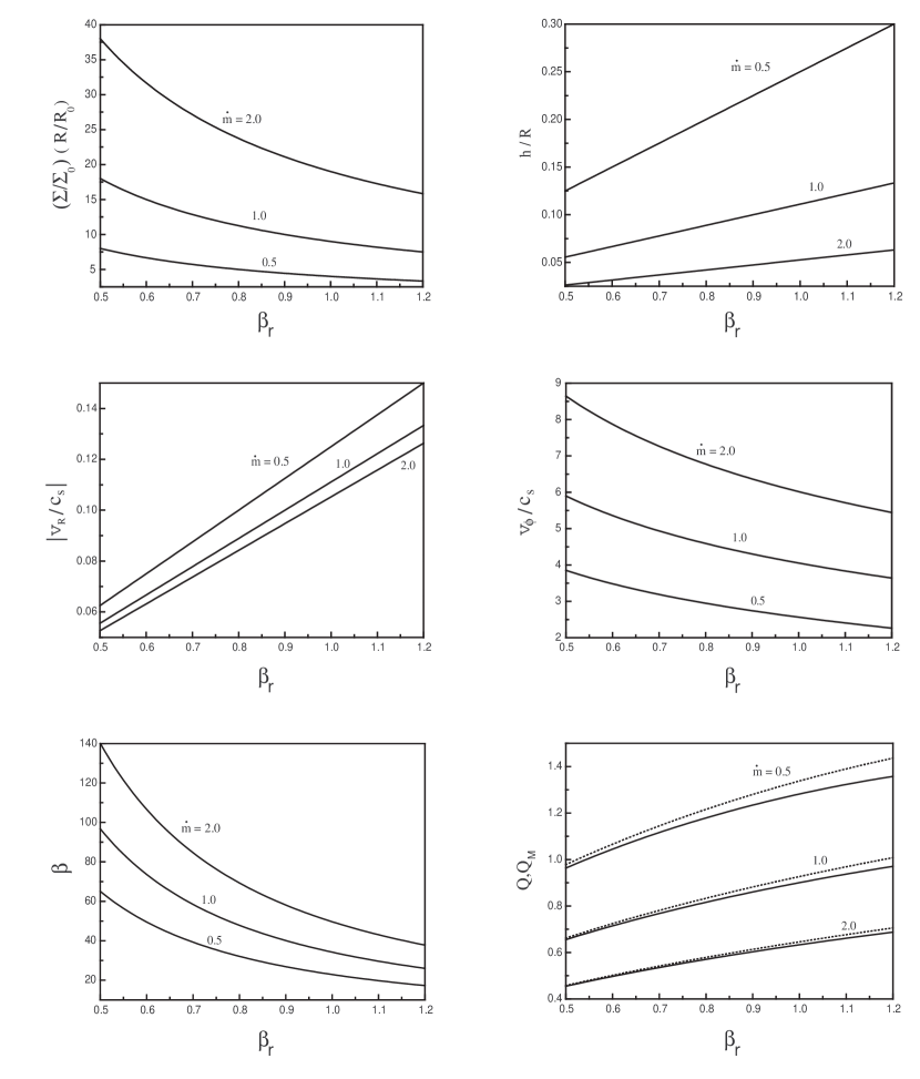
Figure 1: Typical behaviours of the surface density (top, left), opening angle of the disk (top, right), ratios of the radial and the rotational velocities to the sound speed (middle), ratio of the thermal pressure to the magnetic pressure at the surface (bottom, left) and the Toomre parameters corresponding to $\alpha=0.1$, $\eta_{0}=0.1$, $\beta_{\varphi}=-0.8$ and the other input parameters are indicated on the plots. Magnetic Toomre parameter $Q_{\rm M}$ is denoted by the dotted lines. These plots show the effects of the mass accretion rate $\dot{m}$ on the structure of the disk.

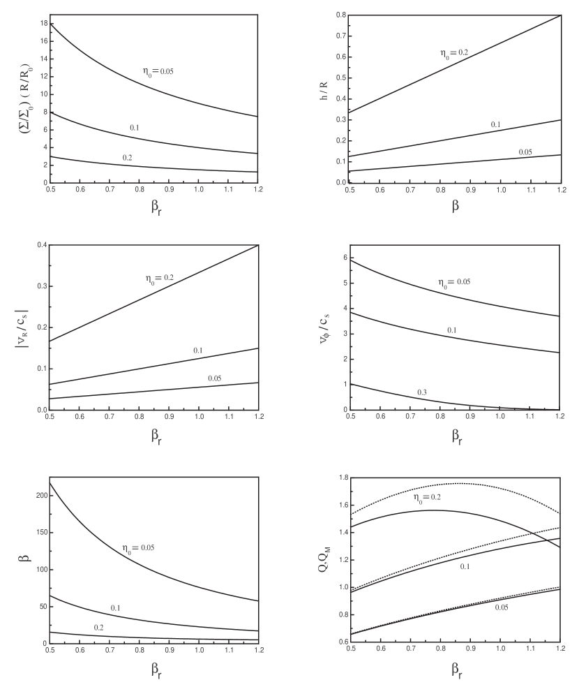
Figure 2: The same as Figure 1, but for $\dot{m}=0.5$, $\alpha=0.1$, and $\beta_{\varphi}=-0.8$. These plots show the effects of magnetic diffusivity coefficient $\eta_{0}$ on the solutions. Also, the magnetic Toomre parameter is denoted by dotted lines.

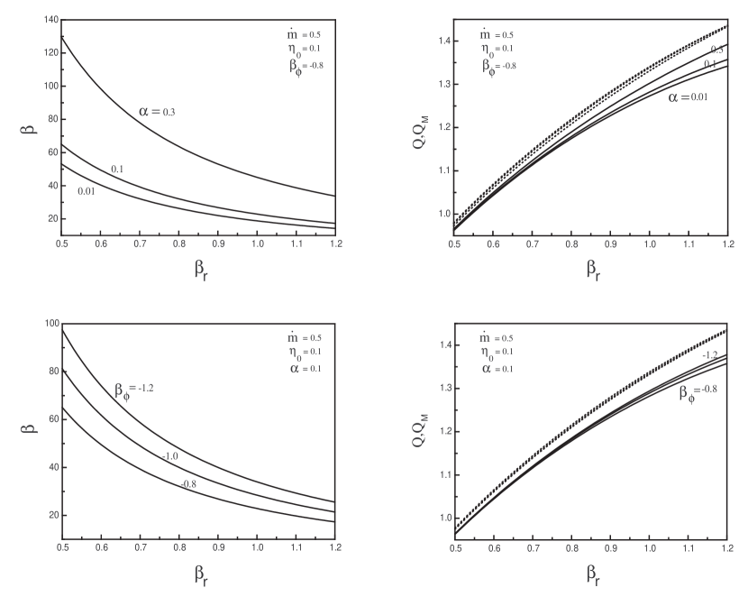
Figure 3: Top plots show the effects of the viscosity parameter $\alpha$ on the structure of the disk. Among the physical variables describing the disk, however, the ratio of the thermal pressure to the magnetic pressure at the surface of the disk $\beta$ and the Toomre parameters are more sensitive to the variations of the viscosity coefficient. We have similar behaviour when the parameter $\beta_{\varphi}$ varies, i.e. the ratio $\beta$ and the Toomre parameters $Q$ and $Q_{\rm M}$ are more sensitive to the variations of $\beta_{\varphi}$ keeping the rest of the input parameters fixed (bottom plots).

References

- (1)
- (2) Binney, J., Tremaine, S. 1987, Galactic Dynamics, Princeton University Press, Princeton
- (3)
- (4) Bardou, A., Heyvaerts, J., Duschl, W. J. 1998, A&A, 337, 966
- (5)
- (6) Bertin, G. 1997, ApJ, 478, L71
- (7)
- (8) Bertin, G., Lodato, G. 1997, A&A, 350, 694
- (9)
- (10) Bisnovatyi-Kogan, G. S., Lovelace, R. V. E. 2000, ApJ, 529, 978
- (11)
- (12) Bodo, G., Curir, A. 1992, A&A, 253, 318
- (13)
- (14) Bonnell, I. A. 1994, MNRAS, 269, 837
- (15)
- (16) Campbell, C. G. 2000, MNRAS, 317, 501
- (17)
- (18) Krasnopolsky, R., Konigl, A. 2002, ApJ, 580, 987
- (19)
- (20) Elmegreen, B. G. 1987, ApJ, 312, 626
- (21)
- (22) Elmegreen, B. G. 1994, ApJ, 433, 39
- (23)
- (24) Fan, Z. H., Lou, Y.-Q. 1997, MNRAS, 291, 91
- (25)
- (26) Fromang, S. 2005, A&A, in press (astro-ph/0506216)
- (27)
- (28) Gammie, C. F. 1996, ApJ, 462, 725
- (29)
- (30) Gammie, C. F. 2001, ApJ, 553, 174
- (31)
- (32) Johnson, B. M., Gammie, C. F. 2003, ApJ, 597, 131
- (33)
- (34) Kaburaki, O. 2000, ApJ, 531, 210
- (35)
- (36) Matsumoto, T., Hanawa, T. 2003, ApJ, 595, 913
- (37)
- (38) Matzner, C. D., Levin, Y. 2005, ApJ, 628, 817
- (39)
- (40) McKinney, J. C., Gammie, C. F. 2002, ApJ, 573, 728
- (41)
- (42) Mestel, L. 1963, MNRAS, 126, 553
- (43)
- (44) Lodato, G., Bertin, G. 2001, A&A, 375, 455
- (45)
- (46) Lodato, G., Rice, W. K. M.,, 2004, MNRAS, 351, 630
- (47)
- (48) Lovelace, R. V. E., Romanova, M. M., Newman, W. I. 1994, ApJ, 437, 136 (LRN)
- (49)
- (50) Lovelace, R. V. E., Wang, J. C. L., Sulkanen, M. E. 1987, ApJ, 315, 504
- (51)
- (52) Ogilvie, G. I., Livio, M. 2001, ApJ, 553, 158
- (53)
- (54) Pickett, B., Durisen, R., Cassen, P., Mejia, A. 2000, ApJ, 540, L95
- (55)
- (56) Pringle, J. 1981, ARA&A, 19, 137
- (57)
- (58) Rüdiger, G., Shalybkov, D. A. 2002, A&A, 393, L81
- (59)
- (60) Shadmehri, M. 2004, A&A, 424, 379
- (61)
- (62) Shadmehri, M. Khajenabi, F. 2005, MNRAS, 361, 719
- (63)
- (64) Shakura, N. I., Sunyaev, R.A. 1973, A&A, 24, 337
- (65)
- (66) Shu, F. H. 1992, The Physics of Astrophysics. II. Gas Dynamics (Mill Valley: Univ. Science Books)
- (67)
- (68) Shvartsman, V. F. 1971, Soviet Astron., 15, 377
- (69)
- (70) Stone, J. M., Pringle, J. E., Begelman, M. C. 1999, MNRAS, 310, 1002
- (71)
- (72) Ustyugova, G. V., Koldoba, A. V., Romanova, M. M., Chechetkin, V. M., Lovelace, R. V. E. 1999, ApJ, 516, 221
- (73)
- (74) Toomre, A. 1964, ApJ, 139, 1217
- (75)