Gravitational Wave Background from Neutrino-Driven Gamma-Ray Bursts

Abstract

We discuss the gravitational wave background (GWB) from a cosmological population of gamma-ray bursts (GRBs). Among various emission mechanisms for the gravitational waves (GWs), we pay a particular attention to the vast anisotropic neutrino emissions from the accretion disk around the black hole formed after the so-called failed supernova explosions. The produced GWs by such mechanism are known as burst with memory, which could dominate over the low-frequency regime below $\sim 10$Hz. To estimate their amplitudes, we derive general analytic formulae for gravitational waveform from the axisymmetric jets. Based on the formulae, we first quantify the the spectrum of GWs from a single GRB. Then, summing up its cosmological population, we find that the resultant value of the density parameter becomes roughly $\Omega_{\mathrm{GW}}\approx 10^{-20}$ over the wide-band of the low-frequency region, $f\sim 10^{-4}-10^{1}$Hz. The amplitude of GWB is sufficiently smaller than the primordial GWBs originated from an inflationary epoch and far below the detection limit.

1 Introduction

The observation of gravitational waves (GWs) is one of the most important missions to explore the trackless parts of the Universe. Several ground-based laser interferometers (TAMA300, LIGO, and GEO600) are now operating and taking continuously the data at a frequency range, 10Hz – 10kHz, where rapidly-moving stellar objects accompanied with strong gravity, such as formations of neutron stars or black holes, are the most promising sources for GWs (See New (2003) for a review). The Laser Interferometer Space Antenna, LISA covering $10^{-4}-10^{-2}$ Hz will be launched near future, and moreover, the future space missions such as BBO or DECIGO (Seto et al., 2001) target the frequency window around 0.1Hz. For such interferometers, the primordial GWs generated during an inflationary epoch could be detected. Also, these interferometers are expected to be useful in determining the cosmic equation of the state (Takahashi & Nakamura, 2005). Thus, low-frequency GWs detected via space interferometers may provide a powerful cosmological tool to probe the extremely early Universe (Maggiore, 2000). One important remark is that several astrophysical foregrounds around deci-Hertz band proposed so far are believed to be weak or resolvable (e.g., Ferrari et al., 1999; Schneider et al., 2001; Farmer & Phinney, 2003).

Recently, however, Buonanno et al. (2004) pointed out the possibility that a cosmological population of core-collapse supernovae could contaminate the inflationary GWs at the low-frequency range mentioned above, as a result of the GW associated with the neutrino emissions. Their analysis suggests that even in a deci-hertz band, one may not simply neglect the contributions from the cosmological stellar objects, especially with the asymmetric emissions of neutrinos. The important remark is that GWs from neutrino-driven jets are generated by different emission mechanisms from those of the periodic GWs. For an energy flow originating from a burst, the GW amplitude suddenly rises from zero and settles down into a non-vanishing value after the burst. This phenomenon is called burst with memory (Braginsky & Thorne, 1987). It has been argued that a burst of neutrinos released anisotropically can generate a burst of GW accompanying with the memory effect. A cosmological contribution of such GW may therefore become significant at the low-frequency band rather than the high-frequency regime.

Among several candidates other than the core-collapse supernovae, GRBs are expected to have powerful asymmetric jets with the enormous emission of high energy neutrinos. It has been already pointed out that relativistic jets of matter associated with GRBs can generate strong GWs enough to be detected by the present laser interferometers (Sago et al., 2004). In fact, a data analysis searching for GWs associated with the very bright GRB030329 have been performed by LIGO group (Abbott et al., 2005), although they reported a null result.

Another important aspect is that these jets are thought to be driven by thermal energy deposition due to the neutrino and anti-neutrino annihilation into electrons and positrons, which occurs primarily at the polar region of the black hole-accretion disk system, namely, the neutrino-driven GRBs (Paczynski, 1990; Meszaros & Rees, 1992; Popham et al., 1999; Ruffert & Janka, 1999; MacFadyen & Woosley, 1999; Asano & Fukuyama, 2000) (see, Proga et al., 2003; Mizuno et al., 2004; Takiwaki et al., 2004, for the MHD processes). Naively inferred from the energetics of core-collapse supernovae (Burrows & Hayes, 1996; Fryer et al., 2004; Müller et al., 2004; Kotake et al., 2005), anisotropic energy flows from the GRBs also become important sources of GWs, in addition to the anisotropic jets of the matter itself (Sago et al., 2004). While a cosmological contribution of those GWs may not play a significant role due to the relatively rare event rate of the GRBs, a quantitative estimate of the shape and the amplitude of the spectrum still remains important issue to clarify the nature of gravitational wave background arising from the memory effect. We then wish to understand how the GW memory is generated and how much amount of the GWs is released from a cosmological population of GRBs in an analytic manner.

The purpose of this paper is to give an analytic estimate of the gravitational wave spectrum from the GW memory effect, particularly focusing on the neutrino-driven GRBs. In Sec.2, after briefly describing the axisymmetric jet model, we derive a general analytic formula for gravitational waveform with memory effect from the asymmetric relativistic jets, which is both applicable to the ultra-relativistic and the relativistic cases. Using this formula, in Sec.3, we compute the spectrum of GWs from a single neutrino-driven GRB. Then, in Sec.4, summing up a cosmological population of GRBs, we estimate the amplitude of gravitational wave background (GWB). Uncertainties of the model parameters are also taken into account when evaluating the GWB, and we find that the resultant GWB amplitude becomes rather small and would be difficult to detect by the present and future missions of GW observatories. Finally, summary and discussion are devoted to section 5.

2 Gravitational Waves from relativistic Jets

In this paper, we specifically treat the GWs from the ultra-relativistic jets, particularly focusing on the neutrino-driven GRBs as a plausible GW source. In this case, energy sources powering the GRBs rely on the neutrino emission from the accreting disk (Piran, 2002, for a review and references therein). Recently, Setiawan et al. (2004) performed the three-dimensional hydrodynamic simulations and obtained the time evolution of the luminosity of neutrinos emitted from accretion disks around hyper-accreting stellar-mass black hole. Using their results, Aloy et al. (2004) performed the two-dimensional simulations to study the evolution of relativistic jets driven by thermal energy deposition due to $\nu\overline{\nu}$-annihilation. In next section, we adopt their fitting result for the neutrino luminosity evolution to calculate the GW amplitude. Before estimating this, we discuss the GW memory and derive a general analytic formula for gravitational waveform from the axisymmetric relativistic jets.

According to the memory effect of GWs, the GW amplitude $h(t)$ jumps from zero to a non-vanishing value and it keeps maintaining the non-vanishing value even after the energy source of GWs disappears. Epstein (1978) has derived a general formula of memory effect produced by the radial emission of neutrinos. The detectability of such effect was discussed by Braginsky & Thorne (1987) through the ground-based laser interferometers. Recently, Segalis & Ori (2001) studied the memory effect generated by a point particle whose velocity changes via gravitational interactions with other objects. Further, Sago et al. (2004) estimated the amplitude of GW memory from the GRB jets based on the internal shock model. Here, we consider the GWs from the neutrino-driven GRB and derive a useful analytic formula for the axisymmetric emission of neutrinos.

Let us introduce the two coordinate systems shown in figure 1; the source coordinate system $(x^{\prime},y^{\prime},z^{\prime})$ and the observer coordinate system $(x,y,z)$. In these coordinate systems, the $z^{\prime}$-axis is chosen as jet axis, while the $z$-axis is set to a line-of-sight direction. Further, the origins of these two coordinate systems are set to the centre of a GRB object. Then, the viewing-angle denoted by $\xi$ is given by the angle between $z$- and $z^{\prime}$-axis. For convenience, we assume that the $z$-axis lies on the $(x^{\prime},z^{\prime})$-plane. In this case, the two polarization states of GWs satisfying the transverse-traceless conditions become $h_{+}\equiv h_{xx}=-h_{yy}$ and $h_{\times}\equiv h_{xy}=h_{yx}$ in the observer coordinates and we obtain $h_{\times}=0$ (see below). Note that the sum of the squared amplitudes, $|h_{+}|^{2}+|h_{\times}|^{2}$, is invariant under the rotation about the $z$-axis. The geometrical setup shown in figure 1 yields the following relation between the two polar coordinate systems $(\theta,\phi)$ and $(\theta^{\prime},\phi^{\prime})$:

$$\sin\theta^{\prime}\cos\phi^{\prime}=\sin\theta\cos\phi\cos\xi+\cos\theta\sin\xi,$$

$$\sin\theta^{\prime}\sin\phi^{\prime}=\sin\theta\sin\phi,$$

$$\cos\theta^{\prime}=-\sin\theta\cos\phi\sin\xi+\cos\theta\cos\xi.$$ (1)

Since the GRBs are cosmological, one can safely neglect the time lag between the two points near the source region, i.e., $|t-t^{\prime}|\ll r/c$ (Müller & Janka, 2004). Thus the amplitude of GWs observed by the distant observer may be written as

$$h_{+}(t)=\frac{2G}{c^{4}r}\int^{t-r/c}_{-\infty}\!dt^{\prime}d\Omega^{\prime}\,\psi(\Omega^{\prime})\frac{dL}{d\Omega^{\prime}}(\Omega^{\prime},t^{\prime}),\quad$$ (2)

$$\psi(\Omega^{\prime})=\frac{\beta^{2}\sin^{2}\theta}{1-\beta\cos\theta}\cos 2\phi,$$ (3)

where $\beta$ is the velocity of matter in a jet normalized by $c$, and $\theta$ and $\phi$ are related to $\theta^{\prime}$ and $\phi^{\prime}$ through the relation (1). The function $\psi(\Omega^{\prime})$ represents the dependence of the amplitude on the direction of the energy flow (Segalis & Ori, 2001). Note that the counter part of the amplitude, $h_{\times}$, is obtained just replacing $\cos 2\phi$ with $\sin 2\phi$ in equation (3), which immediately yields $h_{\times}=0$ by integrating over the angle $\phi^{\prime}$. The quantity $dL/d\Omega^{\prime}$ is the neutrino luminosity per unit solid angle emitted from the source. For an axisymmetric neutrino emission, we consider the two axisymmetric jets whose luminosity is uniformly distributed with respect to the opening angle of jets. Denoting the opening angle by $\theta_{\rm open}$, we have

$$\frac{dL}{d\Omega}(\Omega,t)=\frac{E}{\Delta\Omega_{\rm jet}}\Gamma(t)$$

$$\qquad\times\left[\Theta\left(\frac{\theta_{\rm open}}{2}-\theta^{\prime}\right)+\Theta\left(\theta^{\prime}-\pi+\frac{\theta_{\rm open}}{2}\right)\right],$$ (4)

where the function $\Theta(\theta)$ is Heaviside step function. The quantity $E$ is the total isotropic emission energy, which is typically $E\simeq\gamma mc^{2}\approx 10^{51}$ erg in the case of jets from relativistic matter, and $E_{\nu}\la 10^{52}$ erg in the case of neutrino emission (Popham et al., 1999). In equation (4), $\Delta\Omega_{\rm jet}$ denotes the solid angle of two jets given by $\Delta\Omega_{\rm jet}\equiv 4\pi\{1-\cos(\theta_{\rm open}/2)\}$. The function $\Gamma(t)$ represents the time dependence of the luminosity of the ejected matter or neutrinos, which will be given explicitly.

Substituting equation (4) into equation (3) and performing the Fourier transformation $2\pi if\widetilde{h}(f)=\int_{-\infty}^{\infty}\!\dot{h}(t)e^{-2\pi ift}\,dt$, the characteristic amplitude defined by $h_{c}(f)\equiv f\widetilde{h}(f)$ is given by

$$h_{c}(f) = \frac{G}{\pi c^{4}r}\frac{\Psi}{\Delta\Omega_{\rm jet}}E|\widetilde{\Gamma}(f)|$$

$$= 8.5\times 10^{-21}\left(\frac{10{\rm kpc}}{r}\right)\left(\frac{E}{10^{52}{\rm erg}}\right)\frac{\Psi}{\Delta\Omega_{\rm jet}}|\widetilde{\Gamma}(f)|.$$

Here, the function $\tilde{\Gamma}(f)$ is the Fourier transform of the function $\Gamma$. The quantity $\Psi$ is the angular integral of the function $\psi(\Omega^{\prime})$, which depends on the parameters, $\theta_{\rm open},\xi$ and $\beta$:

$$\Psi \equiv \int_{\rm jet}\!d\Omega^{\prime}\,\psi(\Omega^{\prime})$$

$$= -\frac{2\pi}{\beta\sin^{2}\xi}\bigg{\{}-2\beta\lambda(1+\cos^{2}\xi)$$

$$\;+\left(\beta\lambda-\cos\xi\right)\sqrt{(\beta\cos\xi-\lambda)^{2}+(1-\beta^{2})(1-\lambda^{2})}$$

$$\;+\left(\beta\lambda+\cos\xi\right)\sqrt{(\beta\cos\xi+\lambda)^{2}+(1-\beta^{2})(1-\lambda^{2})}\bigg{\}}$$

with $\lambda$ being $\cos(\theta_{\rm open}/2)$. In performing the integration, the range of the integral denoted by “jet” is restricted to the jet region, i.e., $0<\theta^{\prime}<\theta_{\rm open}/2$ and $\pi-\theta_{\rm open}/2<\theta^{\prime}<\pi$. In the ultra-relativistic limit ($\beta\to 1$), this yields

$$\Psi=\begin{cases}\displaystyle 4\pi\lambda\left(\frac{1-|\cos\xi|}{\sin\xi}\right)^{2}&{\rm for}~{}{|\cos\xi|}>{\lambda},\\ \displaystyle 4\pi(1-\lambda)\frac{\lambda-\cos^{2}\xi}{\sin^{2}\xi}&{\rm for}~{}|\cos\xi|\leq\lambda.\end{cases}$$ (7)

Figure 2 illustrates the viewing-angle dependence of the GW amplitude $\Psi/\Delta\Omega_{\rm jet}$, in the cases of relativistic ($\beta=0.9$) and ultra-relativistic limit ($\beta=1.0$). Figure 2 clearly shows that the intensity of the GWs generated from an axisymmetric relativistic jet has an anti-beaming distribution. Compared to the relativistic case ($\beta<1)$, the anti-beaming feature of ultra-relativistic jet is very sensitive to the opening angle, while the viewing-angle dependence becomes fairly weak for a typical value of the opening angle, $\theta_{\rm open}\leq\pi/6$ (Frail et al., 2001). This indicates that the GWs from the neutrino-driven GRB are uniformly emitted in contrast to the axisymmetric emission of the neutrinos itself.

Analytic expression (2) with (2) and (7) is one of the main result in this paper. It describes the gravitational waveform generated from a (ultra-)relativistic emission of neutrinos and/or matter with opening angle $\theta_{\rm open}$ and with the velocity $\beta$. With the analytic expression, one can further estimate the GWB spectrum in a tractable manner. Before doing this, we first apply this formula to estimate the amplitude of GW from a single neutrino-driven GRB in next section.

Figure 1: Source coordinate system ($x^{\prime},y^{\prime},z^{\prime}$) and observer coordinate system ($x,y,z$). The observer resides at the distant point on the $z$-axis. The $z^{\prime}$-axis coincides with the symmetric axis of the GRB source. Inside the jet represented by dashed lines, the luminosity of energy flow is assumed to be uniformly distributed with the opening angle $\theta_{\rm open}$.

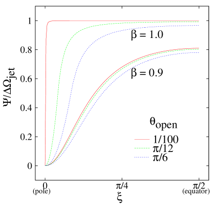
Figure 2: Viewing-angle dependence of the amplitude. The upper three lines represent the ultra-relativistic cases ($\beta=1.0$), and lower ones relativistic cases ($\beta=0.9$). We take three kinds of the opening-angle, $\theta_{\rm open}=1/100,\pi/12,\pi/6$.

3 Gravitational waves from a Single GRB

Provided the time evolution of the luminosity $\Gamma(t)$, the analytic formulae (2) with equation (2) and/or (7) enable us to estimate the frequency dependence of the characteristic amplitude, depending on the parameters $(\xi,\theta_{\rm open},E,r)$. In this section, for a simple but a realistic model of the luminosity evolution, we adopt the fitting result by Aloy et al. (2004) to calculate the GW spectrum from a single GRB.

According to the state-of-the-art three-dimensional hydrodynamic simulations (Setiawan et al., 2004), the fitting function is given by

$$\Gamma(t)=\frac{2}{6t_{\rm f}-t_{\rm b}}\begin{cases}(t/t_{\rm b})&0\leq t<t_{\rm b}\\ 1&t_{\rm b}\leq t<t_{\rm f}\\ (t/t_{\rm f})^{-3/2}&t_{\rm f}\leq t\end{cases},$$ (8)

and $\Gamma(t)=0$ for $t<0$. Here, the time $t_{\rm b}$ roughly corresponds to $t_{\rm b}\approx t_{\rm f}/3$. Note that the three phases of the time evolution in equation (8) are intimately related to the evolutionary phases of the neutrino emission; i) the mass accretion, which makes the luminosity linearly growing, ii) stationary phase after stopping the mass fall, and iii) slow decay by the termination of neutrino production in the accretion disk. These basic behaviors should be fairly insensitive to a detailed modeling of neutrino emission. Although Aloy et al. (2004) only considered a short-duration GRB in which the duration $t_{\mathrm{b}}$ and $t_{\mathrm{f}}$ were set to $0.01$ sec and $0.03$ sec, respectively, we keep to use equation (8) for a long-duration GRB. Additionally, note that the observed duration is a few times larger than the duration $t_{\mathrm{f}}$ due to the tail part of equation (8) at the late time. The observed duration is typically 0.2 sec for short-duration GRBs and 20 sec for long-duration GRBs (Zhang & Mészáros, 2004).

Figure 3 plots typical examples of the characteristic amplitudes for neutrino-driven GRBs. The solid line shows the amplitude of GWs from the GRB located at the Galactic centre ($r=$10kpc), while the short-dashed lines represent the GRBs located at $r=$1Mpc (upper) and 100Mpc (lower). Here, we assume the total isotropic neutrino energy, $E=10^{52}$ erg (Popham et al., 1999), in order to set an upper bound of the contributions from the neutrinos to the GW amplitudes. Further, extrapolating the neutrino luminosity evolution for the short-duration GRBs (Setiawan et al., 2004) to that for the long-duration GRBs, GW amplitude from the long GRB was also calculated by simply setting $t_{\rm f}=10$ sec (solid line, labeled as “Long”).

Clearly from figure 3, the dominant part of the GWs appears at a low-frequency band and they enter the detectable band by future observatories. While the high-frequency part of GWs rapidly falls down, the characteristic amplitude of low-frequency GW asymptotically approaches constant, which implies that Fourier component of GWs $\tilde{h}(f)$ is inversely proportional to the frequency, i.e., $\tilde{h}\propto 1/f$. This behavior typically arises from a sudden change of the neutrino luminosity and can be deduced from the so-called zero-frequency limit of GW memory (e.g., Braginsky & Thorne, 1987; Epstein, 1978; Buonanno et al., 2004).

The results in figure 3 indicate that the planned space interferometers, LISA and practical DECIGO can easily detect the GWs from a GRB at the Galactic centre, though the local GRB rate around the Galaxy is extremely small. The GRB rate would be increased as the observed volume is increasing. For instance, we might observe a few GRB events for a decade within 100Mpc. As shown in the figure, however, the amplitude of GWs from such a far GRB is quite small, which may be comparable or smaller than that of GWs generated in the inflationary epoch. In addition, while one may detect such GW by an ultimate version of the space interferometer whose sensitivity is limited by the quantum noise, the detection of GW memory needs a somewhat different technique from periodic and burst-like GWs, which will be an important subject of GW data analysis.

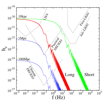
Figure 3: The characteristic amplitude of GWs from a single GRB at the the Galactic centre (solid line). The “Long” duration $t_{\mathrm{f}}$ is 10 sec and “Short” is 0.1 sec (long-dashed line). On the other hand, the short-dashed lines represent the “Long” duration GRB at 1Mpc (upper) and 100Mpc (lower). To compute the GW amplitudes, we specifically set the model parameters to $\xi=\pi/2$, $\theta_{\mathrm{open}}=\pi/6,E=10^{52}$ erg.

4 Estimating the GWB from neutrino-driven GRBs

We are in a position to discuss the contribution of GWs from the neutrino-driven GRBs to the background radiation. We assume that all GRBs have same energy and opening-angle ($\theta_{\rm open}=\pi/6$), and the viewing-angle is randomly distributed. According to Phinney (2001), the sum of the energy densities radiated by a large number of independent GRBs at each redshift is given by the density parameter $\Omega_{\rm GW}(f)\equiv\rho_{c}^{-1}(d\rho_{\rm GW}/d\log f)$ as:

$$\Omega_{\rm GW} = \frac{2\pi^{2}c}{G\rho_{c}}\int_{0}^{\infty}\!dz\,\frac{R_{\rm GRB}(z)}{1+z}\frac{1}{(1+z)H(z)}$$ (9)

$$\times r^{2}f^{3}\langle|\widetilde{h}_{+}(f)|^{2}\rangle_{\xi,t_{\rm f}}\Big{|}_{t_{\rm f}\to t_{\rm f}/(1+z)\atop f\to f(1+z)},$$

with $R_{\rm GRB}(z)$ being redshift distribution of GRBs. $H(z)$ is the Hubble parameter. Here the quantity $\langle|\widetilde{h}_{+}(f)|^{2}\rangle_{\xi,t_{\rm f}}$ represents the averaged value of the amplitude $|\widetilde{h}_{+}(f)|^{2}$ over the viewing-angle $\xi$ and the duration $t_{\rm f}$. Note that the combination $r^{2}f^{2}\langle|\widetilde{h}_{+}(f)|^{2}\rangle_{\xi,t_{\rm f}}$ becomes independent of the distance $r$, and the explicit dependence on the redshift $z$ is eliminated after replacing $(f,t_{\rm f})$ with $(f(1+z),t_{\rm f}/(1+z))$.

In order to quantify the amplitude of GWB, we need the redshift distribution of GRBs. For a crude estimate of the amplitude of $\Omega_{\rm GW}$, we use the redshift evolution inferred from the $E_{p}$-luminosity correlation (Amati et al., 2002; Yonetoku et al., 2004):

$$R_{\rm GRB}(z)\propto\begin{cases}(1+z)^{6.0\pm 1.4}&z<1\\ (1+z)^{0.4\pm 0.2}&z>1\end{cases}.$$ (10)

As for the normalization factor $R_{\rm GRB}(0)$, the local observation by BATSE indicates $10^{-7}$ per year per a galaxy, but, the jets are highly aligned and the true GRB rate must be larger. Then, the local GRB rate becomes $\sim 10^{-5}$ per year per a galaxy (Frail et al., 2001), or equivalently,

$$R_{\rm GRB}(0)=25\sim 250\;{\rm Gpc}^{-3}{\rm yr}^{-1}.$$ (11)

Assuming that the orientation of jets is random, the ensemble average $\langle|\widetilde{h}_{+}(f)|^{2}\rangle_{\xi,t_{\rm f}}$ in equation (9) is evaluated separately, namely, $\langle|\widetilde{h}_{+}(f)|^{2}\rangle_{\xi,t_{\rm f}}\propto\langle|\Psi|^{2}\rangle_{\xi}\langle|\widetilde{\Gamma}(t)|^{2}\rangle_{t_{\rm f}}$. For the average over the viewing-angle $\xi$, one finds

$$\langle|\Psi|^{2}\rangle_{\xi}=\frac{1}{4\pi}\int_{0}^{\pi}\!\Psi(\xi)^{2}\;2\pi\sin\xi\,d\xi.$$ (12)

The integration can be done analytically, but the result is rather complicated. For a typical set of parameters $(\theta_{\rm open},\beta)=(\pi/6,1)$, this gives 0.154. On the other hand, for the average of the GW amplitude over the duration, the distribution function for the duration of GRBs, $T(t_{\rm f})$ must be taken into account. Here, we use the data set of durations ($T_{90}$) taken from the BATSE 4B catalog adopting a logarithmic binning with $\Delta\log_{10}t_{\rm f}=0.1$. The resultant distribution becomes a bimodal distribution over the range 0.015 sec $\leq t_{\rm f}\leq$ 670 sec. Since the function $\widetilde{\Gamma}(f)$ is the only quantity that explicitly depends on the duration $t_{\rm f}$, the ensemble average of the GW amplitude may be independently evaluated as:

$$\langle|\widetilde{\Gamma}(t)|^{2}\rangle_{t_{\rm f}}=\frac{\int\!|\widetilde{\Gamma}(t)|^{2}T(t_{\rm f})\,dt_{\rm f}}{\int\!T(t_{\rm f})\,dt_{\rm f}}.$$ (13)

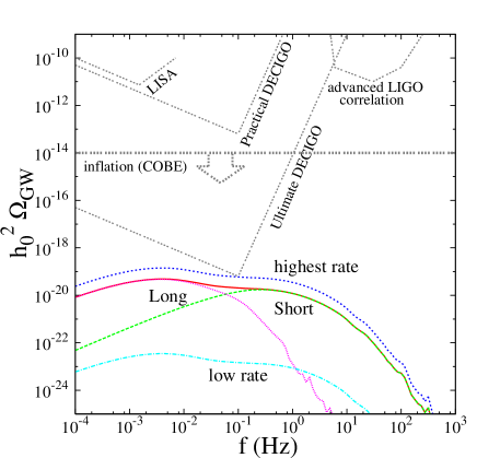
Figure 4: The energy density parameter of GWB. The solid line represents the contribution from neutrinos of all GRBs. The dotted line represents one from “Long”-duration GRBs ($t_{\mathrm{f}}>2$ sec), and the long-dashed line one from “Short”-duration GRBs ($t_{\mathrm{f}}<2$ sec). The dotted-dashed line represents the case of $R_{\mathrm{GRB}}(0)=25\;{\rm Gpc}^{-3}{\rm yr}^{-1}$,$R_{\mathrm{GRB}}\propto(1+z)^{4.6},(1+z)^{0.2}$ (“low rate”). On the other hand, the short-dashed line represents the case of highest GRB rates, $R_{\mathrm{GRB}}(0)=250\;{\rm Gpc}^{-3}{\rm yr}^{-1}$, $R_{\mathrm{GRB}}\propto(1+z)^{7.4},(1+z)^{0.6}$ in the cases of $z<1$ and $z>1$, respectively. The horizontal dotted line shows the GWB from the inflationary epoch constrained by COBE observations.

Figure 4 shows the density parameter of GWB generated from neutrino-driven GRBs (solid line), together with the sensitivity curves for future missions. To plot the result, we adopt the flat cosmological model with the density parameters $\Omega_{M}=0.3$ and $\Omega_{\Lambda}=0.7$. The Hubble parameter is given by

$$H(z)=H_{0}\sqrt{\Omega_{M}(1+z)^{3}+\Omega_{\Lambda}}$$ (14)

with the present Hubble parameter $H_{0}$ being $72$ km s^-1/Mpc. Note that when evaluating the expression (9), the range of the integral is restricted to $0\leq z\leq 20$, since most of the contribution ($\sim 80\%$) to the integral comes from the low redshift GRBs $z\la 4$.

Figure  4 shows that the GWB is broadly distributed over the low-frequency band, $10^{-3}{\rm Hz}<f<10^{1}{\rm Hz}$ with amplitude $h_{0}^{2}\Omega_{\rm GW}\sim 10^{-20}$ and has almost the flat spectrum with small bimodal bump. To see the contribution from short-duration GRBs and long-duration GRBs separately, the ensemble average over the duration (13) is artificially divided into the short duration ($t_{f}\leq 2$ sec) and the long duration ($t_{f}>2$ sec), the results of which are respectively shown in dashed and dotted lines. One then immediately deduces that bimodal shape of the GWB spectrum has originated from a distribution of duration. This is mainly because the low-frequency part of the gravitational waveform shown in figure 3 becomes featureless due to the zero-frequency limit of the memory effect. Although the present result was derived from a specific choice of luminosity evolution (8), the characteristic behavior seen in figure 4 would remain unchanged as long as the collapsar model is applicable to both short- and long-duration GRBs.

Figure 4 indicates that the GWB from neutrino-driven GRBs is much smaller than the upper limit of GWB generated in the inflationary epoch constrained by the COBE observations (the horizontal thick

dotted-line) and also below the detection limit of future space missions. Note that this tiny amplitude can be also deduced from an extrapolation of the discussion by Buonanno et al. (2004) based on the following points; i) the GRB rate is roughly four orders of magnitude smaller than the rate of supernovae and ii) the total released energy by neutrinos used in this paper is thirty times smaller than theirs. According to Buonanno et al. (2004), the maximum amplitude of GWB from cosmological supernovae is estimated as $\Omega_{\rm GW}^{\rm SN}\approx 10^{-12}$ (see Fig. 4 of their paper). Since the density parameter $\Omega_{\rm GW}$ is proportional to $R_{\text{GRB}}(0)E_{\nu}^{2}$ (see Eqs.(2) and (9)), we roughly obtain $\Omega_{\rm GW}^{\rm GRB}\approx 10^{-19}$ in the cosmological GRB case. In this sense, small amplitude of GWB may be a natural outcome from the rare even rate of GRB. On the other hand, nearly flat spectrum of GWB in figure 4 cannot be simply explained by an argument based on the the supernovae case, which may be a unique characteristic of the GRB case.

As examined in figure 4 (thick-dotted and dot-dashed lines), the uncertainty of the normalization in the GRB rate (11) does not change the conclusion. In other words, the GWB generated from a cosmological population of GRBs does not become a preventer of the primordial GWB generated in the inflationary epoch.

5 Summary and Discussion

We have discussed the GWs from axisymmetric relativistic jets of neutrino-driven GRBs. In order to estimate the amplitude of the GWs, we derived the analytic formulae for the gravitational waveform from (ultra-)relativistic energy flow. The analytic expression given in equation (2) with (2) and (7) depends on the viewing-angle $\xi$, the opening-angle of the jet $\theta_{\rm open}$, and the velocity of the flow $\beta$, as well as the time evolution of luminosity $\Gamma(t)$ (or $\tilde{\Gamma}(f)$). Following the fitting result obtained from the state-of-the-art numerical simulations of collapsars, the amplitudes of the GWs from a single GRB are estimated and are found that within the detection limits for the space-based laser interferometers like LISA and DECIGO/BBO, if a GRB occurs at the region within 1Mpc. Since the released energy in the jet region by neutrinos can be greater than that by matter, the low-frequency GWs generated by neutrinos seem to dominate the one by matter studied by Sago et al. (2004). Note that, even if the amplitudes of the GW memory overcome the sensitivity curves of interferometers in the spectra, this does not directly imply the detection of the signals. The detectability should be discussed with a specific data analysis technique for the memory effect. On the other hand, the GWB from a cosmological population of GRBs are obtained by summing up the individual GW of the GRBs, which turns out to be sufficiently smaller than those from the inflationary epoch and a cosmological population of supernovae (Buonanno et al., 2004).

While the sufficiently small amplitude of the GWB would be true, there remain several uncertainties in predicting a precise waveform of the GW from a single GRB jet. In particular, when estimating the GW from a long GRB, we have extrapolated to use the luminosity evolution of neutrinos for a short GRB. Since the efficient mechanism to trigger the long burst is still under debate, one should continue to check the present GRB model in more quantitative way. As a prelude to more realistic luminosity evolutions in the collapsar models, which requires general relativistic multidimensional radiation hydrodynamic simulations, our findings obtained in a semi-analytic manner should be the very first step towards the predictions of the GWs from the collapsars and the following formation of GRBs.

References

- Abbott et al. (2005) Abbott B. et al., 2005, Phys.Rev.D 72, 042002
- Aloy et al. (2004) Aloy M.A., Janka H.-T., Müller, E., 2004, preprint(astro-ph/0408291)
- Amati et al. (2002) Amati L. et al., 2002, A&A, 390, 81
- Asano & Fukuyama (2000) Asano K., & Fukuyama T., 2000, ApJ, 531, 949
- Braginsky & Thorne (1987) Braginsky V.B. & Thorne K.S., 1987, Nature, 327, 123
- Buonanno et al. (2004) Buonanno A., Sigl G., Raffelt G.G., Janka H.-T. & Müller E., 2004, astro-ph/0412000
- Burrows & Hayes (1996) Burrows A., & Hayes J., 1996, Phys.Rev.Lett. 76, 352
- Epstein (1978) Epstein R., 1978, ApJ, 223, 1037
- Farmer & Phinney (2003) Farmer A., J. & Phinney E.S., 2003, MNRAS, 346, 1197
- Fenimore & Ramirez-Ruiz (2001) Fenimore E.E. & Ramirez-Ruiz E., 2000, preprint(astro-ph/0004176)
- Ferrari et al. (1999) Ferrari V., Matarrese S. & Schneider R., 1999, MNRAS, 303, 247
- Frail et al. (2001) Frail D.A. et al., 2001, ApJ, 562, L55
- Fryer et al. (2004) Fryer C.L., Holz D.E., & Hughes S.A., 2004, ApJ, 609, 288
- Kotake et al. (2005) Kotake K., Yamada S. & Sato K., submitted to Phys.Rev.D
- Paczynski (1990) Paczynski B., 1990, ApJ, 363, 218
- Phinney (2001) Phinney E.S., 2001, preprint(astro-ph/0108028)
- Proga et al. (2003) Proga D., MacFadyen A.I., Armitage P.J., & Begelman M.C., 2003, ApJ, 599, L5
- Ruffert & Janka (1999) Ruffert M., & Janka H.-T., 1999, A&A, 344, 573
- MacFadyen & Woosley (1999) MacFadyen A.I., & Woosley S.E., 1999, ApJ, 524, 262
- Maggiore (2000) Maggiore M., 2000, Phys. Rep. 331, 283
- Meszaros & Rees (1992) Meszaros P., & Rees M.J., 1992, MNRAS, 257, 29P
- Mizuno et al. (2004) Mizuno Y., Yamada S., Koide S., & Shibata K., 2004, ApJ, 606, 395
- Müller et al. (2004) Müller E., Rampp M., Buras R., Janka H.-T., & Shoemaker D.H., 2004, ApJ, 603, 221
- Müller & Janka (2004) Müller E. & Janka H.-T., 1997, A&A, 317, 140
- New (2003) New K.C.B., 2003, Living Rev. Relativ. 6, 2
- Piran (2002) Piran T., 2002, preprint(gr-qc/0205045)
- Popham et al. (1999) Popham R., Woosley S.E., & Fryer C., 1999, ApJ, 518, 356
- Sago et al. (2004) Sago N., Ioka K., Nakamura T. & Yamazaki R., 2004, Phys.Rev.D 70, 104012
- Schneider et al. (2001) Schneider R., Ferrari V., Matarrese S. & Portegies Zwart S.F., 2001, MNRAS, 324, 797
- Segalis & Ori (2001) Segalis E.B., & Ori A., 2001, Phys.Rev.D 64, 064018
- Setiawan et al. (2004) Setiawan S., Ruffelt M., Janka H.-Th., 2004, MNRAS, 352, 753
- Seto et al. (2001) Seto N., Kawamura S. & Nakamura T., 2001, Phys.Rev.Lett. 87, 221103
- Takahashi & Nakamura (2005) Takahashi R. & Nakamura T., 2005, Prog.Theor.Phys., 113, 64
- Takiwaki et al. (2004) Takiwaki T., Kotake K., Nagataki S., & Sato K., 2004, ApJ, 616, 1086
- Yonetoku et al. (2004) Yonetoku D., Murakami T., Nakamura T., Yamazaki R., Inoue A.K. & Ioka K., 2004, ApJ, 609, 935
- Zhang & Mészáros (2004) Zhang B. & Mészáros P., 2004, Int. J. Mod. Phys. 19, 2385