Supernova Remnants in the Magellanic Clouds. VI. The DEM L 316 Supernova Remnants

Abstract

The DEM L 316 system contains two shells, both with the characteristic signatures of supernova remnants (SNRs). We analyze Chandra and XMM-Newton data for DEM L 316, investigating its spatial and spectral X-ray features. Our Chandra observations resolve the structure of the northeastern SNR (Shell A) as a bright inner ring and a set of “arcs” surrounded by fainter diffuse emission. The spectrum is well fit by a thermal plasma model with temperature $\sim 1.4$ keV; we do not find significant spectral differences for different regions of this SNR. The southwestern SNR (Shell B) exhibits an irregular X-ray outline, with a brighter interior ring of emission including a bright knot of emission. Overall the emission of the SNR is well described by a thermal plasma of temperature $\sim 0.6$ keV. The Bright Knot, however, is spectrally distinct from the rest of the SNR, requiring the addition of a high-energy spectral component consistent with a power-law spectrum of photon index 1.6–1.8.

We confirm the findings of Nishiuchi et al. (2001) that the spectra of these shells are notably different, with Shell A requiring a high iron abundance for a good spectral fit, implying a Type Ia origin. We further explicitly compare abundance ratios to model predictions for Type Ia and Type II supernovae. The low ratios for Shell A (O/Fe of 1.5 and Ne/Fe of 0.2) and the high ratios for Shell B (O/Fe of 30–130 and Ne/Fe of 8–16) are consistent with Type Ia and Type II origins, respectively. The difference between the SNR progenitor types casts some doubt on the suggestion that these SNRs are interacting with one another.

1 Introduction

The peanut-shaped nebula DEM L 316 was first noted by Mathewson & Clarke (1973) to have a high [S II]/H$\alpha$ ratio, a typical signature of supernova remnants (SNRs). The authors designated the two lobes of this system shells A (the northeastern shell) and B (to the southwest); following this and subsequent work, we shall use the same designations. Mathewson et al. (1983) confirmed that the DEM L 316 system had the optical, radio, and X-ray characteristics typical of SNRs. A multi-wavelength study by Williams et al. (1997) concluded that the most probable scenario for DEM L 316’s unique morphology was that it consisted of a pair of colliding SNRs. Evidence cited in support of this scenario included a change in radio polarization between the two shells, the kinematics of the two shells, multiwavelength morphological features and similar extinctions.

Alternate scenarios for the physical association of the two shells include (a) that the shells are the result of a single explosion into a bi-lobed cavity, or (b) that the shells are isolated SNRs apparently juxtaposed along the line of sight, but in fact spatially separated. Nishiuchi et al. (2001), using a study of combined ROSAT and ASCA X-ray data, noted that the shells were spectrally distinct to an extent which would rule out the single-explosion scenario, and also concluded that, on the basis of its enhanced iron abundance, Shell A was probably the result of a Type Ia SN.

In this paper, we present new Chandra observations of DEM L 316. These observations allow us, for the first time, to spatially resolve the structure of the DEM L 316 remnants, with reasonable spectral resolution over smaller regions. We supplement these data with XMM-Newton observations, which allow us to more reliably determine X-ray spectra for larger regions. §2 describes our observations, while §3 contains our analysis. A discussion of the implications of our findings is given in §4, and those findings are summarized in §5.

2 Observations

We observed DEM L 316 with the Chandra  Advanced CCD Imaging Spectrometer (ACIS) S3 back-illuminated chip (sequence number 500279, observation 2829, 40 ks). Data were reprocessed following procedures recommended by the Chandra X-ray Center (CXC): we removed the afterglow correction, generated a new bad pixel file, and applied corrections for charge-transfer inefficiency (CTI) and time-dependent gain for an instrument temperature of -120 C. We also applied background cleaning using the 5$\times$5 pixel islands of our VFAINT mode observation. The dataset was filtered for high-background times and poor event grades, resulting in a total “good time” interval of 35.6 ks, and restricted to the energy range of 0.3-8.0 keV, where the S3 chip is most sensitive.

Spectral results were extracted from the new event file. Background regions were taken from source-free areas surrounding the SNRs, and the spectra of these background regions were scaled and subtracted from the source spectra. Individual spectra for regions of interest (Table 1), and the corresponding primary and auxiliary response files, were extracted with the ciao acisspec script and analyzed in xspec. Spectra were rebinned by spectral energy to achieve a signal-to-noise ratio of 3 in each bin.

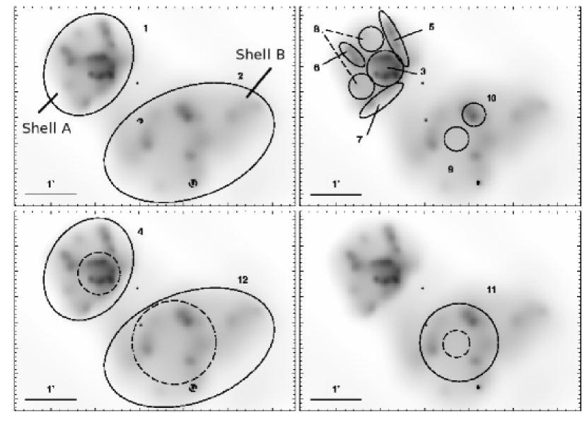
Figure 1: Adaptavely smoothed Chandra ACIS image with spectral regions marked and labeled as listed in Table 1. Regions with dotted lines are excluded from larger regions. Excluded point sources are also shown with dotted lines.

Regions within DEM L 316 were chosen to examine specific morphological features seen in our X-ray images (Figure 1 and Table 1). Regions 1 and 2 enclose the approximate X-ray boundaries of Shell A and Shell B, respectively. Region 3 covers the bright central emission within Shell A, while Region 4 includes the limb of Shell A, excluding that central emission. Regions 5-7 cover brighter X-ray “arcs” to the north, east, and south of Shell A; Region 8 samples emission between those arcs. In Shell B, Region 9 encloses the central emission from the remnant, and Region 10 covers a particularly bright knot of interior emission. Region 11 incorporates the ring-like structure of brighter emission in Shell B, including the bright knot of Region 10. Region 12 covers emission on the limb of Shell B, excluding the center and the ring.

To augment our spectral data for Shells A and B (Regions 1 and 2) we used XMM-Newton EPIC MOS and pn data from observation ID 0201030101, with exposure times of 11.2 ks (MOS1 and MOS2 detectors) and 7.0 ks (pn detector). The pipeline-processed data obtained from the Science Operations Centre (SOC) were reduced using the Science Analysis Software package provided by the SOC. The data were filtered for poor event grades. Spectra for spatial regions corresponding to Regions 1 and 2 in the Chandra observations, and surrounding background regions, were extracted from the filtered event files and rebinned to a minimum of 25 counts per bin. Joint fits were performed in xspec to the data from Chandra’s ACIS and the XMM-Newton instruments.

For comparison, we utilized optical emission-line (H$\alpha$, [S II], [O III]) images taken with the Curtis-Schmidt telescope at Cerro Tololo Inter-American Observatory (CTIO), and radio images from the Australia Telescope Compact Array (ATCA) at 4.4 and 6.0 GHz (7 and 5 cm). The angular resolution of the CTIO images was about 1$\farcs$5; the half-power beamwidth of the radio images was 12″. Other details of these observations are given in Williams et al. (1997).

3 Results

3.1 X-ray Morphologies

Previous X-ray analyses have noted a separation between the X-ray emission from the shells of DEM L 316. In the Chandra ACIS data, we indeed see two distinct shells; any overlap is too close to background levels to constitute a significant detection. Although diffuse emission between the shells is seen in the XMM-Newton observations, this emission is faint ($\sim 2\sigma$ above the background with the EPIC pn); in addition, the SNRs are over 7′ off-axis, and so the spatial resolution may be insufficient to distinguish betwen the boundaries of the two SNRs.

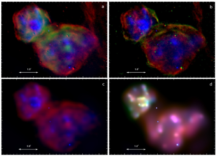
Figure 2: (a) 3-band image showing H$\alpha$ from the CTIO Curtis-Schmidt telescope (red), 7 cm radio map from the ATCA (green), and adaptively smoothed Chandra ACIS image (blue). (b) 3-band image showing H$\alpha$ (red), [O III] (green), and smoothed ACIS image (blue). (c) 2-band image showing ATCA 7 cm (red) and smoothed ACIS image (blue). (d) 3-color Chandra ACIS image showing emission at 0.3-0.8 keV (red), 0.8-1.5 keV (green), and 1.5-8.0 keV (blue). The X-ray images were adaptively smoothed on the same scale.

Three-color images comparing the Chandra morphology to emission in H$\alpha$, [O III], and 7 cm radio (Williams et al., 1997) are shown in Figure 2a-c. In general, the brightest regions of X-ray emission appear to correspond to areas that are fainter at radio wavelengths. Conversely, the X-rays grow fainter toward the radio-bright limbs. Similarly, the X-ray emission appears well-confined by the optical filaments along the limbs of both shells. In Shell A, some filaments across the face of the SNR appear to correspond roughly to regions of fainter X-ray emission, but there is no strong anticorrelation.

Shell A appears to have a bright ring of inner emission, as well as bright “arcs” extending radially outward from that ring. As noted by Williams et al. (1997), the peak of the X-ray emission, now seen as the edge of this bright ring, corresponds to the location where optical filaments (particularly well seen in [O III]) from Shell B overlap with Shell A. The southwestern side of the SNR is flattened somewhat toward Shell B, and appears slightly brighter on the flattened side. Notably, this flattening occurs just north of the apparent overlap between the two shells, running parallel to the optical filaments and radio-bright limb there.

The faint, outermost emission from Shell B is irregular, and is elongated in the E-W direction. The primary source of this elongation seems to be an extension on the western side, which is matched by similar extensions in the optical and radio. The X-ray emission of Shell B is distributed over the face of the remnant, out to the boundary defined by the thick annulus of the radio structure. Corresponding to the inner radius of this radio annulus, there appears to be a brighter ring of X-ray emission, though this is not as prominent as that in Shell A. A bright X-ray knot is visible on the north side of this ring. Curiously, this knot is directly north of a “small-diameter source” noted in radio images by Williams et al. (1997).

To examine the morphology as a function of energy, we created a three-color image (Figure 2d) with emission divided into energy bands of 0.3-0.8 keV (soft), 0.8-1.5 keV (medium), and 1.5-8.0 keV (hard). The middle band was selected to show the contribution from the blend of Fe L lines that dominate the X-ray emission in this energy range, though it should be noted that other lines such as the helium-like blends of Ne and Mg also contribute to this band. The overall structure is similar in all three bands. Emission from Shell A shows considerably more medium-band emission than does Shell B; in particular, the central ring of Shell A is bright at these energies. In contrast, the X-ray Bright Knot in Shell B appears brightest in the hard band. A similar three-color map using the XMM-Newton data reproduces these primary features at lower angular resolution: the medium band is much brighter in Shell A than in Shell B; and the location of the X-ray knot in Shell B is brighter in the hard band than is any other portion of either remnant.

3.2 Spectral Fits

We fit non-equilibrium ionization (NEI) plane-parallel shock models (“vpshock” in xspec), modified by photoelectric absorption, to determine the plasma parameters for each spatially-selected region. The model parameters are the mean shock temperature $kT$, ionization timescale ($\tau$=$n_{\rm e}t_{\rm ion}$), elemental abundances (given as fractions of the solar abundance values of Anders & Grevesse, 1989), and a normalization $A$ proportional to the distance and volume emission measure ($A({\rm cm}^{-5})=10^{-14}\int n_{\rm e}n_{\rm H}dV/4\pi D^{2}$). Here, $n_{\rm e}$ is the electron density, $n_{\rm H}$ the hydrogen density, $t_{\rm ion}$ the shock age (time since the earliest material was shocked), $V$ the volume occupied by the hot gas, and $D$ the distance, all in cgs units.

3.2.1 Overall characteristics of the two shells

We extracted spectra from regions covering all of Shell A and all of Shell B (Table 1, Regions 1-2) from both the Chandra and XMM-Newton data. Spectra from the various instruments were fit jointly. The fitted spectral parameters are given in Table 2. It was not possible to obtain a statistically acceptable fit (at or above the 90% confidence level) to both shell spectra with the same model parameters.

The fitted absorption column densities were 3.6$\pm 0.6\times 10^{21}$ H-atom cm^-2 for Shell A, and 2.2 $\pm 0.5\times 10^{21}$ cm^-2 for Shell B under a range of model combinations. Fits to Chandra data alone, however, gave absorption columns of 3.4$\pm 0.2\times 10^{21}$ cm^-2 for both remnants. The value obtained from joint fits for Shell B is similar to that of 2.0–2.5 $\times 10^{21}$ cm^-2 estimated from fits to ROSAT data by Williams et al. (1997), although the value for Shell A is somewhat higher. The Shell A value, however, is reasonably consistent with the estimate of 3.8$\times 10^{21}$ cm^-2 that those authors determined using H I data for the LMC (Rohlfs et al., 1984) and a Galactic foreground of 5$\times 10^{20}$ cm^-2 (Schwering & Israel, 1991). Data from a more recent H I survey of the LMC gives a higher figure of 6.2$\times 10^{21}$ cm^-2 (Staveley-Smith et al., 2003; Kim et al., 2003) toward DEM L 316, which when added to the aforementioned Galactic foreground gives a total absorption column of 6.7$\times 10^{21}$ cm^-2. Note that the H I estimates include contributions from gas behind DEM L 316. Conversely, contributions to X-ray absorption from, e.g., molecular gas will not be accounted for in H I.

Shell A is well fit by a single vpshock component with high iron abundance. Acceptable fits could be achieved with iron abundances between 1 and 5 times solar values; in all cases, substantially above the mean LMC abundance for iron. The Mg and Si He-like line blends are prominent in the spectrum, and fitted abundances for Mg, Si and S were well above typical values for the LMC ISM. The best-fit model yields an absorbed 0.3$-$8.0 keV flux of 6$\pm 2\times 10^{-13}$ erg cm^-2 s^-1, an unabsorbed flux of 2$\pm 1\times 10^{-12}$ erg cm^-2 s^-1, and a luminosity of 3$\pm 2\times 10^{35}$ erg s^-1. The upper limit on an additional power-law component is an absorbed flux of 1$\times 10^{-14}$ erg cm^-2 s^-1, or 1.7% of the total flux; inclusion of such a component, however, does not improve the fit.

For Shell B, a model with a single vpshock component provides only a poor fit. A substantial improvement in the fit is possible by using two components - either a combination of vpshock and power-law models or two vpshock models with the same abundances. For example, an F-test between the single vpshock model and a combined vpshock and power-law model gave only a $10^{-13}$ probability of no improvement in the fit. The combination gives acceptable fits for values of the photon index $\Gamma$ in the 1.6-1.8 range, within the typical range of photon indices for pulsar-wind nebulae in SNRs (Gotthelf, 2003). Fits to Shell B do not require abundance fractions much above the LMC mean values. Models including an iron abundance of 1.0 solar or above could be ruled out at the 90% confidence level. The 0.3-8 keV flux for this model is 8$\times 10^{-13}$ erg cm^-2 s^-1 (2$\times 10^{-12}$ erg cm^-2 s^-1 unabsorbed), implying a luminosity of 3$\times 10^{35}$ erg s^-1. The power-law component takes up $\sim$30% of the absorbed flux.

The two-plasma fit gives an ionization-equilibrium component with a temperature $\sim$0.6 keV, and a non-equilibrium component with kT$>$3 keV. The fitted abundances are close to typical LMC abundances. The fluxes and luminosities for this model fit are the same, to one significant figure, as those for the combined plasma/power-law fit. In this case the high-temperature component accounts for $\sim$50% of the flux.

3.2.2 Regions within the SNR

We used the Chandra ACIS data to obtain spectra from smaller spatial regions within DEM L 316 (Figure 1). We fit the best-fit spectral model found for Shell A (§3.2.1) to the various sub-regions within Shell A (Regions 3-8). For most regions (3-6,8) the emission did not significantly deviate from this model, and a joint fit (with only normalizations varied) produced statistically acceptable results. The exception was the S Arc region (Region 7), along the “flattened” side of the SNR. Emission from this region had an excess of soft emission when compared to the best-fit model for Shell A, and the joint fit to Shell A and the S Arc was poor. If we assume the abundances to be the same for this region as for Shell A generally, the S Arc region requires a slightly higher temperature (kT$\sim$1.5) and lower ionization parameter for a good fit.

Similarly, we used the two-plasma fit to Shell B (§3.2.1) to perform joint fits with Shell B and its sub-regions (Regions 9-12). All of these regions were well described by the overall two-plasma-component Shell B fit, although the relative normalizations of the two components differ. The high temperature component accounted for $>70$% of the unabsorbed flux for the Bright Knot (Region 10), $\sim$40% of the flux for the Center Ring (Region 11) and $<30$% of the flux in the Limb and Faint Center (Regions 9 and 12).

We attempted to obtain additional information from these spatially resolved regions by fitting their spectra individually. To reduce the number of free parameters, we fixed the absorption column density to the mean value of 3.4$\times 10^{21}$ cm^-2 found from fits to Chandra data for both shells, and fixed all plasma abundances except iron to 30% of their solar values. Given the low number of counts in most regions, it is unsurprising that the fits are highly uncertain, as seen from the broad errors on each fitted parameter.

For all of these regions, a simple power-law fit alone could be ruled out at or above the 90% confidence level. The best power-law fit, though still not statistically acceptable, was to the data from the Bright Knot region of Shell B (Table 1, Region 10). As with Shell B overall, an acceptable fit to the Bright Knot region could be obtained with a combination of plasma and power-law, or two plasma models at different temperatures.

Broadly, the spectra of various regions within Shell A are quite similar. The temperatures are consistently within the range of 0.9-1.2 keV, and the fitted iron abundance within the range of 1.0-1.7 times solar values. The discrepancy between our fitted values for Fe abundance in the entire Shell A and sub-sections of this shell appears to be due to the difference in fitting procedure. For Shell A itself, we allowed Mg, Si, S and Fe to vary, while for the sub-regions we only allowed Fe to vary. When we fix all abundances except Fe at 0.3 for Shell A, we obtain Fe abundances of 1.7$\pm$0.2 solar. Allowing the S abundance, for example, to vary freely leads to a significant improvement of the fit (F-test probability for no improvement of 0.08) and a larger Fe abundance. The greatest differences between spectral fits to the various regions appear to be in the ionization timescale $\tau$, which is lower in regions along the remnant limb than toward the center. If we assume that most of the bright X-ray emitting gas is recently shocked, this would imply an increase in density toward the bright central region.

For Shell B, the temperatures of the best-fit model combinations are generally in the 0.6-0.8 keV range, with iron abundances less than 40% of solar values. The bright ring of emission (Region 11) is set apart from other areas of Shell B in requiring a high temperature or a second spectral component to provide an acceptable fit. The knot of emission embedded in this ring (Region 10) is also better described with the addition of a second spectral component, but the number of counts in this region is insufficient to distinguish between one- and two-component models at a high level of significance.

4 Discussion

4.1 Physical Properties of the SNRs

We analyzed the overall emission from these SNRs, to determine abundance ratios between key elements within the SNRs; compare our findings with those previously made using ASCA and ROSAT instruments; and refine our estimates of the physical properties of the SNRs based on the Chandra and XMM-Newton results.

4.1.1 Abundances and SNR Types

Our findings confirm the striking difference, first analyzed by Nishiuchi et al. (2001), between the spectra of the two shells of DEM L 316. Model fits to the spectrum for Shell A require an iron abundance significantly higher than that typical for the LMC, while no such condition is required for (or indeed permitted by) the spectrum of Shell B. The iron abundance found for Shell A, of three times solar abundances, is somewhat higher than the value of $\sim$1.9 solar found by Nishiuchi et al. (2001). However, as discussed in §3.2.2, we can attribute this difference to the differing methods of spectral analysis. The fits of Nishiuchi et al. (2001) fixed all elemental abundances except Ne and/or Fe to the mean LMC values of 0.3 solar. When we use the same procedure in fitting the spectrum of Shell A, the fitted Fe abundances of 1.7$\pm$0.2 solar are within the error range of the Nishiuchi et al. (2001) value.

The abundances found for Shell B are all well below the solar values, and in many cases near the typical LMC values (Russel & Dopita, 1992). Our values for the iron abundance in the entire Shell B, and for sub-sections of this shell, all fall within the range of 0.16-0.4 solar. Nishiuchi et al. (2001) did not fit the Fe value directly for this shell, but noted that a fit with a fixed Fe abundance of 0.3 solar provided a reasonable spectral fit. These low abundance values suggest that the SNR is dominated by emission from swept-up material. However, the fitted values for O and Ne are sufficiently above their LMC values, even considering the large error ranges, to suggest that ejecta contributions to the spectrum remain significant for some elements. This case is far from unique, as ejecta enrichment is still detectable in other middle-aged LMC SNRs (e.g., Hendrick, Borkowski, & Reynolds, 2003).

The relative contribution of the lines from iron (compared with such elements as oxygen and neon) to the X-ray spectrum of a SNR is frequently used to discriminate between remnants resulting from Type Ia versus Type II supernovae (e.g., Hendrick, Borkowski, & Reynolds, 2003; Nishiuchi et al., 2001; Hughes et al., 1995). Theoretical models (e.g., Badenes et al., 2003; Iwamoto et al., 1999) of Type Ia SNe and their remnants predict substantially higher ratios of Fe to other elements than those seen in remnants of Type II SNe (e.g., Iwamoto et al., 1999; Nomoto et al., 1997). A comparison of the ratios derived from Shells A and B to ratios from SN models is shown in Table 5.

Using the abundances determined from the joint Chandra and XMM-Newton fits (Table 2) we find an overall O/Fe ratio of $\sim$1.5, and an Ne/Fe ratio of $\sim$0.2 for Shell A. Models of Type Ia nucleosynthesis yields from Iwamoto et al. (1999) give typical O/Fe ratios $\leq$1.0 and Ne/Fe ratios $\leq$0.1. In contrast, modeled yields from Type II SNe from Nomoto et al. (1997), for progenitor masses of 15–40 $M_{\sun}$, give O/Fe in the 8–370 range and Ne/Fe in the 0.6–30 range. Thus, the high iron abundance, particularly when contrasted with the less-enhanced Mg and Si, classes Shell A among LMC SNRs such as 0548-70.4 and 0534-69.9 (Hendrick, Borkowski, & Reynolds, 2003) and DEM L 71 (Hughes et al., 2003), which are tentatively categorized as remnants of Type Ia SNe due to high iron abundances. (Supporting this categorization, SNR 0548-70.4 and DEM L 71 also have Balmer-line dominated optical emission, a classic signature of a Type Ia remnant.) We therefore agree with the conclusion of Nishiuchi et al. (2001) that Shell A is probably a remnant of a Type Ia SN.

For Shell B, depending on the model combination, the O/Fe ratios are in the range 30–130, and the Ne/Fe ratios in the range from 8–16. Typical ISM abundance ratios, based on the LMC values of Russel & Dopita (1992), would give O/Fe of 13 and Ne/Fe of 2.4. The notably higher ratios found in Shell B suggest that these abundances not simply those one would expect from the swept-up interstellar gas, but are instead significantly enhanced by the contributions from ejecta. The abundance ratios for Shell B are clearly within the ranges predicted for Type II SNe by the models of Nomoto et al. (1997). We therefore conclude that Shell B is very likely to be the remnant of a Type II SN.

4.1.2 Densities, Energies and Pressures

The fitted parameters for the NEI plane-shock spectral models can be used to derive a number of physical properties for the SNRs. For this purpose we assume that hydrogen and helium are fully ionized, and that $n_{\rm He}/n_{\rm H}=0.1$; thus, the total particle density is about 1.92$n_{\rm e}$. We assume each SNR to be an ellipsoid with the line-of-sight dimension equal to the length of the minor axis, with volume $V$ and hot gas volume filling factor $f_{\rm hot}$.

The spectrum of Shell A is reasonably consistent throughout the remnant, and can be well described by a single spectral component. We therefore use the overall spectral fit to Shell A as the basis for our estimation of its physical properties. For Shell B, the picture is complicated by the likely presence of more than one spectral component, and by variations over the face of the remnant. To characterize the properties of its overall expansion, therefore, we use the single-component spectral fit to the limb region (Region 12) as the basis for our calculations. From the normalization factor for a fitted spectrum, we can estimate the electron density and mass of the hot gas by:

$$n_{\rm e}=3.89\times 10^{7}DA^{1/2}V^{-1/2}f_{\rm hot}^{-1/2}\ \ \rm{cm}^{-3}$$

$$M_{\rm gas}=1.17n_{\rm e}m_{\rm H}Vf_{\rm hot}\ \ \rm{g}$$

The density and the plasma temperature (here given in keV) can be used to derive the thermal energy and pressure of the hot gas, according to:

$$E_{\rm th}=4.60\times 10^{-9}n_{\rm e}T_{\rm keV}Vf_{\rm hot}\ \ \rm{erg}$$

$$P_{\rm th}=3.05\times 10^{-9}n_{\rm e}T_{\rm keV}\ \ \rm{dyn\ cm}^{-2}$$

Our derived values are summarized in Table 6, in terms of $f_{\rm hot}$ where appropriate. Quoted errors are simply propagation of errors in fitted parameters and volumes, and do not take into account uncertainties due to the choice of spectral models and filling factor.

The properties dependent on $n_{\rm e}$ are affected by our choice of volume filling factor. For spherical Sedov expansion, we expect $f_{\rm hot}\approx$ 0.25 (Sedov, 1959). Using this value, we find electron densities of 0.3$\pm$0.1 cm^-3 for Shell A, and 0.28$\pm$0.03 cm^-3for Shell B. These densities are consistent with the broad ranges found by Williams et al. (1997) from ROSAT data. The electron density found for Shell A is also consistent, within the errors, with the ion density (presumed equal to the electron density) found by Nishiuchi et al. (2001) from ASCA spectra, although it should be noted that their derived density was based on a value of $f_{\rm hot}=1$ for this shell. If we similarly presumed $f_{\rm hot}=1$ to reflect the filled morphology, our density is only 0.2$\pm$0.1 cm^-3 for Shell A. For Shell B, the value we find from the SNR limb is somewhat lower than that found by Nishiuchi et al. (2001); this difference is unsurprising, given that their spectral fit covered the entire remnant.

The thermal energies for the hot gas, using $f_{\rm hot}\approx$ 0.25, are 1.5 $\pm$ 0.7 $\times 10^{50}$ erg and 2.1 $\pm$ 0.2 $\times 10^{50}$ erg for Shells A and B, respectively. These values are also within the broad ranges found by Williams et al. (1997). The pressures found with this filling factor are 1.4 $\pm$ 0.6 $\times 10^{-9}$ dyn cm^-2 for Shell A and 6.8 $\pm$ 0.7 $\times 10^{-10}$ dyn cm^-2 for Shell B, somewhat higher than the ROSAT-derived values. We attribute this to the higher temperature (or high-temperature component) found from Chandra and XMM-Newton data; it is unsurprising that ROSAT, sensitive in the 0.2-2.4 keV range, would not have provided sufficient information at the high-energy end of the spectrum for accurate temperature determinations. (However, note that a higher filling factor for Shell A can lower the presumed pressure.) Our findings reenforce the conclusion of Williams et al. (1997) that the hot gas thermal pressure exceeds the sum of the magnetic pressure and the thermal pressure in the warm ionized gas seen in optical emission lines.

4.2 Spatially Resolved Features of the Two SNRs

4.2.1 Shell A

Shell A fulfills many of the criteria for a “mixed morphology” (also known as “thermal composite”) SNR (Rho & Petre, 1998): centrally brightened thermal X-ray emission, shell-like radio emission, and the absence of a prominent central compact source. The complex internal X-ray morphology does not preclude this interpretation, as structures similar to the inner ring of emission in Shell A have been seen in other mixed morphology SNRs, such as Kes 79 and HB 9 (Rho & Petre, 1998).

The identification of Shell A as a Type Ia SN might initially appear to contradict the mixed morphology interpretation, as these SNRs are usually associated with massive-star phenomena. Mixed morphology SNRs are often found in the vicinity of molecular clouds, as seen in their association with maser activity (e.g., Yusef-Zadeh et al., 2003). Several mixed morphology SNRs also contain pulsars or PWN (e.g., Williams et al., 2005; Shelton, Kuntz, & Petre, 2004; Rho et al., 1994). However, it is also not uncommon for SNRs from Type Ia SNe to be seen in proximity to massive-star phenomena. For example, the LMC SNR N103B, which shows X-ray inferred abundances suggestive of a type Ia origin (Lewis et al., 2003; Hughes et al., 1995), is found at the periphery of H II region DEM L 84, within 40 pc of the NGC 1850 superbubble (Chu & Kennicutt, 1988). Although not itself a mixed morphology SNR, N103B demonstrates that the association of many mixed morphology SNRs with massive-star phenomena does not rule out the possibility that such a SNR might have a Type Ia origin.

Spectra of resolved regions for Shell A are remarkably similar in temperatures and abundances. This isothermal structure is similar to that seen in Galactic mixed morphology remnants such as Kes 79 (e.g., Sun et al., 2004) and W44 (Shelton, Kuntz, & Petre, 2004; Rho et al., 1994). The lack of large temperature gradients across SNRs are often attributed to thermal conduction and/or turbulent mixing (e.g., Sun et al., 2004; Shelton, Kuntz, & Petre, 2004; Shelton et al., 1999). To see whether the former possibility is plausible, we examine the timescale for thermal conduction (Sarazin, 1988; Spitzer, 1962):

$$t_{\rm tc}\approx\frac{kn_{\rm e}l^{2}}{K_{s}}=16,000\ {\rm yr}\left(\frac{n_{\rm e}}{1\ {\rm cm}^{-3}}\right)\left(\frac{l}{10\ {\rm pc}}\right)^{2}\left(\frac{kT_{\rm e}}{1\ {\rm keV}}\right)^{-5/2}\left(\frac{\ln\Lambda}{33}\right)$$

where $K_{s}$ is the Spitzer (1962) term for thermal conductivity ($1.8\times 10^{-5}\ T^{5/2}/\ln\Lambda$ erg cm^-1 s^-1 K^-1), and $l$ the characteristic length scale for temperature variations ($T_{\rm e}/|\triangledown T_{\rm e}|$). The Coulomb logarithm $\ln\Lambda$ is given by

$$\ln\Lambda=32.2+\ln\left(n_{\rm e}^{-1/2}\frac{kT_{\rm e}}{1\ {\rm keV}}\right)$$

which is $\sim$33 for our overall Shell A values of $n_{\rm e}=0.3$ and $T_{\rm e}\approx T=1.4$ keV. We compare this estimate for the thermal conduction timescale ($\leq$ 16,000 yr) to estimated ages for the SNR. Williams et al. (1997) suggest an age for Shell A of 27,000 yr, based on expansion velocities measured from echelle spectroscopy, and assuming Sedov expansion. Using the ionization timescale from X-ray spectral fits, Nishiuchi et al. (2001) estimated a larger age of $\sim$39,000 yr. If the presence of magnetic fields does not significantly hinder thermal conduction, then, it is reasonable to expect temperature equilibration over the SNR.

One of the primary factors that, it has been argued, may disrupt thermal conduction is the tangling of the SNR’s magnetic field by internal mixing. However, in that case, turbulent mixing (i.e. bulk motions in the gas) during the SNR’s development could itself produce a fairly flat temperature profile (Cox et al., 1999; Shelton et al., 1999). In addition, one would expect these motions to create greater uniformity in the distribution of elements and in the ionization state of the gas. We would, therefore, still not expect dramatic spectral variations across the SNR if turbulent mixing is a prominent influence.

4.2.2 Shell B

In many respects, Shell B has the characteristics of an older remnant. The sub-solar metal abundances indicate substantial contributions from swept-up material to the X-ray emission, although, as discussed in §4.1.1, some ejecta contributions are still detectable. The low surface brightness of the X-ray emission and relatively slow expansion velocity are also consistent with this picture.

As with Shell A, Shell B has some of the characteristics of mixed-morphology SNRs: it is generally shell-type in radio, lacks a bright outer limb in the X-ray regime, and has substantial internal emission. However, the case for Shell B is not as clear-cut as for Shell A. The surface brightness profile of Shell B is shallower than that of Shell A, and the interior emission is more patchy. The presence of multiple spectral components for Shell B, and the indication that these components may be due at least in part to spectral variations across the remnant, are in marked contrast to the isothermal structure discussed above.

The spatially-resolved spectra indicate that the high-energy spectral component is most prominent within the Bright Knot of X-ray emission. Given its proximity to the “small diameter radio source” mentioned in Williams et al. (1997), and the identification of Shell B as the result of a Type II SN, we must consider the possibility that the hard emission may come from a pulsar-wind nebula (PWN) embedded within the thermally-emitting shocked material. The high-temperature component of its X-ray spectrum is certainly consistent with the spectral properties of a PWN. However, the association of the X-ray knot with the radio source is uncertain, as the X-ray peak is offset from the radio peak by 13″, greater than can be accounted for by the radio half-power beam width of 12″. A search of the X-ray power spectrum of the XMM-Newton EPIC pn data for that region shows no evidence for periodicity in the emission; however, the low count rate of this source would make the detection of any pulsations very unlikely.

In the absence of timing information or other indicators, and with the possibility remaining that the high-energy emission could be thermal, we cannot rule out the possibility that the Bright Knot emission may be simply a part of the remnant structure. For example, a dense clump of swept-up ISM could have been incorporated into the interior of the SNR. If this material were to evaporate into the hot cavity within the SNR, it could raise the surface brightness of high-temperature gas shocked during more energetic phases of the SNR’s expansion (e.g., White & Long, 1991), and thus appear as a knot of higher-temperature X-ray emission.

4.3 Implications for Collision Scenario

Several scenarios have been put forward to explain the unusual bi-lobed morphology of DEM L 316. We can examine these scenarios in light of our new findings. As put forth by Nishiuchi et al. (2001), we can decisively rule out the hypothesis that this system is the result of a single explosion into a bi-lobed cavity, on the basis of the wholly different heavy element abundances found for the two shells. On the other hand, we certainly cannot rule out the possibility that the two SNRs are physically separate, and simply superposed along the line of sight.

With regards to the central assertion of Williams et al. (1997) that DEM L 316 consists of a pair of colliding SNRs, the case for collision is weakened by the tentative conclusion that Shell A is the remnant of a Type Ia SN and Shell B is the result of a Type II SN. The explosions of two massive stars within the short lifetime of a SNR is conceivable if the two were members of a loose association, but if one SNR is the endpoint of the evolution of a low-mass star, no such association can be established. Since the observable lifetime of a SNR is relatively short (e.g., Slavin & Cox, 1992), the probability of two independent SNe from non-associated progenitors within that lifetime is low. Even if the SN Ia progenitor had a main-sequence mass in the B-star range (Weidemann, 1990), the required timescales for stellar evolution to culminate in a Type Ia versus a Type II SN are sufficiently different to make the probability of collision between their SNRs quite low. Thus, such a collision must be presumed to be a rare event, and the chances of observing it small.

Interpretation of the X-ray morphology of the remnants remains ambiguous. Models of shock collisions often suggest that the hot cavities of two remnants undergoing a collision will be eventually connected by a “tunnel” allowing hot gas to flow from one to another, but this connection may not form until relatively late times compared to the SNR observable lifetimes (Bodenheimer et al., 1984; Jones et al., 1979; Ikeuchi, 1978). Based on the clear spectral differences between the shells, we can eliminate the scenario whereby the hot cavities are interacting, although this leaves open the possibility of a collision observed before such a tunnel has developed. In most cases the time between a SNR collision and the formation of a tunnel will be relatively short, so the liklihood of observing a system in this state would be small. However, if the SNRs collide during the late (radiative) stage of their evolution, such a tunnel may never form (Ikeuchi, 1978). Such collisions would primarily be characterized by the dense “wall” of cool material along the interface between the SNRs. On the other hand, more recent laboratory and numerical simulations of colliding shocks (Velázquez et al., 2001) show that reflected shock waves from the collision of two shocks will push the cavities of hot shocked gas apart from one another, producing density structures reminiscent of the observed multiwavelength morphologies of DEM L 316. These reflected shocks would be expected initially to produce X-ray emission in the ring of dense gas along the interface; however, the very high density expected in this region also leads to rapid cooling of the gas, with a correspondingly rapid drop in the observable X-ray emission. In short, the Chandra observations do not provide any new support for the colliding-SNR scenario, but the scenario cannot be conclusively ruled out on the basis of these data.

5 Summary

Chandra ACIS images and spectra, supplemented by XMM-Newton spectra, reveal new details of the DEM L 316 SNRs.

1. Shell A exhibits a complex X-ray morphology, with a bright inner ring and “arcs” of brighter emission embedded in an elliptical region of diffuse emission. The brightest part of this ring occurs near an overlapping optically-emitting filament from Shell B. The non-limb-brightened X-ray structure is in marked contrast to the shell-like radio and optical morphologies, suggesting similarities to “mixed morphology” SNRs. As with many mixed morphology SNRs, little temperature variation is seen across Shell A. We suggest that the favored explanations for such homogeneity in mixed morphology SNRs, thermal conduction and turbulent mixing, are also applicable to Shell A.

2. Shell B also has its brightest emission in a ring-like structure well interior to the remnant limb. In particular, a small knot on this ring shows the brightest emission in the SNR. These regions are also spectrally distinct from the SNR limb, as they require the addition of a second, high-energy spectral component. The association of this high-energy component with the X-ray knot suggests the presence of an embedded pulsar-wind nebula, and its spectrum is consistent with this supposition, although we cannot rule out other possible explanations.

3. We confirm the findings of Nishiuchi et al. (2001) that the spectrum of Shell A requires a high iron abundance, and thus that this SNR likely resulted from a Type Ia SN. We are able to extend their work by explicitly fitting abundances for both shells, and comparing abundance ratios to those predicted by models of Type Ia and Type II SNe. We find that the O/Fe and Ne/Fe ratios for Shell A are consistent with a Type Ia origin, while those for Shell B are consistent with a Type II origin. In the latter case, the observed ratios are significantly above those expected from swept-up ISM alone.

4. The inferred physical properties of the hot gas are broadly typical of middle-aged SNRs. The relatively high thermal pressures in the hot gas for both SNRs emphasize the continued importance of the hot interiors to the evolution of the remnants.

5. The observed spectral differences between the SNRs strengthen the argument of Nishiuchi et al. (2001) that the shells are not part of a single bipolar SNR. We further observe that the spectrally-based SNR classifications weakens the case for the SNRs to be colliding, although the evidence is still far from conclusive.

Table 1: Spatial regions used for spectral fits

	SNR	Region	Counts	Center (J2000 RA, Dec)	radii (′′)
1	Shell A	entire SNR	6352 $\pm$ 91	05:47:21.4 $-$69:41:28	63 $\times$ 49
2	Shell B	entire SNR	7085 $\pm$ 140	05:46:58.8 $-$69:43:00	104 $\times$ 64
3	Shell A	Bright Center	2822 $\pm$ 56	05:47:19.0 $-$69:41:33	21
4	Shell A	Limb	3024 $\pm$ 85	05:47:21.4 $-$69:41:28	63 $\times$ 49, $-$25
5	Shell A	N Arc	737 $\pm$ 31	05:47:16.9 $-$69:40:58	36 $\times$ 8
6	Shell A	E Arc	460 $\pm$ 24	05:47:26.3 $-$69:41:16	19 $\times$ 8
7	Shell A	S Arc	480 $\pm$ 26	05:47:19.8 $-$69:42:10	32 $\times$ 8
8	Shell A	faint	576 $\pm$ 31	05:47:22.0 $-$69:40:58	15 (N)
				05:47:24.2 $-$69:41:53	15 (S)
9	Shell B	Faint Center	317 $\pm$ 22	05:47:02.8 $-$69:42:55	15
10	Shell B	Bright Knot	711 $\pm$ 29	05:46:58.9 $-$69:42:27	14
11	Shell B	Center Ring	3555 $\pm$ 79	05:47:02.2 $-$69:42:54	46, $-$16
12	Shell B	Limb	2714 $\pm$ 112	05:46:58.8 $-$69:43:00	104 $\times$ 64, $-$49

Table 2: Best-fit spectral models to SNR shells (joint XMM-Newton - Chandra fits)

Parameter	Shell A	Shell B
component	vpshock	vpshock	vpshock + power-law		vpshock + vpshock
NH (cm-2)	3.6${}^{+0.6}_{-0.5}\times 10^{21}$	2.3${}^{+0.4}_{-0.2}\times 10^{21}$	2.2${}^{+0.2}_{-0.2}\times 10^{21}$		2.1${}^{+0.2}_{-0.2}\times 10^{21}$
kT (keV)	1.4${}^{+0.3}_{-0.2}$	0.65${}^{+0.03}_{-0.02}$	0.59${}^{+0.03}_{-0.03}$	$\cdots$	0.57${}^{+0.4}_{-0.4}$	5${}^{+5}_{-2}$
O/O☉	0.22${}^{+0.8}_{-0.7}$	0.7${}^{+0.2}_{-0.2}$	0.75${}^{+0.07}_{-0.07}$	$\cdots$	0.4${}^{+0.1}_{-0.1}$
Ne/Ne☉	0.2${}^{+0.4}_{-0.2}$	0.6${}^{+0.1}_{-0.2}$	0.9${}^{+0.4}_{-0.2}$	$\cdots$	0.7${}^{+0.1}_{-0.2}$
Mg/Mg☉	0.8${}^{+0.3}_{-0.3}$	0.4${}^{+0.1}_{-0.1}$	0.6${}^{+0.2}_{-0.2}$	$\cdots$	0.7${}^{+0.3}_{-0.1}$
Si/Si☉	0.9${}^{+0.4}_{-0.3}$	0.35${}^{+0.9}_{-0.8}$	0.5${}^{+0.2}_{-0.2}$	$\cdots$	0.5${}^{+0.3}_{-0.1}$
Fe/Fe☉	2.7${}^{+0.8}_{-0.5}$	0.10${}^{+0.03}_{-0.02}$	0.15${}^{+0.05}_{-0.03}$	$\cdots$	0.23${}^{+0.09}_{-0.05}$
$\tau$ (cm-3 s)	1.7${}^{+1.2}_{-0.5}\times 10^{11}$	$<5\times 10^{13}$	$<5\times 10^{13}$	$\cdots$	$<5\times 10^{13}$	1.3${}^{+0.7}_{-0.4}\times 10^{11}$
$\Gamma$	$\cdots$	$\cdots$	$\cdots$	1.7${}^{+0.4}_{-0.2}$	$\cdots$	$\cdots$
norm (cm-5)	2.1${}^{+0.9}_{-0.7}\times 10^{-4}$	1.7${}^{+0.1}_{-0.1}\times 10^{-3}$	1.41${}^{+0.03}_{-0.04}\times 10^{-3}$	5.3${}^{+0.6}_{-0.5}\times 10^{-5}$	8.1${}^{+0.4}_{-0.5}\times 10^{-4}$	2.1${}^{+0.2}_{-0.2}\times 10^{-4}$
$\chi^{2}_{\rm red}$	1.19	1.36	1.20		1.17
dof	210	507	505		504

Note. — Spectra cover the range between 0.3-8.0 keV. Elements not listed are fixed to a LMC mean abundance of 30% solar (Russel & Dopita, 1992). Quoted errors are the statistical errors in each fit parameter at the 90% uncertainty level.

Table 3: Best-fit spectral models to regions in Shell A

Parameter	Brt Ctr	Limb	N Arc	S Arc	E Arc	Faint
kT (keV)	0.91${}^{+0.01}_{-0.03}$	1.23${}^{+0.07}_{-0.05}$	0.98${}^{+0.09}_{-0.08}$	1.1${}^{+0.1}_{-0.1}$	1${}^{+2}_{-0.2}$	0.91${}^{+0.09}_{-0.01}$
Fe/Fe☉	1.7${}^{+0.4}_{-0.3}$	1.4${}^{+0.4}_{-0.2}$	1.2${}^{+0.5}_{-0.4}$	1.1${}^{+0.8}_{-0.3}$	1${}^{+2}_{-0.5}$	1.4${}^{+0.9}_{-0.4}$
$\tau$ (cm-3 s)	4${}^{+1}_{-3.6}\times 10^{13}$	2.2${}^{+0.4}_{-0.2}\times 10^{11}$	1${}^{+50}_{-0.4}\times 10^{12}$	2${}^{+1}_{-1}\times 10^{11}$	6${}^{+494}_{-5}\times 10^{11}$	5${}^{+4}_{-2}\times 10^{11}$
norm (cm-5)	2.09${}^{+0.07}_{-0.07}\times 10^{-4}$	2.0${}^{+0.1}_{-0.1}\times 10^{-4}$	6.4${}^{+0.05}_{-0.04}\times 10^{-5}$	3.8${}^{+0.03}_{-0.03}\times 10^{-5}$	3.6${}^{+0.3}_{-0.4}\times 10^{-5}$	4.3${}^{+0.3}_{-0.4}\times 10^{-5}$
$\chi^{2}_{\rm red}$	1.19	1.17	1.04	1.34	1.03	1.27
dof	91	177	54	44	36	57

Note. — Here and in Table 4, N_H is fixed at 3.4$\times 10^{21}$ cm^-2 and non-Fe abundances at 0.3 solar. The “Limb” region incorporates the “Arc” and “Faint” regions. All model fits in this table use the vpshock model.

Table 4: Best-fit spectral models to regions in Shell B

Parameter	Limb	Bright Ring		Faint Ctr	Bright Knot
component	vpshock	vpshock	vpshock + pwrlw	vpshock	vpshock	vpshock + pwrlw
kT (keV)	0.78${}^{+0.04}_{-0.05}$	1.8${}^{+0.1}_{-0.2}$	0.63${}^{+0.04}_{-0.03}$	0.6${}^{+0.1}_{-0.1}$	0.43${}^{+0.09}_{-0.06}$	0.65${}^{+0.08}_{-0.09}$
Fe/Fe☉	0.29${}^{+0.06}_{-0.07}$	0.31${}^{+0.04}_{-0.05}$	0.16${}^{+0.03}_{-0.04}$	0.1${}^{+0.1}_{-0.1}$	0.4${}^{+0.1}_{-0.1}$	0.3
$\tau$ (cm-3 s)	1.8${}^{+0.3}_{-0.3}\times 10^{11}$	8${}^{+1}_{-1}\times 10^{10}$	6${}^{+3}_{-1}\times 10^{11}$	$<4\times 10^{13}$	$<4\times 10^{13}$	$<5\times 10^{13}$
$\Gamma$	$\cdots$	$\cdots$	2.2${}^{+0.4}_{-0.2}$	$\cdots$	$\cdots$	2.6${}^{+0.4}_{-0.4}$
norm (cm-5)	4.6${}^{+0.3}_{-0.2}\times 10^{-4}$	3.8${}^{+0.1}_{-0.1}\times 10^{-4}$	8.3${}^{+0.4}_{-0.3}\times 10^{-4}$	1.1${}^{+0.1}_{-0.2}\times 10^{-4}$	5.1${}^{+0.3}_{-0.4}\times 10^{-5}$	6${}^{+1}_{-1}\times 10^{-5}$
norm2 (cm-5)	$\cdots$	$\cdots$	6${}^{+1}_{-1}\times 10^{-5}$	$\cdots$	$\cdots$	2.9${}^{+0.4}_{-0.3}\times 10^{-5}$
$\chi^{2}_{\rm red}$	1.22	1.26	1.05	0.80	1.29	1.08
dof	268	189	187	35	61	60

Table 5: Element ratios for SNR shells

Ratio	Shell A	Shell B	LMC	Type Ia models		Type II models
				W7	WDD1	15M☉	20M☉	25M☉	40M☉
O/Fe	1.5	30–130	13.2	0.67	0.46	8.48	66.0	178	367
Ne/Fe	0.2	8–16	2.4	0.016	0.0060	0.59	9.08	29.9	23.0
O/Si	5.9	19–48	3.5	1.63	0.57	8.18	25.8	45.1	30.6

Table 6: SNR properties from spectral fits

	Shell A	Shell B
$n_{e}$ (cm-3)	0.16 $\pm$ 0.07 $f_{\rm hot}^{-1/2}$	0.14 $\pm$ 0.01 $f_{\rm hot}^{-1/2}$
$M_{\rm gas}$ (M☉)	50 $\pm$ 20 $f_{\rm hot}^{1/2}$	110 $\pm$ 10 $f_{\rm hot}^{1/2}$
$E_{\rm th}$ (erg)	3.0 $\pm$ 0.9 $\times 10^{50}$ $f_{\rm hot}^{1/2}$	4.2 $\pm$ 0.5 $\times 10^{50}$ $f_{\rm hot}^{1/2}$
$P_{\rm th}$ (dyn cm-2)	6.8 $\pm$ 0.9 $\times 10^{-10}$ $f_{\rm hot}^{-1/2}$	3.4 $\pm$ 0.4 $\times 10^{-10}$ $f_{\rm hot}^{-1/2}$

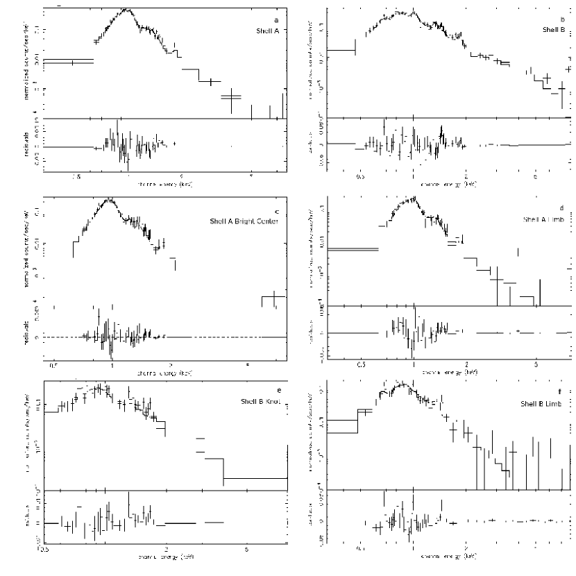
Figure 3: Spectral fits to Chandra ACIS data for: (a) Region 1, Shell A; (b) Region 2, Shell B; (c) Region 3, Shell A Bright Center; (d) Region 4, Shell A Limb; (e) Region 10, Shell B Bright Knot; and (f) Region 12, Shell B Limb.

References

- Anders & Grevesse (1989) Anders, E. & Grevesse, N. 1989, Geochimica et Cosmochimica Acta 53, 197
- Badenes et al. (2003) Badenes, C., Bravo, E., Borkowski, K. J., & Domínguez, I. 2003, ApJ, 593, 358
- Bodenheimer et al. (1984) Bodenheimer, P., Yorke, H. W., & Tenorio-Tagle, G. 1984, A&A, 138, 215
- Chu & Kennicutt (1988) Chu, Y.-H. & Kennicutt, R. C., Jr. 1988, AJ, 96, 1874
- Cox et al. (1999) Cox, D. P. et al. 1999, ApJ, 524, 179
- Gotthelf (2003) Gotthelf, E. V. 2003, ApJ, 591, 361
- Haberl & Pietsch (1999) Haberl, F. & Pietsch, W. 1999, A&AS, 139, 277
- Hendrick, Borkowski, & Reynolds (2003) Hendrick, S. P., Borkowski, K. J., & Reynolds, S. P. 2003, ApJ, 593, 370
- Hughes et al. (2003) Hughes, J. P. et al. 2003, ApJL, 582, 95
- Hughes et al. (1995) Hughes, J. P. et al. 1995, ApJL, 444, 81
- Ikeuchi (1978) Ikeuchi, S. 1978, PASJ, 30, 563
- Iwamoto et al. (1999) Iwamoto, K., Brachwitz, F., Nomoto, K., Kishimoto, N., Umeda, H., Hix, W. R., & Thielemann, F. 1999, ApJS, 125, 439
- Jones et al. (1979) Jones, E. M., Smith, B. W., Straka, W. C., Kodis, J. W., & Guitar, H. 1979, ApJ, 232, 129
- Kim et al. (2003) Kim, S., Staveley-Smith, L., Dopita, M. A., Sault, R. J., Freeman, K. C., Lee, Y., & Chu, Y.-H. 2003, ApJS, 148, 473
- Lewis et al. (2003) Lewis, K. T., Burrows, D. H., Hughes, J. P., Slane, P. O., Garmire, G. P., & Nousek, J. A. 2003, ApJ, 582, 770
- Masai (1994) Masai, K. 1994, ApJ, 437, 770
- Mathewson & Clarke (1973) Mathewson, D. S. & Clarke, J. N. 1973, ApJ, 180, 725
- Mathewson et al. (1983) Mathewson, D. S., Ford, V. L., Dopita, M. A., Tuohy, I. R., Long, K. S., & Helfand, D. J. 1983, ApJS, 51, 345
- Nishiuchi et al. (2001) Nishiuchi, M., Yokugawa, J., Koyama, K., & Hughes, J.P. 2001, PASJ, 53, 99
- Nomoto et al. (1997) Nomoto, K., et al. 1997, Nuclear Physics A, 616, 79c
- Park et al. (2003) Park, S. et al. 2003, ApJ, 586, 210
- Rho & Petre (1998) Rho, J. & Petre, R. 1998, ApJL, 503,167
- Rho et al. (1994) Rho, J., Petre, R., Schlegel, E. M., & Hester, J. J. 1994, ApJ, 430, 757
- Rohlfs et al. (1984) Rohlfs, K., Kretschmann, J., Siegman, B. C., & Feizinger, J. V. 1984, A&A, 137, 343
- Russel & Dopita (1992) Russel, S. C. & Dopita, M. A. 1992, ApJ, 384, 508
- Sarazin (1988) Sarazin, C. L. 1988, X-Ray Emission from Clusters of Galaxies (Cambridge: Cambridge Univ. Press)
- Schwering & Israel (1991) Schwering, P. B. W., & Israel, F. P. 1991, A&A, 246, 231
- Sedov (1959) Sedov, L. I. 1959, Similarity and Dimensional Methods in Mechanics (New York: Academic)
- Shelton, Kuntz, & Petre (2004) Shelton, R. L., Kuntz, K. D., & Petre, R. 2004, ApJ, 611, 906
- Shelton et al. (1999) Shelton, R. L. et al. 1999, ApJ, 524, 192
- Slavin & Cox (1992) Slavin, J. D. & Cox, D. P. 1992, ApJ, 392, 131
- Spitzer (1962) Spitzer, L. 1962, Physics of Fully Ionized Gases (New York: Interscience), p. 86
- Staveley-Smith et al. (2003) Staveley-Smith, L., Kim, S., Calabretta, M. R., Haynes, R. F., & Kesteven, M. J. 2003, MNRAS, 339, 87
- Sun et al. (2004) Sun, M., Seward, F. D., Smith, R. K., & Slane, P. O. 2004, ApJ, 605, 742
- van der Heyden et al. (2002) van der Heyden, K. J., Behar, E., Vink, J., Rasmussen, A. P., Kaastra, J. S., Bleeker, J. A. M., Kahn, S. M., & Mewe, R. 2002, A&A, 392, 955
- Velázquez et al. (2001) Velázquez, P. F. et al. 2001, RMxAC, 37, 87
- Weidemann (1990) Weidemann, V. 1990, ARA&A, 28, 103
- White & Long (1991) White, R. L., & Long, K. S. 1991, ApJ, 373, 543
- Williams et al. (1997) Williams, R. M., Chu, Y.-H., Dickel, J. R., Beyer, R., Petre, R., Smith, R. C., & Milne, D. K, 1997, ApJ, 480, 618
- Williams et al. (2005) Williams, R. M., Chu, Y.-H., Dickel, J. R., Gruendl, R. A., Seward, F. D., Guerrero, M. A. & Hobbs, G. 2005, ApJ, astro-ph/0504609
- Yusef-Zadeh et al. (2003) Yusef-Zadeh, F., Wardle, M., Rho, J., & Sakano, M. 2003, ApJ, 585, 319