Stochastic gravitational wave background from cold dark matter halos

Abstract

The current knowledge of cosmological structure formation suggests that Cold Dark Matter (CDM) halos possess a non-spherical density profile, implying that cosmic structures can be potential sources of gravitational waves via power transfer from scalar perturbations to tensor metric modes in the non-linear regime. By means of a previously developed mathematical formalism and a triaxial collapse model, we numerically estimate the stochastic gravitational-wave background generated by CDM halos during the fully non-linear stage of their evolution. Our results suggest that the energy density associated with this background is comparable to that produced by primordial tensor modes at frequencies $\nu\approx 10^{-18}-10^{-17}$Hz if the energy scale of inflation is $V^{1/4}\approx 1-2\times 10^{15}$ GeV, and that these gravitational waves could give rise to several cosmological effects, including secondary CMB anisotropy and polarization.

I Introduction

Sources of gravitational waves (GW) are commonly separated in two types: astrophysical and cosmological.

The first kind of sources can produce a stochastic background which provides interesting information on the distribution of compact objects at relatively low redshifts, such as star formation and supernova rates, black-hole growth mechanisms and other important phenomena. Such a background is generated by neutron stars, black holes and the associated binary systems, which emit in the frequency range $\nu_{e}\approx 10^{2}-10^{4}$Hz. (e.g Maggiore ; Ferrari et al. 1999 ), or by galactic merging of unresolved binary white dwarfs with frequencies in the range $\nu_{e}\approx 10^{-4}-10^{-2}$Hz Postnov97 ; Kosenko98 ; Schneider et al. 2000 ; Schneider et al. 2001 ; Farmer and Phinney 2003 .

Besides binary systems of super-massive black holes in the galaxy center, which could emit at $\nu_{e}\approx 10^{-4}$Hz, hence detectable by LISA (e.g. Ref. Grishchuk03 ), the principal example of gravitational waves of cosmological origin is represented by the relic radiation which has been generated by quantum fluctuations of the metric tensor during the inflationary era. The detection of this relic background would shed light on the physics of the very early Universe, since its strain amplitude is proportional to the square of the inflation energy scale. Primordial backgrounds can be generated by various mechanisms and are characterized by a large frequency interval which extends from a few $10^{-18}$ Hz to a few GHz, allowing their detection by markedly different ways of observation Maggiore .

One of the best strategies for detecting the relic gravitational radiation is to exploit the imprints it leaves on the Cosmic Microwave Background (CMB) temperature anisotropy and polarization Hu et al. 1998 ; reviews ; books . More specifically, the CMB photons are very sensitive to primordial GWs with frequencies $\approx 10^{-17}$Hz, which correspond to the comoving size of the Hubble radius at last scattering, when tensor metric modes, being damped by the horizon entering, produce the largest amount of temperature quadrupole anisotropy and, consequently, by Thomson scattering, the largest amount of polarization Pritchard&Kamionkowski04 . It may be shown that the curl component in the polarization pattern, commonly known as B-mode, is excited by vector and tensor cosmological perturbations only; therefore, if initial fluctuations are created very early, e.g. during inflation so that the vector growth is damped, primary B-modes can be produced only by tensor perturbations and, therefore, a possible detection will represent the incontrovertible proof of their existence Kamionkowski et al. 1997 ; Zaldarriaga&Seljak97 ; Seljak&Zaldarriaga97 .

Unfortunately, there are mechanisms that can produce secondary B-modes, the principal one being represented by the gravitational lensing, i.e. cosmic shear (CS) Bartelmann&Schneider01 , which distorts the primary CMB pattern, in particular converting E- into B-modes Zaldarriaga&Seljak98 . Luckily, although comparable, B-modes from primordial GW exhibit their peak at multipoles $l\approx 100$, corresponding to the degree scale, while, for lensed B-modes, the peak is at $l\approx 1000$, corresponding to the arcminute scale. Nonetheless, if the energy scale of inflation is $V^{1/4}\leq 2-4\times 10^{15}$GeV, the CS-induced curl is a foreground for the $l\approx 50-100$ primordial GW-induced B-polarization. This important contamination has to be removed in order to detect relic gravitational waves seljak_hirata_2004 . However, as suggested by WMAP measurements, early reionization should produce a large-angle bump in the primordial GW-induced B-modes, allowing a possibly easier detection, without confusion with the CS-induced curl Cabella&Kamionkowski04 .

Actually, besides gravitational lensing, for cosmological models which constantly seed fluctuations in the geometry, e.g. topological defects, vector metric perturbations can be huge and can produce non-negligible effects on the CMB photons as, in particular, B-mode polarization, unlike to what happens in inflationary models Turok et al. 1998 . On the other hand, no relevant contribution from these objects is indicated by the modern cosmological probes.

In the present paper, we are interested in the cosmological stochastic GW background produced by Cold Dark Matter (CDM) halos via power transfer from scalar and possible vector perturbations to tensor metric modes, during the strongly non-linear stage of their evolution CM . It differs from other cosmological backgrounds, as that produced during the mildly non-linear stage mm2 , since density and velocity fields can be, in this case, highly non-linear.

Since the non-linear evolution of CDM halos occurs on a cosmological timescale, the produced gravitational radiation may be relevant at frequencies comparable to those of the primordial GW which affect the CMB photons and, therefore, can produce secondary CMB anisotropy and polarization, expecially B-modes, that could represent a foreground for the detection of the relic radiation.

Moreover, as for the case of black holes and neutron stars, the analysis of the stochastic background produced by highly non-linear cosmic structures, could bring information on their distribution, evolution, shape and composition, shedding light on many open issues.

The plan of paper is as follows. In Sec. II we briefly outline the mathematical formalism and show the analytical formulas we use to estimate the GW output from CDM halos. In Sec. III we introduce the homogeneous ellipsoid dynamics as an approximation to the halo virialization and adopt the halo mass function of Ref. Sheth et al. 2001 to describe their distribution. In Sec. IV we explain the technique used for the numerical evaluation of the stochastic GW background, while in Sec. V we show and discuss our results. Finally Sec. VI contains our concluding remarks.

II Gravitational Radiation:
basic equations

The evolution of cosmological perturbations away from the linear regime is rich of several effects, such as the mode-mixing of different types of fluctuation, which not only implies that different Fourier modes influence each other, but also that density perturbations act as a source for curl vector modes and gravitational waves.

Accordingly, cosmic structures can generate tensor metric modes during the non-linear stage of their evolution and, in particular, this mechanism applies to dark matter halos around galaxies and galaxy clusters in the highly non-linear regime.

In the present paper, adopting the mathematical formalism developed in Ref. CM , we estimate the output in gravitational waves from cosmic structures, following their evolution from the linear to the highly non-linear level. More specifically, the evaluation of this gravitational radiation is possible on scales much larger than the Schwarzschild radius of collapsing bodies, by means of a “hybrid approximation” CM of the Einstein field equations, which mixes post-Newtonian (PN) (e.g. ch ; ch2 ; ch3 ; tomita3 ; tomita4 ; sa ; mt ) and second-order perturbative techniques (e.g. pyne ; mm ; mmb ; tomita ; mps ; tomita2 ) to deal with the perturbations of matter and geometry. This approach gives a more accurate description of gravitational waves generated by non-linear CDM structures than the standard second-order perturbation theory mm2 , which can only account for small deviations from the linear regime, or the Newtonian quadrupole radiation grav ; landau ; indeed, it upgrades the weak-field limit of Einstein equations to account for PN scalar and vector metric perturbations and for leading-order source terms of metric tensor modes. It provides, on small scales, a PN approximation to the source of gravitational radiation, and, on large scales, it converges to the first and second-order perturbative equations as obtained e.g. in Ref. mhm , but still describing, on all the cosmologically relevant scales, the dynamics of the involved CDM structures by means of the standard Newtonian Poisson, Euler and continuity equations (e.g. peebles )

$$\nabla^{2}\varphi=4\pi Ga^{2}\delta\rho\;,$$ (1)

$$\rho^{\prime}+3\mathcal{H}\rho+\partial_{\nu}(\rho\,v^{\nu})=0\;,$$ (2)

$$v_{\alpha}^{\prime}+\mathcal{H}v_{\alpha}+v_{\nu}\partial^{\nu}v_{\alpha}=-\partial_{\alpha}\varphi\;,$$ (3)

where $\varphi$ is the gravitational potential associated with the density perturbation, $\rho=\bar{\rho}+\delta\rho$ is the total matter density composed by the background matter density, $\bar{\rho}$, and the matter density perturbation, $\delta\rho$, and, finally, $\mathbf{v}$ is the peculiar velocity field associated to the CDM halos. Greek indices denote spatial components; we adopt conformal time $\eta$ and comoving coordinates $x^{\alpha}$, in the Poisson gauge, and assume that the Universe is spatially flat and filled with a cosmological constant $\Lambda$ and a pressureless fluid whose stress-energy tensor reads $T^{i}{}_{j}=\rho u^{i}u_{j}$ ($u^{i}u_{j}=-1$). Finally, $\mathcal{H}\equiv a^{\prime}/a$, where primes indicate differentiation with respect to $\eta$ and $a$ is the scale factor of the Universe which evolves according the Friedmann-Robertson-Walker background model.

Indeed, as the background cosmology, we have adopted a flat $\Lambda$CDM model with present baryon density given by $\Omega_{0\rm b}=4.318\times 10^{-2}$, dark and CDM energy density $\Omega_{0\Lambda}=0.7434$, $\Omega_{0\rm{CDM}}=0.2134$, Hubble constant $H_{0}=100h$ km/sec/Mpc where $h=0.7199$ and three massless neutrino species; the primordial perturbation spectrum is made by scalars only, normalized by $\sigma_{8}=\sigma(R=8\,h^{-1}\,\rm{Mpc})=0.9$, with spectral index $n_{s}=0.96$ Tegmark et al. 2004 ; Spergel et al. 2003 .

Accordingly to Ref. CM , in order to evaluate the stochastic background of gravitational radiation generated by CDM halos, we will exploit the formula expressing the solution of the inhomogeneous GW equation on scales well inside the Hubble horizon and in the so-called wave zone, which is

$$h^{\alpha}{}_{\beta}(\eta,\mathbf{x})=\frac{4G}{c^{4}}\frac{1}{ar}\mathcal{P}^{\alpha\;\;\mu}_{\;\;\nu\;\;\;\beta}\left[a^{3}\int d^{3}\tilde{x}\,\mathcal{R}^{\nu}_{\textrm{eff}\,\mu}\right]_{ret}\;,$$ (4)

where $r$ is the comoving distance between source and observer while the projection operator is given by $\mathcal{P}^{\alpha}{}_{\beta}\equiv\delta^{\alpha}{}_{\beta}-x^{\alpha}x_{\beta}/r^{2}$. Eq. (4) expresses the GW output $h^{\alpha}{}_{\beta}$ in terms of integrals over the source “stress distribution” $\mathcal{R}^{\alpha}_{\textrm{eff}\,\beta}$, given by

$$\mathcal{R}^{\alpha}_{\textrm{eff}\,\beta} =\rho\left(v^{\alpha}v_{\beta}-\frac{1}{3}v^{2}\,\delta^{\alpha}{}_{\beta}\right)+$$

$$+\frac{1}{4\pi Ga^{2}}\left(\partial^{\alpha}\varphi\,\partial_{\beta}\varphi-\frac{1}{3}\partial^{\nu}\varphi\,\partial_{\nu}\varphi\,\delta^{\alpha}{}_{\beta}\right)\;.$$ (5)

The subscript “ret” in Eq. (4) means that the quantity has to be evaluated at the retarded space-time point $\left(\eta-r/c,\mathbf{\tilde{x}}\right)$, i.e. at the source and at the emission time.

III The ellipsoidal collapse model

Recently, N-body simulations in CDM models have shown departure of the halo density profile from the spherical symmetry (e.g. Jing&Suto2000 ) and suggest a triaxial shape which seems to be confirmed by optical, X-ray and lensing observations of galaxy clusters (e.g. West ; Plionis et al.1991 ).

Consequently, according to the arguments in the previous Section, CDM halos are potential sources of gravitational radiation through power injection from the gravitational potential and peculiar velocity, especially during the highly non-linear stage of their evolution, when density contrasts and velocity fields can be strongly non-linear. Since the aim of this paper is to evaluate the stochastic GW background generated by a distribution of cosmic structures, in this Section we will describe the model adopted to approximate their dynamics and virialization.

III.1 The homogeneous ellipsoid dynamics

We will use the gravitational collapse of homogeneous ellipsoids as described in Ref. B&M , which developed a picture of cosmic structure formation that identifies virialized cosmological objects with peak patches in the initial Lagrangian space. These peaks represent overdensities in the initial Gaussian density field whose evolution is approximated by a homogeneous ellipsoid dynamics. Each perturbation evolves under the influence of its own gravity and under the external tidal field (generated by the surrounding matter) which, together with initial conditions, is chosen to reproduce the Zel’dovich approximation in the linear regime. Virialization is defined as the time when the third axis collapses and, following Ref. B&M , each axis is frozen once it has reached a freeze-out radius, chosen so that the density contrast at virialization, in the limit of spherical collapse, is the same as prescribed by the top-hat model.

The peculiar velocity field is conveniently described in the system identified by the three principal axes, characterized by three different scale factors $R_{\alpha}$ ($\alpha=1,2,3$); thus, inside the homogeneous ellipsoid, peculiar velocities may be written as

$$v_{\alpha}=\left(a\frac{\dot{R_{\alpha}}}{R_{\alpha}}-\dot{a}\right)x_{\alpha}\;,$$ (6)

where we are still adopting comoving coordinates but now time derivatives are with respect to the proper time $dt=a\,d\eta$.

The internal peculiar gravitational potential, still with respect to the principal-axis system, is given by (see Ref. B&M for details)

$$\varphi=\pi Ga^{2}\bar{\rho}\left[\sum_{\alpha=1}^{3}(\delta b_{\alpha}+2\lambda^{\prime}_{\alpha})x_{\alpha}^{2}\right]\;,$$ (7)

where $\delta\equiv\delta\rho/\bar{\rho}$ is the matter density contrast while the factors $b_{\alpha}$ are given by (see e.g. Refs. Chandra69 ; binney )

$$b_{\alpha}=R_{1}R_{2}R_{3}\int_{0}^{\infty}\frac{ds}{\left(R_{\alpha}^{2}+s\right)\sqrt{\left(R_{1}^{2}+s\right)\left(R_{2}^{2}+s\right)\left(R_{3}^{2}+s\right)}}$$ (8)

Finally, the coefficients $4\pi Ga^{2}\bar{\rho}\lambda^{\prime}_{\alpha}$ are the eigenvalues of the traceless external tidal tensor (proportional to the traceless part of the peak strain) for which a linear approximation is assumed B&M , imposing that it evolves through the same equations satisfied by the linear growth-factor of density fluctuations in the considered cosmological background.

After imposing the Zel’dovich approximation to fix the initial conditions on the proper ellipsoid axis lengths and their time derivatives, the evolution of an ellipsoidal perturbation is specified through the equations B&M

$$\frac{d^{2}R_{\alpha}}{dt^{2}}=\frac{\Lambda c^{2}}{3}R_{\alpha}-4\pi G\bar{\rho}R_{\alpha}\left(\frac{1}{3}+\frac{\delta}{3}+\frac{b_{\alpha}^{\prime}}{2}\delta+\lambda^{\prime}_{\alpha}\right)\;,$$ (9)

$$\frac{d^{2}a}{dt^{2}}=\left(-\frac{4\pi G}{3}\bar{\rho}+\frac{\Lambda c^{2}}{3}\right)a\;,$$ (10)

$$\rho R_{1}R_{2}R_{3}=\textrm{const}\;,$$ (11)

$$\bar{\rho}a^{3}=\textrm{const}\;,$$ (12)

where, in Eq. (9), $b_{\alpha}^{\prime}=b_{\alpha}-2/3$.

Eqs. (9)-(12) have been numerically integrated using a fourth-order Runge-Kutta scheme and the integrals (8) have been evaluated by means of the so-called Carlson’s elliptic function of the third kind.

Fig. 1 shows the axis evolution versus time of a homogeneous ellipsoid of mass $M=5\times 10^{15}M_{\odot}$ and initial overdensity $\delta(z_{i}=40)=6.4\times 10^{-2}$ at comoving distance $D=100\;{\rm Mpc}$ from the observer. The shape of the ellipsoid is the most probable in terms of the distribution of ellipticity and prolateness, to be defined in the next sub-Section. The evolution follows Eqs. (9-12) and the axis freezing out method suggested in Ref. B&M . Let us stress that, contrary to other ellipsoidal collapse schemes (e.g. W&S ), this model implies that virialization is reached when the third and not the first axis collapses, while the freezing out method avoids $\delta\longrightarrow\infty$.

In order to estimate the GW output by CDM cosmic structures, we insert Eqs. (6)-(7) in Eqs. (4)-(II) during the collapse of each homogeneous ellipsoid which represents, in our simulation, a CDM halo evolving towards virialization.

In Fig. 2 we show two of the three non-vanishing traceless source components generated by the halo collapse of Fig. 1. These components are evaluated with respect to the eigenframe of the ellipsoid principal axes at rest with respect to the expanding cosmological background; by performing a transverse projection, the gravitational waves in the observer frame are obtained. Actually, Fig. 2 represents these two components divided by $1+z=1/a(t)$, in order to separate the effects of the background expansion, included in Eq. (4), from the halo evolution itself.

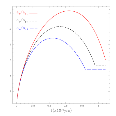
Figure 1: Evolution of the principal axis scale factors for the most probable ellipsoid of mass $M=5\times 10^{15}M_{\odot}$ and initial overdensity $\delta(z_{i}=40)=6.4\times 10^{-2}$, embedded in a flat $\Lambda$CDM universe, at distance $D=100\;{\rm Mpc}$ from the observer.

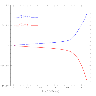
Figure 2: Two of the three non-vanishing traceless source components generated by the halo collapse of Fig. 1

III.2 The most probable ellipsoid and the halo mass function

Once the cosmological background model is fixed, the evolution of an ellipsoidal perturbation is determined by three parameters given by the three initial eigenvalues of what, in the Zel’dovich approximation, is called the deformation tensor, $d_{\alpha\beta}=(1/a^{2})\nabla^{2}_{\alpha}\nabla^{2}_{\beta}\varphi$; the latter are related to the initial ellipticity e, prolateness p and linear density contrast $\delta$ of the perturbation; those relations read Sheth et al. 2001

$$e=\frac{\lambda_{1}-\lambda_{3}}{2\delta}\;,$$ (13)

$$p=\frac{\lambda_{1}+\lambda_{3}-2\lambda_{2}}{2\delta}\;,$$ (14)

$$\delta=\lambda_{1}+\lambda_{2}+\lambda_{3}\;,$$ (15)

where the $\lambda_{\alpha}$ are the eigenvalues of $d_{\alpha\beta}$ with $\lambda_{1}\geq\lambda_{2}\geq\lambda_{3}$, which, if $\delta\geq 0$, implies $e\geq 0$ and $-e\leq p\leq e$.

For a Gaussian random density field, smoothed in real space with a top-hat filter of size $V=4\pi R^{3}/3$ and mass $M=4\pi\bar{\rho}R^{3}/3$, on average and for a given $\delta$ the prolateness is $p=0$; consequently, the most probable ellipticity is $e_{mp}=(\sigma/\delta)/\sqrt{5}$. Here $\sigma=\sigma(R)$ represents the linear rms value of the $\delta$ distribution Sheth et al. 2001 .

From these considerations and from the homogeneous ellipsoid collapse model as described in Ref. B&M , the authors of Ref. Sheth et al. 2001 have determined the shape of the moving barrier, i.e. the critical overdensity required for CDM structure virialization at redshift $z$; that is

$$B(\sigma^{2},z)=\sqrt{q}\delta_{sc}(z)\left[1+\beta(\alpha\nu)^{-\alpha}\right]\;,$$ (16)

where $\nu\equiv\left[\delta_{sc}(z)/\sigma(M)\right]^{2}$, $\delta_{sc}(z)$ is the critical overdensity required for spherical collapse at $z$ extrapolated using linear theory to the present time, and $\sigma$ is the linear rms value of the initial density fluctuation field also extrapolated to the present time. The parameters $\beta\approx 0.485$ and $\alpha\approx 0.615$ come from ellipsoidal dynamics and the value $q\approx 0.75$ comes from normalizing the model to simulations Sheth&Tormen 2002 .

Using Eq. (16) in the excursion set approach in order to obtain the distribution of the first crossings of the barrier by independent random walks, the authors of Refs. Sheth et al. 2001 ; Sheth&Tormen99 have derived the average comoving number density of halos of mass $M$, i.e. the so-called unconditional halo mass function

$$n(M,z)dM= \sqrt{\frac{2qA^{2}}{\pi}}\,\frac{\rho_{0}}{M^{2}}\,\frac{\delta_{sc}(z)}{\sigma(M)}\,\left[1+\left(\frac{\sigma(M)}{\sqrt{q}\delta_{sc}(z)}\right)^{2p}\right]$$

$$\times\left|\frac{{d}\ln\sigma}{{d}\ln M}\right|\,\exp\left(-\frac{q\delta_{sc}^{2}(z)}{2\sigma(M)^{2}}\right)dM\;,$$ (17)

where $\rho_{0}$ is the mean comoving cosmological mass density, while $p=0.3$ and $A=0.32218$. The Press-Schechter mass function is recovered for $q=1$, $p=0$ and $A=0.5$ Bond et al. 1991 .

In what follows, $\sigma(M)$ and $\delta_{sc}(z)$ are computed according to the formulas Kitayama&Suto ; Peacock&Dodds 1994 ; Sugiyama 1995

$$\sigma\propto(1+2.208m^{d}-0.7668m^{2d}+0.7949m^{3d})^{-2/(9d)}\;,$$ (18)

where $d=0.0873$, $m\equiv M(\Gamma h)^{2}/(10^{12}M_{\odot})$ and

$$\Gamma=\Omega_{0\rm m}h\exp\left[-\Omega_{0\rm b}\left(1+\sqrt{2h}/\Omega_{0\rm m}\right)\right]\;.$$ (19)

The quantities related to the density contrast are

$$\delta_{sc}(z)=\frac{\delta_{c}\,D_{+}(z=0)}{D_{+}(z)}\;,$$ (20)

$$\delta_{c}\approx\frac{3\,(12\pi)^{2/3}}{20}(1+0.0123\log_{10}\Omega_{\rm m})\;.$$ (21)

The linear growth factor of density fluctuations, normalized to unity at present, may be approximated as Carroll et al. 1992

$$D_{+}(z)=\frac{5\Omega_{\rm m}}{2(1+z)}\left[\Omega_{\rm m}^{4/7}-\Omega_{\Lambda}+\left(1+\frac{\Omega_{\rm m}}{2}\right)\left(1+\frac{\Omega_{\Lambda}}{70}\right)\right]^{-1}$$ (22)

where $\Omega_{\rm m}=\Omega_{0\rm m}(1+z)^{3}/E^{2}(z)$, $\Omega_{\Lambda}=\Omega_{0\Lambda}/E^{2}(z)$, and

$$E(z)=H(z)/H_{0}=\left[\Omega_{0\rm m}(1+z)^{3}+\Omega_{0\Lambda}\right]^{1/2}\;.$$ (23)

IV The stochastic GW background

In order to evaluate the GW output generated by a spatial distribution of CDM halos we will exploit Eq. (III.2) which provides a good fit to N-body simulations of structure clustering in a variety of cosmological models, at least over the redshift range $z=0-4$ Sheth et al. 2001 ; Sheth&Tormen 2002 ; Sheth&Tormen99 ; Kauffmann et al. 1999 ; Jenkins et al. 1998 .

For theoretical consistency, we have chosen to follow the same strategy adopted by Ref. Sheth et al. 2001 as described in the previous section. Therefore, in our numerical computation, we consider CDM structures over a mass range $M=5\times 10^{9}M_{\odot}-5\times 10^{15}M_{\odot}$, which virialize at redshifts from $z=0$ to $4$. Each of these structures is approximated by a homogeneous ellipsoidal perturbation with mass $M$, linear mass variance $\sigma^{2}(M)$ and critical linear density contrast $\delta(M,z)=B(\sigma^{2},z)$; in other words, every perturbation represents the most probable ellipsoid ($p=0$ and $e=e_{mp}$) of mass $M$ which collapses at redshift $z$.

Given the density contrast, the ellipticity and the prolateness, we then calculate the eigenvalues of the external tidal tensor, using Eqs.(13)-(15) and the relation $\lambda^{\prime}_{\alpha}=\lambda_{\alpha}-\delta/3$. Next, we linearly rescale all quantities to the initial redshift $z_{i}=40$, at which the ellipsoidal evolution of the density perturbation starts, following Eqs. (9)-(12). In fact, while the mass function provides the number of halos virializing at a given redshift (in our case $z=0-4$), the evolution of matter density perturbations, giving rise to these virialized objects, begins much before, i.e. at very high redshifts (in our case $z_{i}=40$). The initial conditions on the scale factor are given by the relation $a(z_{i})=1/(1+z_{i})$ and by the well-known Friedmann equations, while, as we have already anticipated, the initial conditions on the axis lengths and their time derivatives are specified by the Zel’dovich approximation setup

$$R_{\alpha}(z_{i})=a(z_{i})(1-\lambda_{\alpha})$$ (24)

and

$$\dot{R}_{\alpha}(z_{i})=H(z_{i})\left[R_{\alpha}(z_{i})-a(z_{i})f(z_{i})\lambda_{\alpha}\right]\;,$$ (25)

where $f(z)\approx\Omega_{\rm m}^{0.6}+\left(1/70\right)\left[1-1/2\Omega_{\rm m}\left(1+\Omega_{\rm m}\right)\right]$ is the growth rate of density fluctuations (e.g. Ref. Lahav ).

For each $M$ and $z$, using Eq. (4) and switching to the proper time $t$, we evaluate the two independent components of the gravitational radiation produced by a CDM halo, assuming that it is casually oriented and placed at a comoving distance $r(z)$ from the observer, where $z$ is the collapse redshift. In this way, we observe today the radiation emitted at the virialization time when, according to our ellipsoidal model, the GW output has the maximum value. Actually, adopting this strategy, we slightly underestimate the total GW background, since we do not take into account those CDM halos which are still away from virialization. Moreover it is noteworthy here that, in our approach, we have extrapolated Eq. (4) outside its range of validity. In fact, this formula holds on scales well inside the Hubble horizon and in the wave zone (i.e. at distances larger than both the characteristic wavelengths and the characteristic size of the source), while, as we previously noticed, CDM halos generate gravitational waves whose frequency is comparable with the inverse of the Hubble time. Nonetheless, as shown in the next Section, our results agree with several analytic approximations and previous works.

To account for all the directions of observation, we convert the two independent states $h^{\alpha}_{e{}\,\beta}(t)$ of tensor polarization from the frame associated with the ellipsoid principal axes to the observer frame, assuming that CDM structures emit in all directions and are uniformly distributed all around the observer. For this purpose, we use the relation $h^{\alpha}{}_{\beta}(t,\Omega)=R^{T\,\alpha}{}_{\nu}(\Omega)\,h^{\nu}_{e{}\,\mu}(t)\,R^{\mu}{}_{\beta}(\Omega)$ where $R^{\alpha}{}_{\beta}(\Omega)$ is the general form of the rotation matrix with $\psi=0$ Goldstein

$$R^{\alpha}{}_{\beta}(\Omega)\equiv\left(\begin{array}[]{ccc}\cos\phi&\sin\phi&0\cr-\cos\theta\sin\phi&\cos\theta\cos\phi&\sin\theta\cr\sin\theta\sin\phi&-\sin\theta\cos\phi&\cos\theta\end{array}\right)\;,$$

and the solid angle $\Omega\equiv\left(\theta,\phi\right)$ is defined following the conventions of Ref. Forward .

Since our aim is to estimate the energy density

$$\Omega_{\rm GW}(\nu)\approx\frac{2\pi^{2}}{3H_{0}^{2}}\nu^{3}\textrm{PSD}(\nu)$$ (26)

associated with the stochastic GW background at the observer (e.g. Ref. Maggiore ), we need to know the power spectral density PSD$(\nu)$, which one can obtain from the Parseval’s theorem as

$$\langle h^{\alpha}{}_{\nu}(t)h^{\nu}{}_{\beta}(t)\rangle=\int^{\infty}_{-\infty}d\nu\textrm{PSD}(\nu)\;.$$ (27)

That depends on the redshifted proper frequency $\nu=\nu_{e}/(1+z)$, where $\nu_{e}$ is the proper frequency at the emission time. In Eq. (27) angle brackets denote time averaging at a given spatial point.

Thus, we first numerically evaluate the PSD$(\nu,z,M,\Omega)$ of each individual component of $h^{\alpha}{}_{\beta}(t,\Omega)$ at each fixed value of $M$, $z$ and $\Omega$, then we average the calculated PSDs over all directions by integrating over the solid angle and dividing by $4\pi$ and, finally, we sum over the components in order to get a mean power spectral density PSD$(\nu,z,M)$ for every $z$ and $M$.

Since in our model each CDM halo is approximated by a most probable ellipsoid of mass $M$ which collapses at redshift $z$, we multiply each PSD$(\nu,z,M)$ by the number $dN(z,M)=n(z,M)dMdV$ of halos in the comoving volume $dV(z)=4c\,\pi r^{2}(z)dz/\left(a_{0}H(z)\right)$ where $c$ is the speed of light and $a_{0}\equiv 1$ is the present value of the scale factor. Finally, we insert the resulting quantity in the definition of the GW energy density Eq. (26) and integrate over all redshifts and masses to obtain the total $\Omega_{\rm GW}(\nu)$.

All the results are presented in the next section.

V Results

Our result concerning the GW output of each CDM halo, an example of which is given in Fig. 2, is consistent with previous works in this field Quilis98 ; Quilis00 . Moreover it is comparable to analytic approximations (e.g. grav ; Shapiro ) as

$$h\approx\frac{3\times 10^{-11}}{D/100\rm Mpc}\times\frac{GM\left(10^{15}\right)^{2/7}}{c^{2}L}\times\frac{M}{10^{15}M_{\odot}},$$ (28)

where $h$ represents the amplitude of a GW signal coming from a non-spherically symmetric collapsing object with characteristic size $L$ at distance $D$ from the observer.

It is worth noting that the produced gravitational radiation has a very long characteristic period, approximately given by the inverse of the halo evolution time, which, according to the ellipsoidal model, corresponds to frequencies of the order of $\nu\approx 10^{-18}$Hz. This excludes, therefore, any direct detection of a complete pulse, but still allows for the possibility of GW detection via secondary CMB anisotropy and polarization and via the “secular effect” discussed in Refs. Quilis98 ; Quilis00 . The latter takes place when a gravitational-wave crosses two testing particles; this induces a variation in their relative distance which increases in time, since this effect lasts for many years.

Actually, besides what stressed in the previous Section, there are other reasons for which the ellipsoidal collapse approximation to CDM halo virialization underestimates amplitude and frequency characterizing the GW background. In fact, using this approach, the evolution of cosmic structures is regarded as a continuous phenomenon which neglects merging effects and any possible features of variability that, according to Ref. Quilis98 , should be characterized by a dynamical frequency of the order of $\nu\approx 10^{-17}$Hz.

In Fig. 3 the main result of our paper is shown, i.e. the total energy density $\Omega_{\rm GW}(\nu)\approx 10^{-20}$, associated with the stochastic halo-induced GW background, as a function of the proper frequency $\nu$ at the observation. The total spectrum of the signal is composed by many single peaks which represent the contribution to the total background from each most probable halo weighted via the mass function at different redshifts. On the other hand, as the following discussion shows, these peaks are caused by the subset of structures leading to a non-negligible GW signal. In fact Eq. (4) shows that the GW amplitude is proportional to the inverse of the comoving distance, while, from the expression of the efficiency $\epsilon=GM/(c^{2}L)$ and the total radiated energy $E_{GW}=\epsilon Mc^{2}$, where $L$ represents the characteristic halo size at virialization, it follows that more massive objects give rise to higher values of the GW strain. This effect is also confirmed by numerical estimates of the power spectral density for different objects in the redshift range $0\leq z\leq 4$. In fact, masses of the order of $10^{8}-10^{9}M_{\odot}$, although weighted via the mass function in Eq. (III.2), contribute to $\Omega_{\rm GW}(\nu)$ by only a factor of orders of $10^{-30}-10^{-28}$; since the amplitude of the gravitational waves decreases with distance, the greater is the redshift $z$, the lower is their contribution. Thus only a few peaks are visible in Fig. 3 since the energy density produced by less massive structures is completely negligible with respect to the effect (of orders of $10^{-21}-10^{-20}$) of far more massive objects ($10^{14}-10^{15}M_{\odot}$) at low redshifts, $z\leq 1$.

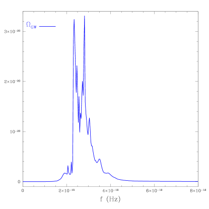
Figure 3: The total energy density $\Omega_{\rm GW}(\nu)$ associated with the stochastic GW background induced by CDM halos as a function of the proper frequency $\nu$ at observation.

Figure 4: Contribution to the total energy density $\Omega_{\rm GW}(\nu)$ by two most probable CDM halos of mass $5\times 10^{15}M_{\odot}$ placed at redshifts $z=0.025$ and $0.075$.

Consequently, the dominant contribution to the stochastic GW background is likely to be produced by CDM halos corresponding to nearby galaxies and galaxy clusters which contribute by several orders of magnitudes more than their substructures, although the latter are far more numerous. Indeed, in Fig. 4 we may look at the contribution to the total $\Omega_{\rm GW}(\nu)$ (see Fig. 3) by two most probable halos of mass $5\times 10^{15}M_{\odot}$, placed at redshifts $z=0.025$ and $0.075$. In its maximum height, the signal reaches about half of the corresponding value in Fig. 3. The remaining part of the signal is caused by many halos of comparable mass, as well as by those about one order of magnitude lighter, for which the mass decrease is compensated by the increase in the number. It is worth noting that the ellipsoidal collapse model introduces a three-peak pattern due to the freezing out method used to stop the axis collapse, which as a zero-th order approximation imposes stability at virialization, ignoring any residual dynamics. In the case of the specific geometrical configuration of the most probable ellipsoid considered in Fig. 4, this translates in two prominent peaks and a third negligible one. Actually, the residual dynamics at virialization would most probably imply a broadening of the spikes, decreasing the frequency splitting, possibly converging to a single peak for configurations close to sphericity.

Finally and most importantly, the quantity $h^{2}\Omega_{\rm GW}(\nu)\approx 10^{-20}$ is comparable to the energy density associated with the stochastic background induced by primordial GWs. In fact, if the energy scale of inflation is $V^{1/4}\approx 1-2\times 10^{15}\rm GeV$, the energy density associated with the primordial stochastic GW background, with a tensor spectral index $n_{T}\approx 0$, is $\approx 10^{-21}-10^{-17}$ for frequencies of the order of $10^{-18}-10^{-17}$ Hz (e.g Ref. Maggiore ).

VI Concluding remarks

In this work, we have estimated the GW background from cosmological tensor modes produced by the highly non-linear collapse of CDM density perturbations, i.e. generated during the strongly non-linear stage of CDM halo evolution.

We found that the signal is significant at very low frequencies, $\nu\approx 10^{-18}$ Hz, as a consequence of the cosmological time scales involved in the collapse of CDM halos. This signal appears as a broad peak made by the superposition of many impulses, all centered around frequencies of the order of $10^{-18}$ Hz. Most importantly, our results suggest that the signal is likely to be comparable to the primordial tensor power if inflation occurred at the GUT scale.

We want to stress that the homogeneous ellipsoidal collapse model, adopted to simulate CDM halo evolution and virialization, underestimates the frequency and amplitude of the emitted gravitational waves, since, at each redshift $z$, it does not take into account non-virialized objects and neglects variability features and merging effects that could enhance the anisotropic stress sourcing tensor modes, which are more sensible to the velocity field rather than to the peculiar gravitational potential. Consequently, the total energy density $\Omega_{\rm GW}(\nu)$ generated by cosmic structures could even be of one or two order of magnitudes greater and overcome the stochastic background associated with primordial gravitational waves at the same frequencies (see also results in Ref. Quilis00 ).

The CDM halo GW background could also produce a non-negligible contribution when considering the cosmological tensor-to-scalar ratio.

Due to the cosmological scales involved, and to the amplitude of the signal, it is reasonable to expect that these gravitational waves could affect the primary CMB anisotropies, contributing to the Integrated Sachs Wolfe (ISW) effect caused by the time evolution of cosmological perturbations between us and the last scattering surface. The stochastic GW background from CDM halos might boost the temperature anisotropies on large angular scales, where however the contribution from density fluctuations dominates. On the other hand, the produced temperature quadrupole can be scattered off by the free electrons of the intra-cluster and intra-galactic media, giving rise to secondary E and B polarization modes similarly to what happens for the primordial temperature quadrupole as described in Ref. Aghanim . These contributions have to be taken into account when performing a precise evaluation of the level of CMB polarization anisotropy expected for the forthcoming polarization oriented CMB probes, in particular for what concerns the B modes.

Most of these issues deserve a careful investigation in future works. Here we conclude stressing again our main results, suggesting that the amplitude of the stochastic GW background generated by CDM halos in their non-linear evolutionary phase is comparable or larger than the signal expected from the early universe in the inflationary scenario. We also remark that our findings are consistent with existing analytical approximations. The forthcoming steps are the improvement of the calculation of the source of the signal, making use of cosmological N-body simulations, as well as the computation of the induced CMB anisotropy in total intensity and polarization.

- (1) M. Maggiore, Phys. Rep. 331, 283 (2000).
- (2) V. Ferrari, S. Matarrese, R. Schneider, Mon. Not. Roy. Astron. Soc. 303, 258 (1999).
- (3) K. A. Postnov, in Proc. ”Particles and Cosmology”, 9th International Baksan School, 1997, [astro-ph/9706053].
- (4) D. I. Kosenko and K. A. Postnov, Astron. Astrophys. 336, 786 (1998).
- (5) R. Schneider, A. Ferrara, V. Ferrari, S. Matarrese, Mon. Not. Roy. Astron. Soc. 317, 385 (2000).
- (6) R. Schneider, V. Ferrari, S. Matarrese, S. F. Portegies Zwart, Mon. Not. Roy. Astron. Soc. 324, 797 (2001).
- (7) A. J. Farmer and E. S. Phinney, Mon. Not. Roy. Astron. Soc. 346, 1197 (2003).
- (8) L. P. Grishchuk, [arXiv:gr-qc/0305051].
- (9) W. HU, U. Seljak, M. White, M. Zaldarriaga, Phys. Rev. D 57, 3290 (1998).
- (10) M. Kamionkowski and A. Kosowsky, Ann. Rev. Nucl. Part. Sci. 49, 77 (1999); W. Hu and S. Dodelson, Ann. Rev. Astron. Astrophys. 40, 171 (2002).
- (11) S. Dodelson, Modern Cosmology (Academic Press, 2003); A. Liddle and D. H. Lyth, Cosmological Inflation and Large-Scale Structure (Cambridge University Press, 2000).
- (12) J. Pritchard and M. Kamionkowski, Annals Phys. 318, 2 (2005).
- (13) M. Kamionkowski, A. Kosowsky, A. Stebbins, Phys. Rev. D 55, 7368 (1997).
- (14) M. Zaldarriaga and U. Seljak, Phys. Rev. D 55, 1830 (1997).
- (15) U. Seljak and M. Zaldarriaga, Phys. Rev. Lett. 78, 2054 (1997).
- (16) M. Bartelmann and P. Schneider, Phys. Rept. 340, 291 (2001).
- (17) M. Zaldarriaga and U. Seljak, Phys. Rev. D 58, 023003 (1998).
- (18) U. Seljak and C. M. Hirata, Phys. Rev. D 69, 043005 (2004).
- (19) P. Cabella and M. Kamionkowski, Lectures given at the 2003 Villa Mondragone School of Gravitation and Cosmology: “The Polarization of the Cosmic Microwave Background,” Rome, Italy, September 6–11, 2003, [arXiv:astro-ph/0403392].
- (20) N. Turok, U. L. Pen, U. Seljak, Phys. Rev. D 58, 023506 (1998).
- (21) C. Carbone and S. Matarrese, Phys. Rev. D 71, 043508-1 (2005).
- (22) S. Matarrese and S. Mollerach, “The stochastic gravitational-wave background produced by non-linear cosmological perturbations”, in Proc. ”Some topics on General Relativity and Gravitational Radiation”, p.87, edited by J. A. Miralles, J. A. Morales, D. Saez, Editions Frontières, Paris, 1997, [arXiv:astro-ph/9705168].
- (23) R. K. Sheth, H. J. Mo, G. Tormen, Mon. Not. Roy. Astron. Soc. 323, 1 (2001).
- (24) S. Chandrasekhar, Astrophys. J. 142, 1488 (1965).
- (25) S. Chandrasekhar, Astrophys. J. 158, 45 (1969).
- (26) S. Chandrasekhar, Astrophys. J. 160, 153 (1970).
- (27) K. Tomita, Prog. Theor. Phys. 79, 258 (1988).
- (28) K. Tomita, Prog. Theor. Phys. 85, 1041 (1991).
- (29) M. Shibata, H. Asada, Prog. Theor. Phys. 94, 11 (1995).
- (30) S. Matarrese and D. Terranova, Mon. Not. Roy. Astron. Soc. 283, 400 (1996).
- (31) T. Pyne and S. Carroll, Phys. Rev. D 53, 2920 (1996).
- (32) S. Mollerach and S. Matarrese, Phys. Rev. D 56, 4494 (1997).
- (33) S. Matarrese, S. Mollerach and M. Bruni, Phys. Rev. D 58, 043504 (1998).
- (34) K. Tomita, Prog. Theor. Phys. 37, 831 (1967).
- (35) S. Matarrese, O. Pantano and D. Saez, Phys. Rev. Lett. 72, 320 (1994).
- (36) K. Tomita, Prog. Theor. Phys. 45, 1747 (1971); 47, 416 (1972).
- (37) C. W. Misner, K. S. Thorne and j. A. Wheeler, Gravitation, W. H. Freeman and Company, San Francisco (1973).
- (38) L. D. Landau and E. M. Lifshitz, The classical theory of fields, Pergamon Press, New York, (1975).
- (39) S. Mollerach, D. Harari and S. Matarrese, Phys. Rev. D 69, 063002 (2004).
- (40) P. J. E. Peebles, The Large–Scale Structure of the Universe, Princeton University Press, Princeton (1980).
- (41) M. Tegmark et al., Phys. Rev. D 69, 103501 (2004).
- (42) D. N. Spergel et al., Astrophys. J. Suppl. 148, 175 (2003).
- (43) Y. P. Jing and Y. Suto, Astrophys. J. 529, L69 (2000).
- (44) M. J. West, Astrophys. J. 347, 610 (1989).
- (45) M. Plionis, J. D. Barrow, C. S. Frenk, Mon. Not. Roy. Astron. Soc. 249, 662 (1991).
- (46) J. R. Bond and S. T. Myers, Astrophys. J. Suppl. Series 103, 1 (1996).
- (47) S. Chandrasekhar, Ellipsoidal Figures Equilibrium, Yale Univ. Press, New Haven, (1969).
- (48) J. Binney and S. Tremaine, Galactic Dynamics, Princeton Univ. Press, Princeton, (1987).
- (49) S. D. White and J. Silk, Astrophys. J. 231, 1 (1979).
- (50) R. K. Sheth and G. Tormen, Mon. Not. Roy. Astron. Soc. 329, 61 (2002).
- (51) R. K. Sheth and G. Tormen, Mon. Not. Roy. Astron. Soc. 308, 119 (1999).
- (52) J. R. Bond, S. Cole, G. Efstathiou, N. Kaiser, Astrophys. J. 379, 440 (1991).
- (53) T. Kitayama and Y. Suto, Astrophys. J. 469, 480 (1996).
- (54) J. A. Peacock and S. J. Dodds, Mon. Not. Roy. Astron. Soc. 267, 1020 (1994).
- (55) N. Sugiyiama, Astrophys. J. Suppl. Series 100, 281 (1995).
- (56) S. M. Carroll, W. H. Press, E. L. Turner, Annu. Rev. Astron. Astrophys. 30, 499 (1992).
- (57) G. Kauffmann, M. J. Colberg, A. Diaferio, S. D. M. White, Mon. Not. Roy. Astron. Soc. 303, 188 (1999).
- (58) A. Jenkins, C. S. Frenk, F. R. Pearce, P. A. Thomas, M. J. Colberg, S. D. M. White, H. M. P. Couchman, J. A. Peacock, G. Efstathiou, A. H. Nelson, Astrophys. J. 499, 20 (1998).
- (59) O. Lahav, P. B. Lilje, J. R. Primack, M. Rees, Mon. Not. Roy. Astron. Soc. 251, 128 (1991).
- (60) H. Goldstein, Classical Mechanics, Addison-Wesley, Cambridge, Mass., (1956).
- (61) R. L. Forward, Phys. Rev. D 17, 379 (1978).
- (62) V. Quilis, J. M. Ibanez and D. Saez, Astrophys. J. 501, L21 (1998).
- (63) V. Quilis, J. M. Ibanez and D. Saez, Astron. Astrophys. 353, 435 (2000).
- (64) S. L. Shapiro and S. A. Teukolsky, Black Holes, White Dwarfs ans Neutron Stars, John Wiley, New York, (1983).
- (65) G. C. Liu, A. da Silva, N. Aghanim, Astrophys. J. 621, 15 (2005).