An Improved Virial Estimate of Solar Active Region Energy

Abstract

The MHD virial theorem may be used to estimate the magnetic energy of active regions based on vector magnetic fields measured at the photosphere or chromosphere. However, the virial estimate depends on the measured vector magnetic field being force-free. Departure from force-freeness leads to an unknown systematic error in the virial energy estimate, and an origin dependence of the result. We present a method for estimating the systematic error by assuming that magnetic forces are confined to a thin layer near the photosphere. If vector magnetic field measurements are available at two levels in the low atmosphere (e.g. the photosphere and the chromosphere), the systematic error may be directly calculated using the observed horizontal and vertical field gradients, resulting in an energy estimate which is independent of the choice of origin. If (as is generally the case) measurements are available at only one level, the systematic error may be approximated using the observed horizontal field gradients together with a simple linear force-free model for the vertical field gradients. The resulting ‘improved’ virial energy estimate is independent of the choice of origin, but depends on the choice of the model for the vertical field gradients, i.e. the value of the linear force-free parameter $\alpha$. This procedure is demonstrated for five vector magnetograms, including a chromospheric magnetogram.

1 Introduction

There is considerable interest in the possibility of estimating energies for solar active regions from photospheric or chromospheric vector magnetic field measurements. Solar flares derive their energy from magnetic fields in active regions, and it is possible that reliable estimates of active region energy could be used to improve the accuracy of solar flare prediction. The problem is timely given the wealth of magnetic field measurements shortly to be available from the next generation of ground- and space-based vector magnetographs, in particular SOLIS (Keller, Harvey & Giampapa, 2003), and upcoming Solar Dynamics Observatory and Solar-B instruments.

One approach to the problem involves assuming the field is force-free, i.e. has a zero Lorentz force density ${\bf f}=\mu_{0}^{-1}(\nabla\times{\bf B})\times{\bf B}$ at and above the level of the measurements. In that case the simple form of the MHD virial theorem (Chandrasekhar 1961, chap. 13; Molodensky 1974)

$$\frac{1}{2\mu_{0}}\int_{z>0}B^{2}dV=\frac{1}{\mu_{0}}\int_{z=0}(B_{x}x+B_{y}y)B_{z}\,dxdy$$ (1)

applies. In this equation $z=0$ denotes the photosphere or chromosphere, which is approximated by a plane. In application to solar active regions, the interest is with the magnetic free energy, i.e. the energy associated with electric currents in the corona, rather than the total magnetic energy. This may be calculated by subtracting off the virial estimate $U$ for the potential field with the same $B_{z}$ distribution at $z=0$ (Low 1982).

There are many difficulties associated with applying Equation (1) to vector magnetic field measurements in solar active regions. The measured field values are noisy, in particular the transverse (to the line of sight) field values, and the errors may compromise the virial energy estimate (Klimchuk, Canfield & Rhoads 1992; Wheatland 2001). Error is also introduced by faults in the resolution of the 180 degree ambiguity in the direction of the transverse field (e.g. Metcalf 1994). A potentially more serious problem is that the magnetic field is not strictly force-free at the level of the photosphere, where most vector magnetic field measurements originate, so the basic assumption underlying Equation (1) is not met. A related point is that the right hand side of Equation (1) is dependent on the choice of the origin of the co-ordinate system, unless the net horizontal Lorentz force on the volume vanishes. Specifically, if we denote the integral on the right hand side of Equation (1) by $W_{0}$, then if the origin is changed to $(x_{0},y_{0})$, the integral becomes

$$W_{0}^{\prime}=W_{0}+x_{0}F_{x}+y_{0}F_{y},$$ (2)

where

$$F_{x}=\int_{z>0}f_{x}\,dV=-\frac{1}{\mu_{0}}\int_{z=0}B_{x}B_{z}\,dxdy$$ (3)

and

$$F_{y}=\int_{z>0}f_{y}\,dV=-\frac{1}{\mu_{0}}\int_{z=0}B_{y}B_{z}\,dxdy$$ (4)

are the net horizontal Lorentz forces on the volume (Molodenskii 1969; Aly 1984). Hence for non-zero $F_{x}$ or $F_{y}$ there is no unique virial energy estimate.

Equation (1) was first applied to photospheric vector magnetic field data by Gary, Moore & Hagyard (1987) and Sakurai (1987). Gary, Moore & Hagyard (1987) found $W_{0}-U$ to be of order $10^{25}\,{\rm J}$ for one active region. Although they did not state the choice of origin for this result, they investigated the influence of random errors in individual field measurements on the potential component of the energy, and concluded that the non-potential component was $3\sigma$ above the noise. Sakurai (1987) was less successful: for 120 vector magnetograms he found $(W_{0}-U)/U\approx 0.085\pm 0.81$. However, Sakurai did not mention the choice of origin. Klimchuk, Canfield & Rhoads (1992) investigated the influence of polarisation measurement errors on energy estimates made using Equation (1), and concluded that the detection of non-potential energy may be possible for the most energetic active regions. However, they also did not consider the problem of the origin-dependence of the estimates.

Metcalf et al. (1995) appear to be the first authors to explicitly consider the consequence of non-zero Lorentz forces for the practical application of the virial theorem. They examined the height dependence of net Lorentz forces for an active region by making observations using the Mees Solar Observatory Stokes Polarimeter at different offsets from the center of the chromospheric Na I $\lambda$5896 line, thereby sampling different heights in the atmosphere. They found that the forces become small about 500 km above the photosphere. They applied Equation (1) to the field determined at each height, and averaged over a number of choices of origin within the field of view. McClymont, Jiao & Mikic (1997) subsequently pointed out that the virial energy estimate (1) is dimensionally of order $B^{2}L^{3}/\mu_{0}$, where $B$ is the average field strength and $L$ is the horizontal extent of the active region, whereas the true energy is of order $B^{2}L^{2}H/\mu_{0}$, where $H<L$ is the scale height of the field. This implies that there is substantial cancellation in the virial integral. It follows from Equation (2) that if $F_{i}L/(B^{2}L^{3}/\mu_{0})$ is of order $H/L$ (for $i=x,y$), then the change in the virial energy associated with moving the origin across the field of view is comparable to the true energy. McClymont, Jiao & Mikic (1997) gave an example of applying Equation (1) to a particular active region, and by varying the origin over the field of view found total energy estimates ranging from $1.23\times 10^{26}\,{\rm J}$ to $1.92\times 10^{26}\,{\rm J}$, compared with the (unique) potential field energy $1.65\times 10^{26}\,{\rm J}$. They concluded that “any virial theorem estimate of the free energy is meaningless”, and suggested that it is better to calculate a three dimensional magnetic field from boundary values and estimate its energy. However, calculating a realistic model of the field (e.g. a nonlinear force-free model) based on observed boundary values is itself a challenging problem. Other authors have also estimated net Lorentz forces from vector magnetic field data. Based on 12 photospheric vector magnetograms, Moon et al. (2002) reported downward Lorentz forces of order $0.06-0.32$ times the magnetic pressure force, with a median value of 0.13. More recently Georgoulis & LaBonte (2004) estimated net vertical Lorentz forces for a number of photospheric vector magnetograms using a novel technique and reported large values.

The Mees Solar Observatory Imaging Vector Magnetograph is now routinely producing chromospheric magnetograms using the Na I $\lambda$5896 line, which as noted above is formed at a height in the atmosphere which is close to being force free (Metcalf et al. 1995). Recently Metcalf, Leka & Mickey (2005) calculated total and free magnetic energies for active region 10486 (which produced a number of the large ‘Halloween flares’ of October-November 2003) using chromospheric vector magnetograms from Mees. They were unable to identify a change in energy associated with the X10 flare of 29 October 2003, but they determined the free energy of the active region at three different times to be of order $10^{26}\,{\rm J}$. They also found the field to be almost force free, with ratios of the net horizontal Lorentz forces to the net magnetic pressure force of order $0.01$. Following Metcalf et al. (1995), Metcalf, Leka & Mickey applied Equation (1) with a ‘pseudo-Monte Carlo’ procedure involving choosing many different origins within the field of view and averaging the results. Their quoted errors are standard deviations corresponding to this procedure.

In this paper we identify the source of the origin dependence of virial energy estimates of the total magnetic energy as the neglect of additional terms involving volume integrals of spatial moments of the Lorentz force density. We point out that the missing terms may be calculated in straightforward ways assuming (as is observed) that the Lorentz forces are confined to a thin layer above the photosphere. If measurements of the vector magnetic field are available at two heights in the low atmosphere, e.g. at the photosphere and chromosphere, then the missing terms may be calculated directly using observed horizontal and vertical field gradients. It is more common to have measurements at a single height, for example from a photospheric vector magnetograph. In this case the missing terms may be approximated using the observed horizontal field gradients together with vertical field gradients from a simple linear force-free model. The result is termed an ‘improved’ virial energy estimate. By construction it is independent of the choice of origin, although it depends on the choice of the model for the vertical field gradients. We also investigate the pseudo-Monte Carlo method of averaging Equation (1) over choices of origin within the field of view. We show that this method is expected to give reliable estimates of the magnetic energy if the Lorentz forces are approximately uniformly distributed across the region of interest. More generally the distribution of Lorentz forces needs to be modelled, for example using the methods outlined here. We further show that the pseudo-Monte Carlo procedure is equivalent to the simple virial estimate with the origin at the center of the field of view, and we obtain an analytic expression for the standard deviation associated with the averaging procedure. The improved virial method is then demonstrated by application to five sets of vector magnetic field data, including a chromospheric vector magnetogram.

The layout of the paper is as follows. In section 2 the origin dependence of the virial integral is discussed, and the improved virial method is outlined. In section 3 the improved method is applied to vector magnetograms, and in section 4 the results are discussed. The Appendix presents analytic results corresponding to the pseudo-Monte Carlo procedure.

2 Method

2.1 The origin dependence of the virial integral

A form of the virial theorem taking into account the possibility of non-zero Lorentz forces is (Molodenskii 1969)

$$\frac{1}{2\mu_{0}}\int_{z>0}B^{2}\,dV=\frac{1}{\mu_{0}}\int_{z=0}(B_{x}x+B_{y}y)B_{z}\,dxdy+\int_{z>0}{\bf r}\cdot{\bf f}\,dV,$$ (5)

where ${\bf f}$ is the Lorentz force density. This expression may be rewritten as

$$W=W_{0}+W_{1},$$ (6)

where $W$ denotes the total magnetic energy, $W_{0}$ is the simple virial estimate appearing on the right hand side of Equation (1), and $W_{1}$ is the final integral in Equation (5). This latter term may be written

$$W_{1}=\langle x\rangle F_{x}+\langle y\rangle F_{y}+\langle z\rangle F_{z},$$ (7)

where

$$\langle x\rangle=\left.\int_{z>0}f_{x}x\,dV\right/\int_{z>0}f_{x}\,dV,$$ (8)

$$\langle y\rangle=\left.\int_{z>0}f_{y}y\,dV\right/\int_{z>0}f_{y}\,dV,$$ (9)

and

$$\langle z\rangle=\left.\int_{z>0}f_{z}z\,dV\right/\int_{z>0}f_{z}\,dV$$ (10)

are Lorentz force-weighted average positions. There is observational evidence that the Lorentz forces are confined to a narrow layer close to the photosphere (Metcalf et al. 1995). Hence we make the approximations

$$\int_{z>0}f_{x}x\,dV \approx \Delta z\int_{z=0}f_{x}x\,dxdy,$$

$$\int_{z>0}f_{x}\,dV \approx \Delta z\int_{z=0}f_{x}\,dxdy,$$ (11)

where $\Delta z$ is the thickness of the forcing layer, and similarly for the integrals in Equations (9) and (10). This leads to

$$\langle x\rangle\approx\left.\int_{z=0}f_{x}x\,dxdy\right/\int_{z=0}f_{x}\,dxdy,$$ (12)

$$\langle y\rangle\approx\left.\int_{z=0}f_{y}y\,dxdy\right/\int_{z=0}f_{y}\,dxdy,$$ (13)

and $\langle z\rangle=0$.

For non-zero Lorentz forces, $W_{1}$ will (in general) be non-zero. The term $W_{1}$ then represents a systematic error in the simple estimate (1) of the magnetic energy. In general this term cannot be estimated precisely by considering how $W_{0}$ changes under various changes of origin, e.g. by moving the origin within the field of view (Metcalf et al. 1995; Metcalf, Leka & Mickey 2005). From Equation (2), the change in $W_{0}$ due to shifting the origin depends only on the net Lorentz force components $F_{x}$ and $F_{y}$, which may be estimated using Equations (3) and (4). However, the term $W_{1}$ depends on moments of the components of the Lorentz forces, which in general cannot be calculated from the net Lorentz forces alone.

It is easy to see that by replacing $x$ and $y$ in Equation (8) by $x-x_{0}$ and $y-y_{0}$, the terms $\langle x\rangle$ and $\langle y\rangle$ are replaced by

$$\langle x\rangle^{\prime}=\langle x\rangle-x_{0},\quad{\rm and}\quad\langle y\rangle^{\prime}=\langle y\rangle-y_{0}.$$ (14)

Hence under this change of origin $W_{1}$ becomes

$$W^{\prime}_{1}=W_{1}-x_{0}F_{x}-y_{0}F_{y}.$$ (15)

Combining this with Equation (2), we see that $W=W_{0}+W_{1}$ is invariant under the change of origin, as required. In changing the origin, both $W_{0}$ and $W_{1}$ change by the same amount, but the change gives no information about the true size of $W_{1}$.

It is straightforward to calculate the result of the pseudo-Monte Carlo method of Metcalf, Leka & Mickey (2005) in which $W_{0}$ is averaged over all choices of origin within the field of view, subject to the approximation that the measured magnetic field lies in a plane tangent to the photosphere at the center of the field of view (see e.g. Gary & Hagyard 1990). If we denote the virial estimate with the origin corresponding to the lower left hand corner of the magnetogram by $W_{0}$, then from Equation (2), the estimate with a choice of origin translated by $(x_{0},y_{0})$ in the heliographic plane is $W_{0}^{\prime}=W_{0}+x_{0}F_{x}+y_{0}F_{y}$. We require the average of $W_{0}^{\prime}$ over all choices of $x_{0}$ and $y_{0}$ within the field of view, which may be written

$$\overline{W_{0}^{\prime}}=W_{0}+\overline{x}_{0}F_{x}+\overline{y}_{0}F_{y},$$ (16)

where $\overline{x}_{0}$ denotes the average of $x_{0}$, and similarly for $\overline{y}_{0}$. In the Appendix it is shown that the average position $(\overline{x}_{0},\overline{y}_{0})$ corresponds to the center of the image plane field of view. Comparing Equations (2) and (16) it follows that $\overline{W_{0}^{\prime}}$ is equal to the virial integral with the origin at the center of the image plane field of view. The Appendix provides analytic expressions for $\overline{x}_{0}$ and $\overline{y}_{0}$, as well as an expression for the standard deviation associated with averaging $W_{0}^{\prime}$ over all choices of origin in the field of view, in terms of $F_{x}$, $F_{y}$, and the geometry.

From Equations (12), (13), and (A2) it follows that if $f_{x}$ and $f_{y}$ are constant in the plane $z=0$, we have $\langle x\rangle=\overline{x}_{0}$ and $\langle y\rangle=\overline{y}_{0}$. In other words if the Lorentz forces are uniform, the Lorentz-force weighted average positions coincide with the average positions. In this case $W_{1}=\overline{x}_{0}F_{x}+\overline{y}_{0}F_{y}$, so $W=W_{0}+\overline{x}_{0}F_{x}+\overline{y}_{0}F_{y}=\overline{W_{0}^{\prime}}$, i.e. the pseudo-Monte Carlo method gives the correct answer. Somewhat more generally, if the Lorentz forces are approximately uniformly distributed over the region of interest, the simple form of the virial theorem with the origin at the center of the field of view gives approximately the correct answer for the total energy.

It is more realistic to assume that the forces are non-uniformly distributed, and in that case $\overline{W_{0}^{\prime}}$ will not give the correct energy. In the next section we consider how to model the Lorentz forces $f_{x}$ and $f_{y}$ over the field of view to give a more accurate, and origin-independent, estimate of the total magnetic energy.

2.2 Estimating $f_{x}$ and $f_{y}$ in the plane $z=0$

The basic idea is to approximate $f_{x}$ and $f_{y}$ in the plane $z=0$ based on available field gradients, and modelling where necessary. If the approximate versions of $f_{x}$ and $f_{y}$ are denoted $\widetilde{f}_{x}$ and $\widetilde{f}_{y}$, then we can write for our estimates of the force-weighted positions

$$\widetilde{\langle x\rangle}=\left.\int_{z=0}\widetilde{f}_{x}x\,dxdy\right/\int_{z=0}\widetilde{f}_{x}\,dxdy$$ (17)

and

$$\widetilde{\langle y\rangle}=\left.\int_{z=0}\widetilde{f}_{y}y\,dxdy\right/\int_{z=0}\widetilde{f}_{y}\,dxdy,$$ (18)

and our estimate of the total energy becomes

$$\widetilde{W}=W_{0}+\widetilde{\langle x\rangle}F_{x}+\widetilde{\langle y\rangle}F_{y}.$$ (19)

We note in passing that the definitions Equations (17) and (18) of the force-weighted positions require the integrals in the denominators to be non-zero.

The reason for writing the energy in this way is that $\widetilde{\langle x\rangle}$ and $\widetilde{\langle y\rangle}$ have the same behavior under a change of origin as the exact expressions $\langle x\rangle$ and $\langle y\rangle$. Specifically, if the origin is changed to $(x_{0},y_{0})$, then from Equations (17) and (18) the force-weighted positions change to

$$\widetilde{\langle x\rangle}^{\prime}=\widetilde{\langle x\rangle}-x_{0},\quad{\rm and}\quad\widetilde{\langle y\rangle}^{\prime}=\widetilde{\langle y\rangle}-y_{0}.$$ (20)

Combining this with Equations (2) and (19), it follows that $\widetilde{W}$ is independent of the choice of origin. Hence our procedure ensures an estimate of the energy which is origin independent, a result which holds for any choices of $\widetilde{f}_{x}$ and $\widetilde{f}_{y}$. Of course, the value of $\widetilde{W}$ will depend on the specific choices. Hence we have gained origin independence, i.e. a unique value, at the expense of model dependence.

The Lorentz force density components $f_{x}$ and $f_{y}$ may be written from their definition as

$$f_{x}=\frac{1}{\mu_{0}}\left[B_{z}\left(\frac{\partial B_{x}}{\partial z}-\frac{\partial B_{z}}{\partial x}\right)-B_{y}\left(\frac{\partial B_{y}}{\partial x}-\frac{\partial B_{x}}{\partial y}\right)\right]$$ (21)

and

$$f_{y}=\frac{1}{\mu_{0}}\left[B_{x}\left(\frac{\partial B_{y}}{\partial x}-\frac{\partial B_{x}}{\partial y}\right)-B_{z}\left(\frac{\partial B_{z}}{\partial y}-\frac{\partial B_{y}}{\partial z}\right)\right].$$ (22)

The horizontal derivatives in these expressions may be estimated from vector magnetic field data. If simultaneous measurements are available at two heights in the low atmosphere (e.g. at the photosphere and chromosphere), then the vertical derivatives may also be estimated from the data. However, measurements typically are available at only one height. In that case the vertical derivatives are not specified by the data, and we adopt a procedure of modelling the derivatives based on available information. Specifically, we use vertical derivatives from a linear force-free model for the field. (Note that if the horizontal components of the linear force-free field match the observed $B_{x}$ and $B_{y}$ everywhere then $f_{x}=f_{y}=0$.) This procedure is similar to a common practice in the resolution of the 180 degree ambiguity, where the value of ${\rm div}\,{\bf B}$ is estimated from the data locally using linear force-free estimates of vertical gradients (e.g. Metcalf 1994).

The linear force-free model is defined by ${\rm curl}\,{\bf B}=\alpha{\bf B}$, where $\alpha$ is the force-free constant. The $x$- and $y$-components of this equation give the expressions for the vertical gradients

$$\frac{\partial B_{y}}{\partial z}=-\alpha B_{x}+\frac{\partial B_{z}}{\partial y}\quad{\rm and}\quad\frac{\partial B_{x}}{\partial z}=\alpha B_{y}+\frac{\partial B_{z}}{\partial x}.$$ (23)

Combining Equations (21), (22) and (23) gives the model forms for $f_{x}$ and $f_{y}$:

$$\widetilde{f}_{x}(\alpha)=\frac{1}{\mu_{0}}B_{y}\left(\alpha B_{z}-\mu_{0}J_{z}\right)$$ (24)

and

$$\widetilde{f}_{y}(\alpha)=\frac{1}{\mu_{0}}B_{x}\left(\mu_{0}J_{z}-\alpha B_{z}\right),$$ (25)

where

$$J_{z}=\frac{1}{\mu_{0}}\left(\frac{\partial B_{y}}{\partial x}-\frac{\partial B_{x}}{\partial y}\right)$$ (26)

is the vertical current density. The form of these expressions makes clear the point that the estimates of the horizontal Lorentz forces will be zero if the observed horizontal gradients match those of a force-free field, i.e. if $J_{z}=\alpha B_{z}/\mu_{0}$ is satisfied everywhere.

Equations (17), (18), and (19) together with (24) and (25) provide an ‘improved’ virial energy estimate $\widetilde{W}(\alpha)$, which is independent of the choice of origin, but which depends on the choice of the parameter $\alpha$. In Section 3 this estimate is evaluated for five vector magnetograms.

There are several sources of uncertainty in the improved virial estimate. There is uncertainty associated with the modeling (i.e. the use of linear force-free fields to approximate the vertical gradients), and with the approximations inherent in Equations (12) and (13). These uncertainties are hard to quantify. There is also error in the energy estimate due to errors in the vector magnetic field measurements, and due to the uncertainty in the choice of $\alpha$. In Section 3 we will attempt to quantify these latter uncertainties, to give some measure of how reliable the estimate is.

A practical point to note in applying these formulae is that the horizontal derivatives and integrals are with respect to heliographic co-ordinates $(x,y)$. For data from vector magnetograms, these points form a non-uniform, non-Cartesian grid specified by the projection of points in the magnetograph field of view onto the photosphere or chromosphere. The evaluation of derivatives and integrals is simplified by working with co-ordinates in the image plane, which are uniformly spaced. In the calculations in this paper we follow this practice, using the approximation that heliographic co-ordinates lie on a plane tangent to the solar surface at the center of the region of interest. In that case there is a simple linear transformation between the co-ordinate systems (e.g. Gary & Hagyard 1990; Venkatakrishnan & Gary 1990).

3 Application to vector magnetograms

The improved virial method was applied to five vector magnetograms from the Mees Solar Observatory Imaging Vector Magnetograph (IVM). Four are photospheric magnetograms: NOAA active region 9077 observed on 14 July 2000 at 16:33UT (this is the Bastille Day 2000 flare region, observed after the flare occurred); NOAA AR 10306 observed on 13 March 2003 at 17:14UT; NOAA AR 10386 observed on 20 June 2003 at 16:38UT; and NOAA AR 10397 observed on 1 July 2003 at 18:18UT. These four magnetograms provide a typical selection of data. The fifth dataset is one of the chromospheric vector magnetograms previously studied by Metcalf, Leka & Mickey (2005): NOAA AR 10486, observed on 29 October 2003 at 18:46UT. In each case the data correspond to measurements at one height in the solar atmosphere, and so we follow the procedure of modelling vertical derivatives using a linear force-free model.

The IVM has 512 by 512 pixels with 0.55 arc second size, resulting in a field of view of about 4.7 arc minutes. (The corresponding projected distance at 1 AU is $L\approx 2.0\times 10^{8}\,{\rm m}$.) Details of the processing of IVM photospheric data are given in LaBonte, Mickey & Leka (1999), and further details of the chromospheric magnetogram are given in Metcalf, Leka & Mickey (2005). In each case the resolution of the azimuthal ambiguity was performed using the ‘minimum energy’ method (Metcalf 1994).

For each magnetogram the following procedure was followed. First the fractional flux balance $\phi$ (the ratio of signed to unsigned magnetic flux) was evaluated. Next the energy $U$ of a potential field with the given boundary values $B_{z}$ was determined from the virial theorem using the Fourier transform potential field solution (Alissandrakis 1981), with the Fourier transforms being performed with respect to image co-ordinates (see Venkatakrishnan & Gary 1989). The simple virial estimate $W_{0}$ of Equation (1) was then evaluated, with the origin correponding to the lower left hand corner of the magnetogram (this choice of origin is taken as the default for all origin-dependent terms). The forces $F_{x}$ and $F_{y}$ were also evaluated, together with the reference magnetic pressure force (Aly 1989)

$$F_{0}\equiv\frac{1}{2\mu_{0}}\int_{z=0}(B_{x}^{2}+B_{y}^{2}+B_{z}^{2})\,dxdy.$$ (27)

Then the estimate $\overline{W}_{0}=W_{0}+\overline{x}_{0}F_{x}+\overline{y}_{0}F_{y}$ corresponding to the pseudo-Monte Carlo method of Metcalf, Leka & Mickey (1995) was calculated using Equation (A).

Next the parameter $\alpha$ was determined by minimizing the least squares difference between the observed horizontal field and the horizontal field associated with the linear force-free field (Leka & Skumanich 1999). An uncertainty $\sigma_{\alpha}$ was also calculated, based on the variation in the goodness of fit as a function of $\alpha$. The functions $\widetilde{f}_{x}(\alpha)$ and $\widetilde{f}_{y}(\alpha)$ were then evaluated at each gridpoint based on estimates of the horizontal derivatives from differencing, with the differencing performed in image plane co-ordinates (Gary & Hagyard 1990). The resulting values were subject to $3\times 3$ median smoothing to remove spikes. The force-weighted positions $\widetilde{\langle x\rangle}(\alpha)$ and $\widetilde{\langle y\rangle}(\alpha)$ were then evaluated, and the improved virial energy $\widetilde{W}(\alpha)$ and the corresponding estimate of the free energy $\widetilde{W}(\alpha)-U$ were calculated.

Finally two uncertainties were numerically evaluated. The error in the energy estimate due to the the errors in the field measurements was estimated by a Monte Carlo procedure involving 100 evaluations of the improved virial energy estimate, with the field values $B_{x}$, $B_{y}$, and $B_{z}$ subject to random Gaussian perturbations at each evaluation according to the estimated errors in the measurements. The standard deviation of the 100 estimates was taken as the estimate of the uncertainty due to the field measurements, and this estimate is denoted $\sigma({\bf B})$. The second uncertainty considered is the error in the estimate due to the uncertainty $\sigma_{\alpha}$ in the value of the force-free parameter $\alpha$. It is straightforward to propagate the uncertainty in $\alpha$ through to an uncertainty in $\widetilde{W}(\alpha)$ using Equations (17), (18), (19), (24) and (25), and the resulting estimate is denoted $\sigma(\alpha)$. The two uncertainties were not combined because they describe quite different things.

The results are presented in Table 1. For AR 9077, the improved virial estimate $\widetilde{W}_{0}(\alpha)-U\approx-2.0\times 10^{25}\,{\rm J}$ is negative, which is unphysical. However, for this case the estimate $\overline{W}_{0}-U\approx-4.6\times 10^{25}\,{\rm J}$ — corresponding to the pseudo-Monte Carlo method — is also negative. The estimated uncertainties $\sigma(\alpha)$ and $\sigma({\bf B})$ do not account for the negative value, and hence in this case a physically meaningful estimate for the free energy is not obtained. For AR 10306, the improved virial estimate $\widetilde{W}_{0}(\alpha)-U\approx 5.8\times 10^{25}$ is slightly smaller than the pseudo-Monte Carlo estimate. However, the estimated uncertainties are both comparable to the improved virial estimate. For AR 10386, the improved virial estimate $\widetilde{W}_{0}(\alpha)-U\approx 2.3\times 10^{25}\,{\rm J}$ is somewhat smaller than the pseudo-Monte Carlo estimate, whilst $\sigma(\alpha)$ is larger than the improved virial estimate. For AR 10397, the improved virial estimate $\widetilde{W}_{0}(\alpha)-U\approx 4.5\times 10^{26}\,{\rm J}$ is very large, even larger than the pseudo-Monte Carlo estimate. In this case the uncertainties are somewhat smaller than the improved virial estimate. For the chromospheric magnetogram (AR 10486) the improved virial estimate $\widetilde{W}_{0}(\alpha)-U\approx 2.6\times 10^{26}\,{\rm J}$ is very similar to the pseudo-Monte Carlo value, and the estimated uncertainties are an order of magnitude smaller. These results suggest that a meaningful energy estimate is being obtained in this case.

The results for the photospheric magnetograms are mixed. There is once instance (AR 9077) of a negative free energy estimate, and this is for a large, apparently non-potential active region. For all of the photospheric magnetograms the estimated uncertainties are large, and in particular the uncertainties $\sigma(\alpha)$ associated with the model for the vertical gradients are larger than the uncertainties $\sigma({\bf B})$ associated with the field measurements. These results suggest that although the improved virial method provides a unique estimate for the free energy, it may not always provide a meaningful estimate. The exception may be for active regions with very large free energies, such as AR 10397. For the chromospheric magnetogram, the improved virial estimate agrees with the simpler pseudo-Monte Carlo estimate.

Finally we note that the pseudo-Monte Carlo value calculated for the chromospheric magnetogram of AR 10486 is slightly different from the value $3.2\pm 0.7\times 10^{26}\,{\rm J}$ quoted by Metcalf, Leka & Mickey (2005) for this magnetogram. The exact computational procedure followed by Metcalf, Leka & Mickey takes into account the curvature of the Sun’s surface, which is here neglected, and this accounts for the difference.

It is interesting to examine the spatial distributions of horizontal Lorentz force obtained using Equations (24) and (25). Figure 1 shows results for the chromospheric magnetogram of AR 10486. The left panel shows the vertical component of the magnetic field in the heliographic plane, and the right panel shows the normalised horizontal Lorentz force $\widetilde{f}_{h}(\alpha)/{\rm max}[B_{z}^{2}/(2\mu_{0})]$, where $\widetilde{f}_{h}(\alpha)=\left[\widetilde{f}_{x}(\alpha)^{2}+\widetilde{f}_{y}(\alpha)^{2}\right]^{1/2}$. The vertical bar on the far right shows the range of values of the horizontal Lorentz force. The horizontal and vertical white lines in the right panel correspond to $\widetilde{\langle x\rangle}(\alpha)/L$ and $\widetilde{\langle y\rangle}(\alpha)/L$ respectively. The force-weighted positions are found to correspond approximately with the center of the large positive polarity region just below the center of the magnetogram.

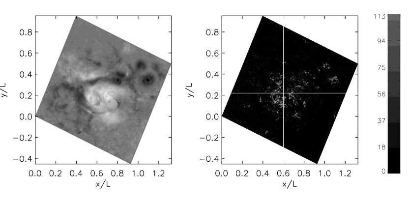
Figure 1: Left panel: The vertical magnetic field from the chromospheric magnetogram for AR 10486 at 18:46UT on 29 October 2003. Right panel: The estimate $\widetilde{f}_{h}(\alpha)/{\rm max}[B_{z}^{2}/(2\mu_{0})]$ of the magnitude of the horizontal Lorentz force for the same magnetogram. The horizontal and vertical lines correspond to $\widetilde{\langle x\rangle}(\alpha)/L$ and $\widetilde{\langle y\rangle}(\alpha)/L$ respectively.

4 Discussion

This paper addresses the problem of the origin dependence of virial theorem estimates of the magnetic energy of solar active regions. A method is presented for calculating an origin-independent energy based on estimation of terms missing from the usual statement of the virial theorem, involving integrals of moments of the Lorentz forces. The method assumes the forces are located close to the height where magnetic field measurements are taken. If measurements are available at two heights in the low atmosphere, the terms may be directly estimated using observed horizontal and vertical field gradients. If (as is generally the case) measurements are available corresponding to a single height, the terms may be estimated using observed horizontal field gradients together with vertical field gradients coprresponding to a linear force-free model of the field. This latter procedure is demonstrated in application to five vector magnetograms, including a chromospheric magnetogram, and the results are given in Table 1. The results suggest that, at least for photospheric magnetograms, the large uncertainties associated with field measurements and with the estimation of the force-free parameter makes obtaining a meaningful free energy estimate a difficult task.

The accuracy of the pseudo-Monte Carlo method of Metcalf, Leka & Mickey (2005) is also investigated. It is shown that this method provides a reliable estimate of magnetic energy provided Lorentz forces are approximately uniformly distributed over the plane where measurements originate. More generally, it is necessary to take account of the distribution of Lorentz forces, for example using the methods described here. The result of the pseudo Monte-Carlo procedure is shown to correspond to the simple virial theorem estimate with the origin at the center of the field of view. An analytic expression for the standard deviation associated with the averaging procedure is also given [Equation (A12)].

The use of vertical gradients from a linear force-free field to estimate Lorentz forces is a crude approach, since linear force-free fields have identically zero Lorentz forces. However, the point is that the horizontal gradients of the observed field contain important information about the Lorentz forces. Although the vertical gradients are inaccurate, the improved virial estimate contains the additional information in the horizontal gradients, and hence may provide a more accurate estimate of the total energy. The approach is similar to one already widely used in ambiguity resolution, in which observed horizontal field gradients together with the vertical gradients of a linear force-free field are used to estimate ${\rm div}\,{\bf B}$ (Metcalf 1994).

It should be noted that the method outlined here is more general than the specific approach using the linear force-free vertical gradients, and may be improved by using better estimates of the vertical gradients, if available. We note that the uncertainties $\sigma(\alpha)$ in the energy estimates associated with the linear force-free vertical gradients were found to be larger than the uncertainties $\sigma({\bf B})$ associated with the field measurements. This also suggests the need for improved estimates of the vertical field gradients. It is expected that the method will provide better estimates if magnetograms giving the field simultaneously at two heights are available (e.g. at the photospheric and chromospheric levels), and we are currently investigating this. Such a procedure will also allow a test of the use of the linear force-free model for the vertical gradients.

The nature of the non-zero Lorentz forces has not been described. In general there may be local pressure, gravity, and inertial forces present at the level of the measurements, which will lead to local non-zero values of $f_{x}$ and $f_{y}$. It should also be noted that there may be substantial non-zero net Lorentz forces due to flux closing outside the field of view of a magnetogram, even if the local Lorentz forces are themselves small. Generally magnetograms only have flux balanced to within 10% or so, since fields of view are relatively small, and active regions can have connections to surrounding flux (e.g. see the top row of Table 1), so this is an important consideration. This effect will also be present with chromospheric magnetograms. We note that the present method is able to model this kind of global departure from force-freeness.

With the advent of improved vector magnetographs, including instruments in space, it is important that as much information as possible is extracted from the data, and the present method may be useful in this regard. Hopefully this work goes some way towards countering the assertion of McClymont, Jiao & Mikic (1997) that “any virial theorem estimate of the free energy is meaningless”.

Appendix A Averaging $W_{0}$ over origins within the field of view

The pseudo-Monte Carlo method of Metcalf, Leka & Mickey (2005) involves averaging the simple virial estimate (1) over many choices of origin within the field of view. It is straightforward to calculate the resulting average and standard deviation based on a single evaluation of the virial integral together with $F_{x}$ and $F_{y}$, subject to the assumption that the measured field lies in a plane tangent to the photosphere. Denoting the virial estimate with the origin corresponding to the lower left hand corner of the magnetogram by $W_{0}$, then following Equation (2), the estimate with a choice of origin $(x_{0},y_{0})$ is $W_{0}^{\prime}=W_{0}+x_{0}F_{x}+y_{0}F_{y}$. We require the average of $W_{0}^{\prime}$ over choices of $x_{0}$ and $y_{0}$, which we denote

$$\overline{W_{0}^{\prime}}=W_{0}+\overline{x}_{0}F_{y}+\overline{y}_{0}F_{y},$$ (A1)

where

$$\overline{x}_{0}=\left.\int_{z=0}x_{0}dx_{0}dy_{0}\right/\int_{z=0}dx_{0}dy_{0},$$ (A2)

and similarly for $\overline{y}_{0}$.

The integrals for $\overline{x}_{0}$ and $\overline{y}_{0}$ may be evaluated by changing variables in the integration to image plane co-ordinates $\xi$ and $\eta$, aligned with terrestrial north and west respectively, and integrating over $0\leq\xi\leq L$, $0\leq\eta\leq L$. The image plane and heliographic co-ordinates are related by the linear transformation (e.g. Gary & Hagyard 1990)

$$\left(\begin{array}[]{c}\xi\\ \eta\end{array}\right)=\left(\begin{array}[]{cc}c_{11}&c_{12}\\ c_{21}&c_{22}\end{array}\right)\left(\begin{array}[]{c}x\\ y\end{array}\right),$$ (A3)

where

$$c_{11} = \cos P\cos\ell_{c}-\sin P\sin B_{0}\sin\ell_{c},$$

$$c_{12} = -\cos P\sin B_{c}\sin\ell_{c}-\sin P(\cos B_{0}\cos B_{c}+\sin B_{0}\sin B_{c}\cos\ell_{c}),$$

$$c_{21} = \sin P\cos\ell_{c}+\cos P\sin B_{0}\sin\ell_{c},$$

$$c_{22} = -\sin P\sin B_{c}\sin\ell_{c}+\cos P(\cos B_{0}\cos B_{c}+\sin B_{0}\sin B_{c}\cos\ell_{c}).$$ (A4)

In these expressions $B_{0}$ is the latitude of the disk center and $P$ is the angle between the projection of the rotation axis of the Sun on the sky and terrestrial north, measured eastward from north. The angle $\ell_{c}$ is the longitude of the center of the region of interest with respect to the meridian passing through disk center (the Central Meridional Distance, or CMD), and $B_{c}$ is the latitude of the center of the region of interest.

To perform the integrations it is also necessary to calculate the Jacobian of the transformation (A3), which is the reciprocal of the cosine of the angle $\Theta$ between the normal vector to the tangent plane and the line-of-sight to the observer. Specifically we require

$$\frac{\partial(x,y)}{\partial(\xi,\eta)} = \left|\begin{array}[]{cc}c_{11}&c_{12}\\ c_{21}&c_{22}\end{array}\right|^{-1}$$

$$= \left(\sin B_{0}\sin B_{c}+\cos B_{0}\cos B_{c}\cos\ell_{c}\right)^{-1}$$

$$= \sec\Theta.$$ (A8)

Using Equations (A3) and (A), the integrals for $\overline{x}_{0}$ and $\overline{y}_{0}$ evaluate to

$$\overline{x}_{0} = \sec\Theta\frac{L}{2}(c_{22}-c_{12}),$$

$$\overline{y}_{0} = \sec\Theta\frac{L}{2}(-c_{21}+c_{11}).$$ (A9)

From the inverse of the transformation (A3) it follows that $(\overline{x}_{0},\overline{y}_{0})$ corresponds to the center of the image plane field of view:

$$\overline{x}_{0} = x(\xi=L/2,\eta=L/2),$$

$$\overline{y}_{0} = y(\xi=L/2,\eta=L/2).$$ (A10)

Hence the estimate $\overline{W_{0}^{\prime}}$ corresponds to choosing the origin at the center of the field of view.

Following a similar procedure the standard deviation

$$\sigma_{0}=\left\{\overline{(W_{0}^{\prime}-\overline{W_{0}^{\prime}})^{2}}\right\}^{1/2}$$ (A11)

may be evaluated to give

$$\sigma_{0}=\sec\Theta\frac{L}{2\sqrt{3}}\left[(c_{22}^{2}+c_{12}^{2})F_{x}^{2}-2F_{x}F_{y}(c_{22}c_{21}+c_{12}c_{11})+(c_{21}^{2}+c_{11}^{2})F_{y}^{2}\right]^{1/2}.$$ (A12)

Finally, it should be noted that the computational procedure followed by Metcalf, Leka & Mickey (2005) takes into account the curvature of the Sun’s surface, which is neglected here. When curvature is included, the results of the pseudo-Monte Carlo procedure will be slightly different from the estimates given by Equations (A1), (A), and (A12).

Table 1: Results of applying the method to five vector magnetograms.

	AR 9077	AR 10306	AR 10386	AR 10397	AR 10486
$\phi$	-0.099	0.46	-0.14	0.37	-0.0013
$U$ [J]	$5.9\times 10^{25}$	$1.6\times 10^{26}$	$3.2\times 10^{25}$	$1.5\times 10^{26}$	$4.4\times 10^{26}$
$W_{0}$ [J]	$-1.5\times 10^{26}$	$5.5\times 10^{26}$	$-3.0\times 10^{26}$	$-3.1\times 10^{26}$	$7.7\times 10^{26}$
$\overline{W}_{0}$ [J]	$5.4\times 10^{25}$	$2.4\times 10^{26}$	$1.1\times 10^{26}$	$2.4\times 10^{26}$	$7.0\times 10^{26}$
$\overline{W}_{0}-U$ [J]	$-4.6\times 10^{24}$	$8.0\times 10^{25}$	$7.7\times 10^{25}$	$9.9\times 10^{25}$	$2.6\times 10^{26}$
$|F_{x}/F_{0}|$	0.0041	0.0060	0.093	0.13	0.0055
$|F_{y}/F_{0}|$	0.079	0.046	0.075	0.027	0.0041
$\alpha\pm\sigma_{\alpha}$ [$L^{-1}$]	$-2.8\pm 7.1$	$0.2\pm 8.9$	$15.1\pm 10.5$	$-0.4\pm 8.4$	$-8.3\pm 11.2$
$\widetilde{\langle x\rangle}(\alpha)/L$	0.54	0.084	0.38	0.64	0.60
$\widetilde{\langle y\rangle}(\alpha)/L$	0.44	0.70	0.53	0.14	0.22
$\widetilde{W}(\alpha)-U$ [J]	$-2.0\times 10^{25}$	$5.8\times 10^{25}$	$2.3\times 10^{25}$	$4.5\times 10^{26}$	$2.6\times 10^{26}$
$\sigma({\bf B})$ [J]	$4.2\times 10^{24}$	$5.5\times 10^{24}$	$1.1\times 10^{24}$	$9.0\times 10^{25}$	$1.1\times 10^{25}$
$\sigma(\alpha)$ [J]	$8.3\times 10^{24}$	$3.0\times 10^{25}$	$6.2\times 10^{25}$	$2.6\times 10^{26}$	$1.2\times 10^{25}$

References

- Alissandrakis (1981) Alissandrakis, C.E. 1981, Astron. Astrophys. 100, 197-200
- Aly (1984) Aly, J.J. 1984, ApJ 283, 349-362
- Aly (1989) Aly, J.J. 1989, Sol. Phys. 120, 19-48
- Chandrasekhar (1961) Chandrasekhar, S. 1961, Hydrodynamic and Hydromagnetic Stability (Oxford: Clarendon Press)
- Gary & Hagyard (1990) Gary, G.A., & Hagyard, M.J. 1990, Sol. Phys. 126, 21-36
- Gary, Moore, Hagyard & Haisch (1987) Gary, G.A., Moore, R.L., & Haisch, B.M. 1987, ApJ 314, 782-794
- Georgoulis & LaBonte (2004) Georgoulis, M.K., & LaBonte, B.J. 2004, ApJ 615, 1029-1041
- Keller, Harvey & Giampapa (2003) Keller, C.U., Harvey, J.W., & Giampapa, M.S. 2003, in Innovative Telescopes and Instrumentation for Solar Astrophysics, ed. S.L. Keil & S.V. Avakyan (Proc. SPIE, vol. 4853) 194-204
- Klimchuk, Canfield & Rhoads (1992) Klimchuk, J.A., Canfield, R.C., & Rhoads, J.E., ApJ 385, 327-343
- LaBonte, Mickey & Leka (1999) LaBonte, B.J., Mickey, D.L., & Leka, K.D. 1999, Sol. Phys. 189, 1-24
- Leka & Skumanich (1999) Leka, K.D., Skumanich, A. 1999, Sol. Phys. 188, 3-19
- Low (1982) Low, B.C. 1982, Sol. Phys. 77, 43-61
- McClymont, Jiao & Mikic (1997) McClymont, A.N., Jiao, L., and Mikic, Z. 1997, Sol. Phys. 174, 191-218
- Metcalf (1994) Metcalf, T.R. 1994, Sol. Phys. 155, 235-244
- Metcalf et al. (1995) Metcalf, T.R., Jiao, L., McClymont, A.N., Canfield, R.C., & Uitenbroek, H. 1995, ApJ 439, 474-481
- Metcalf, Leka & Mickey (2005) Metcalf, T.R., Leka, K.D., & Mickey, D.L. 2005, ApJ 623, L53-L56
- Molodenskii (1969) Molodenskii, M.M. 1969, Sov. Astron. AJ 12, 585
- Molodensky (1974) Molodensky, M.M. 1974, Sol. Phys. 39, 393-404
- Moon et al. (2002) Moon, Y.-J., Choe, G.S., Yun, H.S., Park, Y.D., & Mickey, D.L. 2002, ApJ 568, 422-431
- Sakurai (1987) Sakurai, T. 1987, Sol. Phys. 113, 137-142
- Venkatakrishnan & Gary (1989) Venkatakrishnan, P., & Gary, G.A. 1989, Sol. Phys. 120, 235-247
- Wheatland (2001) Wheatland, M.S. 2001, Publ. Astron. Soc. Aus. 18, 351-354