Galaxies at $z\sim 6$: The $UV$ Luminosity Function and Luminosity Density from 506 HUDF, HUDF-Ps, and GOODS $i$-dropouts

Abstract

We have detected 506 $i$-dropouts ($z\sim 6$ galaxies) in deep, wide-area HST ACS fields: HUDF, enhanced GOODS, and HUDF-Parallel ACS fields (HUDF-Ps). The contamination levels are $\lesssim 8$% (i.e., $\gtrsim 92$% are at $z\sim 6$). With these samples, we present the most comprehensive, quantitative analyses of $z\sim 6$ galaxies yet and provide optimal measures of the $UV$ luminosity function (LF) and luminosity density at $z\sim 6$, and their evolution to $z\sim 3$. We redetermine the size and color evolution from $z\sim 6$ to $z\sim 3$. Field-to-field variations (cosmic variance), completeness, flux, and contamination corrections are modelled systematically and quantitatively. After corrections, we derive a rest-frame continuum UV ($\sim 1350\AA$) LF at $z\sim 6$ that extends to $M_{1350,AB}$ $\sim-17.5$ ($0.04L_{z=3}^{*}$). There is strong evidence for evolution of the LF between $z\sim 6$ and $z\sim 3$, most likely through a brightening ($0.6\pm 0.2$ mag) of $M^{*}$ (at 99.7% confidence) though the degree depends upon the faint–end slope. As expected from hierarchical models, the most luminous galaxies are deficient at $z\sim 6$. Density evolution ($\phi^{*}$) is ruled out at $>$99.99% confidence. Despite large changes in the LF, the luminosity density at $z\sim 6$ is similar ($0.82\pm 0.21\times$) to that at $z\sim 3$. Changes in the mean UV color of galaxies from $z\sim 6$ to $z\sim 3$ suggest an evolution in dust content, indicating the true evolution is substantially larger: at $z\sim 6$ the star formation rate density is just $\sim 30$% of the $z\sim 3$ value. Our UV luminosity function is consistent with $z\sim 6$ galaxies providing the necessary UV flux to reionize the universe.

1. Introduction

The deep $z_{850}$-band capabilities of the Hubble Space Telescope (HST) Advanced Camera for Surveys (ACS) greatly enhanced the ability of astronomers to identify and observe galaxies at $z\sim 6$. Flux in the $z_{850}$-band can be contrasted with flux in the $i_{775}$-band, allowing for identification of $z\sim 6$ $i_{775}$-dropouts. Early studies revealed that $i$-dropouts were both smaller (Bouwens et al. 2003b; Stanway et al. 2004b; Bouwens et al. 2006b, hereafter, B06b) and less numerous than dropouts at lower redshifts (Stanway et al. 2003; Bouwens et al. 2003b; Dickinson et al. 2004; Stanway et al. 2004b; B06b). However, since much of the early work was at bright magnitudes ($z_{850,AB}\lesssim 27$), it was still quite unclear from these studies how this population extended to fainter magnitudes or lower surface brightnesses.

With the availability of significantly deeper $i$ and $z$ data from the Hubble Ultra Deep Field (HUDF; Beckwith et al. 2006) and the HUDF-Ps (Bouwens et al. 2004b), this situation is largely changed. There are already a number of papers that take advantage of this depth to comment on the faint-end slope (Bouwens et al. 2004a; Bunker et al. 2004, hereafter, BSEM04; Yan & Windhorst 2004b), the rest-frame UV colors (Stanway et al. 2005; Yan et al. 2005), and the surface brightness distribution at $z\sim 6$ (BSEM04; Bouwens et al. 2004b). These data have also provided us with some new insight into the long standing question of how the universe was reionized. Some authors (e.g., Yan & Windhorst 2004b; Lehnert & Bremer 2003) have argued that it is largely the faint galaxies that were instrumental in this process, while others have emphasized the role that possible evolution in metallicity or the initial mass function (IMF) may have on the process (Stiavelli et al. 2004b). Finally, other groups (e.g., BSEM04) have even questioned whether the observed galaxy population is sufficient to reionize the universe at all.

While providing many interesting initial results, there were a number of limitations to these early analyses. Some (e.g., BSEM04) restricted themselves to a bright limit (in their analyses of the two most notable data sets) to minimize the importance of incompleteness, flux, or contamination corrections. Other analyses did not calculate the selection volume for their survey self-consistentally from the observed UV colors (but rather assumed a simple $z=5.5-6.5$ top-hat selection window: e.g., Yan & Windhorst 2004b). Moreover, none of these early studies made a detailed account of the uncertainties in their LF determinations or made an attempt to correct for field-to-field variations, which can be substantial ($\sim 35$% rms) for single 11.3 arcmin² ACS Wide-Field Camera (WFC) fields (Somerville et al. 2004; Bouwens et al. 2004a; BSEM04). Correcting for these variations is important for ensuring that a consistent normalization is used at bright, intermediate, and faint magnitudes and thus the derived luminosity function (LF) is not compromised. Particularly important in this regard are the implications for the faint-end slope and the number of lower luminosity galaxies. Such objects have the potential to provide the necessary UV flux to reionize the universe (Lehnert & Bremer 2003; Yan & Windhorst 2004b).

The purpose of this paper is to redress many of these limitations and provide a systematic analysis of $i$-dropouts from some of the deepest, widest area surveys available for study. We consider fields at three different depths. The two wide-area GOODS fields ($\sim$160 arcmin² each), here enhanced to include the extensive supernova search data, form the backbone of our probe, providing important statistics at the bright end while controlling for field-to-field variations. At the faint end, there is the Hubble Ultra Deep Field (HUDF; 11 arcmin²), which in addition to constraining the faint-end slope allows us to quantify the incompleteness, flux biases, and contamination in our shallower probes. Finally, at intermediate magnitudes, we have the two HUDF-Ps (17 arcmin² in total), which provide an important bridge between our faintest and brightest fields. Together these three data sets provide a good measure of the $i$-dropout surface density over a 5 mag baseline, from $z_{850,AB}\sim 24.5$ to 29.5.

This paper is structured as follows. We begin with a description of the data (§2), describe our selection criteria (§3), and then compile an $i$-dropout sample in the HUDF. We use the color information to make inferences about the contamination rate, intrinsic colors, and overall redshift distribution. We then proceed to an analysis of our shallower fields and incorporate the data from those fields into our $i$-dropout probe, deriving the $i$-dropout surface density from $z_{850,AB}\sim 24.5$ to 29.5. In §4, we compare the present probe with previous catalogs and surface density determinations. In §5, we use this surface density to derive a LF in the rest-frame UV ($\sim 1350\AA$) and compare it with the LF derived at $z\sim 3$ (Steidel et al. 1999). Finally, we discuss these results, comment on the likely physical implications (§6), and conclude (§7). We make use of appendices to develop some key technical issues, while not interrupting the flow of the paper. Where necessary, we use the “concordance cosmology” $(\Omega_{M},\Omega_{\Lambda},h)=(0.3,0.7,0.7)$. We note that the results are not very dependent on the details of the cosmology and that $M^{*}$ and $\phi^{*}$ change by $\lesssim 12$% (§5) when expressed in terms of the one year WMAP measurements $(\Omega_{M},\Omega_{\Lambda},h)=(0.24,0.76,0.73$; Spergel et al. 2003).

2. Observations

As noted above, the present analysis leverages data sets of three different depths to obtain a fairly optimal measure of the number densities of $i$-dropouts over a 5 mag baseline. Table 1 provides a summary of these data sets.

Table 1Observational Data.

	Detection Limits	PSF FWHM	Areal Coverage
Passband	(10$\sigma$)	(arcsec)	(arcmin2)
HUDF
$B_{435}$	29.6	0.09	11.2
$V_{606}$	30.0	0.09	11.2
$i_{775}$	29.9	0.09	11.2
$z_{850}$	29.2	0.10	11.2
$J_{110}$	26.9	0.33	5.8
$H_{160}$	26.7	0.37	5.8
HUDF-Ps
$B_{435}$	28.9	0.09	17.0
$V_{606}$	29.2	0.09	17.0
$i_{775}$	28.8	0.09	17.0
$z_{850}$	28.5	0.10	17.0
GOODS fields
$B_{435}$	28.2	0.09	316
$V_{606}$	28.4	0.09	316
$i_{775}$	27.7	0.09	316
$z_{850}$	27.5	0.10	316
$J$	$\sim 25$	$\sim$0.45′′	131
$K_{s}$	$\sim 24.5$	$\sim$0.45′′	131

2.1. ACS HUDF

The $B_{435}V_{606}i_{775}z_{850}$ images used for this analysis are the v1.0 reductions of the HUDF (Beckwith et al. 2006), binned on a 0.03^′′ pixel scale. While the observations cover $\sim$12 arcmin², our search area was restricted to the deepest 11.2 arcmin². The zeropoints used for these images are the latest values from the continuing ACS calibrations (Sirianni et al. 2005). Photometry performed using these zeropoints was offset slightly to account for the estimated Galactic absorption $E(B-V)=0.007$ (Schlegel, Finkbeiner, & Davis 1998). The $10\sigma$ limits for these images were 29.6, 30.0, 29.9, and 29.2, respectively, in 0.2^′′-diameter aperture. Point-spread functions (PSFs) were 0.09-0.10^′′ FWHM.

Extremely deep Near-Infrared Camera and Multi-Object Spectrometry (NICMOS) coverage is available over a portion of the HUDF (5.76 arcmin²; Thompson et al. 2005). That program included eight orbits in the NIC3 $J_{110}$ filter and eight orbits in the NIC3 $H_{160}$ filter over nine separate pointings, for a total of 144 orbits. The pointings were arranged in a $3\times 3$ grid, each separated by 45^′′. Although there is some variation in depth across the mosaic, typical $5\sigma$ limits for the images were 27.6 and 27.4 in the $J_{110}$ and $H_{160}$ passbands (0.6^′′-diameter aperture), respectively. Our reduction of the NICMOS data was a slight improvement on that initially made available with the treasury release and was made possible by more exact position matching with the HUDF $z_{850}$-band image. This reduction is described in more detail in Thompson et al. (2005). The resulting NIC3 PSFs had FWHMs of 0.33^′′ and 0.37^′′  in the $J_{110}$ and $H_{160}$ bands, respectively. The $F110W$ and $F160W$ zero points used are those recently determined by STScI (de Jong et al. 2006; see also Coe et al. 2006). These zeropoints are offset by $-0.16$ and $-0.04$ (de Jong et al. 2006) from those previously made available by the Space Telescope Science Institute (STScI; 2004 June).

2.2. HUDF ACS Parallels

The two HUDF-Ps were taken in parallel to the HUDF NICMOS observations (GO-9803: Thompson et al. 2005). Each field consists of 72 orbits of ACS observations (9 orbits of $B_{435}$, 9 orbits of $V_{606}$, 18 orbits of $i_{775}$, 27 orbits of $z_{850}$, and 9 orbits of G800L) that reaches nearly $\sim 1$ mag deeper than the original 5-epoch ACS GOODS observations. They also reach fainter ($\sim 0.2-0.4$ mag) than the WFPC2 HDF-N (Williams et al. 1996) and HDF-S (Williams et al. 2000). Processing of the data included alignment, background subtraction, cosmic ray rejection, and drizzling onto a 0.03^′′  grid, and was performed by the “Apsis” pipeline (Blakeslee et al. 2003). Artifacts in the original exposures such as satellite trails or the “figure eight” patterns (resulting from scattered light off the internal dewars) were explicitly masked out before drizzling the images together. The reductions of these fields used in this paper are different from those described in several previous publications (Blakeslee et al. 2004; Bouwens et al. 2004a). Our principal reason for this was to bin the data on a very similar 0.03^′′-pixel scale to that available for the ACS GOODS fields (§2.3) and the HUDF (Beckwith et al. 2006). The similar pixel scale made it straightforward to degrade the deeper data to the quality of the shallower data and therefore estimate quantities like the completeness, flux biases, and contamination rate (see Appendix C).

To maximize depth, we combined the ACS parallel data (Thompson et al. 2005) with overlapping ACS WFC exposures from the CDF-S GOODS (Giavalisco et al. 2004a), GEMS (Rix et al. 2004), and SNe search programs (A. Riess et al. 2006, in preparation). Incorporating the latter data resulted in modest increases in the mean depth of our images ($+0.2$ mag). Only regions having exposure times in excess of 5 orbits, 11 orbits, and 18 orbits in the $V_{606}$, $i_{775}$, and $z_{850}$ bands, respectively, are considered in our selection (or equivalently their $10\sigma$ depths were required to exceed 28.9, 28.6, and 28.1 in the $V_{606}$, $i_{775}$, and $z_{850}$ bands, respectively, in a 0.2^′′-diameter apertures). This corresponded to 10.0 arcmin² in the first HUDF-Parallel [hereafter, referred to as HUDFP1] and 7.0 arcmin² in the second [hereafter, referred to as HUDFP2]. The $10\sigma$ depths for the deepest portion of these parallels were 28.9, 29.2, 28.8, and 28.5 in the $B_{435}$, $V_{606}$, $i_{775}$, and $z_{850}$ bands, respectively, in 0.2^′′-diameter apertures ($\sim$0.7-1.1 mags less deep than the HUDF).

2.3. ACS GOODS

The current analysis makes use of our own reductions of the ACS data available over the two GOODS fields ($\sim 160$ arcmin²). Though a public reduction of the data over this area was available (i.e., the GOODS version 1.0 reduction: Giavalisco et al. 2004a), it did not include the significant amounts of ACS data taken over these fields after the initial 398-orbit GOODS campaign. These include 195 orbits of $V_{606}i_{775}z_{850}$ data taken for additional SNe searches (A. Riess et al. 2006, in preparation; S. Perlmutter et al. 2006, in preparation), $\gtrsim 100$ orbits of $z_{850}$-band data for SNe follow-up (A. Riess et al. 2006, in preparation; S. Perlmutter et al. 2005, in preparation), $\sim 40$ orbits of overlapping $V_{606}$ and $z_{850}$ data from the GEMS program (Rix et al. 2004), and 128 orbits of $B_{435}V_{606}i_{775}z_{850}$ data over the ACS parallels to the HUDF NICMOS field (Thompson et al. 2005). These data substantially enhance the GOODS version 1.0 data set, and should largely be included in the GOODS version 2.0 release. Instead of waiting for the release, we carried out our own reduction. Similar to our handling of the HUDF-Parallel ACS fields, we processed the ACS data with our “Apsis” pipeline (Blakeslee et al. 2003). They were drizzled onto the same astrometric grid as the images (35 individual 8k x 8k frames) which made up the v1.0 reductions of the two GOODS fields (Giavalisco et al. 2004a). These images–and our own reductions–were done on a 0.03^′′ pixel scale very similar to the HUDF. The approximate $10\sigma$ depths of those data were 28.2, 28.4, 27.7, and 27.5 in the $B_{435}$, $V_{606}$, $i_{775}$, and $z_{850}$ bands, respectively. These data reach nearly $\sim 0.15$ mag and $\sim 0.4$ mag deeper in the $i_{775}$ and $z_{850}$ bands, respectively, than the GOODS v1.0 reductions.

One complication with the analysis of the two GOODS fields is the notable variation in the depth. The extensive overlap regions between adjacent exposures in the ACS tiling ($\sim 7$ arcmin² for each field) are appreciably deeper ($\sim 0.4$ mag), the many outer regions ($\sim 30$ arcmin² for each field) only covered by three epochs of data (5 epochs including the SNe search data) are shallower ($\sim 0.3$ mag), and other regions of these fields with missing exposures (e.g., due to guide star acquisition problems) also are shallower (Giavalisco et al. 2004a). As we demonstrated in an earlier study on the $i$-dropouts in the RDCS1252-2927 field (Bouwens et al. 2003b), such variations can have a dramatic impact on the number of $i$-dropouts selected (changing the numbers by factors of $\sim 1.8$ for just $\sim$0.4 mag alterations in depth), and therefore any selection of $i$-dropouts off the undegraded GOODS images requires an accurate accounting for these variations. This could be done, for example, by laying down objects at random positions across the GOODS mosaic and then attempting to recover them. Instead of adopting this more involved approach, we took a simpler route, degrading the entire frame to a uniform S/N and ignoring regions below this S/N in the object selection. Our procedure for executing the degradation is detailed in Appendix B. The threshold we settled on was $0.1$ mag brighter than that obtained with a 2.5, 3.5, and 9-orbit exposure in the $V_{606}$, $i_{775}$, and $z_{850}$ bands, respectively, and was chosen as a compromise between depth and area. This threshold is equivalent to 10$\sigma$ depths of 28.3, 27.5, and 27.4 in the $V_{606}$, $i_{775}$, and $z_{850}$ bands, respectively. Throughout this work, this is what we mean when we refer to the S/N levels of the GOODS fields (or to deeper fields degraded to GOODS depth).

We also made use of the Infrared Spectrometer and Array Camera (ISAAC) $JK_{s}$ data for the CDF-S GOODS field (B. Vandame et al. 2006, in preparation) to better estimate the contamination from lower redshift interlopers. The data consist of 21 separate $\sim$3-4 hr $2.5^{\prime}\times 2.5^{\prime}$ ISAAC exposures in the $J$ ($\sim 1.25\mu m$) and $K_{s}$ ($\sim 2.16\mu m$) bands that reach $\sim$25.7 and $\sim$25 AB magnitudes ($5\sigma$), respectively, in a 0.8^′′-diameter aperture. The entire mosaic covers 131 arcmin² or about $\sim 85$% of the ACS GOODS area. B. Vandame et al. (2006, in preparation) estimated the seeing for the frames to range from 0.31^′′ to 0.66^′′, with a median value of 0.46^′′. Zero points for the individual ISAAC frames were derived by matching photometry of $\sim$50 stars on each frame with the shallower SOFI (Arnouts et al. 2001) and Two Micron All Sky Survey (2MASS; Skrutskie et al. 1997) images.

As a check on the zero points, we performed photometry on the $\sim 20$ $z\sim 0.4-1.0$ E/S0s in each ISAAC frame (ACS $BViz$ + ISAAC $JK_{s}$ bands) and then fit a spectral energy distribution (SED) to the six optical-infrared fluxes. While our $K_{s}$-band fluxes are in excellent agreement with the fit results, we noticed that our $J$-band fluxes were generally $\sim 0.1$ mag fainter than expected. Since B. Vandame et al. (2006, in preparation) noted a similar $\sim 0.1$ mag faintward offset relative to the photometry of the K20 survey (Cimatti et al. 2002), we took this offset to be real and offset the $J$-band zeropoints quoted by B. Vandame et al. (2006, in preparation) by 0.1 mag. No such shifts were applied to the $K_{s}$-band fluxes. Similarly, the seeing estimates obtained for different ISAAC images (B. Vandame et al. 2006, in preparation) were examined and compared with our own estimates. In general, the FWHMs we obtained were $\sim 0.02$^′′  to $\sim 0.05$^′′  larger than the B. Vandame et al. (2006, in preparation) estimates. We elected to apply our estimates throughout in determining the optical-infrared colors of objects in the CDF-South GOODS field (i.e., Appendix D4.1). Given that our only use of $J$ and $K_{s}$ photometry in this study is for quantifying contamination, these adjustments should have no large effect on the other quantities derived here.

3. Analysis

Our procedure for doing object detection and photometry is identical to that detailed in a number of previous publications by our group (e.g., Bouwens et al. 2003a; Bouwens et al. 2006a, hereinafter, B06a). SExtractor (Bertin & Arnouts 1996) was run in double-image mode, with the $z_{850}$-band images used for object detection and the other images used as the measurement images. The infrared coverage–although superior in probing beyond the break–was not used in the detection procedure because (1) the signal-to-noise ratio (S/N) and resolution of these images were in general much poorer than the $z_{850}$-band images and (2) these images–where available–tended to be very inhomogeneous in nature. Photometry was done using two scaled Kron (1980) apertures, the smaller ones to measure colors and the larger ones to convert these colors to total magnitudes. Small corrections were applied to the total magnitudes ($0.1$ mag to the $B_{435}$, $V_{606}$, and $i_{775}$ bands and $0.125$ mag in the $z_{850}$ band: Sirianni et al. 2005) to account for the flux that falls outside these apertures (typically $\sim 0.8^{\prime\prime}$ in diameter). Optical-infrared colors were obtained by degrading the optical images to the same PSF as the coincident infrared image and then measuring the flux in an aperture that maximized the S/N (typically 0.8^′′-1.4^′′-diameter apertures).

One minor issue in the construction of our $i$-dropout catalogs was the choice of the SExtractor deblending parameter. A small value for this parameter minimizes blending with foreground sources, but also causes many of the more clumpy $i$-dropouts to split into multiple pieces. Conversely, a large value for this parameter largely avoids such splitting, but results in more blending with foreground sources. After extensive testing, we opted to use a larger value for the deblending parameter (i.e., DEBLEND_MINCONT = 0.15) than the defaults (i.e., DEBLEND_MINCONT = 0.005). Although this results in a greater degree of blending (e.g., 17% of $i$-dropouts are blended with foreground objects in the HUDF vs. 11% using much smaller deblending parameters: Appendix D1), it should avoid splitting physically-associated systems into multiple pieces–which would result in small systematic errors. Corrections can be made for these additional incompleteness levels (see Appendix D1). To ensure that the object blending was reasonable, a detailed visual inspection was performed on each of the objects in our samples (§3.2; §3.4). No objects were found that included any obvious contribution from foreground sources. The highly unique colors of dropout sources made this check a fairly unambiguous process.

3.1. $i$-dropout Selection

As in several previous publications on this subject (Stanway et al. 2003; Bouwens et al. 2004a; Dickinson et al. 2004; B06a), $i$-dropouts are selected using a simple $(i_{775}-z_{850})_{AB}$ cut. At intermediate magnitudes ($24<z_{850,AB}<27$), such cuts have already been shown to be quite efficient at isolating objects with blue $z-J$ colors indicative of $z\sim 6$ starbursts (Stanway et al. 2003; Bouwens et al. 2003b; Dickinson et al. 2004; Stanway et al. 2005; B06a). Our choice of a more inclusive $(i_{775}-z_{850})_{AB}>1.3$ criterion rather than the $>1.4$ and $>1.5$ criteria used in previous work (Bouwens et al. 2003; Bouwens et al. 2004a; B06a) was motivated by our desire to maximize the size of our sample. While this also results in a somewhat higher contamination rate (Appendix D4), an increasing amount of data is now available, both in the IR (Thompson et al. 2005; Vandame et al. 2006, in preparation) and with the ACS GRISM (Pirzkal et al. 2004; Malhotra et al. 2005) to better constrain the contamination. Note that in computing the $i-z$ color for selection, we set the $i$-band flux to its $2\sigma$ upper limit in the case of a non detection. In addition to our $i-z>1.3$ criteria, we also required that objects have $(V_{606}-z_{850})_{AB}$ colors redder than 2.8 or be non-detections ($<2\sigma$) in the $V_{606}$-band to exclude lower-redshift interlopers. Appendix A provides a justification for the $(V_{606}-z_{850})_{AB}$ color cut by comparing it with a number of intrinsically red galaxies uncovered in the CDF-South (Table 2). To guard against spurious sources that come in the form of low-surface brightness variations in the background (Appendix D4.4), we required that objects in the HUDF be at least $3.5\sigma$ detections in a 0.3$\arcsec$-diameter aperture. The detection requirement was increased to 4 and 4.5 $\sigma$ for the HUDF-Ps and GOODS fields, respectively, to cope with the likely larger non-Gaussian signatures present in the smaller exposure stacks that comprise these data. Point sources brighter than some fiducial $z_{850}$-band magnitude (26.8 for GOODS fields, 27.5 for the HUDF-Ps, and 28.4 for the HUDF) were removed at this stage (point sources were defined to have SExtractor stellarity parameters $>0.75$). Faintward of these fiducial limits, point sources could no longer be reliably identified (their contribution was treated as a contamination fraction and estimated statistically: see Appendix D4.3). Table 3 contains a list of all objects excluded as stars. Finally, we carefully inspected all of our candidate $i$-dropouts to ensure that they did not arise from diffraction spikes around stars or the extended low-surface brightness wings around ellipticals.

Table 2A sample of intrinsically red $(i_{775}-z_{850})_{AB}>1,(z_{850}-J)_{AB}>0.8$, likely low-redshift objects identified in the CDF-S GOODS field that may serve as interlopers for our $i$-dropout samples (Figure A1, Figure D3).

							$r_{hl}$
R.A.	Decl.	$z$	$i-z$	$V-z$	$z-J$	$z-K_{s}$	(arcsec)
03:32:35.63	-27:43:10.1	21.97$\pm$0.01	1.1	2.7	1.0	1.7	0.30
03:32:39.41	-27:54:11.8	22.17$\pm$0.01	1.3	2.8	1.1	2.2	0.58
03:32:25.07	-27:52:49.3	22.28$\pm$0.01	1.1	2.7	0.9	1.9	0.33
03:32:17.15	-27:52:32.0	22.46$\pm$0.01	1.0	2.6	0.9	1.8	0.28
03:32:25.76	-27:43:47.3	22.49$\pm$0.02	1.1	2.4	1.1	2.2	0.60
03:32:43.93	-27:42:32.4	22.72$\pm$0.01	1.2	3.2	1.6	2.4	0.35

Table 3$i-z>1.3$ pointlike (stellar) sources not included in our $i$-dropout compilation.

								$r_{hl}$
Object ID	R.A.	Decl.	$z_{850}$	$i-z$	$z-J$	$z-K_{s}$	S/G	(arcsec)
HDFN-6581218516	12:36:58.12	62:18:51.6	23.02$\pm$0.01	1.5	—	—	0.93	0.09
CDFS-2295952287	03:32:29.59	-27:52:28.7	23.05$\pm$0.01	1.4	1.0	0.9	0.98	0.08
HDFN-7340515534	12:37:34.05	62:15:53.4	23.17$\pm$0.01	1.5	—	—	0.94	0.09
CDFS-2192345455	03:32:19.23	-27:45:45.5	23.30$\pm$0.01	1.3	0.8	1.0	0.96	0.08
CDFS-2181947466	03:32:18.19	-27:47:46.6	23.60$\pm$0.01	1.4	1.1	1.3	0.99	0.08
HDFN-6388514511	12:36:38.85	62:14:51.1	23.89$\pm$0.01	1.7	—	—	0.92	0.09

3.2. $i$-dropouts in the HUDF

Applying the above selection criteria to the HUDF results in a sample of 122 $i$-dropouts. Objects range in magnitude from $z_{850,AB}=25.0$ to 29.4 (the $8\sigma$ limit). At $z\sim 6$, this corresponds to $0.04-2.2$ times the characteristic rest-frame UV luminosity at $z\sim 3$ (Steidel et al. 1999). Table 4 summarizes the positions, magnitudes, $i-z$ colors, sizes, stellarities, $z-J_{110}$ colors, and $J_{110}-H_{160}$ colors of different objects in our HUDF $i$-dropout sample. $V_{606}i_{775}z_{850}$ color cutouts are provided in Figure 1 for the brightest 28 $i$-dropouts from the HUDF.

The deeper optical and infrared imaging available in the central region of the HUDF allow us to extend our knowledge of the contamination rate from low-redshift interlopers (e.g., dusty/evolved $z\sim 1-3$ objects) to fainter magnitudes ($z_{850,AB}\gtrsim 27$) than has been previously possible. While there have already been several studies using these data to argue that this contamination is small (Yan & Windhorst 2004b; Stanway et al. 2005), the present selection pushes slightly deeper. As in our analysis of the $i$-dropouts in RDCS1252-2927 and the CDF-S GOODS field (Bouwens et al. 2003b; B06a), we consider the canonical $(i_{775}-z_{850})$ versus $(z_{850}-J_{110})$ color-color plot (Figure 2). It is immediately apparent that the contamination rate from low-redshift interlopers is low. Only two of the 43 $i$-dropouts observed to $z_{850,AB}\sim 28.7$ had $z-J_{110}$ colors inconsistent with the expected position of $z\sim 6$ starbursts in color-color space (shaded orange region), suggesting a very low ($\sim$5%) contamination rate for the sample as a whole. Splitting the sample across several magnitude bins, we can obtain a magnitude-dependent contamination fraction (Table D7).

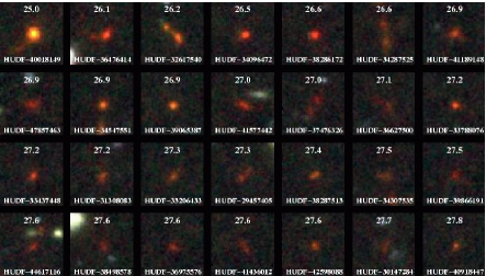
Figure 1.— Postage stamps ($V_{606}i_{775}z_{850}$ color images) of the brightest 24 $i_{775}$-dropouts from the HUDF. Objects are ordered in terms of their $z_{850}$-band magnitude. The $z_{850}$-band magnitudes and object IDs are shown above and below each object, respectively. Each postage stamp is 3.0^′′ in size. These high S/N images show definitive evidence for assymetries, mergers, and other interactions–similar to that seen at lower redshifts ($z\sim 2-5$).

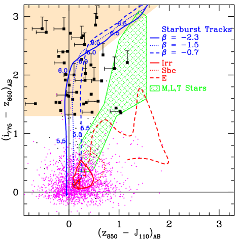
Figure 2.— The $i_{775}-z_{850}$/$z_{850}-J_{110}$ color-color diagram showing the photometry of objects (squares) in the HUDF NICMOS footprint. Objects undetected ($<2\sigma$) in the $V_{606}$ band or whose $(V_{606}-z_{850})_{AB}$ colors are redder than 2.8 (see Appendix A) are shown as filled black squares. Other objects in the photometric sample are displayed as magenta dots. The tracks made by starbursts of various UV spectral slopes $\beta$ are plotted here as a function of redshift to indicate the position of likely high-redshift $i$-dropouts (blue lines). For contrast, similar tracks have been included for a number of low-redshift templates to show the position of possible contaminants (red lines) along with the colors for early stellar types M0-T7 (Knapp et al. 2004; Geballe et al. 2002; Leggett al. 2002) (green hatched region). Although a $(i_{775}-z_{850})_{AB}>1.3$ criterion is used to select the $i$-dropout sample, almost all $i-z>1.3$ objects have very blue $(z_{850}-J_{110})_{AB}$ colors, as expected for bona-fide $5.5<z<7$ star-forming objects. (The shaded orange region shows the expected position of high-redshift objects and is used to estimate the contamination rate; see §3.2.) This suggests that our optically selected sample has a very low contamination rate ($\lesssim 5$%).

Table 4HUDF $i$-dropout sample.

								$r_{hl}$
Object ID	R.A.	Decl.	$z_{850}$	$i-z$	$z-J$	$J-H$	S/G	(arcsec)
HUDF-40018149	03:32:40.01	-27:48:14.9	24.99$\pm$0.01	1.6	0.0	$-$0.1	0.03	0.16
HUDF-36476414	03:32:36.47	-27:46:41.4	26.08$\pm$0.02	2.4	$-$0.1	0.4	0.03	0.19
HUDF-32617540	03:32:32.61	-27:47:54.0	26.21$\pm$0.03	1.4	—	—	0.03	0.24
HUDF-34096472	03:32:34.09	-27:46:47.2	26.50$\pm$0.02	2.2	—	—	0.06	0.12
HUDF-38286172	03:32:38.28	-27:46:17.2	26.56$\pm$0.03	2.7	0.0	0.0	0.06	0.12
HUDF-34287525	03:32:34.28	-27:47:52.5	26.58$\pm$0.05	1.5	0.3	$-$0.2	0.00	0.31

3.3. Rest-frame UV Colors and Redshifts

The $izJH$ photometry available for the HUDF can also be used to estimate both the rest-frame UV colors and redshifts for sample objects. The $z-J$/$J-H$ color-color diagram, in particular, serves as a useful starting point because at $z\gtrsim 5.9$ it provides a fairly unique mapping onto redshift and rest-frame UV color (Figure 3). Here we only include $i$-dropouts to a limiting magnitude of $H_{160,AB}\sim 27.7$. Faintward of this, there are substantial errors on the $J$ and $H$ photometry for individual objects, and hence it is only possible to estimate the average colors for this population. We obtain these colors by stacking the $i$-dropouts in two different faint magnitude intervals $27.4<z_{850,AB}<27.9$ and $27.9<z_{850,AB}<28.9$. Despite concerns about possible errors in the NICMOS zero points (§2.1), the position of the data is such as to suggest moderately blue rest-frame UV colors, i.e., $\beta=-2.0$, and a mean redshift somewhat below 6.

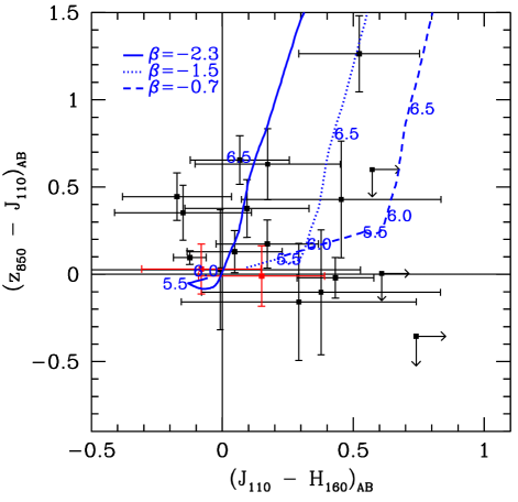
Figure 3.— The $(z_{850}-J_{110})$/$(J_{110}-H_{160})$ color-color diagram showing the photometry of all 14 bright $H_{160,AB}<27.7$ objects from the HUDF with deep NICMOS coverage. Each of these objects was required to be at least a $2\sigma$ detection in the $H_{160,AB}$ band. To make these measurements on even fainter dropouts, we included stacked photometry for objects in the magnitude bins $27.4<z_{850,AB}<27.9$ and $27.9<z_{850,AB}<28.9$ (red squares; §3.3). Model tracks are as in Figure 2. Errors are $1\sigma$ while the limits are $2\sigma$. The bright objects shown here are all clearly resolved and therefore non-stellar. The large fraction of objects with $J_{110}-H_{160}$ colors of $<0.3$ suggests a reasonably blue $\beta\sim-2.0$ population. Although a majority of the objects have $z_{850}-J_{110}$ colors suggestive of a pile-up at the lower redshift end of the window, i.e., $z\lesssim 6$, a few objects have $z_{850}-J_{110}$ colors consistent with being at higher redshift, i.e., $z\gtrsim 6.1$ (see also Malhotra et al. 2005).

Although illustrative, Figure 3 does not provide us with a very useful way of quantifying the mean properties of our sample, such as the redshift and rest-frame UV slope. To accomplish this, a better approach is to consider the distribution of $(z_{850}-J_{110})_{AB}$ and $(J_{110}-H_{160})_{AB}$ colors. This is analogous to the modeling we did in our previous work on $U$, $B$, and $V$-dropout samples from the Hubble Deep Field (HDF) and GOODS fields (B06a). The $(z_{850}-J_{110})_{AB}$ colors (reddened by the Ly$\alpha$ forest) are most useful for inferences about the mean redshift of the sample while the $(J_{110}-H_{160})_{AB}$ colors (redward of the break) are most useful for inferences about the mean rest-frame UV color of the sample. A schematic illustration of this is provided in the top panels of Figure 4, where the predicted $(z_{850}-J_{110})_{AB}$ and $(J_{110}-H_{160})_{AB}$ colors are shown as a function of the UV continuum slope $\beta$ (annotated) and redshift (right vertical axis). Using the blue lines as a guide, the $(z_{850}-J_{110})_{AB}$ colors of $i$-dropouts observed in the HUDF (shaded histogram: selected to have $H_{160,AB}\lesssim 27.7$) suggest that these objects are predominantly at $z\sim 5.5-6$. The $(J_{110}-H_{160})_{AB}$ colors indicate a mean $UV$ continuum slope $\beta$ of $\sim-2.0$.

We can make these inferences more rigorous by performing some simulations. To make the simulations as realistic as possible, we project a HUDF $B_{435}$-dropout sample (Bouwens et al. 2004b) to $z\sim 5-7$ and scale the sizes of individual $B$-dropouts as $(1+z)^{-1.1}$ (for fixed luminosity). This scaling is derived in §3.7 using the current data sets and is in good agreement with previous measurements (Bouwens et al. 2004a,b; B06b; Ferguson et al. 2004). The actual simulations are executed using our well-tested cloning software (Bouwens et al. 1998a,b; Bouwens et al. 2003a,b; B06b), which handles the artificial redshifting and reselection of individual objects. $B$-dropouts are distributed in redshift (assuming no clustering) according to the product of their individual $1/V_{max}$ and the available cosmological volume. Here, three mean rest-frame UV slopes are assumed for the simulations: $\beta=-2.2$, $-1.8$, and $-1.4$. A $1\sigma$ scatter of 0.5 (in the UV slope $\beta$) is assumed for each. The results of the simulations are shown in the bottom panels of Figure 4 (black lines) and compared with the observations. It seems clear that the observed $(J_{110}-H_{160})_{AB}$ colors (histogram) can be best fit by a model with a mean $\beta$ of $-2.0$, somewhere in between the $\beta=-2.2$ and $\beta=-1.8$ model results (dotted line). All models however yield a tail toward red $(z_{850}-J_{110})_{AB}$ colors that does not occur in the observations (histogram). This suggests a deficit of $i$-dropouts at the higher redshift end of the $z\sim 5.5-7$ selection window. To model this, we assumed that the space density of $i$-dropouts in the HUDF was a strong function of redshift, i.e., $e^{-(z-5.5)}$, while adopting the best-fitting mean-frame UV slope $\beta$ found above ($-2.0$). The results are shown in Figure 4 as a solid purple line and provide a rough fit to the median colors. We note that very similar conclusions have come from the GRAPES program (Malhotra et al. 2005), where even better redshift measurements are possible from the GRISM data. Malhotra et al. (2005) demonstrated that the majority of bright ($z_{850,AB}\lesssim 28$) $i$-dropouts in the HUDF (15 out of 23 objects) are at $z\sim 5.9\pm 0.2$.

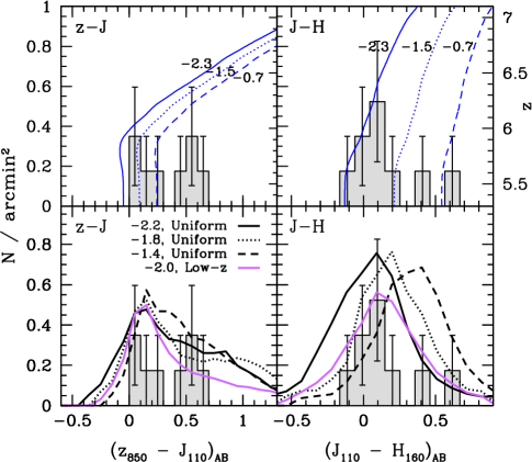
Figure 4.— Top panels; The observed $(z_{850}-J_{110})_{AB}$ and $(J_{110}-H_{160})_{AB}$ color distributions (histogram with $1\sigma$ Poisson errors). Overplotted is the color as a function of redshift (right-hand axis) for a range of $\beta^{\prime}s$: $\beta=-0.7$ (dashed blue line), $\beta=-1.5$ (dotted blue line), and $\beta=-2.3$ (solid blue line). The binned colors were derived from $i$-dropouts in the HUDF with $H_{160,AB}\lesssim 27.8$. Bottom panels; The observed $(z_{850}-J_{110})_{AB}$ and $(J_{110}-H_{160})_{AB}$ color distributions (histogram) vs. that recovered from simulations assuming three different mean rest-frame UV slopes $\beta=-2.2$ (solid black line), $\beta=-1.8$ (dotted black line), and $\beta=-1.4$ (dashed black line). To model the deficit of objects with large $(z_{850}-J_{110})$ colors, we also included the results from a simulation in which the object density was proportional to $e^{-(z-5.5)}$ (assuming a mean $\beta$ of $-2.0$). Together the $z-J_{110}$ (providing information on Ly$\alpha$ forest attenuation) and $J_{110}-H_{160}$ (constraining the spectral slope) colors place good constraints on the rest-frame UV slope $\beta$ and redshift. These results suggest that most $i$-dropouts in the HUDF NICMOS footprint lie below $z\sim 6.2$ with a mean $\beta$ of $-2.0$. More details can be found in §3.3.

3.4. $i$-dropouts in the GOODS/HUDF-P fields

To control for field-to-field variations and to add numbers at bright and intermediate magnitudes (where statistics in the HUDF are poor), it was useful to incorporate the HUDF results with those derived from the shallower HUDF-Ps and GOODS fields. The selection of dropouts from these fields was performed using nearly identical selection criteria to that used for the HUDF (§3.2). Sixty-eight and 332 dropouts were found in the HUDF-Ps and GOODS fields, respectively (Tables 5-6). These are significantly more dropouts ($\sim 2-5$ times) than were found in our initial studies on these fields (Bouwens et al. 2004a; B06a) and is due to our slightly more inclusive selection criteria ($i-z>1.3$ rather than $i-z>1.4$), better pixelization (0.03^′′ rather than 0.05^′′), greater depths ($0.2$ mag fainter for the HUDF-Ps and $0.4$ mag fainter for the GOODS fields), and larger areas probed (an additional $\sim 40$ arcmin² for the GOODS fields). Our total $i$-dropout sample (from all three data sets) has 506 individual objects (16 of the total 522 dropouts from these three fields are found in both our GOODS and HUDF/HUDF-Ps catalogs and so are only counted once).

Table 5HUDF-Ps $i$-dropout sample.

						$r_{hl}$
Object ID	R.A.	Decl.	$z_{850}$	$i-z$	S/G	(arcsec)
HUDFP1-2494954244	03:32:49.49	-27:54:24.4	26.08$\pm$0.06	1.4	0.00	0.21
HUDFP2-2064148469	03:32:06.41	-27:48:46.9	26.11$\pm$0.06	1.7	0.01	0.19
HUDFP1-2439856440	03:32:43.98	-27:56:44.0	26.32$\pm$0.04	1.6	0.38	0.10
HUDFP1-2483955541	03:32:48.39	-27:55:54.1	26.63$\pm$0.05	1.6	0.35	0.09
HUDFP1-2427156555	03:32:42.71	-27:56:55.5	26.77$\pm$0.09	2.0	0.00	0.17
HUDFP1-2394754149	03:32:39.47	-27:54:14.9	26.88$\pm$0.10	1.3	0.01	0.15

Table 6GOODS $i$-dropout sample.

								$r_{hl}$
Object ID	R.A.	Decl.	$z_{850}$	$i-z$	$z-J$	$z-K_{s}$	S/G	(arcsec)
CDFS-2256155487	03:32:25.61	-27:55:48.7	24.51$\pm$0.02	1.6	-0.1	-1.0	0.37	0.11
HDFN-5426312091	12:35:42.63	62:12:09.1	25.15$\pm$0.06	1.5	—	—	0.02	0.23
CDFS-2400148141	03:32:40.01	-27:48:14.1	25.17$\pm$0.04	1.6	0.0	$<$-0.4	0.36	0.12
CDFS-2331939491	03:32:33.19	-27:39:49.1	25.29$\pm$0.06	2.4	—	—	0.02	0.21
CDFS-2237840378	03:32:23.78	-27:40:37.8	25.34$\pm$0.07	1.6	—	—	0.01	0.22
CDFS-2334852466	03:32:33.48	-27:52:46.6	25.37$\pm$0.08	1.4	1.2	2.5	0.00	0.29

3.5. Corrections for Depth

The properties of all our $i$-dropouts samples are summarized in Table 7. To put these samples together to obtain a single measure of the $i$-dropout surface density, we must account for the sizeable effect of survey depth. A simple illustration of this can be found in the top panel of Figure 5, which contrasts $i$-dropouts selected from the HUDF, HUDF-Ps, and GOODS fields. Although incompleteness is clearly the dominant effect in the observed differences, other selection and measurement biases also play a role. We relegate a detailed discussion of these biases to Appendix D. However, it is useful to give a brief summary here of the main corrections.

Table 7Summary of $i$-dropout samples.

	Area
Sample	(arcmin2)	No.	Mag. Limit	$L_{z=3}^{*}$
CDFS GOODS	166	181	$z\sim 27.9$	0.17
HDFN GOODS	150	151	$z\sim 27.9$	0.17
HUDFP1	10	54	$z\sim 28.6$	0.09
HUDFP2	7	14	$z\sim 28.6$	0.09
HUDF	11	122	$z\sim 29.4$	0.04

We divide these corrections into completeness, flux, and contamination corrections. These corrections allow an approximate conversion from the surface densities measured in our shallower data to their equivalent surface densities if measured with HUDF quality data. Our first set of corrections, the completeness corrections (Appendix D1), makes up for the fact that our shallower surveys preferentially miss the larger, lower surface brightness fraction of galaxies in any given magnitude interval. In general, these corrections tend to be small ($\lesssim 10$%) except near the magnitude limit of the data, where they can be $\gtrsim 50$%. For the GOODS data, these corrections enter at $z_{850,AB}\gtrsim 26.8$ and for the HUDF-Ps data, they enter at $z_{850,AB}\gtrsim 27.5$. Table D3 show the results of the simulations. As with other results in this section, these were obtained by degrading the deeper data to the depths of the shallower data and repeating the selection.

The purpose of our second set of corrections, the flux corrections (Appendix D2), was to compensate for the fact that our shallower surveys may estimate lower fluxes for objects than would be measured in deeper exposures. Here, the corrections proved to be relatively small ($\sim 0.1-0.2$ mags) except for those objects near the magnitude limit (Figure D2) where some brightening was observed (0.3 mag). This brightening appeared to be the result of a Malmquist bias. The first and second corrections were implemented using the estimated transfer functions (Appendix D3: Tables D5 and D6).

Finally, our third set of corrections (Appendix D4) was used to subtract out the likely contamination rate for our different samples. We included a variety of different sources of contamination in this estimate: low-mass stars (Figure D5), intrinsically-red lower redshift interlopers (Table D7), objects that entered our sample due to photometric scatter (Tables D8-D9), and finally spurious objects. In general, all sources of contamination were small and never contributed more than 15% of the objects in any given magnitude interval.

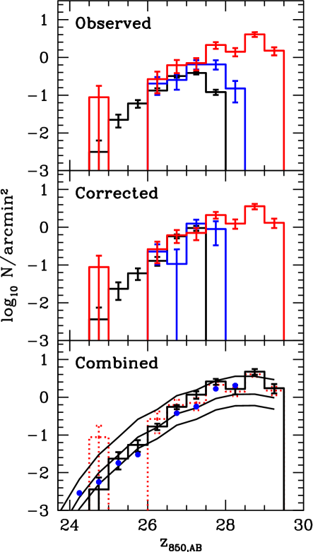
Figure 5.— Surface densities (per 0.5 mag interval) of $i$-dropouts observed at three different depths: GOODS (black histogram), HUDF-Ps (blue histogram), and HUDF (red histogram). Errors are the $1\sigma$ Poissonian uncertainties. The top panel presents the uncorrected surface densities. The middle panel presents these same surface densities, but corrected to the same level of completeness and flux biases as are present in the HUDF (Appendix D) and with the contaminants removed (note that incompleteness in the HUDF [or at HUDF depths] is accounted for using the selection volume, at a later stage: Figure 8). The bottom panel shows the cumulative surface density obtained by combining these fields through a maximum likelihood procedure (§3.8). The predicted surface densities of $i$-dropouts assuming the Steidel et al. (1999) LF, the Steidel et al. (1999) LF divided by 3, and the Steidel et al. (1999) LF divided by 6 are shown with the three solid black curves in the bottom panel. The uncorrected HUDF counts are also included in the bottom panel as the dotted red histogram. The equivalent differential counts of BSEM04 are included in this panel as blue circles (from their Figure 10). The no-evolution ($z\sim 3$) predictions exceed the observed counts by factors of $\approx 6$ at the bright end ($z_{850,AB}\lesssim 26$: Stanway et al. 2003, 2004b; Dickinson et al. 2004), $\approx 3$ at more intermediate magnitudes ($z_{850,AB}\sim 26-27$), and $\lesssim 2$ at faint end ($z_{850,AB}\gtrsim 27$). The effect of depth on the extracted counts is obvious in the top panel. A detailed quantification of the relevant biases (selection and measurement) is provided in Table D3 and Figure D2.

3.6. Field-to-Field Variations

The effective normalization of the luminosity function is expected to show significant variations as a function of position and environment ($\sim 35$% rms for single ACS pointings). This is the result of large-scale structure (loosely referred to as “cosmic variance”). Since the goal of these studies is to derive a luminosity function that is representative of the cosmic average, our challenge is to remove these variations. A simple averaging of the $i$-dropouts from the different fields is not appropriate since the fields differ in the magnitude ranges they probe. One would have no guarantee with such a procedure that the average normalization obtained at brighter magnitudes is the same as that obtained at fainter magnitudes, thus allowing for discontinuities in the normalization. This could impact the shape of the derived LF (see Appendix E).

To remove these differences, it is necessary to estimate the relative normalizations of $i$-dropouts in our different survey fields. We do this by degrading the deeper data to the depths of the shallower survey fields and then comparing the surface densities of $i$-dropouts derived. To maximize the significance, the present comparisons are done in two stages: (1) comparing the HUDF against the HUDF-Ps and (2) comparing the deeper three fields (HUDF + HUDF-Ps) against the GOODS fields. The overall normalization for our data sets is set by the mean of the two GOODS fields, which–sampling the largest comoving volume–should provide our best estimate of the cosmic average.

For the first stage, $i$-dropouts in the HUDF are normalized relative to $i$-dropouts in our deepest three fields. The normalization factor is determined by degrading the HUDF to the same S/N level as the two parallels and then comparing the number of dropouts in the fields. This degradation was performed 10 times and the S/N (weight maps) of both parallels were matched on a pixel-by-pixel basis (as in Appendix C and Appendix D1). Our findings are shown in Table 8 and point to the HUDF having a normalization similar to the first parallel (50.2 vs. 43.6), but substantially higher than that of the second parallel (27.8 vs. 11.4). Taken together, this suggests that the HUDF is 16$\pm$24% overdense relative to the mean of the HUDF-Ps, or 10$\pm$15% overdense relative to the cosmic average defined by the three fields. These fields also enable us to comment on the observed field-to-field variations, which appear to be $\sim$46% rms on $\sim 11$ arcmin² scales. This is consistent with the $\sim 35$% rms variations one obtains assuming a $\Lambda$CDM power spectrum, $\Delta z=0.7$ selection window, pencil beam geometry, and bias of 4, which is appropriate (Mo & White 1996) for objects of number density $\sim 10^{-3}$ Mpc^-3 probed by these fields (Figure 10).

Table 8Number of $i$-dropouts found in the two HUDF-Ps and in the HUDF degraded to the same depths.

	Number of dropouts
Field	HUDFP1	HUDFP2
HUDFP1	50.2	–
HUDFP2	–	11.4
HUDF	43.6	27.8

For the second stage, the normalization of the deeper three fields is adjusted to match that of the GOODS fields. As before, the normalization factor is estimated by degrading the HUDF and HUDF-Ps to the S/N level of the GOODS fields and extracting $i$-dropout samples using selection criteria identical to that used for GOODS. The results of these experiments are shown in Table 9, and it is clear that the average surface density derived from the three deeper fields ($0.69\pm 0.15\,\,\textrm{arcmin}^{-2}$) is somewhat lower ($0.70\pm 0.16$ times) than that found in both GOODS fields ($0.99\pm 0.06\,\,\textrm{arcmin}^{-2}$). $0.70\pm 0.16$ is the second stage normalization factor. Interestingly enough, the surface density of $i$-dropouts is 9% $\pm$ 13% larger in the CDF-S GOODS field than it is in the HDF-N GOODS field. However, this is not inconsistent with the sort of variations expected from cosmic variance ($\pm$20%) in fields of this size (160 arcmin²; Somerville et al. 2004). Multiplying the first and second stage factors together, we arrive at an overall normalization factor for the HUDF and HUDF-Ps. These factors are summarized in Table 10 under the “Two Stage” column.

Table 9Surface Densities of $i$-dropouts from different fields at GOODS depth.

	Surface Density
Field	(arcmin-2)
HDFN GOODS	0.94$\pm$0.08
CDFS GOODS	1.03$\pm$0.08
HUDFP1	0.78$\pm$0.28
HUDFP2	0.33$\pm$0.21
HUDF	0.97$\pm$0.29

As an alternative to this procedure, the normalization of our deeper fields can be derived by comparing directly with the surface density of $i$-dropouts found at GOODS depth (Table 9). Using the above results (i.e., Table 9), we derive a normalization of $0.98\pm 0.30$ and $0.56\pm 0.18$ for the HUDF and HUDF-Ps fields, respectively. These values are compiled under the “One Stage” column in Table 10. While consistent, they are of slightly lower significance than our estimates made with the two stage procedure. We adopt the results of the two stage procedure as our final estimate of the relative normalization and take the reciprocal of this normalization as our adjustment factor.

Table 10Adjustments made to the $i$-dropout surface densities from the different fields used in this study.

	Relative Normalization
Field	Two Stage	One Stage	Adjustment Factor
HUDFPs	$0.67\pm 0.16$	$0.56\pm 0.18$	1.50
HUDF	$0.77\pm 0.20$	$0.98\pm 0.30$	1.30
GOODS	1.0 (fixed)	1.0 (fixed)	1.00

3.7. Dependence of Galaxy Size on Redshift

Data from the HUDF, HUDF-Ps, and GOODS fields also allow us to revisit our analyses on the physical sizes of galaxies at $z\sim 6$ and how these sizes compare with those at latter times. Previously, we had carried out our analyses using each of the above fields separately (Bouwens et al. 2004b; Bouwens et al. 2004a; B06b). With the combined data set, we can significantly improve this analysis. For this paper, these sizes are important for modeling the selection effects of our $i$-dropout samples. Similarly to our previous work, we model the sizes of $i$-dropouts in all three samples using different size scalings $(1+z)^{-m}$ ($m$ = 0, 1, and 2) of a $z\sim 2.5$ HDF-N + HDF-S $U$-dropout sample (B06a). We project objects from this sample to higher redshift ($z\sim 5-7$) using our cloning software, add them to noise frames, and then reselect them in exactly the same way as the observed samples. Only galaxies 1 mag brightward of the selection limits are considered for our comparisons (to avoid being dominated by selection effects). Figure 6 for the $i$-dropouts from all three fields. Here it is evident that the typical half-light radius for $i$-dropouts at $z_{850,AB}\sim 27$ is 0.8 kpc (after correction for the PSF). Relative to the sizes of objects at lower redshift, the $(1+z)^{0}$ and $(1+z)^{-2}$ scalings seem to nicely bracket the observed range. To derive a more precise estimate, we rely on comparisons between the mean half-light radii obtained from the observations and simulations. Interpolating between our simulation results, our best-fit values for the size-evolution exponent $m$ are $1.2\pm 0.4$, $1.0\pm 0.5$, and $1.0\pm 0.4$ for the HUDF, HUDF-Ps, and GOODS fields, respectively. Combining the results from the three fields to obtain a single scaling (and thus assuming that this redshift scaling is luminosity independent) yields $m=1.1\pm 0.3$. This is in good agreement with several previous determinations: $m=[0.8,2.0]_{1\sigma}$ (B06b), $m=1.57_{-0.50}^{+0.53}$ (Bouwens et al. 2004a), $m=0.94_{-0.19}^{+0.25}$ (Bouwens et al. 2004b), and the Ferguson et al. (2004) $H(z)^{-1}$ size scaling, which is equivalent to $m=1.47$ over the redshift range $2.5<z<6$.

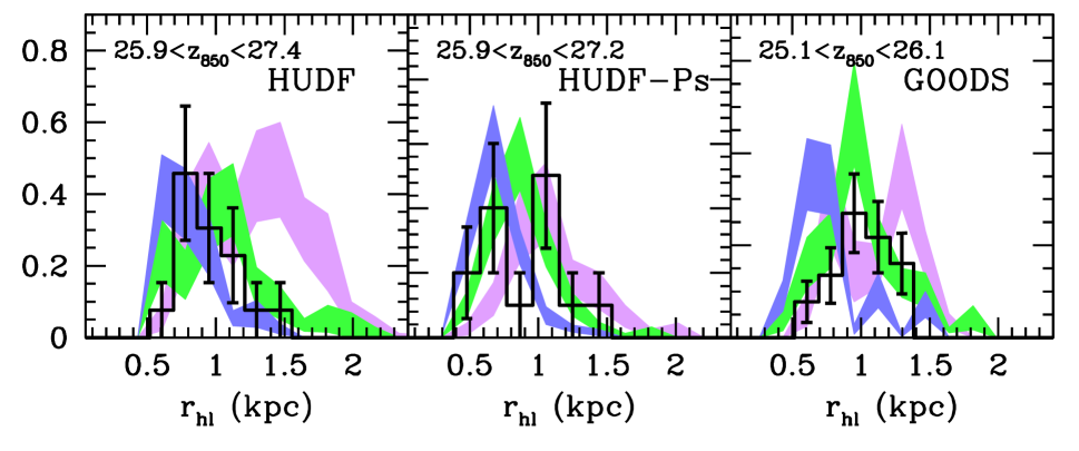
Figure 6.— Observed half-light radii (black histogram with $1\sigma$ Poisson errors) for a bright subset of $z\sim 6$ $i$-dropouts from the HUDF, HUDF-Ps, and GOODS fields vs. that predicted from $(1+z)^{0}$ (violet shaded region), $(1+z)^{-1}$ (green shaded region), and $(1+z)^{-2}$ (blue shaded region) size scalings of a $z\sim 2.5$ $U$-dropout sample from the HDF-N + HDF-S fields (B06a). The normalization is arbitrary. The breadth of the shaded regions indicates the $\pm 1\sigma$ uncertainties based on the finite size of our input samples (Bouwens et al. 1998a). Predictions for the GOODS data sets appear “noisy” due to the limited number of bright galaxies in our HDF-N+HDF-S input samples. The best-fit is obtained for a $(1+z)^{-1.1\pm 0.3}$ size scaling (see §3.7 for details). Typical $i$-dropouts at $z_{850,AB}\sim 27$ (from the HUDF-Ps and HUDF) have PSF-corrected half-light radii of $\sim 0.8$ kpc.

3.8. Best-Fit Surface Densities

It is useful to combine the results from our three data sets into a single measure of the $i$-dropout surface density as a function of magnitude. To derive this, we apply a maximum likelihood procedure. For all three data sets, the model counts are multiplied by the transfer functions (Appendix D3: from the HUDF to the relevant field), multiplied by the normalization factors from Table 10 (from the cosmic average to the normalization of the particular field), and then compared with the observed counts. In these fits, we do not include counts faintward of $z_{850,AB}=27.0$ in the two GOODS fields and faintward of $z_{850,AB}=28.0$ in the HUDF-Ps to be conservative. This allows us to avoid any systematics that may occur in modeling the selection effects near the completeness limit. The resulting surface density of $i$-dropouts is tabulated in the “I” column of Table 11 and shown in the bottom panel of Figure 5. This surface density spans 5 mag, running all the way from $z_{850,AB}\sim 24.5$ to 29.5. We remind the reader that the surface densities quoted here are as measured at HUDF depths and are not free of the incompleteness/flux biases implicit at these levels. Because of this, we have also included a second column in Table 11 that quotes the surface densities at HUDF depths corrected for blending with foreground objects (see Appendix D1).

Table 11$i$-dropouts surface densities estimated from HUDF, HUDF-Ps, and GOODS fields, corrected up to the HUDF completeness levels.

	Surface Density (arcmin-2)
Magnitude	I	II
$24.50<z_{850}<25.00$	$0.004\pm 0.004$	$0.004\pm 0.004$
$25.00<z_{850}<25.50$	$0.024\pm 0.011$	$0.028\pm 0.014$
$25.50<z_{850}<26.00$	$0.054\pm 0.019$	$0.066\pm 0.022$
$26.00<z_{850}<26.50$	$0.166\pm 0.033$	$0.201\pm 0.039$
$26.50<z_{850}<27.00$	$0.551\pm 0.071$	$0.664\pm 0.085$
$27.00<z_{850}<27.50$	$1.175\pm 0.265$	$1.416\pm 0.320$
$27.50<z_{850}<28.00$	$2.589\pm 0.478$	$3.119\pm 0.575$
$28.00<z_{850}<28.50$	$1.643\pm 0.456$	$1.980\pm 0.549$
$28.50<z_{850}<29.00$	$4.731\pm 0.797$	$5.701\pm 0.960$
$29.00<z_{850}<29.50$	$1.743\pm 0.481$	$2.100\pm 0.580$

4. Comparison With Previous Results

4.1. Source Lists and Surface Densities

In §3, we used $i$-dropouts measured at three different depths (GOODS, HUDF-Ps, and HUDF) to derive an optimal measure of the surface density of $i$-dropouts. Previously, there have been several attempts to compile the counts from these fields, and so it is useful to make comparisons with the source lists first before trying to understand possible differences in the interpretation. We begin with the $i$-dropouts from the HUDF, for which several source lists have already been compiled (BSEM04; Yan & Windhorst 2004b; Beckwith et al. 2006). Fortunately, these papers use selection criteria nearly identical to our sample, facilitating the comparisons. As far as the current catalogs are concerned, 48 of the 54 $i$-dropouts compiled by BSEM04 appear in our primary list (Table 4), four appear in our blended $z\sim 6$ candidate list (Table D4: see Appendix D1), one (BSEM04#49117) was blended with a foreground object in both our catalogs (Tables 4 and D4), and one (BSEM04#17487) had a $V_{606}$-band flux ($V_{606}-z_{850}=2.4$) inconsistent with our $i$-dropout selection criteria. Eighty-four of the brightest 95 $i$-dropouts ($z_{850,AB}<29.5$) from the Yan & Windhorst (2004b) catalog also appear in our primary list (Table 4), five appear in our blended $z\sim 6$ candidate list (Table D4), three had $V_{606}$-band fluxes inconsistent with our $i$-dropout criteria, and three were near the edges of the HUDF image and therefore outside our selection area. Possible differences in object splitting between catalogs are ignored in the above comparisons. As for the previously published catalogs, 35 of the brightest 39 $i$-dropouts from Table 4 ($z_{850,AB}<27.9$) appear in the BSEM04 catalog and 34 of these 39 appear in the Yan & Windhorst (2004b) compilation. Objects appear to be missing from the previous catalogs due to their surface brightness (e.g., as with HUDF-42566566 or HUDF-34998369), proximity to the $(i_{775}-z_{850})_{AB}=1.3$ color cut, and proximity to the edge of the HUDF frame, as is the case for HUDF-42209119 which is not given in the BSEM04 catalog.

In the GOODS fields, the surface densities we derive are less than those first reported by Giavalisco et al. (2004b) and Dickinson et al. (2004) using a similar $(i_{775}-z_{850})_{AB}>1.3$ selection on the three-epoch data. We obtain 0.10$\pm$0.02 and 0.30$\pm$0.05 arcmin^-2 to $z_{850,AB}\sim 26$ and 26.5, respectively, versus their surface densities of 0.17 and 0.37 arcmin^-2 to the same magnitude limits, after applying their estimated correction for contamination from photometric scatter (20%) and spurious fraction (23%). The disagreement becomes even worse, however, if an account is made for the fact that their surface densities derive from the three-epoch data (and would need to be corrected upward to account for the considerable incompletenesses at these depths). What is the source of this disagreement? A quick investigation suggests that it has come from a substantial underestimate of the contamination rate in these previous studies. Here we can revisit these estimates using the now deeper imaging data over the GOODS fields and in particular the HUDF-Ps and HUDF data. Of the 251 $i$-dropouts in the Dickinson et al. (2004) $i$-dropout catalog, only 12 overlap with the deeper HUDF (2 mag fainter) and HUDF-Ps (1 mag fainter) data. Three (25%) of these objects appear to be bona-fide $i$-dropouts, two (17%) are low-redshift interlopers, and seven objects (58%) are not found at all in the deeper data and therefore appear to be spurious. This works out to a 75% contamination rate, which is much higher than the $\sim$45% estimated in the Giavalisco et al. (2004b) and Dickinson et al. (2004) studies. To be fair, we note that these studies stressed the substantial uncertainties in their estimates. More striking is the fact that only 94 of the 251 $i$-dropouts in the Dickinson et al. (2004) catalog are even associated with real sources in our GOODS catalogs (based on data that are $\sim 0.7$ mag deeper in the $z_{850}$ band than that used by Dickinson et al. 2004) and just 48 of these appear to be bona-fide $i$-dropouts (Table 6). This suggests that the majority of objects in the original Dickinson et al. (2004) compilation were simply spurious sources. A cursory examination of these sources in the current ACS GOODS reduction bears out this supposition.

From the HUDF, BSEM04 made the point that the cumulative surface density of $i$-dropouts is only 0.1$\pm$0.1 arcmin^-2 to $z_{850,AB}\sim 26.5$. While the present results roughly corroborate this claim, we find a slightly higher density (0.30 arcmin^-2) to the same bright limit in our corrected counts (Table 11). The current value is a bit lower than the completeness corrected $0.5\pm 0.2$ $i$-dropouts arcmin^-2 cited in our earlier study on the RDCS1252-2927 + HDF-N fields (Bouwens et al. 2003b), but this appears to have been the result of large scale structure (B06a) and lensing by the prominent foreground cluster in that study. This surface density (0.30 arcmin^-2) also appears to be consistent with the three-epoch estimate from the GOODS team, if we assume the 75% contamination fraction derived earlier (and apply a small completeness correction).

4.2. Is the Surface Density of $i$-dropouts in the HUDF Typical?

The normalization of the $i$-dropout counts in a given field can show large variations (e.g., 35% rms for a single ACS field) depending on the large scale structure (“cosmic variance”). In §3.6, we are able to estimate the normalizations for our fields relative to the large area GOODS fields. One field that was of particular concern in this analysis was the HUDF because (1) it provides our best constraint on the number of faint $i$-dropouts and (2) it was selected to contain one particularly bright $z_{850,AB}=25.0$ $i$-dropout. Since rare objects are typically associated with overdensities, one might have expected the $i$-dropouts in the HUDF to be overdense relative to the cosmic average, compromising any LF we might have determined using its data.

In §3.6, we show that this is not likely an important concern, and that $i$-dropouts in the HUDF have a surface density that is just $0.76\pm 0.20$ times that of the two GOODS fields (and thus the HUDF may even be underdense relative to the cosmic average). Nevertheless, one might have expected this to be a concern given the recent findings by Malhotra et al. (2005) using the HUDF GRISM data. Comparing the redshift distribution of $i$-dropouts they observed with that obtained from their modelling, Malhotra et al. (2005) argued that the HUDF contained a factor of $\sim 2$ overdensity in the number of $i$-dropouts at $z=5.9\pm 0.2$ (15 of the total 23 $i$-dropouts). At first glance, these results may seem contradictory to our own, but one needs to remember that the Malhotra et al. (2005) measurement is really just a comparison between the volume density of $i$-dropouts inside the interval $z\sim 5.9\pm 0.2$ and that outside it. Since the comparison was made entirely within the area of the HUDF, it simply provides us with information on the large-scale structure at $z\sim 6$ along that line of sight.

5. Luminosity Function

The combined data from the HUDF, HUDF-Ps, and GOODS fields provide a unique opportunity to derive the luminosity function at $z\sim 6$ to unprecedented depths and accuracy. Such detail is important for making accurate inferences about galaxy evolution and the reionization of the universe. It allows us to address questions about the subsequent evolution of $UV$-bright galaxies to $z\sim 3$, indicating whether there has been evolution in $L_{*}$, $\phi^{*}$, or $\alpha$. It also allows us to make reliable estimates of the UV background produced by $z\sim 6$ galaxies. The UV background density is crucial for assessing the impact of $z\sim 6$ galaxies on reionization.

Estimating the LF would be straightforward if there were a simple way of converting the observed fluxes $m$ to an absolute magnitude $M$ that was essentially independent of redshift. Unfortunately, the $z_{850}$-band fluxes are heavily attenuated by the forest and thus conversions to absolute magnitude are highly dependent on the redshift of the source (see Figure 7). By contrast, our infrared fluxes–while not highly affected by the forest–are of much lower S/N and moreover are not available for many of our fields. As a result, our only recourse here is to use the $z_{850}$-band fluxes to work back to the absolute magnitudes through a modelling of the $i$-dropout redshift distribution. To do this, we consider an integral over the full redshift range in deriving the luminosity function $\phi(M)$:

$$\int_{z}\phi(M(m,z))P(m,z)\frac{dV}{dz}dz=N(m)$$ (1)

where $\frac{dV}{dz}$ is the cosmological volume element, $m$ is the apparent $z_{850}$-band magnitude, $N(m)$ is the number counts, $P(m,z)$ is the selection function, and $M$ is the absolute magnitude at 1350 $\AA$. The absolute magnitude $M$ is a function of both the apparent magnitude $m$ and redshift $z$.

Figure 7.— The $z_{850}$-band magnitude vs. redshift (thick solid line) for objects of a fixed luminosity (here a $L_{z=3}^{*}$ galaxy). Consequently, objects at a particular $z_{850}$-band magnitude can correspond to a wide range of luminosities (e.g., a $z_{850,AB}\sim 27$ $i$-dropout would correspond to a $0.3L_{z=3}^{*}$ object at $z\sim 5.5$ and a $2.5L_{z=3}^{*}$ object at $z\sim 7$). To cope with this issue, we model the redshift distribution and integrate the LF ($\phi_{k}$) over the relevant selection volume when fitting the observed counts $N_{m}$ (Eq. 5). One example of the effective kernel $V_{m,k}$ (Eq. 4) used in these integrations is shown here in the inset (for an object whose absolute magnitude corresponds to $L_{z=3}^{*}$). The effective kernels for other absolute magnitudes are similar. The vertical axis for the inset is in units of the selection volume per unit area per unit magnitude (Mpc³ arcmin^-2 mag^-1).

The selection function $P(m,z)$ can be estimated by projecting a complete $B$-dropout sample from the HUDF (Bouwens et al. 2004b) to $z\sim 5-7$ and reselecting it using a similar procedure to that described in §3.1. The projected $B$-dropout sample is assumed to have a $UV$-continuum slope $\beta$ with mean $-2.0$ and $1\sigma$ scatter of 0.5, similar to our fits in §3.4. It also makes sense to adopt a $(1+z)^{-1.1}$ size scaling (for fixed luminosity: §3.7). Motivated by the findings of Stanway et al. (2004a) and Dow-Hygelund et al. (2006), we also assume that 25% of the projected $B$-dropouts have Ly$\alpha$ emission with an equivalent width of $30\AA$. This latter assumption provides a rough account for the bias introduced by the current $(i_{775}-z_{850})_{AB}>1.3$ selection against galaxies with strong Ly$\alpha$ emission at $z\sim 5.5-5.9$ (Malhotra et al. 2005; Figure 6 of Dow-Hygelund et al. 2006). Since Ly$\alpha$ emission falls in the $i_{775}$ band for objects at these redshifts, such objects will not readily show up as dropouts. This reduces the selection volume for $z\sim 6$ galaxies by $\sim 3$%. The selection function we derive is shown in Figure 8.

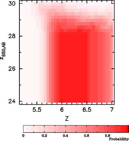
Figure 8.— Probability $P(m,z)$ that some object of apparent $z_{850,AB}$-band magnitude and redshift $z$ is included in our HUDF $i$-dropout sample. This function was computed by projecting a HUDF $B_{435}$-dropout sample (Bouwens et al. 2004b) to $z\sim 6$ assuming a $(1+z)^{-1.1}$ size scaling (for fixed luminosity: §3.7). Other scalings [e.g., $(1+z)^{-1}$ or $(1+z)^{-1.5}$] yield only modest differences with respect to the adopted selection function $P(m,z)$ and therefore only have a minor effect on the shape of the LF (e.g., $\Delta\alpha=\pm 0.1$). The rest-frame UV slopes $\beta$ of our input sample are assumed to have a mean of $-2.0$, with a $1\sigma$ scatter of 0.5. 25% of the objects are assumed to have a Ly$\alpha$ equivalent width of 30$\AA$ (Dow-Hygelund et al. 2006). This function does not include the small incompleteness ($\sim 11-17$%) due to blending with foreground sources (Appendix D1).

5.1. Direct Method

Here we present our primary determination of the rest-frame UV LF at $z\sim 6$. We express the LF in terms of a set of stepwise functions $\phi_{k}W(M-M_{k})$ of half-magnitude width:

$$\phi(M)=\Sigma_{k}\phi_{k}W(M-M_{k})$$ (2)

where

$$W(x)=\begin{array}[]{cc}0,&x<-1/4\\ 1,&-1/4<x<1/4\\ 0,&x>1/4\end{array}$$ (3)

We then derive the coefficients on the stepwise function through a maximum likelihood procedure, from a fit to the observed counts (Table 11). To simplify the computation, we derive kernels $V_{m,k}$ that convert the luminosity function $\phi_{k}$ to predicted counts:

$$V_{m,k}=\int_{z}\int_{m-1/4}^{m+1/4}W(M(m^{\prime},z)-M_{k})P(m^{\prime},z)\frac{dV}{dz}dm^{\prime}dz$$ (4)

With this definition, Eq. (1) reduces to

$$\Sigma_{k}\phi_{k}V_{m,k}=N_{m}$$ (5)

where $N_{m}=\int_{m-1/4}^{m+1/4}N(m^{\prime})dm^{\prime}$. One example of the kernel $V_{m,k}$ that appears in Eq. (4) is shown in Figure 7. Since our procedure here is essentially a deconvolution of $N_{m}$ (to obtain $\phi_{k}$), the LF we derive will have correlated errors. The LF will also appear somewhat more “noisy” than the original counts. As a result (and because of the Poissonian noise in the observed counts at $z_{850,AB}\gtrsim 27.5$), we have enlarged the size of our faintest two bins ($M_{1350,AB}>-19$) to be 1.0 mag in width. The resulting LF is shown in Figure 10 (see also Table 12) and extends over 2 orders of magnitude: from 4 $L_{z=3}^{*}$ to 0.04 $L_{z=3}^{*}$. Remarkably, this is fainter than what Steidel et al. (1999) was able to obtain at $z\sim 3$ (where the limit was $\approx 0.1L_{z=3}^{*}$). As a check on the current procedure, we repeated it on the surface density predictions made in Figure 5 (bottom) based on the $z\sim 3$ LF (Steidel et al. 1999) and were able to recover the input LF. For context, we present the predicted redshift distribution for this LF (and our HUDF $i$-dropout selection) in Figure 9.

Table 12A stepwise determination of the $z\sim 6$ rest-frame UV luminosity function (see also Figure 10).

$M_{1350,AB}$	$\phi_{k}$ (Mpc-3 mag-1)
$-21.94$	0.00001 $\pm$ 0.00001
$-21.44$	0.00007 $\pm$ 0.00004
$-20.94$	0.00012 $\pm$ 0.00007
$-20.44$	0.00033 $\pm$ 0.00012
$-19.94$	0.00128 $\pm$ 0.00030
$-19.44$	0.00313 $\pm$ 0.00118
$-18.69$	0.00332 $\pm$ 0.00115
$-17.69$	0.00771 $\pm$ 0.00211

In addition to breaking up the LF in stepwise intervals, it has also become conventional to parametrize it in terms of a Schechter function (Schechter 1976). Because of the degeneracies among the parameters $\alpha$, $\phi^{*}$, and $M^{*}$, the results are expressed as likelihood contours (Figure 11, blue solid lines). In deriving these contours, we allowed $\alpha$ to extend to values as steep as $-2$ to explore the broadest possible parameter space. Even though the luminosity density is formally divergent for such steep values of the faint-end slope, it seems clear that the LF must cut off at some physical scale and so the total light will not diverge. We evaluate the likelihood of different Schechter parametrizations by calculating the equivalent values of $\phi_{k}$ for the parametrization (by integrating the Schechter function over the full 0.5 mag interval relevant for the considered $\phi_{k}$), comparing them with the observed counts $N_{m}$ (Table 11) using Eq. (5), and then computing $\chi^{2}$. We have incorporated large-scale structure uncertainties into these likelihood estimates by smoothing the $\chi^{2}$ likelihood contours with a kernel that encapsulates the joint uncertainty in $\alpha$, $M^{*}$, and $\phi^{*}$ arising from field-to-field variations ($\sigma_{\alpha}=0.2$, $\sigma_{M^{*}}=0.14$, $\sigma_{\phi}=0.0006$, and their internal correlations: see Appendix E). An additional $\sim 20\%/\sqrt{2}\sim 14\%$ uncertainty in $\phi^{*}$ results from the expected field-to-field variations in the $i$-dropout surface densities over the two GOODS fields (Somerville et al. 2004; §3.6). To illustrate the effect of fixing the different Schechter parameters at the $z\sim 3$ values, green contours are overplotted in Figure 11. These results can be put in context by comparing them with the equivalent $z\sim 3$ determinations (Steidel et al. 1999). In the left two plots, we see evidence for lower characteristic luminosities $M^{*}$ at $z\sim 6$, with little change in $\phi^{*}$ or $\alpha$. Fainter values of $M^{*}$ are favored at 99.7% confidence. If we try to minimize changes in $M^{*}$, we can see that our results favor steeper values for $\alpha$ at $z\sim 6$. Note that scenarios, such as density evolution ($\phi^{*}$) which do not include these changes in $M^{*}$ (toward fainter values) or $\alpha$ (toward steeper values) are excluded at $>$99.99% confidence. Our most likely values for $\phi^{*}$, $M_{1350,AB}^{*}$, and $\alpha$ are $2.02_{-0.76}^{+0.86}\times 10^{-3}$ Mpc^-3, $-20.25\pm 0.20$, and $-1.73\pm 0.21$, respectively. As illustrated in Figure 10 (black line), this fit is in good agreement with the stepwise LF determined earlier (Table 12). Because of the proximity of the present faint-end slope to $-2$, where the integral of the total light diverges, extrapolations to zero luminosity can be somewhat uncertain. A much more robust number is the total luminosity density integrated to the approximate faint-end limit of the HUDF ($0.04L_{z=3}^{*}$): $1.77\pm 0.45\times 10^{26}\,\textrm{ergs}\,\textrm{s}^{-1}\,\textrm{Hz}^{-1}\,\textrm{Mpc}^{-3}$. This is equal to 0.68 times, 0.50 times, and 0.24 times the luminosity density integrated to zero assuming faint-end slopes $\alpha$ of $-1.6$, $-1.7$, and $-1.9$, respectively.

5.2. STY79 Method

A more conventional way of deriving the LF (across multiple fields) is to use the Sandage, Tammann, & Yahil (1979, hereafter STY79) fitting procedure. This procedure has the advantage of being relatively insensitive to large-scale structure. Only the shape of the luminosity function factors into the fits and not the normalization, allowing one to derive extremely robust measures on the overall shape. We do not use this procedure as our primary fitting procedure since our degradation procedure (§3.6) provides us with a slightly more direct measure of the field-to-field variance (the STY79 approach may be more sensitive to errors in our transfer functions). However, we show that the two results are in very good agreement, suggesting that our overall result here is robust.

As with our primary approach, an important complication is the rather inexact relationship between apparent and absolute magnitudes (Figure 7). This makes it more convenient to work in terms of the apparent rather than absolute magnitudes. Our procedure then becomes one in which we are maximizing the likelihood of producing the observed counts (here distributed over three different fields) given a LF. In detail, this approach really is not that different from what we performed in §3.6 to match up the counts from our three different data sets, and so it should not be surprising that the best-fit parameters we obtained from this procedure (i.e., $M^{*}_{1350,AB}=-20.28$ and $\alpha=-1.74$) and their likelihood contours (Figure 12) are in good agreement with those obtained with our primary methodology (Figure 11). The $\phi^{*}$ we derive fixing the shape of the LF and fitting to the number counts in the two GOODS fields (Figure 5, middle) is $1.94\times 10^{-3}$ Mpc^-3 and also quite consistent.

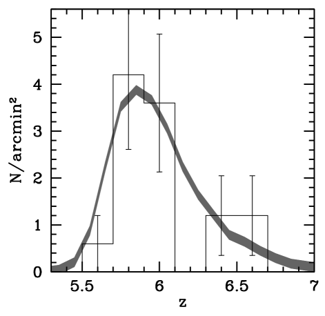
Figure 9.— Redshift distribution of $i$-dropouts in our HUDF selection assuming the $z\sim 6$ LF from Figure 10 and a mean rest-frame UV continuum slope $\beta$ of $-2.0$ with a $1\sigma$ scatter of 0.5 (shaded gray region). Object profiles used in the simulations were drawn from comparable luminosity HUDF $B$-dropouts (Bouwens et al. 2004b) scaled in size as $(1+z)^{-1.1}$ (§3.7). Our predicted redshift distribution is in good agreement with that obtained by Malhotra et al. (2005) for $i$-dropouts from the HUDF [histogram: clipped to include only objects with $(i_{775}-z_{850})>1.3$ and with a vertical normalization scaled to match our predictions]. This suggests that our model for the rest-frame $UV$-colors of the $z\sim 6$ galaxy population is reasonable. It may also indicate that Malhotra et al. (2005) overestimated the size of the overdensity at $z\sim 5.9\pm 0.2$ in the HUDF.

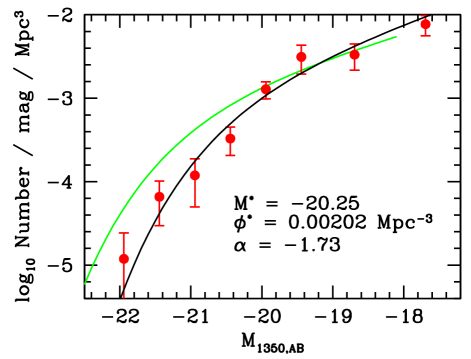
Figure 10.— Rest-frame continuum $UV$ ($\sim 1350\AA$) LF estimated from the HUDF, the HUDF-Ps, and the GOODS fields, shown in terms of the best-fit stepwise parameterizations (red circles with $1\sigma$ errors; see Table 12) and Schechter function (black line). Because of the greater noise in the $i$-dropout counts at $z_{850,AB}\gtrsim 27.5$, the LF is binned on 1.0 mag intervals faintward of $M_{1350,AB}=-19$ (otherwise 0.5 mag intervals are used). Note that adjacent bins in our LF are not independent [see Eq. (1) and Figure 7], and therefore the errors on the individual bins include some covariance with their neighbors. The $z\sim 3$ Steidel et al. (1999) LF (with the $k$-corrected equivalent $M_{1350,AB}^{*}=-20.87$, see Table 13) is shown for comparison (green line) and only plotted to its faint-end limit $0.1L_{z=3}^{*}$. Amazingly, this is brighter than the faint-end limit we were able to obtain at $z\sim 6$ (0.04 $L_{z=3}^{*}$). Our $z\sim 6$ LF shows a clear turnover at the bright end relative to the $z\sim 3$ LF and suggests that there has been an evolution in the characteristic luminosity from $z\sim 6$ to 3 ($\sim 0.6$ mag of brightening: see also Figure 11).

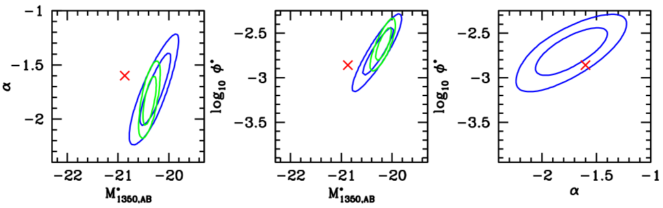
Figure 11.— Maximum likelihood Schechter parameters ($M^{*}$, $\alpha$, and $\phi^{*}$) for the $z\sim 6$ UV ($\sim 1350\AA$) luminosity function. The inner and outer contours indicate the 68% and 95% confidence regions, respectively. The blue contours indicate the confidence intervals after marginalizing across the third parameter in the LF. The green contours show these confidence intervals if no change is allowed in this third parameter from $z\sim 3$ (Steidel et al. 1999). The red cross indicates the parameters for the $z\sim 3$ Steidel et al. (1999) LF shifted to 1350 $\AA$ rest frame. Note that even though the luminosity density is formally divergent for faint-end slopes $\alpha<-2$, it seems clear that the LF must cut off at some physical scale and so the total light will not diverge. We considered such steep slopes to explore the broadest possible parameter space. The simplest way to accommodate the observed evolution is to shift the characteristic luminosity $M^{*}$ by $\sim 0.6$ mags (brightward) from $z\sim 6$ to 3 although an evolution in the faint-end slope $\alpha$ (from $-1.9$ at $z\sim 6$ to $-1.6$ at $z\sim 3$) can also help. LFs that do not include these changes (a fainter $M^{*}$ or a steeper $\alpha$ at $z\sim 6$) are excluded at $>$99.99% confidence.

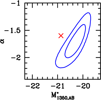
Figure 12.— Maximum likelihood Schechter parameters ($M^{*}$, $\alpha$) for the $z\sim 6$ UV ($\sim 1350\AA$) luminosity function. This figure is similar to the left-hand panel of Figure 11, but using the maximum likelihood procedure of Sandage et al. (1979). The results here are in excellent agreement with those obtained with the direct method (§5.1: Figures 10-11)

5.3. Direct Method (without LSS correction)

Finally, it is interesting to compute the $z\sim 6$ LF but without any correction for large-scale structure (“cosmic variance”). Since field-to-field variations (i.e., 35% rms for a single ACS field: §3.6) are only slightly larger than our measurement errors on these variations (the uncertainties on the normalization factors for the HUDF are 26% rms: see Table 10), the LF we derive ignoring the normalization altogether (i.e., assuming each field is representative of the cosmic average) should be fairly competitive with our primary determination (§5.1). Meanwhile, differences we observe relative to this determination can provide us with a good sense for the representative errors. Rederiving the LF with these assumptions, we obtained the following best-fit Schechter parameters: $\phi^{*}=1.76\times 10^{-3}$ Mpc^-3, $M_{1350,AB}^{*}=-20.28$, and $\alpha=-1.60$. It is encouraging that these values are only slightly different from those obtained from the two previous methods (Figures 11 and 12). In retrospect, we might have expected this level of agreement from some simulations we ran to assess the impact of cosmic variance on the derived LF (Appendix E).

5.4. Luminosity Densities

Having obtained a basic fit to the observed LF, we can move on to look at the UV continuum luminosity density and how it compares with previous determinations at higher and lower redshift. Because of the limited sensitivies of the highest redshift probes (e.g., the Bouwens et al. 2004c study at $z\sim 7-8$ and the Bouwens et al. 2005 study at $z\approx 10$), we make these comparisons to two different luminosity limits: 0.3 times and 0.04 times the characteristic luminosity at $z=3$ (Steidel et al. 1999). This is important to properly account for possible evolution in the characteristic luminosity $L^{*}$ or faint-end slope $\alpha$ with redshift. To a limiting magnitude of $0.3L_{z=3}^{*}$, the present LF integrates out to $5.8\pm 0.9\times 10^{25}\,\textrm{ergs}\,\textrm{s}^{-1}\,\textrm{Hz}^{-1}\textrm{Mpc}^{-3}$.

To convert these UV luminosity densities into star formation rate (SFR) densities (uncorrected for extinction), we assume a Salpeter IMF and use the now somewhat canonical conversion factors of Madau et al. (1998):

$$L_{UV}=\textrm{const}\,\,\textrm{x}\,\,\frac{\textrm{SFR}}{M_{\odot}\textrm{yr}^{-1}}\textrm{ergs}\,\textrm{s}^{-1}\,\textrm{Hz}^{-1}$$ (6)

where const = $8.0\times 10^{27}$ at 1500 $\AA$. Both the present luminosity densities and SFR densities are shown in Figure 13 relative to many previous determinations (Steidel et al. 1999; Giavalisco et al. 2004b; Bouwens et al. 2004a, 2004c, 2005; BSEM04; Schiminovich et al. 2005). The fall off in the luminosity density towards high redshift is much sharper at brighter luminosities [$>0.3L_{z=3}^{*}$; $\rho(z=6)/\rho(z=3)=0.52\pm 0.08$] than it is when integrated to $0.04L_{z=3}^{*}$ [$\rho(z=6)/\rho(z=3)=0.82\pm 0.21$].

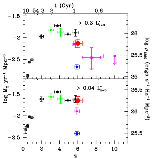
Figure 13.— Cosmic star formation history (uncorrected for extinction) integrated to $0.3L_{z=3}^{*}$ (top panel) and $0.04L_{z=3}^{*}$ (bottom panel). These luminosities correspond to the faint-end limits for $z_{850}$ and $i_{775}$-dropout probes at $z\sim 7-8$ and 6, respectively. The large red circle denotes the current determination at $z\sim 6$. A Salpeter IMF was used to convert the rest-frame continuum $UV$ luminosity density ($\sim 1350\AA$) to a SFR density. For comparison, the previous determinations by Schiminovich et al. (2005; open hexagons), Steidel et al. (1999; green crosses), Giavalisco et al. (2004b; black diamonds), Bouwens et al. (2004a; magenta triangle), BSEM04 (blue square), Bouwens et al. (2004c; magenta pentagon: shifted slightly to the left in the upper panel to avoid confusion), and Bouwens et al. (2005; magenta square) are also included. The age of the universe is plotted along the top. The plotted position of the BSEM04 $z\sim 6$ determination is as quoted in their paper (although our own fits to the BSEM04 counts yield values $\sim 2.7$ times higher; §6.1). The Giavalisco et al. (2004b) $z\sim 6$ determination appears to have been significantly affected by contamination (§4.1). The figure is divided into two panels to illustrate how much stronger the evolution is at the bright end of the LF ($\gtrsim 0.3L_{z=3}^{*}$) than it is when integrated to the faint-end limit of the current probe ($0.04L_{z=3}^{*}$).

6. Discussion

The combination of the HUDF, HUDF-Ps, and GOODS datasets, especially the very deep HUDF data, provides a unique opportunity to explore a number of issues for $z\sim 6$ galaxies. These include refining our knowledge of the rest-frame $UV$-continuum luminosity function, assessing the impact of $z\sim 6$ galaxies on the reionization of the universe, and using $z\sim 6$ as a baseline for assessing evolution to even higher redshift. Our analysis of the rest-frame $UV$-colors also permits us to revisit the issue of a possible evolution in the $UV$-continuum slope $\beta$.

6.1. UV Continuum Luminosity Function

One of the principal goals of this paper is to obtain an optimal determination of the luminosity function in the rest-frame continuum UV ($\sim 1350\AA$). The present approach has several important advantages over several previous derivations (Dickinson et al. 2004; Yan & Windhorst 2004a, 2004b; Bouwens et al. 2004a; BSEM04; Malhotra et al. 2005). These include obtaining a self-consistent selection of $i$-dropouts from three of the deepest, widest area data sets (GOODS, HUDF-Ps, and HUDF); systematic use of the deeper ACS and infrared data to derive completeness, flux, and contamination corrections; use of the average UV continuum colors in our selection volume estimates; an inclusion of the selection biases against strong Ly$\alpha$ emitters in these same selection volume estimates; and a detailed matching-up of the surface density of $i$-dropouts in our deeper fields with that obtained in shallower, wider area fields to ensure a proper normalization of the overall LF.

The current refinement to the $z\sim 6$ LF puts us in a good position to examine several previous determinations of this LF and the associated claims for evolution from $z\sim 3$ (Dickinson et al. 2004; Yan & Windhorst 2004a, 2004b; Bouwens et al. 2004a; BSEM04; Malhotra et al. 2005). A summary of many previous Schechter parameterizations are given in Table 13 and plotted relative to the current determination in Figure 14. We divide this discussion between the bright and faint ends of the LF. At the bright end ($M_{1350,AB}\lesssim-21$), we find a substantial (factor of $\sim 6$) deficit relative to the $z\sim 3$ LF. This supports the initial findings of Stanway et al. (2003, 2004b) and Dickinson et al. (2004). Our current estimate for the number density of $i$-dropouts at the bright end is slightly smaller than what we reported in two previous studies (Bouwens et al. 2003b, 2004a). In the first case this was because of a substantial (factor of $\approx 2$) overdensity in the RDCS1252-2927 field relative to the cosmic average (§4.1; B06a) and in the second case it was because of slight ($\sim 20$%) overestimates of the surface densities and completeness present in the GOODS fields (Bouwens et al. 2004a). The number density is also less than reported by Yan & Windhorst (2004b). This appears to have been due to their reliance on the three-epoch GOODS $i$-dropout catalog (Dickinson et al. 2004) which, as we discuss earlier (§4.1), overestimates the surface density of $i$-dropouts. Recent searches at bright magnitudes ($z_{R,AB}<25.6$) with Subaru also find strong ($\approx 11$ times) deficits at $z\sim 6$ relative to $z\sim 3$ values (Shimasaku et al. 2005).

Table 13Determinations of the best-fit parameters for the rest-frame UV ($\sim 1350\AA$) LF at $z\sim 6$.

Study	$M_{1350,AB}^{*}$	$\phi^{*}$ (Mpc-3)	$\alpha$
This work	$-20.25\pm 0.20$	$0.00202_{-0.00076}^{+0.00086}$	$-1.73\pm 0.21$
Dickinson et al. 2004	$-19.87$	0.00527	$-1.6$ (fixed)
Bouwens et al. 2004a	$-20.26$	0.00173	$-1.15$
Bunker et al. 2004	$-20.87$	0.00023	$-1.6$
Yan & Windhorst 2004b	$-21.03$	0.00046	$-1.8$
Malhotra et al. 2005	$-20.83$	0.0004	$-1.8$ (assumed)

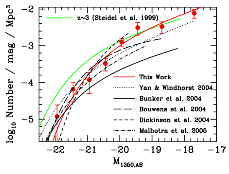
Figure 14.— Comparison of our rest-frame continuum UV ($\sim 1350\AA$) luminosity function (Figure 10; red line and red circles) with that of others. Included are the $z\sim 6$ LFs of Yan & Windhorst (2004; dotted black line), BSEM04 (thin solid black line), Bouwens et al. (2004a; thick dashed black line), Dickinson et al. (2004; thin dashed black line), and Malhotra et al. (2005; dashed-dotted line). The $z\sim 3$ Steidel et al. (1999) LF shifted to 1350 $\AA$ rest-frame is shown for context (green line). All the LF determinations are only plotted to their nominal faint-end limits. A compilation of the Schechter parameterizations of the plotted LFs is provided in Table 13. The careful and comprehensive nature of the current analysis should make the present determination of the $z\sim 6$ LF the most robust (§6.1).

At fainter luminosities, the $z\sim 6$ LF shows much better agreement with $z\sim 3$ than at the bright end. This suggests evolution. As discussed earlier (§5), the simplest way to accommodate these changes is through an evolution of the characteristic luminosity (99.7% confidence). Our best-fit is a $0.6\pm 0.2$ mag brightening in $M^{*}$. An evolution of the faint-end slope $\alpha$ to $-1.9$ can also help (from $-1.6$ at $z\sim 3$: Steidel et al. 1999). The latter option echoes earlier claims made by Yan & Windhorst (2004b) for a steep faint-end slope ($\alpha=-1.8$) using data from the HUDF. However such faint-end slopes do not appear to be required (Figure 11). The faint-end slope is nevertheless steeper than the $\alpha=-1.15$ determined in our earlier work using the HUDF-Ps (Bouwens et al. 2004a). The shallower slope from that study appears to have derived from the significantly lower surface density of $i$-dropouts present in the HUDF-Ps ($\sim 0.6$ times the cosmic average: see Table 10). Contrary to this work (§3.6), no attempt was made there to treat possible field-to-field variations, and therefore the shape of the LF was affected. The Dickinson et al. (2004) determination, by contrast, was too high at lower luminosities. This appears to have been a consequence of their substantial underestimate of the contamination rate (§4.1).

Our determination also differs substantially from the best-fit LF of BSEM04 (Figure 14), particularly at the faint end where our LF is nearly a factor of $\sim$10 higher. Since the derived counts from BSEM04 are only slightly lower than those in our study (Figure 5), how can the differences in the LF be so large? The volume element does not appear to be the culprit since the BSEM04 no-evolution predictions from $z\sim 3$ (Steidel et al. 1999) closely match our own. The only possible explanation appears to be due to some peculiarity in the way that BSEM04 derived their best-fit parameters. From their figures 10 and 11, it would appear that BSEM04 conducted their fits ($\chi_{r}^{2}$) on the cumulative counts, not the differential counts. If so, this would not be appropriate as the data points in the cumulative counts are not independent. Our own fits to their differential counts (Figure 5, blue circles) yield $M_{1350,AB}^{*}=-20.49$ and $\phi^{*}=0.00097$ assuming a fixed $\alpha=-1.6$. This fit gives a cumulative luminosity density to their faint-end limit ($z_{850,AB}=28.5$) which is $\sim 2.7$ times higher than their optimal fit (a factor of $\approx 6$ drop in $\phi^{*}$ from $z\sim 3$).

The Bunker et al. (2004) work excepted, there has been a growing consensus among $z\sim 6$ studies that the evolution in the UV LF at high redshift occurs primarily at the bright end. Shimasaku et al. (2005) made a similar argument based on a comparison of their bright $i$-dropout search with those obtained at fainter magnitudes (Bouwens et al. 2004a; Bunker et al. 2004; Yan & Windhorst 2004b). Such luminosity-dependent trends would also partially explain the supposed discrepancy (e.g., Trimble & Schwanden 2005; Stanway et al. 2004b) between several early $z\sim 6$ results, in which different evolutionary factors were quoted relative to no-evolution $z\sim 3$ expectations (e.g., $\approx 6$ by Stanway et al. 2003 vs. $\approx 2$ by Bouwens et al. 2003b). Although it was previously believed that these differences might be due to uncertainties in the completeness and contamination rates (Bouwens et al. 2003b; Stanway et al. 2004b), it now appears that differences in the flux limit may have played an equally important role.

It seems relevant to step back and look at the observed evolution in the larger context of galaxy evolution. What is remarkable about the evolution we observe is that the characteristic luminosity of galaxies in the UV shows a significant increase over the range $z\sim 6$ to 3. This is in contrast to the strong decrease observed from $z\sim 2$ to 0 (Arnouts et al. 2005; Gabasch et al. 2004) and suggests that galaxy formation is a very different process early on than it is at much later times. At early times, it seems reasonable to imagine that this increase in luminosity we observe is just a simple consequence of the merging and coalescence of galaxies expected in hierarchical scenarios. The fact that this does not occur at later times suggests that something must halt this growth and even turn it around. Although we discuss it no further, two promising explanations for this turn-around include active galactic nucleus (AGN) feedback (e.g., Scannapieco et al. 2005; Croton et al. 2005; Granato et al. 2004; Scannapieco & Oh 2004; Binney 2004; Di Matteo et al. 2005) and the transition from cold to hot flows (e.g., Birnboim & Dekel 2003).

In light of the likely relationship between the luminosity evolution observed and the evolution of the mass function, it makes sense to examine this connection briefly. Figure 15 presents the mass function at $z\sim 3$ and 6 calculated from the Sheth & Tormen (1999) formalism and a $\Lambda$CDM power spectrum (Bardeen et al. 1986) with $\sigma_{8}=0.9$, $\Omega_{b}=0.045$, $\Omega_{M}=0.3$, $\Omega_{\Lambda}=0.7$, and $H_{0}=70\,\textrm{km/s/Mpc}$. A horizontal blue arrow is overplotted to indicate the approximate mass range of dropouts which make up the current LF (e.g., Cooray 2005). Two aspects are evident in the evolution of the mass function: (1) halos of a given density are $\sim 2-3$ times more massive at $z\sim 3$ as at $z\sim 6$ and (2) the slope of the mass function becomes shallower with time ($\Delta\alpha=0.27$ from $z\sim 6$ to $z\sim 3$). The first change is very similar to $\sim 0.6$ mag (factor of $\approx 2$) brightening of the LF observed here. The second change–this trend toward shallower faint-end slopes–is less clear from current data (cf. Yan & Windhorst 2004b), but will almost certainly be tested in the near future. Similarities between the observed evolution and predictions for the mass function suggests that we are actually observing hierarchical growth over the range $z\sim 6$ to 3 (see e.g., Cooray 2005 and Night et al. 2005 for more sophisticated treatments).

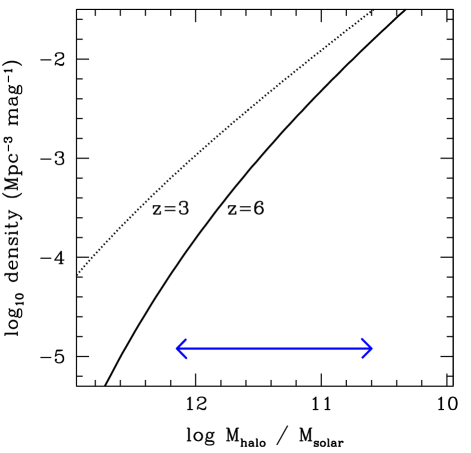
Figure 15.— Mass function (comoving volume density) at $z\sim 3$ (dotted line) and $z\sim 6$ (solid line) calculated using the Sheth & Tormen (1999) formalism and a $\Lambda$CDM power spectrum (Bardeen et al. 1986) with $\sigma_{8}=0.9$, $\Omega_{b}=0.048$, $\Omega_{M}=0.3$, $\Omega_{\Lambda}=0.7$, and $H_{0}=70\,\textrm{km/s/Mpc}$. The horizontal blue arrow provides the likely mass range for $i$-dropouts in our sample (e.g., Cooray 2005). Besides an obvious evolution toward higher masses at later times (factor of $\approx 3$ change), the mass function is also expected to flatten ($\Delta\alpha=+0.27$ from $z\sim 6$ to 3).

6.2. Rest-frame UV colors

The present sample also allowed us to place constraints on the mean redshift and rest-frame UV slope $\beta$. We obtained these constraints using the measured optical-infrared colors for specific $i_{775}$-dropouts from the HUDF (Table 4). A comparison of our measured colors with those obtained in two previous studies (Stanway et al. 2005; Yan & Windhorst 2004b) shows no large systematic differences, but considerable scatter ($\pm 0.15$ mag) for individual objects. The scatter becomes even larger ($>0.4$ mag) in cases of possible blending with foreground objects. Relative to previous measurements, we would expect our measurements to represent a modest improvement given our use of more optimized scalable apertures (thus avoiding most blending problems) and careful aperture corrections.

Despite no large systematics relative to previous measurements of the colors, the mean $\beta$ inferred in this study is $-2.0$, which is redder than the $\beta=-2.2$ inferred in the Stanway et al. (2005) study based on the same data. The principal reason for the difference here is that current inferences are based on the $J-H$ colors while previous inferences were based on the $z-J$ colors. Since the $z-J$ colors are highly influenced by the redshift of a source and moreover can be quite insensitive to rest-frame UV color (see B06a), it is better to use the $J-H$ colors to determine the rest-frame $UV$ slope. The $z-J$ colors are also more sensitive to errors in image alignment, errors in the aperture corrections, and uncertainties in the optical to infrared zero points. Therefore, we consider the present determination to be an improvement on the Stanway et al. (2005) estimate (though current uncertainties in the zero points may make all present measures somewhat uncertain, i.e., $\Delta\beta=\pm 0.3$: §2.1).

Irrespective of the exact $\beta$, the mean rest-frame UV slope observed at $z\sim 6$ is bluer than that observed at $z\sim 3$. This evolution is consistent with a number of recent studies (Lehnert & Bremer al. 2003; Kneib et al. 2004; B06a; Bouwens et al. 2004c; Schaerer & Pelló 2005; Yan et al. 2005; cf. Ouchi et al. 2004) and point towards a lower mean dust extinction at higher redshift. Changes in age, metallicity, and the IMF have a much smaller effect on the rest-frame UV slope (e.g., Schaerer 2003; Leitherer et al. 1999). Moreover, a significant contribution from Ly$\alpha$ to the $J_{110}$ flux seems unlikely given constraints from emission line searches at $z\sim 6$ (Ajiki et al. 2003; Kodaira et al. 2003; Hu et al. 2004; BSEM04; Stanway et al. 2004a; Nagao et al. 2004; Dow-Hygelund et al. 2006). This leaves an evolution in the dust content as the most natural way of explaining this change (see also the discussion in B06a).

One obvious consequence of this lower dust extinction is an evolution in the correction factor applied to the SFR densities inferred directly from the UV luminosity function (see also B06a; B06b; Stanway et al. 2005). A convenient way of estimating the effect of this change is through the Meurer et al. (1999) fit relating the extinction $A_{1600}$ to the UV slope $\beta$: $A_{1600}=4.43+1.99\beta$. Although there is some uncertainty in the exact value of $\beta$ at $z\sim 6$ (and $z\sim 3$), it is useful to adopt some fiducial value of $\beta$ to estimate the size of the effect. Taking $\beta$ to equal $-2.0$ at $z\sim 6$ and $-1.5$ at $z\sim 3$ (Adelberger & Steidel 2000) suggests a doubling of the attenuation factor at $1600\AA$ from $z\sim 6$ to $z\sim 3$. Since this is the same direction as the evolution of the UV LF, it appears that the real evolution (after correction for extinction) may be large indeed. So, instead of the factor of 2 increase in the characteristic luminosity from $z\sim 6$ to 3 inferred in Figure 11, the real evolution in this quantity may be as large as a factor of $\sim 4$ increase after correction for extinction. It may also suggest that the total SFR (and UV luminosity) density at $z\sim 6$ (after correction for extinction and integrated to $0.04L_{z=3}^{*}$) is just $\sim 0.3$ times the value at $z\sim 3$ (instead of the 0.82 factor given in §5.4). We have included a simple illustration of this effect in Figure 16 using several representative determinations of the UV luminosity density (Steidel et al. 1999; Schiminovich et al. 2005). The dust corrections we have applied here are $\sim 2$ times (0.4 mag) at $z\sim 6$ and otherwise from Schiminovich et al. (2005). As is apparent from the figure, such changes have wide-range implications and indicate a much more rapid rise in the corrected star formation history from $z\sim 6$ to $z\sim 3$ than in the uncorrected SFR density. Clearly, it will be important to confirm this change with other methods (e.g., by using stacked X-ray fluxes: Reddy & Steidel 2004; Lehmer et al. 2005).

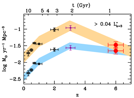
Figure 16.— Cosmic star formation history integrated to $0.04L_{z=3}^{*}$. This history is shown both with and without extinction corrections (upper and lower points, respectively). This is also indicated by the orange and light blue shaded regions, respectively, where the width here gives the suggested uncertainties (see Schiminovich et al. 2005). Similar to Figure 13, we use the Madau et al. (1998) prescription to convert luminosity densities into SFR densities. Included are the determinations of Schiminovich et al. (2005; hexagons), Steidel et al. (1999; dark magenta crosses), and the present $z\sim 6$ determinations (red circles). The extinction corrections we apply at low redshift ($z\lesssim 3$) are $\sim 1.4$ mag and are intermediate between the high and low estimates given in Schiminovich et al. (2004; i.e., 1.8 and 1.0, respectively). The extinction correction we infer at $z\sim 6$ is a significantly smaller $\sim 0.4$ mag (from the Meurer et al. 1999 prescription). Evolution in the extinction correction over the range $z\sim 3-6$ appears to have a substantial impact on the cosmic star formation history (§6.2).

As we conclude this section, perhaps we should not be surprised by this evolution in the rest-frame UV slope or the dust extinction. Given the strong correlation between the total SFRs and the dust extinction (Wang & Heckman 1996; Martin et al. 2005; Adelberger & Steidel 2000), we might have expected the extinction to be lower at the highest redshifts. The mass scales are expected to be lower there, and as we have observed, so are the typical UV luminosities and apparent SFRs.

6.3. Reionization of the Universe

In light of the observational evidence that $z\sim 6$ marks the end of the reionization epoch (Becker et al. 2001; Fan et al. 2002; White et al. 2003), it has become common to use the observed $i$-dropouts to comment on the possible reionization of the universe by photons arising from galaxies (e.g., Stanway et al. 2003, 2004b; Lehnert & Bremer 2003; Bouwens et al. 2003b; Giavalisco et al. 2004b; Dickinson et al. 2004; BSEM04; Stiavelli et al. 2004b; Yan et al. 2004a,b). An estimate of the star formation rate necessary to produce this reionizing flux can be made using the convenient formulation of Madau et al. (1999) modified to match the baryon density derived from the one-year WMAP results (Spergel et al. 2003) and shifted to $z\sim 6$ (Bouwens et al. 2003; BSEM04):

$$\dot{\rho_{*}}\approx(0.052\,\,{\rm M_{\odot}\,yr^{-1}\,Mpc^{-3}})\,\left(\frac{0.5}{f_{\rm esc,rel}}\right)\,C_{30}\left(\frac{1+z}{7}\right)^{3}.$$ (7)

where $\dot{\rho_{*}}$ is the SFR density, $C_{30}$ is the H $\scriptstyle\rm I\$ clumping factor $\left\langle\rho_{\hbox{H~{}$\scriptstyle\rm I\ $}}^{2}\right\rangle$/$\left\langle\rho_{\hbox{H~{}$\scriptstyle\rm I\ $}}\right\rangle^{2}$ / 30, and $f_{\rm esc,rel}$ is the relative fraction of ionizing radiation escaping into the intergalactic medium to that escaping in the $UV$-continuum ($\sim 1500\AA$). Unfortunately, current constraints on the total SFR $\dot{\rho_{*}}$ still remain poor. Although an integration of our best-fit LF to our faint-end limit and zero luminosity yields 0.022 and 0.043 $\,\,{\rm M_{\odot}\,yr^{-1}\,Mpc^{-3}}$, respectively (somewhat smaller than the fiducial SFR needed), current constraints also allow for substantially steeper values of the faint-end slope (e.g., $\alpha\sim-1.9$: Figure 11). Such slopes would nearly double the value of $\dot{\rho_{*}}$ and hence be sufficient to reionize the universe in this formulation. Of course, it is also true that physical constraints become important for some faint-end slope (given limits on the total stellar mass or metals produced, e.g., Madau et al. 1998, Stiavelli et al. 2004a).

Despite current refinements to the $z\sim 6$ UV continuum LF, there continue to be substantial uncertainties in the role that $z\sim 6$ galaxies play in reionizing the universe. Indeed, we should not forget that we still do not have a direct measure of the ionizing radiation escaping into the intergalactic medium (IGM) and are forced to rely on a proportionality factor, called the relative escape fraction, to convert the observed rest-frame continuum-UV flux into an ionizing flux. While most attempts to measure this escape fraction at $z\lesssim 3$ have thusfar only obtained upper limits (i.e., $<0.1$ to $<0.4$) (Leitherer et al. 1995; Hurwitz et al. 1997; Deharveng et al. 2001; Giallongo et al. 2002; Fernández-Soto et al. 2003; Malkan et al. 2003; Inoue et al. 2005), there have been other notable efforts (e.g., Steidel et al. 2001) that have obtained much larger values ($\gtrsim 0.5$). The situation remains somewhat controversial. As a result of these and other uncertainties (e.g., Stiavelli et al. 2004b), there has been a wide range of different claims regarding the capacity of galaxies to reionize the universe. Some authors have claimed that the observed galaxies are not sufficient to reionize the universe (BSEM04) while others have claimed that they are, either because of a higher ionizing efficiency (Stiavelli et al. 2004b) or because of a large contribution from lower luminosity galaxies at the faint end of the luminosity function (Yan & Windhorst 2004a, 2004b). This study (with its more rigorous and detailed matching up of the different surveys) provides an important confirmation and extension of this latter result, although it is not yet clear that the faint-end slope is unusually steep (i.e., $\alpha\lesssim-1.8$: as argued by Yan & Windhorst 2004a, 2004b). This being said, we would like to reemphasize the considerable uncertainties present at this stage and how little knowledge we have about how the escape fraction might behave, both in its redshift and in its luminosity dependence. Better constraints will be available when we are able (1) to better characterize the escape fraction and (2) to look at the ionizing flux of $z\gtrsim 3$ objects more directly (as one might obtain through proximity studies).

6.4. Implications for $z_{850}$-dropout Samples

Our redetermination of the $z\sim 6$ LF allows us to remark on recent $z\sim 7.5$ $z_{850}$-dropout samples selected from the HUDF. There are two recent samples that are relevant: the Yan & Windhorst (2004b) sample and the Bouwens et al. (2004c) sample. Yan & Windhorst (2004b) performed a shallow search for $z$-dropouts ($J_{110,AB}\lesssim 26.6$) and found only one candidate, which was just on the edge of their selection window. Since they predicted 2.9 candidates to a similar limit from their $i$-dropout LF assuming no-evolution, they interpreted this as a tentative indication for the onset of galaxy formation at $z\sim 6$. Performing a much deeper search ($H_{160,AB}<27.5$) on the same field, Bouwens et al. (2004) found five such $z_{850}$-dropout candidates, four of which they assume to be real in their fiducial estimates (at least one was considered to be spurious due to the aggressive nature of the search). Comparing this with the 14 $z_{850}$-dropouts predicted assuming no-evolution from $z\sim 4$, this appeared consistent with a factor of $\sim 3-5$ drop in the number (luminosity density) of $UV$-bright objects from $z\sim 4$ to 7.5.

It is relevant to revisit these issues using the $z\sim 6$ LF. Comparisons can be made by projecting the present $i$-dropout sample to $z\sim 6-9$ using our cloning software, adding it to the data and then reselecting it. In simulating the profiles of specific $i$-dropouts in our LF, we use scaled versions of specific $i$-dropouts from the HUDF matched to the current $i$-dropout LF (Appendix F of B06a details an anologous modelling of $U$-dropouts using the HDF profiles). Running through this procedure, 0.8 $z_{850}$-dropouts are expected to $J_{110,AB}\sim 26.6$ versus the one found, and 6.6 $z_{850}$-dropouts are expected to $H_{160,AB}\sim 27.5$ versus the four fiducial candidates. This suggests that there has only been a modest increase in the number of bright objects from $z\sim 7-8$ to 6, although the uncertainties are large due to small number statistics, cosmic variance, and some questions about the $z_{850}$-dropout candidates themselves (items 2b, 2c, and 2f from Bouwens et al. 2004c).

7. Conclusions

We have compiled a sample of 506 $i$-dropouts ($z\sim 6$ galaxies) from the HUDF, the HUDF parallel ACS fields (HUDF–Ps), and the GOODS fields (316 arcmin²), the latter enhanced by the ACS supernova search data (extending the depth of the ACS $i$ and $z$-data by 0.2 and 0.4 mag, respectively, to the depth of the ver. 2.0 GOODS release). This statistically robust sample consists of 122, 68, and 332 galaxies, respectively, from the three aforementioned fields and includes objects as faint as $z_{850,AB}\sim 29.5$. Note that 16 of these $i$-dropouts appear in more than one of the above samples. The current sample of 506 galaxies represents the most comprehensive and robust compilation to date, and is a significant advance over the $\sim$50 and $\sim$100 object sample assembled by Bunker et al. (2004) and Yan & Windhorst (2004b) over the HUDF, the 30 object sample obtained by Bouwens et al. (2004a) over the HUDF-Ps, and the 251 object sample that Dickinson et al. (2004) compiled from GOODS, although the latter sample is largely composed of contaminants ($\sim$75%: see §4.1).

Table 14Properties of $z\sim 6$ Galaxies.

Parameter	Value
$r_{hl}$ (at $z_{850,AB}\sim 27$)	$\sim$0.8 kpc ($\sim 0.14^{\prime\prime}$)
Size-Redshift Scaling	$(1+z)^{-1.1\pm 0.3}$
UV slope $\beta$	$-2.0\pm 0.3$
$\phi^{*}$	$0.00202_{-0.00076}^{+0.00086}$ Mpc-3
$M_{1350,AB}^{*}$	$-20.25\pm 0.20$
$\alpha$	$-1.73\pm 0.21$
${\cal{L}}_{1350}(>0.3L_{z=3}^{*})$	$5.8\pm 0.9\times 10^{25}\,\textrm{ergs/s/Hz/Mpc}^{3}$
${\cal{L}}_{1350}(>0.04L_{z=3}^{*})$	$1.77\pm 0.45\times 10^{26}\,\textrm{ergs/s/Hz/Mpc}^{3}$

We select these galaxies using the well–established dropout technique, with an $i$–dropout criterion [$(i_{775}-z_{850})_{AB}>1.3$, $(V_{606}-z_{850})_{AB}>2.8$] and demonstrate that the contamination levels on our selection are $\lesssim 8$% (i.e., $\gtrsim 92$% are real: Appendix D4).

Contamination is a potentially serious concern for dropout samples. We gave particular attention to four sources of contamination: intrinsically red low–redshift galaxies, stars, spurious sources, and low–redshift galaxies scattering into the selection region (photometric scatter). We established the contamination levels by performing object selection in degraded versions of the deepest fields, and used the deep (NICMOS) and wide-area (ISAAC) infrared images of these fields. As we discuss in Appendix D4.1, red galaxies only appear to be a significant source of contamination ($18_{-9}^{+13}$% of our $i$–dropout candidates) at bright magnitudes ($25<z_{850,AB}<26$) and again possibly at the faintest magnitudes ($10_{-5}^{+8}$%: $z_{850,AB}\gtrsim 28$). Contamination from photometric scatter is also small ($<$10%) and only important near the faint-end limit. Contamination from stars is uniformly low at all magnitudes ($\lesssim 3$%; after filtering out the few obvious bright cases), while that from spurious sources is insignificant. Overall, the present $i$–dropout catalogs are extremely clean ($\lesssim 8$% contamination).

An optimal measure of the $i$-dropout surface densities over a 5 mag range ($24.5<z_{850,AB}<29.5$) is determined from our three samples (HUDF, HUDF–Ps, enhanced GOODS). Detailed degradation experiments are made on our deeper data sets in order to understand object selection and photometry in our shallower fields and to derive completeness, flux and contamination corrections. These corrections are applied to establish a common baseline across all data sets. To remove the effects of large-scale structure (we expect $\sim$35% rms variations in the surface density of $i$-dropouts over 11.3 arcmin² ACS fields) when combining our three $i$-dropout samples, we carefully match up the surface density of $i$-dropouts in the deeper HUDF and HUDF-Ps probes to that found in the two enhanced wide-area GOODS fields (§3.6). The HUDF and HUDF–Ps fields are underdense ($0.77\pm 0.20$ times and $0.67\pm 0.16$ times) relative to the cosmic average defined by the two GOODS fields (Table 10).

Finally, we use our derived surface densities to calculate a rest-frame UV LF at $z\sim 6$, and compared this LF with lower redshift ($z\sim 3$) LFs. Quantitative estimates of both the sizes and UV colors of objects in our samples are used to estimate accurate selection volumes for the derived LF. Our principal findings are summarized in Table 14 and are as follows:

Galaxy sizes: Typical $i$-dropouts at $z_{850,AB}\sim 27$ (from the HUDF-Ps and HUDF) have PSF-corrected half-light radii of $\sim 0.8$ kpc or $\sim 0.14^{\prime\prime}$ (Figure 6: §3.7). By comparing the observed sizes of $i$-dropouts from our three different data sets with that predicted using different scalings of a $z\sim 2.5$ $U$-dropout sample (B06a), we make inferences about how the physical sizes of galaxies depend on redshift (for fixed luminosity). Our best-fit is a $(1+z)^{-1.1\pm 0.3}$ scaling, which is in good agreement with several previous determinations (Ferguson et al. 2004; Bouwens et al. 2004a,b; B06b).

Rest-frame UV colors / UV-to-total SFR correction: By modelling the $z-J_{110}$ and $J_{110}-H_{160}$ colors of $i$-dropouts from the NICMOS HUDF (see §3.3), we construct models for the rest-frame UV colors of the $i$-dropout population and the redshift distribution (which we find peaks at $z\lesssim 6$ – see also Malhotra et al. 2005). The mean rest-frame UV spectral slope $\beta$ we infer is $-2.0$. This is bluer than the $-1.5$ observed at $z\sim 3$ (Adelberger & Steidel 2000), but redder than the Stanway et al. (2005) estimate of $\beta=-2.2$ at $z\sim 6$ using the same data. A similar evolution from bluer spectral slopes has already been noted in a number of other high-redshift ($z>3$) studies (Lehnert & Bremer 2003; Kneib et al. 2004; B06a; Bouwens et al. 2004c; Schaerer & Pelló 2005; Yan et al. 2005; cf. Ouchi et al. 2004). The most natural explanation for this evolution is an increase in the dust content at later cosmic times. The most salient implication of such an evolution is the effect it would have on the inferred SFR densities. Using the Meurer et al. (1999) relation between the $UV$ slope $\beta$ and the extinction $A_{1600}$, we estimate this factor (at $1600\AA$) to change (in linear units) from $\sim 2$ at $z\sim 6$ to $\sim 4$ at $z\sim 3$.

Luminosity Function: Using the surface densities of $i$-dropouts from our data sets and a computed selection function $P(m,z)$, we derive the rest-frame continuum UV ($\sim 1350\AA$) LF at $z\sim 6$ from $4L_{z=3}^{*}$ to $0.04L_{z=3}^{*}$ ($M_{1350,AB}\sim-17.5$: see §5). This is fainter than Steidel et al. (1999) was able to obtain at $z\sim 3$ ($0.1L_{z=3}^{*}$). The likelihood parameters we derive for different Schechter parameterizations suggest that there has been an increase in the characteristic luminosity $M_{1350,AB}^{*}$ from $z\sim 6$ to 3 (99.7% confidence). The best-fit is a $0.6\pm 0.2$ mag brightening. This evolution in $M^{*}$ can be partially offset by changes in the faint-end slope $\alpha$ (from $-1.9$ at $z\sim 6$ to $-1.6$ at $z\sim 3$; Steidel et al. 1999). Scenarios, such as density evolution ($\phi^{*}$), which do not include this evolution in $M^{*}$ or $\alpha$ are excluded at $>$99.99% confidence, demonstrating quite significantly that galaxies at $z\sim 6$ have lower luminosities (on average) than galaxies at $z\sim 3$. The best-fit Schechter parameters are $M_{1350,AB}^{*}=-20.25\pm 0.20$, $\alpha=-1.73\pm 0.21$, and $\phi^{*}=2.02_{-0.76}^{+0.86}\times 10^{-3}$ Mpc^-3. We note that the best-fit parameters are $M_{1350,AB}^{*}=-20.31\pm 0.20$ and $\phi^{*}=1.80_{-0.68}^{+0.77}\times 10^{-3}$ Mpc^-3 if we express them using the cosmological parameters $(\Omega_{M},\Omega_{\Lambda},h)=(0.24,0.76,0.73$) preferred by the one year WMAP measurements (Spergel et al. 2003).

Luminosity/SFR density: The rest-frame continuum UV ($\sim 1350\AA$) luminosity density at $z\sim 6$ is $5.8\pm 0.9\times 10^{25}\,\textrm{ergs/s/Hz/Mpc}^{3}$ integrated to $0.3L_{z=3}^{*}$ and $1.77\pm 0.45\times 10^{26}\,\textrm{ergs/s/Hz/Mpc}^{3}$ integrated to $0.04L_{z=3}^{*}$ (§5). This is $0.52\pm 0.08$ times and $0.82\pm 0.21$ times, respectively, the luminosity density at $z\sim 3$ (Steidel et al. 1999) to comparable faint-end limits. The large dispersion in previous results at $z\sim 6$ seems at least in part to have been due to a dependence on the faint-end limit (e.g., compare the panels in Figure 13). Adopting the evolution in the UV-to-total correction factors quoted earlier (and thus dust content as the reason for the change in the rest-frame UV colors), we infer a much stronger evolution in the SFR density over the range $z\sim 6$ to 3 than is found in the luminosity density. Using the Meurer et al. (1999) prescription, we estimate that the SFR density at $z\sim 6$ is only $\sim 0.3$ times that at $z\sim 3$ (to $0.04L_{z=3}^{*}$), quite different from the change in the luminosity density (i.e., $\sim 0.82$ times).

Reionization of the universe: Assuming an escape fraction of 0.5 and H $\scriptstyle\rm I\$ clumping factor of 30, we estimate that a SFR density of 0.052 $\,\,{\rm M_{\odot}\,yr^{-1}\,Mpc^{-3}}$ is needed to reionize the universe using the Madau et al. (1999) formulation (§6.3). This is to be compared to the 0.022 $\,\,{\rm M_{\odot}\,yr^{-1}\,Mpc^{-3}}$ observed to the limit of our probe and the 0.043 $\,\,{\rm M_{\odot}\,yr^{-1}\,Mpc^{-3}}$ obtained by extrapolating our best-fit LF to zero luminosity. Despite being lower than the fiducial SFR densities required, there are sufficient uncertainties at present (particularly in the escape fraction, ionizing efficiency, and faint-end slope) that this factor of 2 difference is not significant. $z\sim 6$ galaxies seem capable of reionizing the universe (see also Stiavelli et al. 2004b; Yan & Windhorst 2004a,b).

$z\sim 7-8$ galaxies: Projecting the present $i$-dropout LF to $z\sim 6-9$, we make an estimate of the number of $z_{850}$-dropouts that would have been found in a number of recent work (Yan & Windhorst 2004b; Bouwens et al. 2004c). We estimate 0.8 $z_{850}$-dropouts to $J_{110,AB}\sim 26.6$ versus the one found by Yan & Windhorst (2004) and 6.6 $z_{850}$-dropouts to $H_{160,AB}\sim 27.5$ versus the four fiducial candidates found in the Bouwens et al. (2004c) study. Despite substantial uncertainties, this suggests that the rest-frame UV LF only shows a slight change from $z\sim 6$ to 7.5 (§6.4).

The HST ACS data from the HUDF, HUDF-Ps and GOODS fields (enhanced by the extensive supernova search data) enabled us to detect 506 $z\sim 6$ galaxies. This significant sample has been used to derive a rest-frame $UV$ luminosity function at $z\sim 6$ that extends 3 mag below $L^{*}$ (to 0.04$L^{*}$), as well as to provide improved constraints on size and color evolution, clearly establishing that galaxies are smaller and bluer at earlier times. The $z\sim 6$ LF demonstrates that the brightest galaxies are less luminous at $z\sim 6$, i.e., that luminosity evolution is the dominant characteristic of the evolving galaxy population between $z\sim 6$ (0.9 Gyr) and $z\sim 3$ (2 Gyr). The broad consistency of these results with the expectations of hierarchical models is encouraging. However, it is the quantitative constraints made possible with current data sets that are really important. Like $z\sim 3$, $z\sim 6$ seems destined to become an important reference point in our studies of galaxy evolution, marking the end of the reionization epoch and providing a useful baseline for theoretical exploration to even earlier times.

Appendix A $V-z$ Color Cut

While $i-z$ color criterion is quite effective at isolating $z>5.5$ galaxies, a more robust selection is possible using the $V$-band fluxes. This takes advantage of our expectation that the $V$-band fluxes of galaxies at $z>4$ will be highly attenuated by the Ly$\alpha$ forest. However, we cannot simply demand that our $z\sim 6$ candidates have no detectable ($<2\sigma$) $V$-band flux. This is because of the residual transmission at $\lambda\sim 912-1216\AA$ (incomplete Gunn-Peterson trough) which allows several of the brighter $z\sim 6$ galaxies in the HUDF to show faint $V$-band detections. Therefore, we must arrive at some criterion which allows for some $V$-band flux in our $z\sim 6$ selection, but not too much. The criterion we settled upon was $(V_{606}-z_{850})_{AB}>2.8$ color cut (Figure A1) for our high redshift selection. Although ideally this criterion would have provided a clean separation between the low-redshift interlopers and high redshift objects (i.e., $z>5.5$), such a separation isn’t entirely possible. Excluding all low-redshift objects would require the cut to be 3.5 (Figure A1), while including the bluest objects to $z\sim 5.5$ would nominally require the cut to be 2.9 (although a consideration of the photometric scatter, typically $\gtrsim 0.4$ mag, suggests that 2.5 would be better). Therefore, it was necessary for us to settle on some compromise between 2.5 and 3.5. After some experimentation, we chose 2.8.

We note that interlopers not identified with our $(V_{606}-z_{850})_{AB}<2.8$ criterion should be identified using the red-galaxy criterion $(z_{850}-K_{s})_{AB}>1.6$ in Appendix D4.1 or using the photometric scatter experiments (Appendix D4.2) where the $V-z$ colors of the undegraded galaxies in those experiments are known very well.

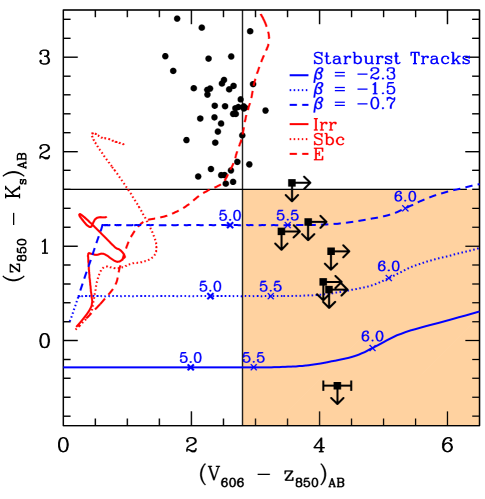
Figure 17.— Motivation for our $(V_{606}-z_{850})_{AB}>2.8$ cut used for selecting $i$-dropouts. The measured $(V_{606}-z_{850})_{AB}$ / $(z_{850}-K_{s})_{AB}$ colors for spectroscopically confirmed $i_{775}$-dropouts (squares: Dickinson et al. 2004; Malhotra et al. 2005) are contrasted with those obtained from a set of lower redshift interlopers selected in the CDF-S GOODS ISAAC footprint (circles; Table 2). The latter objects were selected to have $(i_{775}-z_{850})_{AB}$ colors redder than 1.0 and $(z_{850}-J)_{AB}$ colors redder than 0.8. The model colors are shown for three different UV spectral slopes $\beta$ and three different low-z interlopers (Coleman et al. 1980). Redshifts are marked on the diagram alongside the tracks. The $(V_{606}-z_{850})_{AB}=2.8$ color cut shown here (vertical line) is used to discriminate against low-$z$ early types and all later spectral types that enter into our sample (see Appendix A). Early-types not caught by the $(V_{606}-z_{850})$ cut will be included in our estimates of the contamination fraction using the $z_{850}-K_{s}$ colors of objects from the CDF South GOODS ISAAC and HUDF NICMOS data (see Figure D3, Table D7, and Appendix D4.1). Red $(i_{775}-z_{850})_{AB}>1.3$ objects with $(z_{850}-K_{s})_{AB}>1.6$ colors (horizontal line) are included in this contamination fraction.

Appendix B Degradation Procedure

At several points in our analysis, we found it convenient to degrade our deeper data to some shallower S/N level. In §2.3, we used this procedure to obtain a uniform S/N level across the two GOODS fields, and in §3.4, §3.6, Appendix C, and Appendix D, we used this procedure to quantify the effect of S/N on object selection and photometry.

Before discussing our degradation procedure, it is helpful to provide some background on both our noise models and weight maps, which are expressed in units of the inverse variance (equal to what they would be without any correlation in noise). To determine the noise model for each of our images, we measure the rms variance in apertures of different sizes, and then find an rms noise level and noise kernel that reproduced the observed variation in rms noise as a function of aperture size. The best fit noise levels were then used to scale the weight (inverse variance) maps provided with the HUDF (Beckwith et al. 2006) or obtained from our “apsis” software (Blakeslee et al. 2003).

By comparing the weight maps on our deeper data with that desired for our degradation experiments, we determined how much noise needed to be added to each pixel. We then made simple realizations of this noise and smoothed these realizations with the appropriate noise kernels to obtain the correct correlation properties. Finally, we added this noise to our deeper data and updated the pixel-by-pixel weights to reflect the lower S/N levels.

Appendix C Degradation Experiments

To assess the completeness, contamination rate, and flux measurements in our shallower fields relative to our deeper fields, we degraded our deeper fields (HUDF and HUDF-Ps) to the depths of our shallower fields (HUDF-Ps and GOODS) in a series of experiments. These degradations provide a very natural way of estimating the effect that photometric scatter has on both our selection and measurement process. Experiments included degrading the UDF to the depth of the first HUDF parallel (HUDFP1), degrading the UDF to the depth of the second HUDF parallel (HUDFP2), degrading the UDF to the depth of the GOODS fields, degrading HUDFP1 to the depth of the GOODS fields, and degrading HUDFP2 to the depth of the GOODS fields. Each degradation was repeated 10 times to minimize the dependence on any particular noise realization. To maximize realism, we ensured that the pixel-by-pixel weight maps of the degraded images were identical to those of the shallower fields. This was of particular interest for the HUDF-Ps (§2.2) because the depth in these fields varies by $\sim 0.4$ mag across the field of view. Then, $i$-dropouts were selected using the selection criteria of our shallower fields. Our degradation procedure is detailed in Appendix B.

Objects obviously associated with the diffraction wings of stars or bright elliptical galaxies were eliminated to mimic the selection procedure used for the main catalog (where similar spurious sources were eliminated). Objects selected by this procedure were divided into two categories: contaminants and $z\sim 6$ objects. Objects with $(V_{606}-z_{850})_{AB}$ colors bluer than 2.8 were classified as contaminants and objects with $(V_{606}-z_{850})_{AB}$ colors redder than 2.8 were classified as $z\sim 6$ objects (see Appendix A). In a few cases, where it was clear that the $V$-band photometry was contaminated by a nearby foreground object, we reclassified what would otherwise be labeled a contaminant as a $z\sim 6$ $i$-dropout. Despite some ambiguity regarding the exact split between the two categories, our results are not expected to depend on the exact split chosen. More stringent $(V_{606}-z_{850})_{AB}$ cuts will result in a higher contamination rate for the shallower field, but this will be offset by a lower selection volume.

Appendix D Corrections Applied to Our Data

This section describes the corrections we applied to the surface densities of $i$-dropouts derived from our shallower data in order to put them on a similar footing to our deeper HUDF data. These corrections compensate for the greater incompleteness levels, flux biases, and contamination expected to be present in the shallower data.

We start by looking at what can be said about the completeness levels and flux biases by degrading the available data. Although these issues are best treated with transfer functions (Appendix D3), our initial analyses here provide some valuable benchmarks that we can use later to assess the validity of the transfer functions we determine.

D.1. Completeness Corrections

A generic consequence of S/N thresholds and standard detection algorithms is an overall incompleteness at faint magnitudes and large sizes. An illustration of this is provided in Figure D1 for the three fields under study. It is immediately apparent that the distribution of $i$-dropouts in the HUDF, HUDF-Ps, and GOODS fields do not extend much to the upper-right of the three 50% completeness contours shown. As a result, significant incompleteness is not expected until at least $z_{850,AB}\sim 26.8$ in the GOODS fields, $z_{850,AB}\sim 27.5$ in the HUDF-Ps fields, and $z_{850,AB}\sim 29$ in the HUDF.

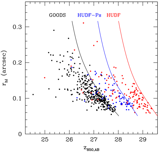
Figure 18.— Size-magnitude diagram for $i_{775}$-dropouts from the HUDF (red dots), HUDF-Ps (blue dots), and GOODS fields (black dots). Size is presented here in terms of the half-light radius. The 50% completeness limits (solid lines) are overplotted for the three fields and assume an $r^{1/4}$ surface brightness profile. These limits were determined by laying down galaxies of different sizes and total magnitudes on a noise frame and then attempting to recover them with our selection procedure (§3.1). By comparing the size-magnitude distribution of objects from our deeper surveys with our shallower surveys, it is obvious that significant incompleteness only sets in beyond $z_{850,AB}\sim 26.8$ in the GOODS fields and $z_{850,AB}\sim 27.5$ in the HUDF-Ps. A more detailed quantification of these biases is provided in the text and Table D3 (see also Bouwens et al. 2004b).

Perhaps the most model-independent way of estimating the incompleteness in our shallower fields relative to the HUDF is to degrade the deeper data sets to the same S/N as these shallower fields and then repeat the selection procedure. The very similar PSFs, pixel sizes, and passbands for all data sets considered here make this a straightforward process. The deeper data also provide a natural way of determining the fraction of objects on the degraded frames that are high redshift objects and the fraction of objects that are likely contaminants or noise. These simulations are described in Appendix C.

By comparing the surface density of the sources recovered in the deeper images with that recovered at the shallower depths (while excluding those objects whose $V_{606}$-band fluxes indicate they might be contaminants, Appendix D4.2), we are able to compute the completeness for the different fields under study. The results of the simulations are given in Tables D1-D2 and can be put together to obtain an estimate of the completeness relative to the HUDF.

Table 15Number of $i$-dropouts from the HUDF (11 arcmin²) recovered at the depths of our shallower two data sets.

Magnitude Interval	GOODS	HUDF-Ps	HUDF
$24.5<z_{850,AB}<25.0$	1.0	1.0	1
$25.0<z_{850,AB}<25.5$	0.0	0.0	0
$25.5<z_{850,AB}<26.0$	0.0	0.0	0
$26.0<z_{850,AB}<26.5$	2.7	2.9	3
$26.5<z_{850,AB}<27.0$	3.1	7.0	7
$27.0<z_{850,AB}<27.5$	1.8	7.9	8
$27.5<z_{850,AB}<28.0$	0.6	13.7	24
$28.0<z_{850,AB}<28.5$	0.0	4.9	16
$28.5<z_{850,AB}<29.0$	0.0	2.8	46

Table 16Number of $i$-dropouts from the HUDF-Ps (17 arcmin²) recovered at the depths of the GOODS fields.

Magnitude Interval	GOODS	HUDF-Ps
$24.5<z_{850,AB}<25.0$	0.0	0
$25.0<z_{850,AB}<25.5$	0.0	0
$25.5<z_{850,AB}<26.0$	0.0	0
$26.0<z_{850,AB}<26.5$	2.0	3
$26.5<z_{850,AB}<27.0$	2.4	3
$27.0<z_{850,AB}<27.5$	2.9	15
$27.5<z_{850,AB}<28.0$	1.1	15
$28.0<z_{850,AB}<28.5$	0.1	29
$28.5<z_{850,AB}<29.0$	0.0	3

An application of binomial statistics to the results of Table D1 enables a fairly straightforward determination of the magnitude-dependent completeness of the HUDF-Ps relative to the HUDF. While a similar procedure can be used to calculate the completeness of the GOODS probe relative to the HUDF, tighter constaints can be obtained by using objects from both the HUDF (Table D1) and HUDF-Ps (Table D2). This takes advantage of the fact that the HUDF-Ps are significantly more complete than the GOODS fields are. However, to use the results from the HUDF-Ps, we need to make a small correction for the small differences in the completeness between the HUDF and HUDF-Ps selections (based on the results in Table D1). The $1\sigma$ confidence intervals on the incompleteness of both fields are tabulated in Table D3.

Table 17The Relative Completeness of the shallower data sets to the HUDF.

Magnitude Interval	GOODS (OBS)	GOODS(SIM)	HUDF-Ps (OBS)	HUDF-Ps (SIM)
$24.5<z_{850,AB}<25.0$	$>0.56$	0.98	$>0.56$	1.00
$25.0<z_{850,AB}<25.5$	–	0.92	–	0.99
$25.5<z_{850,AB}<26.0$	–	0.86	–	0.98
$26.0<z_{850,AB}<26.5$	$0.77_{-0.17}^{+0.13}$	0.79	$0.97_{-0.24}^{+0.03}$	0.98
$26.5<z_{850,AB}<27.0$	$0.55_{-0.14}^{+0.14}$	0.63	$>0.87$	0.90
$27.0<z_{850,AB}<27.5$	$0.22_{-0.07}^{+0.10}$	0.32	$0.99_{-0.12}^{+0.01}$	0.86
$27.5<z_{850,AB}<28.0$	$0.04_{-0.02}^{+0.04}$	0.05	$0.57_{-0.10}^{+0.10}$	0.61
$28.0<z_{850,AB}<28.5$	$<0.03$	0.00	$0.31_{-0.10}^{+0.11}$	0.28
$28.5<z_{850,AB}<29.0$	$<0.02$	0.00	$0.06_{-0.03}^{+0.04}$	0.04

Finally, we discuss issues of incompleteness due to blending with foreground sources (object overlap). Although not generally considered to be an important source of incompleteness ($\lesssim 10$%) for HST studies, here blending played a slightly larger role. This was due to our choice of blending parameters (DEBLEND_MINCONT=0.15), which we adopted to ensure that SExtractor kept many of the more lumpy dropouts in our sample in a single piece (see §3).

To compute the incompleteness from blending, we included $i$-dropouts from our samples onto the image frames, and then attempted to recover them with our selection procedure. We used analytic versions (i.e., best-fit exponential profiles) of these dropouts in the simulations to avoid introducing additional noise onto the image frames. To control for possible incompleteness from photometric scatter and surface brightness selection effects, we also laid down dropouts on empty frames. The net increase in incompleteness due to the presence of foreground objects is approximately 17%, 10%, and 8% for $i$-dropouts in our HUDF, HUDF-P, and GOODS fields, respectively. These numbers appear to be relatively insensitive to the flux of the source.

As a basic check on these results and to see how much our incompleteness determinations were affected by our choice of deblending parameters, we experimented with a smaller value for the deblending parameter (DEBLEND_MINCONT=0.0001) using the HUDF data. With this choice, we calculated an incompleteness of 11%, again using the above procedure. Since this is smaller than what we calculated for our fiducial parameters (17%), we should find more dropouts in the HUDF with these parameters. In fact, nine additional $i$-dropouts (Table D4) were found. This increase (from 122 to 131) is almost exactly what we would have expected by comparing the incompleteness results for the two different values of DEBLEND_MINCONT (i.e., 11% vs. 17%).

Table 18$i$-dropouts in the HUDF which were blended with foreground sources in our main HUDF catalog (Table 4).

								$r_{hl}$
Object ID	R.A.	Decl.	$z_{850}$	$i-z$	$z-J$	$J-H$	S/G	(arcsec)
HUDF-38397588	03:32:38.39	-27:47:58.8	26.94$\pm$0.04	1.3	-0.2	0.0	0.02	0.14
HUDF-36458342	03:32:36.45	-27:48:34.2	27.25$\pm$0.06	1.3	$<$-0.1	faint	0.01	0.17
HUDF-33556441	03:32:33.55	-27:46:44.1	27.27$\pm$0.07	1.3	—	—	0.00	0.19
HUDF-37278545	03:32:37.27	-27:48:54.5	27.48$\pm$0.05	3.0	—	—	0.22	0.12
HUDF-42548398	03:32:42.54	-27:48:39.8	27.74$\pm$0.08	1.5	—	—	0.01	0.15
HUDF-33556440	03:32:33.55	-27:46:44.0	27.86$\pm$0.08	2.2	—	—	0.01	0.14

As one final check to test the plausibility of $\sim 10$% incompletenesses estimated here, we computed the fractional area covered by sources in the HUDF (from a $V_{606}$-band selected catalog). We took the covering area of each object to be equal to 1.5 times the Kron (1980) radii (this closely corresponded with the apparent visual boundaries of each object). Summing over all objects in the HUDF, we obtained a total covering area of 1.4 arcmin², which is $\sim 13$% of our total selection area (11.2 arcmin²). This estimate is very close to the incompleteness computed above for the HUDF-Ps and GOODS fields and for the HUDF using our smaller deblending parameters (DEBLEND_MINCONT=0.0001).

D.2. Flux Corrections

Depth can also have an impact on the measured magnitudes. This is particularly true for scalable aperture magnitudes (MAG_AUTO) as used by SExtractor, for which both the shape and size of the aperture are set by the light above some isophote. Fainter lower surface brightness objects tend to have significantly smaller isophotal areas, and this can bias the size of the aperture derived for flux measurements. To estimate the extent of this bias, we compared the $z_{850}$-band magnitudes measured for specific $i$-dropouts in the HUDF with measurements made on the same objects degraded to GOODS and HUDF-Ps depths and plotted these differences as a function of magnitude (Figure D2). Again, we considered the results of 10 different degradation experiments in constructing this plot (see Appendix C or Appendix D1 for a description). Despite considerable amounts of scatter, magnitudes measured in the HUDF were found to be $\sim 0.1$ and $\sim 0.2$ mag brighter than that measured at HUDF-Ps and GOODS depth, respectively. Near the selection limit, there was a noticeable decrease in the mean flux bias. This appears to be the result of a Malmquist-like selection effect (i.e., near the magnitude limit, brightward-scattering objects make it into our selection while faintward-scattering objects do not). We compiled the results of these experiments into an average offset versus magnitude (Figure D2, red vertical bars). The 68% confidence limits on these offsets were derived from the object-to-object scatter.

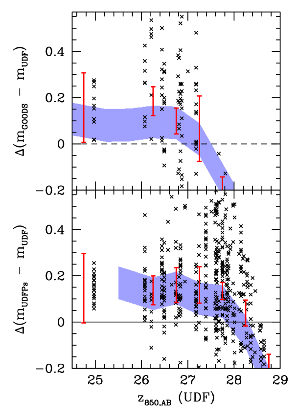
Figure 19.— Differences between the $z_{850,AB}$-band magnitudes measured for $i$-dropouts in the HUDF and those measured after degrading these data to the depths of our shallower fields and reselecting these objects (see Appendix C for a description of these simulations). The results of 10 different degradations of the HUDF to GOODS depth are shown (top). Twenty different degradations of the HUDF to HUDF-Ps depth are included in the bottom panel (10 for HUDFP1 and 10 for HUDFP2). The red vertical bars (positioned at half-magnitude intervals) denote the 68% confidence intervals on the mean magnitude shift (clipped to exclude large $>0.45$ mag deviations). The blue shaded region shows the shifts obtained when repeating these experiments on several simulated fields used to extract our transfer functions (Appendix D3). The width of the shaded region ($\pm 0.07$ mag) provides suggested error bars on the derived shifts due to systematic (different deblending effects with nearby objects) and random errors (limited number of input templates in the simulations). Although there is some indication, particularly in the top panel, that the derived shifts from the observations (red error bars) are larger than those obtained from the simulations (blue shaded region), this may simply be an artefact of the objects we use to make these estimates (three objects from the HUDF were used to derive the mean shifts for the brightest two magnitude intervals). The shifts are similar enough to give us confidence in using the simulations to determine our transfer functions.

D.3. Transfer Functions

The completeness and flux corrections detailed in Appendix D1 and D2 can be more properly implemented using transfer functions. Transfer functions take surface densities observed at one depth and convert them to their equivalent densities if measured at another. In this formulation, incompleteness is incorporated as a decrease in the surface density from the input to output stage. Magnitude biases are included by effecting a shift from one magnitude interval to another.

Ideally, we would determine the transfer functions in the same way as we estimate the completeness and flux biases in the previous sections (e.g., by performing degradation experiments on the real data). Unfortunately, the available data are simply not sufficient to adequately determine these functions. Without a large number of input objects, the computed transfer functions would be overly dependent on the position of particular objects within the different magnitude bins (and their morphologies), compromising the overall accuracy of the simulations. This is particularly true at bright magnitudes ($z_{850,AB}\lesssim 26$) where there is only one object in our deeper fields.

As such, it appeared that our best option was simply to rely on simulations–again using our cloning software to generate the mock fields. The inputs to the simulations consisted of $B$-dropout samples from both the HUDF-Ps (Bouwens et al. 2004b) and the HUDF (Bouwens et al. 2004b). Our use of $z\sim 3.8$ $B$-dropout samples was motivated by the much higher surface brightness sensitivites available for $B$-dropouts than for $i$-dropouts in the same data [due to $(1+z)^{4}$ cosmic surface brightness dimming]. Moreover, objects from these samples should be fairly similar to the $i$-dropout sample in both size and morphology, minimizing the importance of different assumptions regarding their evolution over cosmic time ($\sim$700 Myr). Objects were projected over the range $z\sim 5.2-7.0$ in accordance with their volume density and then added to the artificial HUDF frames. Object sizes were scaled as $(1+z)^{-1.1}$ (for fixed luminosity) to match the observed scalings (§3.7).

Our transfer functions were calculated by degrading the above simulations and then comparing the magnitudes of objects selected on the original frames (at HUDF depths) with those selected on the degraded frames. The transfer functions are initially binned on 0.1 mag scales to form familiar two-dimensional matrices, and then smoothed along the diagonals (to improve the statistics while preserving flux biases). The smoothing length is set so that at least 30 different objects from our simulated images contribute to each element in this matrix (this is equivalent to a smoothing length of $\Delta m\sim 0.5$ at $z_{850,AB}<25.5$, but $\Delta m\sim 0.1$ at $z_{850,AB}\gtrsim 26.5$). After smoothing, the results are rebinned on 0.5 mag intervals to match the binning for the number counts (Figure 5). A tabulation of our two transfer functions is provided in Tables D5 and D6. They are expressed in such a way that one can use matrix multiplication procedures to go from surface densities selected in HUDF-type data to the equivalent surface densities measured in the shallower data. Note that since object blending is not properly included in these simulations (the surface density of objects is comparably low), we corrected our transfer functions upwards to account for the greater incompleteness in the HUDF due to object blending (see Appendix D1).

Table 19Transfer Function to take the surface densities measured at HUDF depths to their equivalent surface densities at GOODS and HUDF-Ps depths (Appendix D3).

	HUDF
GOODS	$z_{850}$ Band (mag)
$z_{850}$ band	24.25	24.75	25.25	25.75	26.25	26.75	27.25	27.75	28.25	28.75	29.25
24.25	0.776	0.011	0.000	0.000	0.000	0.000	0.000	0.000	0.000	0.000	0.000
24.75	0.326	0.817	0.008	0.000	0.000	0.000	0.000	0.000	0.000	0.000	0.000
25.25	0.000	0.255	0.711	0.018	0.000	0.000	0.000	0.000	0.000	0.000	0.000
25.75	0.000	0.000	0.279	0.658	0.024	0.000	0.000	0.000	0.000	0.000	0.000
26.25	0.000	0.000	0.017	0.256	0.600	0.041	0.000	0.000	0.000	0.000	0.000
26.75	0.000	0.000	0.002	0.018	0.219	0.415	0.044	0.000	0.000	0.000	0.000
27.25	0.000	0.000	0.000	0.002	0.030	0.229	0.241	0.028	0.000	0.000	0.000
27.75	0.000	0.000	0.000	0.000	0.002	0.014	0.073	0.030	0.001	0.000	0.000
28.25	0.000	0.000	0.000	0.000	0.000	0.000	0.000	0.000	0.000	0.000	0.000
28.75	0.000	0.000	0.000	0.000	0.000	0.000	0.000	0.000	0.000	0.000	0.000
29.25	0.000	0.000	0.000	0.000	0.000	0.000	0.000	0.000	0.000	0.000	0.000

Table 20Transfer Function to take the surface densities measured at HUDF depths to their equivalent surface densities at HUDF-Ps depths (Appendix D3).

	HUDF
HUDF-Ps	$z_{850}$ Band (mag)
$z_{850}$ band	24.25	24.75	25.25	25.75	26.25	26.75	27.25	27.75	28.25	28.75	29.25
24.25	0.899	0.006	0.000	0.000	0.000	0.000	0.000	0.000	0.000	0.000	0.000
24.75	0.180	0.922	0.008	0.000	0.000	0.000	0.000	0.000	0.000	0.000	0.000
25.25	0.000	0.153	0.862	0.013	0.000	0.000	0.000	0.000	0.000	0.000	0.000
25.75	0.000	0.000	0.202	0.800	0.013	0.000	0.000	0.000	0.000	0.000	0.000
26.25	0.000	0.000	0.000	0.248	0.755	0.022	0.000	0.000	0.000	0.000	0.000
26.75	0.000	0.000	0.000	0.001	0.272	0.644	0.035	0.000	0.000	0.000	0.000
27.25	0.000	0.000	0.000	0.000	0.016	0.277	0.633	0.040	0.001	0.000	0.000
27.75	0.000	0.000	0.000	0.000	0.003	0.026	0.247	0.408	0.055	0.001	0.001
28.25	0.000	0.000	0.000	0.000	0.000	0.005	0.018	0.208	0.223	0.028	0.001
28.75	0.000	0.000	0.000	0.000	0.000	0.001	0.000	0.009	0.021	0.014	0.000
29.25	0.000	0.000	0.000	0.000	0.000	0.000	0.000	0.000	0.000	0.000	0.000

It is possible to obtain a useful check on the results obtained from these simulated fields by estimating the completeness levels and flux biases on these same fields. Our estimates of these quantities were computed in a way very similar to how they were computed on the actual data (i.e., Appendix D1 and D2) to ensure consistency. The results are shown in the “SIM” columns of Table D3 and in Figure D2 (blue shaded regions) and appear to be in broad agreement with those obtained from our degradation experiments. This provides us with confidence in the transfer functions we determine from the simulations.

D.4. Contamination Corrections

In principle, the availability of $B_{435}$ and $V_{606}$-band imaging provides an effective means of eliminating contaminants directly. Lower redshift interlopers are expected to be significantly brighter in the $B_{435}$ and $V_{606}$-bands than genuine high-redshift objects and therefore our requirement that objects be redder than 2.8 in $V_{606}-z_{850}$ (Figure A1, Appendix A) should prove to be an effective means of eliminating such objects. Unfortunately, near the magnitude limit of each field, only limited constraints can be set on the $V_{606}$-band fluxes and therefore it is difficult to effectively filter out all contaminants.

We can however estimate this contamination statistically, using the deeper optical and infrared data available for some of our fields. We break these contamination estimates into four different components: (1) contamination from intrinsically red objects, (2) contamination from photometric scatter, (3) contamination from low mass stars, and (4) contamination from spurious sources. Explicit effort is made to ensure that the contribution from each component is independent (and thus no contaminant is subtracted twice).

D.4.1 Contamination from Intrinsically Red Objects

A small fraction of low-redshift ($z\sim 1-3$) galaxies have colors that are red enough to satisfy our $(i_{775}-z_{850})_{AB}>1.3$ selection. Since such objects have very different optical-infrared colors from bona-fide $z\sim 6$ objects (Figures 3 and D3), we can use the deep infrared data available to make an estimate of the approximate contamination rate. We already provided a preliminary estimate of this contamination rate from the HUDF in §3.2, but we can obtain a much better estimate of this contamination rate at bright magnitudes ($25<z_{850,AB}<27$) using the ISAAC data available over the CDF-S GOODS field. Similar to the procedures outlined at the beginning of §3, $z_{850}-J$ and $z_{850}-K_{s}$ colors for $i$-dropouts in CDF-South GOODS were measured by smoothing the $z_{850}$-band data to the same PSF as in the infrared images and measuring the flux in an aperture whose diameter was 2 times the FWHM of the object. Compiling galaxies from the entire 131 arcmin² CDF-S ISAAC mosaic, candidate low-$z$ interlopers were identified with the criteria: $(i_{775}-z_{850})_{AB}>1.3,(z_{850}-K_{s})_{AB}>1.6$. Only two such objects were found (Figure D3): one at $z_{850,AB}\sim 25.4$ and one at $z_{850,AB}\sim 26.0$. The majority of objects with $i_{775}-z_{850}>1.3$ colors had $(z_{850}-K_{s})_{AB}$ colors bluer than 1.6. Over the interval $25.0<z_{850,AB}<26.0$, this works out to $18_{-9}^{+13}$% contamination rate from intrinsically red objects and over the interval $26.0<z_{850,AB}<27.0$, the contamination rate is $\lesssim 2$% ($1\sigma$). These results are combined with similar estimates from the HUDF IR data (§3.2) and summarized in Table D7.

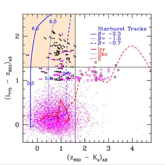
Figure 20.— The $(i_{775}-z_{850})_{AB}$/$(z_{850}-K_{s})_{AB}$ colors of objects in the CDF-S GOODS field (Appendix D4.1) with $z_{850,AB}<26.8$. Objects that are undetected ($<2\sigma$) in the $V_{606}$-band are shown in black while objects which are detected at the $2\sigma$ level are shown in magenta. Objects that made it into our low-redshift interloper selection [Table 2; $(i_{775}-z_{850})_{AB}>1$ and $(z_{850}-J)_{AB}>0.8$] are shown as enlarged open squares (see also Figure A1). Otherwise objects are shown as small filled circles. Color-color tracks of low-redshift templates and high-redshift starbursts with different reddenings are as in Figure 2. Arrows denote $2\sigma$ limits on the $(i_{775}-z_{850})_{AB}$ and $(z_{850}-K_{s})_{AB}$ colors. The solid horizontal line shows our $(i_{775}-z_{850})_{AB}$ cut for selecting $i$-dropouts while the solid vertical line shows our $(z_{850}-K_{s})_{AB}$ cut which serves to separate dropouts from intrinsically red objects (Figure A1). The majority ($\lesssim 2$%) of objects with $i_{775}-z_{850}>1.3$ colors had $(z_{850}-K_{s})_{AB}$ colors bluer than 1.6. This suggests that contamination from intrinsically red objects is very small ($\lesssim 2$%: Table D7).

Table 21The estimated number of intrinsic red contaminants using the CDF-S GOODS + HUDF data

	GOODS	HUDF
Magnitude Interval	(arcmin-2)	(arcmin-2)
$24.0<z_{850,AB}<25.0$	0.000 ($<43$%)	0.000 ($<43$%)
$25.0<z_{850,AB}<26.0$	0.014 ($18_{-9}^{+13}$%)	–
$26.0<z_{850,AB}<27.0$	0.000 ($<2$%)	0.000 ($<17$%)
$27.0<z_{850,AB}<28.0$	–	0.000 ($<6$%)
$28.0<z_{850,AB}<29.0$	–	0.767 ($10_{-5}^{+8}$%)
$29.0<z_{850,AB}<29.5$	–	–

D.4.2 Contamination from Photometric Scatter

Here we estimate the contamination rate from photometric scatter. As with our estimates of the completeness levels and flux biases, perhaps the most model-independent procedure is to use the results of our degradation experiments described earlier (Appendix C). Objects that are selected as $i$-dropouts can be compared with the original source catalogs available for the HUDF and HUDF-Ps fields and contaminants identified. The results of these simulations are compiled in Tables D8-D9 as a function of magnitude, and again this source of contamination is small ($\lesssim 10$%) and only of significance within $\approx 1$ mag of the faint-end limit.

In our shallower fields, contamination from photometric scatter can effectively be controlled for using degradations of the HUDF. However, the HUDF itself has no deeper field that can serve as a control (which is an issue faintward of $z_{850,AB}\sim 28.5$ where the HUDF $V_{606}$-band fluxes are no longer of sufficient S/N to filter out contaminants). Therefore, we needed an alternative procedure, and so we elected to model the faint objects in our catalog with the colors of intermediate magnitude $25.9<z_{850,AB}<27.4$ objects and then add photometric scatter. To ensure that the intermediate magnitude objects were really at low redshift, we required the objects to have $(i_{775}-z_{850})_{AB}$ colors bluer than 0.9 and $(V_{606}-z_{850})_{AB}$ colors bluer than 2.5. These criteria explicitly excluded objects that were close to qualifying as $i_{775}$-dropouts (see Figure D4). In performing the simulations, we iterated over all faint $z_{850,AB}>27.9$ objects in the HUDF (2908 objects), randomly picking an intermediate magnitude object and then perturbing this object’s photometry to match the S/N of the faint object we were iterating over. After repeating this scattering experiment on all faint objects in the HUDF in four separate trials, we found only one contaminant, or just 0.25 contaminant per 11 arcmin² field. This is a smaller fraction than what we found in our simulations of the HUDF-Ps and GOODS fields (Tables D8-D9) and may owe to the depth of the HUDF $i_{775}$-band imaging. In our other fields, the $i_{775}$-band depths only exceeded the $z_{850}$-band depths by $\sim$0.4 mag, but in the HUDF this difference is 0.7 mag. Also note that because at faint magnitudes almost all objects are blue $(i_{775}-z_{850})\lesssim 0.6$, $(V_{606}-z_{850})_{AB}<1.3$, most objects would still be quite significant detections in the bluer bands at the limits of the HUDF $i_{775}$-dropout probe ($z_{850,AB}\sim 29.5$).

Table 22The estimated number of contaminants in our GOODS and HUDF-Ps $i$-dropout samples resulting from photometric scatter.

	GOODS	HUDF-Ps
Magnitude Interval	(arcmin-2)	(arcmin-2)
$24.0<z_{850,AB}<24.5$	0.00	0.00
$24.5<z_{850,AB}<25.0$	0.00	0.00
$25.0<z_{850,AB}<25.5$	0.00	0.00
$25.5<z_{850,AB}<26.0$	0.00	0.00
$26.0<z_{850,AB}<26.5$	0.01	0.00
$26.5<z_{850,AB}<27.0$	0.01	0.00
$27.0<z_{850,AB}<27.5$	0.04	0.01
$27.5<z_{850,AB}<28.0$	0.01	0.18
$28.0<z_{850,AB}<28.5$	–	0.12
$28.5<z_{850,AB}<29.0$	–	0.08

Table 23The estimated number of contaminants in our GOODS $i$-dropout sample resulting from photometric scatter.

	GOODS
Magnitude Interval	(arcmin-2)
$24.0<z_{850,AB}<24.5$	0.00
$24.5<z_{850,AB}<25.0$	0.00
$25.0<z_{850,AB}<25.5$	0.00
$25.5<z_{850,AB}<26.0$	0.00
$26.0<z_{850,AB}<26.5$	0.02
$26.5<z_{850,AB}<27.0$	0.01
$27.0<z_{850,AB}<27.5$	0.01
$27.5<z_{850,AB}<28.0$	0.02

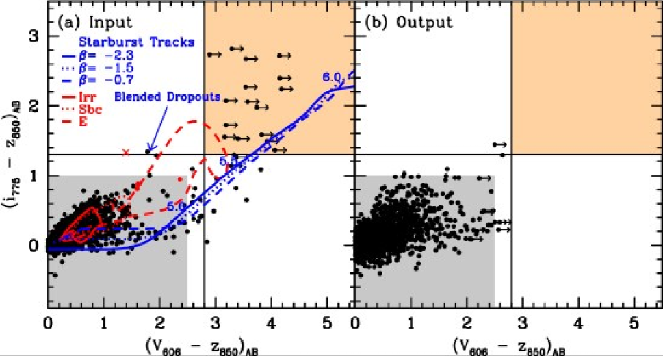
Figure 21.— (a) The intermediate magnitude photometric sample (gray shaded region in the bottom left-hand corner) used to estimate the susceptibility of our faint ($z_{850,AB}>27.9$) HUDF $i$-dropout sample to contamination from low-redshift interlopers due to photometric scatter. Shown are the $(i_{775}-z_{850})_{AB}/(V_{606}-z_{850})_{AB}$ colors of faint $25.9<z_{850,AB}<27.4$ objects from the HUDF (black circles). The horizontal and vertical lines show the $(i_{775}-z_{850})_{AB}$ and $(V_{606}-z_{850})_{AB}$ selection cuts used for selecting $i$-dropouts. Objects that are particularly red ($\gtrsim 0.7$) in $(z_{850}-J_{110})_{AB}$ and therefore likely low-redshift early-types are shown as red circles. Arrorws indicate $2\sigma$ lower limits. The color-color tracks for low-redshift interlopers are also included (in red) along with the position of high-redshift starbursts with various amounts of reddening (in blue). Objects in the top right-hand corner (orange shaded region) are $i$-dropouts, and objects in the lower right-hand corner are objects that are likely just below our redshift cut. The position of two $i$-dropouts that is partially blended with foreground objects are indicated by the blue arrow (Table D4) while the position of one point-like star is indicated by the red cross. (b) The $(i_{775}-z_{850})_{AB}/(V_{606}-z_{850})_{AB}$ colors for objects from the HUDF input sample (bottom left-hand corner with gray shading) scattered to match the photometric errors of faint ($z_{850,AB}>27.9$) objects in the HUDF. The output of the simulations indicates that contamination from photometric scatter at faint magnitudes is negligible ($<1$ object) (see Appendix D4.2).

D.4.3 Contamination from Low-mass Stars

Low mass stars have similar $(i_{775}-z_{850})_{AB}$ colors to $z\sim 6$ objects, and therefore can act as contaminants to our samples. Fortunately, this has not proven to be an important concern, mostly because the majority of $i$-dropouts ($\gtrsim 90\%$) are clearly resolved at ACS resolution (0.10^′′ FWHM) and therefore it is possible to distinguish these objects (which have typical half-light radii of $\sim 0.1-0.2$^′′) from stellar contaminants. We have found that the SExtractor stellarity parameter works particularly well in this regard, especially for sources with significant ($>10\sigma$) detections in the $z_{850}$ band. Such S/Ns are achieved at $z_{850,AB}\lesssim 26.8$ for the GOODS fields, $z_{850,AB}\lesssim 27.5$ for the HUDF-Ps, and $z_{850,AB}\lesssim 28.4$ for the HUDF.

Unfortunately, beyond these limits, the SExtractor stellarity parameter no longer gives reliable results – making it difficult to use this statistic to identify and remove stellar sources. So, the question becomes: how shall we deal with contamination from stars at such magnitudes? We think the best approach is a statistical one: (1) determine the fraction of low-mass stars in $i$-dropout samples as a function of magnitude using the deeper ACS data and then (2) apply that contamination fraction to the shallower data. An estimate of this contamination fraction can be obtained by examining the data at all three depths and plotting the fraction of point-like objects as a function of the $z_{850}$-band magnitude in all three fields. As is clear in Figure D5, there is a monotonic decrease in the fraction of these objects with magnitude, from $\sim 80-100$% at bright magnitudes ($z_{850,AB}\sim 23-25$) to a mere $\sim$1-2% at fainter magnitudes ($z_{850,AB}\sim 26-27$).

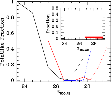
Figure 22.— Fraction of $i$-dropout candidates that are point-like (SExtractor stellarity $>$0.75, where 0 is an extended object and 1 is a point source) and thus likely stellar contaminants vs. $z_{850}$-band magnitude. The main panel shows the observed fraction in the HUDF (red lines), HUDF-Ps (blue lines), and GOODS fields (black lines). The red and blue lines are offset slightly from zero for clarity. The lines become dotted at the point where the S/N is too low to discriminate between extended and point-like objects. Inset; The assumed fraction of stellar contaminants (the shaded red region shows the assumed $1\sigma$ uncertainties). Stellar contaminants are rejected using the measured stellarities brightward of $z_{850,AB}$ equal to 28.4, 27.5, and 26.8, for the HUDF, HUDF-Ps, and GOODS fields, respectively. Faintward of this, no such attempt is made and a contamination fraction is assumed, based on an extrapolation from bright magnitudes (see Appendix D4.3 for more details).

Connecting the surveys up and extrapolating the trends beyond $z_{850,AB}\sim 28.4$, we can arrive at an approximate contamination fraction as a function of magnitude (Figure D5, inset). By multiplying these fractions by the observed surface densities (Table 11), the contamination rate from low mass stars can be derived (see Ryan et al. 2005 for independent estimates).

D.4.4 Contamination from Spurious Sources

In principle, our samples were also sensitive to contamination from spurious objects resulting from noise spikes or other non-Gaussian features. If present, such spurious sources would easily qualify as dropouts given the unlikelihood that similar spikes would occur in the other passbands. Therefore, analogous to the simulations described in B06a, Dickinson et al. (2004), and Yan & Windhorst (2004b), we repeated our selection procedure on the negative images, and similar to the results in B06a and Yan & Windhorst (2004b), no objects were found in our data sets at all three depths. Therefore, it seems unlikely that spurious objects represent a significant source of contamination for our samples ($\lesssim 1$%).

D.4.5 Summary

Table D10 shows the sum of all three sources of contamination for the samples considered here (spurious sources do not appear to be a concern). Totaling up these results for all three samples and all magnitude intervals, we can arrive at an approximate contamination rate for our cumulative sample. This result is $\lesssim 8$% (i.e., $\gtrsim 92$% of $i$-dropouts are at $z\sim 6$).

Table 24Total Contamination Rate (Intrinsically Red + Photometric Scatter + Stars).

	Field
	GOODS	HUDF-Ps	HUDF
Magnitude Range	(arcmin-2)	(arcmin-2)	(arcmin-2)
$24.0<z_{850}<24.5$	0.000	0.000	0.000
$24.5<z_{850}<25.0$	0.000	0.000	0.000
$25.0<z_{850}<25.5$	0.003	0.000	0.000
$25.5<z_{850}<26.0$	0.010	0.000	0.000
$26.0<z_{850}<26.5$	0.015	0.000	0.000
$26.5<z_{850}<27.0$	0.010	0.000	0.000
$27.0<z_{850}<27.5$	0.022	0.009	0.000
$27.5<z_{850}<28.0$	0.016	0.198	0.000
$28.0<z_{850}<28.5$	–	0.310	0.147
$28.5<z_{850}<29.0$	–	0.094	0.467
$29.0<z_{850}<29.5$	–	–	0.177

Appendix E Uncertainties in the LF due to Field-to-Field Variations

In deriving the rest-frame continuum $UV$ luminosity function at $z\sim 6$, we make use of $i$-dropouts from three different fields. One possibly significant concern is that since the surface density of $i$-dropouts can show significant differences in normalization from one field to another (we expect $\sim$35% rms for a 11.3 arcmin² ACS field: §3.6), these differences may have an effect on our derived LF. To quantify the size of this effect, we ran a series of Monte-Carlo simulations. Using the normalization $\phi^{*}=0.00202\,\textrm{Mpc}^{-3}$, faint-end slope $\alpha=-1.73$ from our best-fit LF (§5), and an ensemble of different characteristic luminosities $M_{1350,AB}^{*}$ (i.e., $-19.75$, $-19.85$, $-19.95$, …, $-20.65$) scattered around our preferred value of $M_{1350,AB}^{*}=-20.25$ (§5), we generated number count predictions for each of our fields (i.e., the HUDF, the HUDF-Ps, and the GOODS fields). Our computed counts included the relevant selection and measurement biases as shown in Tables D5-D6 and Figure 8. We varied the normalization on our counts for our deepest two fields (i.e., the HUDF and HUDF-Ps) by 30% rms (the approximate uncertainties on the relative normalization of our different fields), combined the counts from all our fields (§3.8), and then fit them to a Schechter function (§5). Repeating this experiment 100 times using different normalizations for our three fields, we derived rms errors on our three Schechter parameters that result from the uncertain normalizations. The rms errors on $\alpha$ were consistently $\sim 0.20$ for all input values of $M_{1350}^{*}$, while the rms errors on $M_{1350}^{*}$ and $\phi^{*}$ increased from 0.10 and 0.00041, respectively, for fainter values of $M_{1350}^{*}$ (i.e., $-19.65$) to 0.17 and 0.00065, respectively, for brighter values of $M_{1350}^{*}$ (i.e., $-20.65$). This suggests that it is currently not possible to determine the normalization of the luminosity function $\phi^{*}$ to better than 30% and the faint-end slope $\alpha$ to better than 0.2.

References

- Adelberger & Steidel (2000) Adelberger, K. L. & Steidel, C. C. 2000, ApJ, 544, 218
- Ajiki et al. (2003) Ajiki, M., et al. 2003, AJ, 126, 2091
- Arnouts et al. (2001) Arnouts, S., et al. 2001, A&A, 379, 740
- (4) Arnouts, S., et al. 2005, ApJ, 619, L43
- Bardeen, Bond, Kaiser, & Szalay (1986) Bardeen, J. M., Bond, J. R., Kaiser, N., & Szalay, A. S. 1986, ApJ, 304, 15
- Barkana & Loeb (1999) Barkana, R. & Loeb, A. 1999, ApJ, 523, 54
- Becker et al. (2001) Becker, R. H. et al. 2001, AJ, 122, 2850
- Beckwith et al. (2006) Beckwith, S. V. W., et al. 2006, AJ, 132, 1729
- Bertin and Arnouts (1996) Bertin, E. and Arnouts, S. 1996, A&AS, 117, 393
- Binney (2004) Binney, J. 2004, MNRAS, 347, 1093
- (11) Birnboim, Y. & Dekel, A. 2003, MNRAS, 345, 349
- Blakeslee et al. (2003) Blakeslee, J. P., Anderson, K. R., Meurer, G. R., Benítez, N., & Magee, D. 2003a, ASP Conf. Ser. 295: Astronomical Data Analysis Software and Systems XII, 12, 257
- Blakeslee et al. (2004) Blakeslee, J. P., et al. 2004, ApJ, 602, L9
- Bouwens, Broadhurst and Silk (1998) Bouwens, R., Broadhurst, T. and Silk, J. 1998a, ApJ, 506, 557
- Bouwens, Broadhurst and Silk (1998) Bouwens, R., Broadhurst, T. and Silk, J. 1998b, ApJ, 506, 579.
- Bouwens, Broadhurst, & Illingworth (2003) Bouwens, R., Broadhurst, T., & Illingworth, G. 2003a, ApJ, 593, 640
- Bouwens et al. (2003) Bouwens, R. J. et al. 2003b, ApJ, 595, 589
- Bouwens et al. (2004) Bouwens, R. J., et al. 2004a, ApJ, 606, L25
- Bouwens et al. (2004) Bouwens, R. J., Illingworth, G.D., Blakeslee, J.P., Broadhurst, T.J., & Franx, M. 2004b, ApJ, 611, L1
- Bouwens et al. (2004) Bouwens, R. J., et al. 2004c, ApJ, 616, L79
- Bouwens et al. (2005) Bouwens, R. J., Illingworth, G.D., Thompson, R.I., & Franx, M. 2005, ApJ, 624, L5
- Bouwens et al. (2006) Bouwens, R. J., Illingworth, G.D., Broadhurst, T.J., Meurer, G.R., Blakeslee, J.P., Franx, M., & Ford, H.C. 2006a, ApJ, submitted (B06a)
- Bouwens et al. (2006) Bouwens, R. J., Broadhurst, T.J., Illingworth, G.D., Meurer, G.R., Blakeslee, J.P., Franx, M., & Ford, H.C. 2006b, ApJ, submitted (B06b)
- Bunker, Stanway, Ellis, & McMahon (2004) Bunker, A. J., Stanway, E. R., Ellis, R. S., & McMahon, R. G. 2004, MNRAS, 355, 374
- Cimatti et al. (2002) Cimatti, A., et al. 2002, A&A, 381, L68
- Coe et al. (2006) Coe, D., Benítez, N., Sánchez, S.F., Jee, M., Bouwens, R., Ford, H. 2006, AJ, in press, astro-ph/0605262
- Coleman, Wu, & Weedman (1980) Coleman, G. D., Wu, C. -., & Weedman, D. W. 1980, ApJS, 43, 393
- Cooray (2005) Cooray, A. 2005, MNRAS, 364, 303
- Croton et al. (2005) Croton, D., et al. 2005, MNRAS, 365, 11
- Daddi et al. (2003) Daddi, E., et al. 2003, ApJ, 588, 50
- Deharveng et al. (2001) Deharveng, J.-M., Buat, V., Le Brun, V., Milliard, B., Kunth, D., Shull, J. M., & Gry, C. 2001, A&A, 375, 805
- (32) de Jong, R.S., et al. 2006, The 2005 HST Calibration Workshop, 121.
- Dickinson et al. (2004) Dickinson, M. et al. 2004, ApJ, 600, L99
- Di Matteo et al. (2005) Di Matteo, T., Springel, V., & Hernquist, L. 2005, Nature, 433, 604
- (35) Dow-Hygelund, C. et al. 2006, submitted
- Fan et al. (2002) Fan, X., Narayanan, V. K., Strauss, M. A., White, R. L., Becker, R. H., Pentericci, L., & Rix, H. 2002, AJ, 123, 1247
- Ferguson et al. (2004) Ferguson, H. C. et al. 2004, ApJ, 600, L107
- Fernández-Soto, Lanzetta, & Chen (2003) Fernández-Soto, A., Lanzetta, K. M., & Chen, H.-W. 2003, MNRAS, 342, 1215
- (39) Gabasch, A., et al. 2004, A&A, 421, 41.
- Giallongo, Cristiani, D’Odorico, & Fontana (2002) Giallongo, E., Cristiani, S., D’Odorico, S., & Fontana, A. 2002, ApJ, 568, L9
- Geballe et al. (2002) Geballe, T. R., et al. 2002, ApJ, 564, 466
- Giavalisco et al. (2004) Giavalisco, M., et al. 2004a, ApJ, 600, L93
- Giavalisco et al. (2004) Giavalisco, M., et al. 2004b, ApJ, 600, L103
- Gnedin & Ostriker (1997) Gnedin, N. Y. & Ostriker, J. P. 1997, ApJ, 486, 581
- Granato et al. (2004) Granato, G. L., De Zotti, G., Silva, L., Bressan, A., & Danese, L. 2004, ApJ, 600, 580
- Hu et al. (2004) Hu, E. M., Cowie, L. L., Capak, P., McMahon, R. G., Hayashino, T., & Komiyama, Y. 2004, AJ, 127, 563
- Hurwitz, Jelinsky, & Dixon (1997) Hurwitz, M., Jelinsky, P., & Dixon, W. V. D. 1997, ApJ, 481, L31
- Inoue et al. (2005) Inoue, A. K., Iwata, I., Deharveng, J.-M., Buat, V., & Burgarella, D. 2005, A&A, 435, 471
- Iwata et al. (2003) Iwata, I., Ohta, K., Tamura, N., Ando, M., Wada, S., Watanabe, C., Akiyama, M., & Aoki, K. 2003, PASJ, 55, 415
- Knapp et al. (2004) Knapp, G. R., et al. 2004, AJ, 127, 3553
- Kneib, Ellis, Santos, & Richard (2004) Kneib, J., Ellis, R. S., Santos, M. R., & Richard, J. 2004, ApJ, 607, 697
- Kodaira et al. (2003) Kodaira, K., et al. 2003, PASJ, 55, L17
- Kron (1980) Kron, R. G. 1980, ApJS, 43, 305
- Leggett et al. (2002) Leggett, S. K., et al. 2002, ApJ, 564, 452
- Lehmer et al. (2005) Lehmer, B. D., et al. 2005, AJ, 129, 1
- Lehnert & Bremer (2003) Lehnert, M. D. & Bremer, M. 2003, ApJ, 593, 630
- Leitherer, Ferguson, Heckman, & Lowenthal (1995) Leitherer, C., Ferguson, H. C., Heckman, T. M., & Lowenthal, J. D. 1995, ApJ, 454, L19
- Leitherer et al. (1999) Leitherer, C., et al. 1999, ApJS, 123, 3
- Madau et al. (1998) Madau, P., Pozzetti, L. & Dickinson, M. 1998, ApJ, 498, 106
- Madau, Haardt, & Rees (1999) Madau, P., Haardt, F., & Rees, M. J. 1999, ApJ, 514, 648
- Malkan, Webb, & Konopacky (2003) Malkan, M., Webb, W., & Konopacky, Q. 2003, ApJ, 598, 878
- Malhotra et al. (2005) Malhotra, S., et al. 2005, ApJ, 626, 666
- Martin et al. (2005) Martin, D. C., et al. 2005, ApJ, 619, L59
- Mo & White (1996) Mo, H. J., & White, S. D. M. 1996, MNRAS, 282, 347
- Nagao et al. (2004) Nagao, T., et al. 2004, ApJ, 613, L9
- Night et al. (2006) Night, C., Nagamine, K., Springel, V., & Hernquist, L. 2006, MNRAS, 366, 705
- Ouchi et al. (2004) Ouchi, M., et al. 2004, ApJ, 611, 660
- Pirzkal et al. (2004) Pirzkal, N., et al. 2004, ApJS, 154, 501
- Pirzkal et al. (2005) Pirzkal, N., et al. 2005, ApJ, 622, 319
- Press & Schechter (1974) Press, W. H. & Schechter, P. 1974, ApJ, 187, 425
- Reddy & Steidel (2004) Reddy, N. A., & Steidel, C. C. 2004, ApJ, 603, L13
- Ryan et al. (2005) Ryan, R. E., Jr., Hathi, N. P., Cohen, S. H., & Windhorst, R. A. 2005, ApJ, 631, L159
- Sandage, Tammann, & Yahil (1979) Sandage, A., Tammann, G. A., & Yahil, A. 1979, ApJ, 232, 352
- Sawicki & Thompson (2005) Sawicki, M., & Thompson, D. 2005, ApJ, 635, 100
- Scannapieco & Oh (2004) Scannapieco, E., & Oh, S. P. 2004, ApJ, 608, 62
- Scannapieco et al. (2005) Scannapieco, E., Silk, J., & Bouwens, R. 2005, ApJ, 635, L13
- Schaerer & Pelló (2005) Schaerer, D., & Pelló, R. 2005, MNRAS, 362, 1054
- Schechter (1976) Schechter, P. 1976, ApJ, 203, 297
- Schiminovich et al. (2005) Schiminovich, D., et al. 2005, ApJ, 619, L47
- Schlegel, Finkbeiner, & Davis (1998) Schlegel, D. J., Finkbeiner, D. P., & Davis, M. 1998, ApJ, 500, 525
- Sheth & Tormen (1999) Sheth, R. K. & Tormen, G. 1999, MNRAS, 308, 119
- Shimasaku et al. (2005) Shimasaku, K., Ouchi, M., Furusawa, H., Yoshida, M., Kashikawa, N., & Okamura, S. 2005, PASJ, 57, 447
- Sirianni et al. (2005) Sirianni, M., et al. 2005, PASP, 117, 1049
- Skrutskie et al. (1997) Skrutskie, M. F., et al. 1997, ASSL Vol. 210: The Impact of Large Scale Near-IR Sky Surveys, 25
- Somerville et al. (2004) Somerville, R. S., Lee, K., Ferguson, H. C., Gardner, J. P., Moustakas, L. A., & Giavalisco, M. 2004, ApJ, 600, L171
- Spergel et al. (2003) Spergel, D. N., et al. 2003, ApJS, 148, 175
- Stanway, Bunker, & McMahon (2003) Stanway, E. R., Bunker, A. J., & McMahon, R. G. 2003, MNRAS, 342, 439
- Stanway et al. (2004) Stanway, E. R., et al. 2004a, ApJ, 604, L13
- Stanway et al. (2004) Stanway, E. R., Bunker, A. J., McMahon, R. G., Ellis, R. S., Treu, T., & McCarthy, P. J. 2004b, ApJ, 607, 704
- Stanway et al. (2005) Stanway, E. R., McMahon, R. G., & Bunker, A. J. 2005, MNRAS, 359, 1184
- Steidel et al. (1999) Steidel, C. C., Adelberger, K. L., Giavalisco, M., Dickinson, M. and Pettini, M. 1999, ApJ, 519, 1
- Steidel, Pettini, & Adelberger (2001) Steidel, C. C., Pettini, M., & Adelberger, K. L. 2001, ApJ, 546, 665
- Stiavelli, Fall, & Panagia (2004) Stiavelli, M., Fall, S. M., & Panagia, N. 2004a, ApJ, 600, 508
- Stiavelli, Fall, & Panagia (2004) Stiavelli, M., Fall, S. M., & Panagia, N. 2004b, ApJ, 610, L1
- Thompson et al. (2005) Thompson, R. I., et al. 2005, AJ, 130, 1
- Trimble & Aschwanden (2005) Trimble, V., & Aschwanden, M. 2005, PASP, 117, 311
- Wang & Heckman (1996) Wang, B., & Heckman, T. M. 1996, ApJ, 457, 645
- White, Becker, Fan, & Strauss (2003) White, R. L., Becker, R. H., Fan, X., & Strauss, M. A. 2003, AJ, 126, 1
- Yan, Windhorst, & Cohen (2003) Yan, H., Windhorst, R. A., & Cohen, S. H. 2003, ApJ, 585, L93
- Yan & Windhorst (2004) Yan, H. & Windhorst, R. A. 2004a, ApJ, 600, L1
- Yan & Windhorst (2004) Yan, H. & Windhorst, R. A. 2004b, ApJ, 612, L93
- Yan et al. (2005) Yan, H., et al. 2005, ApJ, 634, 109