Multifrequency VLBA Monitoring of 3C 273 during the INTEGRAL Campaign in 2003

In this first of a series of papers describing polarimetric multifrequency Very Long Baseline Array (VLBA) monitoring of 3C 273 during a simultaneous campaign with the INTEGRAL $\gamma$-ray satellite in 2003, we present 5 Stokes I images and source models at 7 mm. We show that a part of the inner jet (1–2 milliarcseconds from the core) is resolved in a direction transverse to the flow, and we analyse the kinematics of the jet within the first 10 mas. Based on the VLBA data and simultaneous single-dish flux density monitoring, we determine an accurate value for the Doppler factor of the parsec scale jet, and using this value with observed proper motions, we calculate the Lorentz factors and the viewing angles for the emission components in the jet. Our data indicates a significant velocity gradient across the jet with the components travelling near the southern edge being faster than the components with more northern path. We discuss our observations in the light of jet precession model and growing plasma instabilities.

1 Introduction

Although vigorously investigated for over forty years, the physics of active galactic nuclei (AGN) have proved to be far from easily understandable. A set of basic facts about the nature of the central engine being a supermassive black hole and the gravitational accretion process as the primary energy source have been established beyond reasonable doubt, but the details of the picture do not quite fit. The intricate physics of AGN is made difficult by the complex interplay between several emission mechanism working simultaneously. For example, blazars, the class unifying flat-spectrum radio-loud quasars and BL Lac objects, contains sources that show significant radiation throughout the whole electromagnetic spectrum from radio to TeV $\gamma$-rays. The different emission mechanisms in AGNs include e.g. non-thermal synchrotron radiation from a relativistic jet, thermal emission from dust, optical-ultraviolet emission from the accretion disk, Comptonized hard X-rays from the accretion disk corona and $\gamma$-rays produced by inverse Compton scattering in the jet. Therefore, observing campaigns monitoring the sources simultaneously at as many wavelengths as possible are essential in studying AGNs.

Since the relativistic jet plays a crucial role in the objects belonging to the blazar class of AGNs, Very Long Baseline Interferometry (VLBI) observations imaging the parsec scale jet are an important addition to campaigns concentrating on this class. In particular, combined multifrequency VLBI monitoring and $\gamma$-ray measurements with satellite observatories may provide a solution to the question of the origin of the large amount of energy emitted in $\gamma$-rays by some blazars. By studying time lags between $\gamma$-ray flares and ejections of superluminal components into the VLBI jet, we should be able to establish whether the high energy emission comes from a region close to the central engine or whether it instead originates in the radio core or in the relativistic shocks – parsecs away from the black hole. In addition, multifrequency VLBI data yields spectra of the radio core and superluminal knots, which can be used to calculate the anticipated amount of the high energy emission due to the synchrotron self-Compton (SSC) process if an accurate value of the jet Doppler factor is known. Predicted SSC-flux can be directly compared with simultaneous hard X-ray and $\gamma$-ray observations.

Due to its proximity, 3C 273 (z=0.158; Schmidt sch63 (1963)) – the brightest quasar on the celestial sphere – is one of the most studied AGNs (see Courvoisier cou98 (1998) for a comprehensive review). Because 3C 273 exhibits all aspects of nuclear activity including a jet, a blue bump, superluminal motion, strong $\gamma$-ray emission and variability at all wavelengths, it was chosen as the target of an INTEGRAL campaign, where radiation above 1 keV was monitored in order to study the different high energy emission components (Courvoisier et al. cou03 (2003)). INTEGRAL observed 3C 273 in January, June-July 2003, and January 2004 and the campaign was supported by ground based monitoring at lower frequencies carried out at several different observatories (Courvoisier et al. cou04 (2004)). This article is the first in a series of papers describing a multifrequency polarimetric VLBI monitoring of 3C 273 using the Very Long Baseline Array (VLBA) in conjunction with the INTEGRAL campaign during 2003. The amount of data produced by such a VLBI campaign using six frequencies is huge. In order to divide the large volume of the gathered information into manageable chunks, we will treat the different aspects of the data (i.e. kinematics, spectra and polarisation) in different papers, and in the end we will attempt to draw a self-consistent picture taking into account the whole data set.

In the current paper we construct a template for the later analysis of the component spectra and polarisation, and for the comparison of the VLBI data with the INTEGRAL measurements. Since kinematics is important in all subsequent analyses, we start by studying the component motion in the jet within 10 mas from the radio core. The emphasis is on the components located close to the core ($\lesssim 2$ mas), since they are the most relevant for the combined analysis of the VLBI and INTEGRAL data. We use the 43 GHz data for the kinematical study, since they provide the best angular resolution with a good signal-to-noise ratio (SNR). The other frequencies are not discussed in this paper, since the positional errors at all other frequencies are significantly larger for the components we are interested in (i.e. those located near the core). Also, a kinematical analysis that takes into account multiple frequencies in a consistent way is very complicated using contemporary model fitting methods. However, the other frequencies are not ignored either; instead, we will check the compatibility of this paper’s results with the multifrequency data presented in the forthcoming papers treating the spectral information. In Paper II (Savolainen et al. in preparation) we will discuss the method to obtain the spectra of individual knots in the parsec scale jet, and present the spectra from the February 2003 observation. We will calculate the anticipated amount of SSC-radiation, and compare this with the quasi-simultaneous INTEGRAL data. In Papers III and IV, spectral evolution and polarisation properties of the superluminal components over the monitoring period will be presented. Paper V combines all the obtained information, to interpret it in a self-consistent way.

Throughout the paper, we use a contemporary cosmology with the following parameters: $H_{0}$ = 71 km s^-1 Mpc^-1, $\Omega_{M}$ = 0.27 and $\Omega_{\Lambda}$ = 0.73. For the spectral index, we use the positive convention: $S_{\nu}\propto\nu^{+\alpha}$.

2 Observations and data reduction

We observed 3C 273 with the National Radio Astronomy Observatory’s Very Long Baseline Array at five epochs in 2003 (February 28th, May 11th, July 2nd, September 7th and November 23rd) for nine hours at each epoch, using six different frequencies (5, 8.4, 15, 22, 43 and 86 GHz). The observations were carried out in the dual-polarisation mode enabling us also to study the linear polarisation of the source. However, we do not discuss the polarisation data here; it will be published in Paper IV (Savolainen et al. in preparation). At the first two epochs, 3C 279 was observed as a polarisation calibrator and as a flux calibrator. At the three later epochs, we added two more EVPA calibrators to the program: OJ 287 and 1611+343.

The data were calibrated at Tuorla Observatory using NRAO’s Astronomical Image Processing System (AIPS; Bridle & Greisen bri94 (1994)) and the Caltech Difmap package (Shepherd she97 (1997)) was used for imaging. Standard procedures of calibration, imaging and self-calibration were employed, and final images were produced with the Perl library FITSPlot.

Accuracy of a priori flux scaling was checked by comparing extrapolated zero baseline flux densities of a compact calibrator source, 3C 279, to near-simultaneous observations from VLA polarisation monitoring program (Taylor & Myers tay00 (2000)) and from Metsähovi Radio Observatory’s quasar monitoring program (Teräsranta et al. ter04 (2004)). The comparison shows that the a priori amplitude calibration of our data at 43 GHz is accurate to $\sim 5$%, which is better than the often quoted nominal value of 10%. A detailed discussion of the amplitude calibration and setting of the flux scale will be given in Paper II.

The angular resolution of the VLBI data is a function of observing frequency, uv-coverage and signal-to-noise ratio. Only 7 antennas out of 10 were able to observe at 86 GHz during our campaign (Brewster and St. Croix did not have 3 mm receivers, and the baselines to Hancock did not produce fringes at any observation epoch), and hence, the longest baselines (Mauna Kea – St. Croix, Mauna Kea – Hancock) were lost. This, combined with a significantly lower SNR, results in poorer angular resolution at 86 GHz than at 43 GHz, and thus, unfortunately, 3 mm data does not provide any added value for the kinematical study as compared to 43 GHz. (However, for the spectral analysis 3 mm data is invaluable, as will be shown in Paper II.) At lower frequencies, the uv-coverage is identical to the one at 43 GHz, and, although the SNR is better, the eventually achieved angular resolution in model fitting is poorer. Currently, there is no model fitting procedure capable of fitting multiple frequencies simultaneously, which makes utilising multifrequency data in the kinematical analysis quite difficult due to different positional uncertainties at different frequencies, and due to a frequency dependent core position. For these reasons, the kinematical analysis, which provides the needed template for further study of spectra and polarisation of the radio core and the components close to it, is done at the single frequency maximising the angular resolution i.e. 43 GHz. Obviously, the results are preliminary in that the later analysis of the spectra and polarisation will provide a check on the kinematics presented in this paper.

2.1 Modelling and estimation of model errors

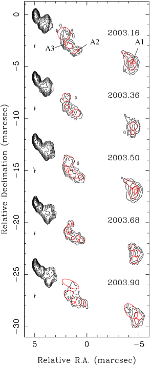
Figure 1: Naturally weighted final CLEAN images of 3C 273 at 43 GHz. Contour levels are represented by geometric series $c_{0}(1,...,2^{n})$, where $c_{0}$ is the lowest contour level corresponding to 5 times the off-source rms noise, which is given in Table 1 together with the restoring beam size and peak intensity for each image. Overlaid on the contour images are model-fit components in the outer part of the jet, and three prominent components are marked with A1–A3. The model-fit components located within the inner 2.5 mas from the core are shown in Fig. 2. See the on-line edition for a colour version of the figure.

Table 1: Parameters of the images in Fig. 1

Epoch	$\Theta_{b,\textrm{\scriptsize{maj}}}$	$\Theta_{b,\textrm{\scriptsize{min}}}$	P.A.	$\sigma(I)$	$I_{\textrm{\scriptsize{peak}}}$
[yr]	[mas]	[mas]	[$\degr$]	[mJy beam-1]	[mJy beam-1]
2003.16	0.44	0.18	-7.1	2.4	3961
2003.36	0.40	0.18	-3.5	2.2	2750
2003.50	0.43	0.19	-4.6	2.0	2600
2003.68	0.39	0.17	-6.3	1.7	2241
2003.90	0.44	0.18	-5.5	2.4	1997

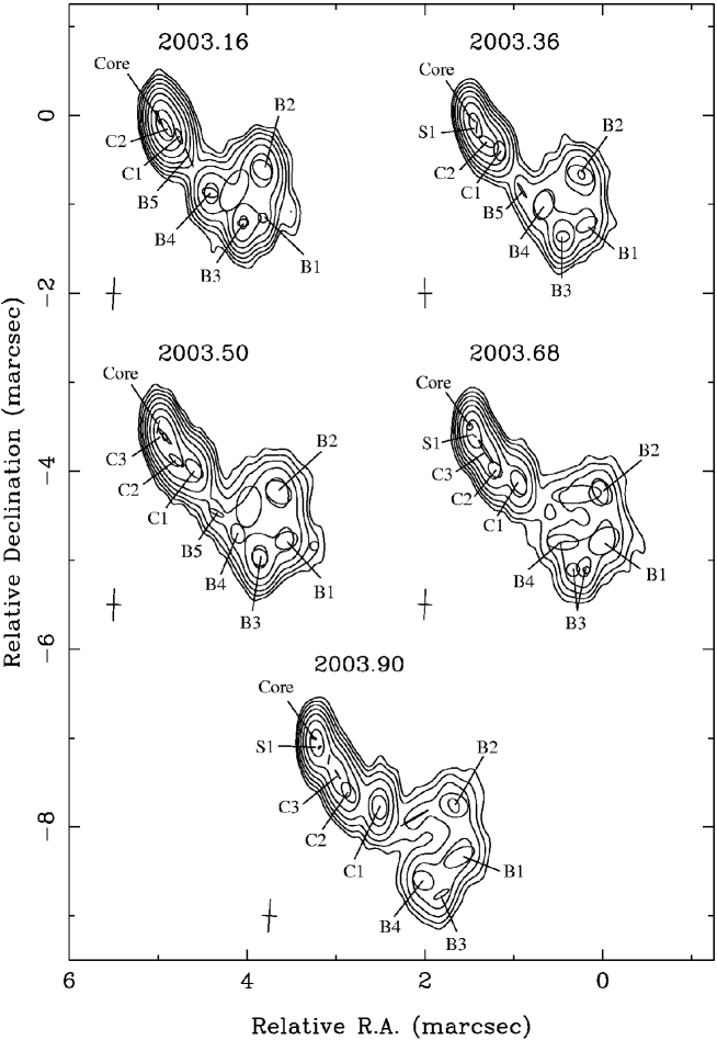
Figure 2:  Gaussian model components within 2.5 mas from the core and their convolution with a Gaussian beam corresponding to uniformly weighted ($u$,$v$) data with residuals added. Table 3 lists restoring beam sizes, peak intensities and off-source rms noise levels. Contour levels are represented by geometric series $c_{0}(1,...,2^{n})$, where $c_{0}$ is the lowest contour level corresponding to 5 times the off-source rms noise.

The final CLEAN images of 3C 273 (Fig. 1) are not easy to parameterise for quantitative analysis of e.g. proper motions and flux density evolution of different regions in the jet. To make a quantitative analysis feasible, we fitted models consisting of a number of elliptical and circular Gaussian components to fully self-calibrated visibility data (i.e. in the ($u$,$v$)-plane) using the “modelfit” task in Difmap. We sought to obtain the simplest model that gave a good fit to the visibilities and produced, when convolved with the restoring beam, a brightness distribution similar to that of the CLEAN image. 3C 273 is a complex source with a number of details, and due to its structure that could not easily be represented by well-separated, discrete components, model-fitting proved to be rather difficult. Due to this complexity, we added more constraints to the fitting process by demanding consistency between epochs, i.e. most components should be traceable over time. The final models show a good fit to the visibility data, and they nicely reproduce the structure in the CLEAN images (compare Figs. 1 and 2, the first showing CLEAN images and the latter presenting model components convolved with a Gaussian beam). However, these models (like any result from the model-fitting of the VLBI data) are not unique solutions, but rather show one plausible representation of the data.

Reliable estimation of uncertainties for parameters of the model fitted to VLBI data is a notoriously difficult task. This is due to loss of knowledge about the number of degrees of freedom in the data, because the data are no longer independent after self-calibration is applied. This makes the traditional $\chi^{2}$-methods useless, unless a well-justified estimate of degrees of freedom can be made. Often there is also strong interdependency between the components – for instance, adjacent components’ sizes and fluxes can be highly dependent on each other. This can be solved by using a method first described by Tzioumis et al. (tzi89 (1989)), where the value of the model parameter under scrutiny is adjusted by a small amount and fixed. The model-fitting algorithm is then run and results are inspected. This cycle is repeated until a clear discrepancy between the model and the visibilities is achieved. Difwrap (Lovell lov00 (2000)) is a program to automatically carry out this iteration, and we have used it to assess uncertainties for parameters of the model components. However, there is a serious problem also with this approach. Since the number of degrees of freedom remains unknown, we cannot use any statistically justified limit to determine what is a significant deviation from the data; we must rely on highly subjective visual inspection of the visibilities and of the residual map. We found that a reasonable criterion for a significant discrepancy between the data and model is the first appearance of such an emission structure, which we would have cleaned, had it appeared during the imaging process. For faint components, the parameters can change substantially with insignificant increase in the difference between the model and the visibilities, and hence, with low flux components we cannot rely on the results given by Difwrap, but we need to use other means to estimate the uncertainties. The above-described procedure for determination of uncertainties in model parameters does not address errors arising from significant changes in the model (e.g. changes in the number of components) or from imaging artefacts created by badly driven imaging/self-calibration iteration.

Homan et al. (hom01 (2001)) estimated the positional errors of the components by using the variance about the best-fit proper motion model. We applied their method to our data in order to estimate the positional uncertainties of weak components and to check the plausibility of the errors given by Difwrap for stronger components. We have listed the average positional error $\langle\Delta r_{DW}\rangle$ from the Difwrap analysis and the rms variation about the best-fit proper motion model $\sigma(r)$ for each component that could be reliably followed between the epochs in Table 2. The errors are comparable – for components B1–B4 they are almost identical and for components C1–C3 the uncertainties obtained by Difwrap are 0.01–0.02 mas larger than the rms fluctuations about the proper motion model. Diffuse components A1, A2 and A3 have Difwrap positional errors approximately twice as large as the variance about the best-fit model. We conclude that Difwrap yields reliable estimates for the positional uncertainties of the compact and rather bright components. As was mentioned earlier, it is difficult to obtain an error estimate for weak components with this method, and for diffuse components, the errors seem to be exaggerated. The average errors given in Table 2 agree well with the often quoted “$1/5$ of the beam size” estimate for positional accuracy of the model components (e.g. Homan et al. hom01 (2001), Jorstad et al. jor05 (2005)).

Table 2: Average positional uncertainties for the model components from the Difwrap ($\langle\Delta r_{DW}\rangle$) and from the variance analysis ($\sigma(r)$)

Component	$\langle\Delta r_{DW}\rangle$	$\sigma(r)$
	[mas]	[mas]
C1	0.03	0.01
C2	0.04	0.02
C3	0.04	0.02
B1	0.04	0.04
B2	0.03	0.03
B3	0.05	0.05
B4	0.05	0.03
B5	–	0.06
A1	0.10	0.05
A2	0.11	0.06
A3	0.06	0.02

Uncertainty in the flux density of a Gaussian component strongly depends on possible “flux leakage” between adjacent components, which is, in principle, taken into account in the Difwrap analysis. This flux leakage results in large and often asymmetric uncertainties, as can be seen in Figs. 11 and 12, where flux density evolution of the individual components is presented. The error bars in the figures correspond to the total uncertainty in the component flux density, where we have quadratically added the model error given by Difwrap and a 5% amplitude calibration error. The errors are on average 10% for moderately bright and rather isolated components with no significant flux leakage from other components, and $\sim 15$% for components with the leakage problem. For some bright and well-isolated components, flux density errors less than 10% were found, but in general uncertainties reported here are larger than those obtained by the $\chi^{2}$-method, which does not take into account the interdependency between nearby components’ flux densities (e.g. Jorstad et al. jor01 (2001)). Naturally, the caveat in the Difwrap method is the subjective visual inspection needed to place the error boundaries, but we note that Homan et al. (hom02 (2002)), who estimated flux density errors by examining the correlation of flux variations between two observing frequencies and taking an uncorrelated part as a measure of uncertainty, found flux density errors ranging from 5% to 20% at 22 GHz with 5%–10% being typical values for well-defined components. Our error estimates for component flux densities seem to agree with these values.

Uncertainties in the component sizes were also determined with Difwrap. Plausible values for errors were found only for bright components, and again, asymmetric uncertainties emerged commonly. The uncertainties in the size of the major axis of the component ranged from 0.01 mas to 0.15 mas corresponding to approximately 5%–30% relative uncertainty. Errors in the component axial ratios were difficult to determine with Difwrap, and results were obtained only for a small number of components. The axial ratio uncertainties range from 0.05 to 0.20, corresponding to a relative uncertainty of about 20%–60%. The large errors in the component sizes are again due to “leakage” between adjacent components. For well-isolated components, uncertainties in size would be smaller.

3 The structure of the parsec scale jet

Table 3: Parameters of the images in Fig. 2

Epoch	$\Theta_{b,\textrm{\scriptsize{maj}}}$	$\Theta_{b,\textrm{\scriptsize{min}}}$	P.A.	$\sigma(I)$	$I_{\textrm{\scriptsize{peak}}}$
[yr]	[mas]	[mas]	[$\degr$]	[mJy beam-1]	[mJy beam-1]
2003.16	0.37	0.17	-3.1	4.0	3833
2003.36	0.34	0.16	1.0	6.4	2605
2003.50	0.37	0.17	-1.8	3.7	2432
2003.68	0.35	0.16	-3.1	4.7	2242
2003.90	0.38	0.16	-3.7	4.1	1918

In our 43 GHz, high dynamic range images (Fig. 1; see also Table 1) we can track the jet up to a distance of $\sim 11$ mas from the core. The “wiggling” structure reported in several other studies (e.g. Mantovani et al. man99 (1999), Krichbaum et al. kri90 (1990), Bååth et al. baa91 (1991), Zensus et al. zen88 (1988)) is evident also in our images – the bright features are not collinear.

At all epochs, we consider the compact, easternmost component as the stationary radio core, and all proper motions are measured relative to it. As can be seen from Fig. 2, the innermost region “C” with the core and several departing components (C1–C3) extends about 1 mas to south-west. Besides the core, there is also another stationary component, S1, located $\sim 0.15$ mas from the core. Identification of the components close to the core over the epochs is problematic due to the number of knots close to each other, and also because new ejections are going on during our observing period. We have plotted the components within 1.5 mas from the core in Fig. 3 with the size of the symbol indicating the relative flux of each Gaussian component. The figure shows four moving components (C1–C3 and B5), and two stationary components (the core and S1), with consistent flux evolution. The figure also confirms that component C3 is ejected from the core during our monitoring period. Components C1–C3 may not necessarily represent independent and distinct features, but they also can be interpreted as a brightening of the inner jet – e.g. due to continuous injection of energetic particles in the base of the jet. VLBI data with better angular resolution could settle this, but, unfortunately, our 86 GHz observations suffer from the loss of the longest VLBA baselines, and thus, they cannot provide the necessary resolution. However, this should not affect the following kinematical analysis.

In the complex emission region at about 1–2.5 mas to southwest from the core, the jet is resolved in the direction transverse to the flow. We have identified five components (B1–B5) that are traceable over the epochs. The components can be followed from epoch to epoch in Fig. 2. B3 is represented by two Gaussian components at the fourth epoch, and B5 is not seen after the third epoch, but otherwise we consider that our identification is robust. B4 seems to catch up with the slower knot B3 and collides with it (see Figs. 6 and 7).

The jet broadens significantly after $\sim 1.5$ mas and, as shown later in Sect. 4, the trajectory of the component B1 does not extrapolate to the core (Fig. 2). We discuss the possible explanations for this anomalous region “B” in Sect. 6. Farther down the jet, there are two more emission regions visible in the 43 GHz images, both of them showing a curved structure (Fig.1). The first one is located 3–6 mas southwest of the core and we have identified two components A2 and A3 in it. This feature likely corresponds to knots B1, bs, b1, B2 and b2 of Jorstad et al. (jor05 (2005)), with our A2 being their B1/bs, and our A3 being their B2. However, this cross-identification is not certain, since the region is complex and, as described in Jorstad et al. (jor05 (2005)), it contains components with differing speeds and directions as well as secondary components connected to the main disturbances. The second emission region in the outer part of the jet is located at 9–11 mas from the core, and we call this component with a curved shape A1 (Fig. 1).

4 Kinematics of the jet

The data allow us to follow the evolution of the components identified in the previous section, and to measure their proper motion, which is the basis for analysing physical properties of the jet. We follow the practice of Jorstad et al. (jor05 (2005)), and define the average proper motion as a vector $(\langle\mu\rangle,\langle\Phi\rangle)$, where $\langle\mu\rangle=\sqrt{\langle\mu_{\mathrm{RA}}\rangle^{2}+\langle\mu_{\mathrm{Dec}}\rangle^{2}}$ is the mean angular speed and $\langle\Phi\rangle=\tan^{-1}\big{(}\frac{\langle\mu_{\mathrm{RA}}\rangle}{\langle\mu_{\mathrm{Dec}}\rangle}\big{)}$ is the direction of motion. In all but one case, the average coordinate motions $\langle\mu_{\mathrm{RA}}\rangle$ and $\langle\mu_{\mathrm{Dec}}\rangle$ are obtained by a linear least-squares fit to the relative (RA,Dec) positions of a component over the observation epochs. For component C1, a second-order polynomial was fitted instead of a first-order one, because it reduced the $\chi^{2}$ for the RA-coordinate fit from 4.7 (with 3 degrees of freedom) to 0.2 (with 2 degrees of freedom). Also, the (RA,Dec)-plot in Fig.4 indicates a non-ballistic trajectory for component C1. The amount of acceleration measured for C1 is $0.21\pm 0.18$ mas yr^-2 – a marginal detection (Fig. 5).

Table 4: Proper motion results

Component	$S_{\mathrm{max}}$ [Jy]	$\langle\Phi\rangle$ [∘]	$\langle\mu\rangle$ [mas yr-1]	$\langle\beta_{\mathrm{app}}\rangle$ [h-1 c]	$T_{0}$ [yr]
S1	1.28	30.6	$0.05\pm 0.05$	$0.4\pm 0.4$	–
C1	1.34	$-139.4\pm 0.3$	$1.01\pm 0.05$	$7.3\pm 0.4$	$2002.76\pm 0.04$
C2	4.38	$-150.5\pm 0.7$	$0.79\pm 0.07$	$5.7\pm 0.5$	$2002.97\pm 0.05$
C3	3.00	$-147.5\pm 1.0$	$0.95\pm 0.13$	$6.9\pm 0.9$	$2003.36\pm 0.03$
B1	0.80	$-115.1\pm 0.7$	$0.71\pm 0.06$	$5.1\pm 0.4$	–
B2	1.89	$-113.3\pm 0.6$	$0.63\pm 0.05$	$4.6\pm 0.4$	$2001.09\pm 0.19$
B3	1.69	$-141.2\pm 0.5$	$0.99\pm 0.06$	$7.2\pm 0.4$	$2001.63\pm 0.11$
B4	1.13	$-141.3\pm 0.4$	$1.34\pm 0.07$	$9.7\pm 0.5$	$2002.40\pm 0.06$
B5	0.25	$-149.6\pm 1.1$	$1.80\pm 0.25$	$13.0\pm 1.8$	$2002.83\pm 0.10$
A1	0.87	$-116.8\pm 1.0$	$0.95\pm 0.13$	$6.9\pm 0.9$	$1992.2\pm 1.5$
A2	0.32	$-108.0\pm 1.2$	$1.17\pm 0.18$	$8.5\pm 1.3$	–
A3	0.48	$-126.2\pm 2.3$	$1.07\pm 0.32$	$7.8\pm 2.3$	$1999.4\pm 1.2$

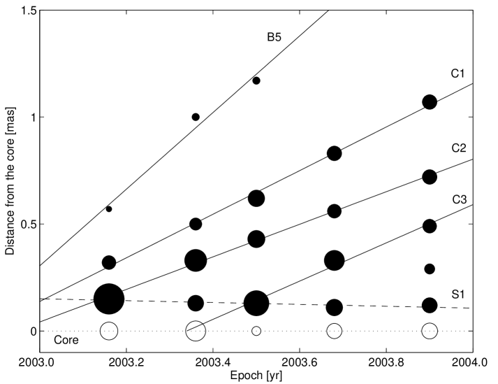
Figure 3: Separation of the components from the core vs. epoch of observation for the components located within 1.5 mas from the core. The size of the circle is proportional to square root of the flux density. The solid lines represent the best linear approximation of the data for moving components, while the dashed line is the best-fit to the positions of stationary component S1. We used linear fits here for all components, although C1 is better fitted with a second-order polynomial as shown in Fig. 5. The open circles correspond to the core.

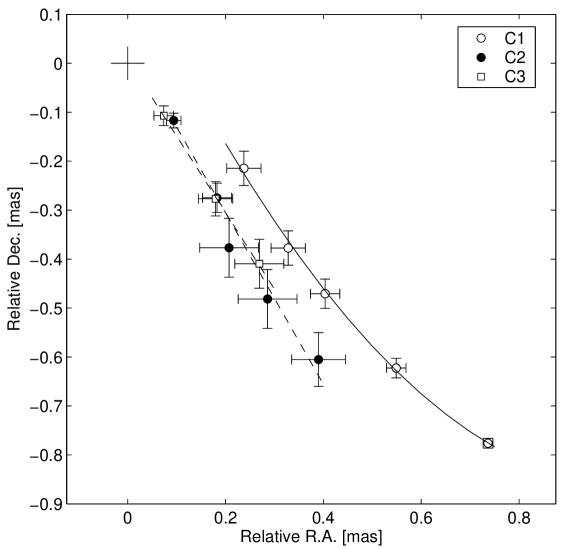
Figure 4: Trajectories of components C1–C3. The symbols show the measured positions of the components. The solid line is the best-fit curve for component C1 and the dashed lines show linear trajectories fitted for components C2 and C3. The plus sign marks the core.

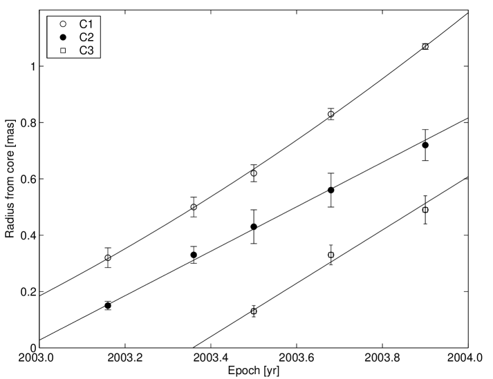
Figure 5: Separation of components C1–C3 from the core vs. epoch of observation. The solid lines(curve) represent the best-fit straight lines(second-order polynomial) describing the component motion (see Table 4).

In Figs. 4, 6, and 8, we have plotted the trajectories in the (RA,Dec)-plane for components C1–C3, B1–B5 and A1–A3, respectively. As can be seen from these figures, there are three components showing non-radial motion, C1, B1 and A2. As was discussed earlier, C1 seems to have a curved trajectory, while B1 and A2 have straight trajectories, which, however, do not extrapolate back to the core. B1 has an especially interesting path, since its motion seems to be parallel to that of B2, but clearly deviating from those of B3 and B4, which have a direction of $\sim 25\degr$ more southern than B1. Also, B1 and B2 have similar speeds, while B3 and B4 are both faster. B1 might have formed from B2 or B3, possibly through an interaction between relativistic shocks connected with these components and the underlying flow, or it might have changed its trajectory.

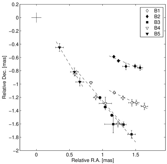
Figure 6: Trajectories of components B1–B5. The symbols show measured positions of components, and the best-fit linear trajectories are represented by the dashed lines. The plus sign marks the core. Note that the trajectory for component B1 clearly does not extrapolate back to the core.

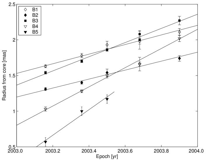
Figure 7: Separation of components B1–B5 from the core vs. epoch of observation. The solid lines represent the best-fit to the component motion (see Table 4).

In Figs. 5, 7, and 9, we have plotted the separation from the core as a function of time for the components. Table 4 lists the maximum measured flux density, $S_{\mathrm{max}}$, the average proper motion, $(\langle\mu\rangle,\langle\Phi\rangle)$, the apparent superluminal speed, $\beta_{\mathrm{app}}$, and the extrapolated epoch of zero-separation, $T_{0}$, for the components. Ejection time is not given for the component S1, which is stationary, nor the components B1 and A2, whose trajectories do not extrapolate back to the core. The uncertainties in the average proper motion are derived from the uncertainties of the fitted polynomial coefficients.

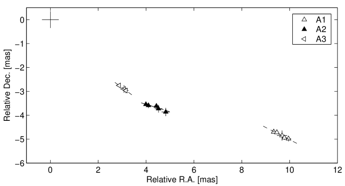
Figure 8: Trajectories of components A1–A3. The symbols show measured positions of components, and the best-fit linear trajectories are represented by the dashed lines. The plus sign marks the core.

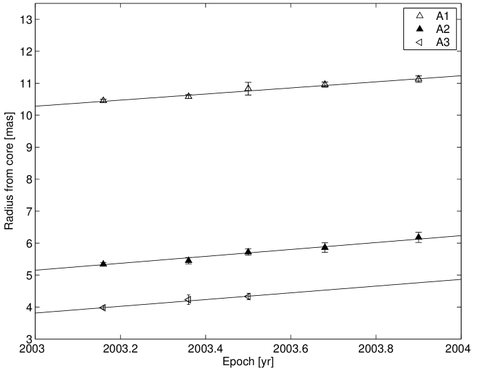
Figure 9: Separation of components A1–A3 from the core vs. epoch of observation. The solid lines represent the best-fit to the component motion (see Table 4).

The superluminal velocities for the moving components range from 4.6 $h^{-1}$ c to 13.0 $h^{-1}$ c (with $H_{0}=100h$). This range of velocities is similar to those previously reported by e.g. Zensus et al. (zen90 (1990)), Krichbaum et al. (kri00 (2000)), and Jorstad et al. (jor05 (2005)). The largest observed apparent speed, 13.0 $h^{-1}$ c for B5, is based only on three epochs of observations, and the component is weak having flux density below 0.25 Jy. This renders the kinematical result somewhat uncertain, and the high proper motion of B5 needs to be confirmed by checking against the lower frequency and polarisation data in the follow-up papers. Components B1 and B2 with $\Phi\approx-115\degr$ have velocities that are significantly slower than those of the more southern components, B3–B5, with $\Phi\approx-145\degr$. A similar velocity gradient transverse to the jet, with components in the northern side having lower speeds, has been reported by Jorstad et al. (jor05 (2005)).

5 Physical parameters of the jet

Doppler boosting has an effect on most of the observable properties of a relativistic jet. Hence, in order to compare observations with predictions from theory, the amount of Doppler boosting needs to be measured first. Unfortunately, the Doppler factor of the jet,

$$\delta=[\Gamma(1-\beta\cos\theta)]^{-1},$$ (1)

where $\Gamma=1/\sqrt{1-\beta^{2}}$ is the bulk Lorentz factor and $\theta$ is the angle between the jet flow direction and our line of sight, is difficult to measure accurately (see Lähteenmäki & Valtaoja lah99b (1999) for a discussion of problems in determining $\delta$). In this section, we narrow down the possible range of values for $\delta$, $\Gamma$ and $\theta$ of 3C 273 in early 2003, so that meaningful comparison with the hard X-ray flux measured by the INTEGRAL satellite can be made (Paper II).

The apparent component velocities $\beta_{\mathrm{app}}$ given in Table 4 already put limits on $\Gamma$ and $\theta$. Namely, for all $\beta_{\mathrm{app}}>1$ there is a lower limit for the Lorentz factor $\Gamma_{\mathrm{min}}=\sqrt{1+\beta_{\mathrm{app}}^{2}}$ and an upper limit for the viewing angle, $\sin\theta_{\mathrm{max}}=2\beta_{\mathrm{app}}/(1+\beta_{\mathrm{app}}^{2})$. $\Gamma_{\mathrm{min}}$ and $\theta_{\mathrm{max}}$ for each component are listed in Table 5 (assuming $h=0.71$). These values are calculated using lower limits of $\beta_{\mathrm{app}}$. As can be seen from Table 5, the minimum value for $\Gamma$ in the region close to the VLBI core in 2003 (components C1–C3) is 7.4 and $\theta_{\mathrm{max}}=15.5^{\circ}$.

Table 5: Limits for $\Gamma$ and $\theta$

Component	$\Gamma_{\mathrm{min}}$	$\theta_{\mathrm{max}}$ [$\degr$]
C1	9.8	11.7
C2	7.4	15.5
C3	8.5	13.5
B1	6.7	17.2
B2	6.0	19.2
B3	9.6	11.9
B4	13.0	8.8
B5	15.8	7.3
A1	8.5	13.5
A2	10.2	11.3
A3	7.8	14.7

5.1 Variability time scales and Doppler factors

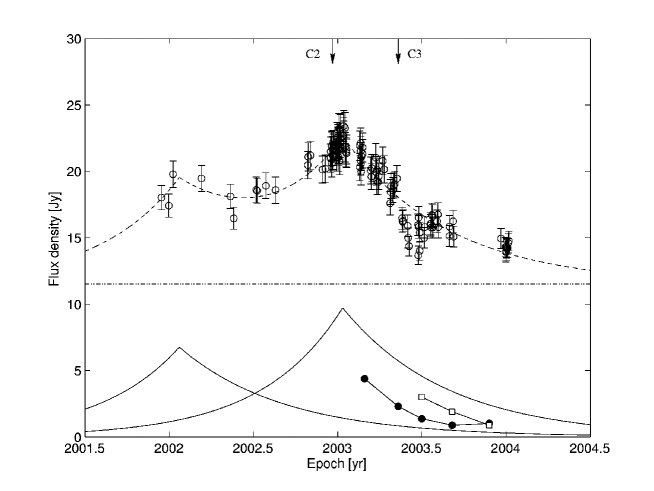
Figure 10:  Metsähovi total flux density curve of 3C 273 at 37 GHz with superposed exponential flare model fits. Open circles with error bars correspond to the total flux density measurements, the solid curves represent the two fitted flares, the dot-dashed line represents a constant baseline flux of 11.5 Jy, and the dashed line is the sum of the flares and the baseline. The flux density curves of two VLBI components showing flare-like behaviour in 2003, C2 (filled circles) and C3 (open squares) are also plotted in the figure. The extrapolated ejection epochs of these two components are marked with arrows.

37 GHz total flux density data from the Metsähovi Radio Observatory monitoring program for 2002–2004 is shown in Fig. 10. A small flare occured at the beginning of 2003. It has about four times smaller amplitude than the large outburst in 1991 (Robson et al. rob93 (1993)), making it only a minor but still useful event to estimate the variability brightness temperature and the Doppler factor of the jet, as we will show. As is clear from the ejection times listed in Table 4, components C1–C3 can be connected to this event. The flux density evolution of C2 (see Figs. 10 and 11) closely matches the flare in the Metsähovi flux density curve. C1 has an approximately stable flux density of $\sim 1$ Jy, which makes it a less likely counterpart to the flare, and C3, on the other hand, was ejected at the time when the flare was already fading. The flux density of the core increases at the second epoch and decreases considerably at the third (see Fig. 11), while the component C3 becomes distinct from the core at the same time. The flux density curve of C3 shows flare-like behaviour, possibly corresponding to a small rise in the single-dish flux density around July 2003. We interpret the rise in the core flux density at the second epoch and a sudden drop at the third epoch to be related to the ejection of C3. Based on the flux curves in Fig. 10, it seems to be a reasonable assumption that the flare seen in the single-dish flux density data in January 2003 is mainly caused by a recently ejected component C2.

Observed flux density variability – both in single-dish data and in the VLBI components – can be used to calculate the size of the emission region. In the shock-in-jet model for radio variability, the nearly symmetric flares observed at high radio frequencies (Teräsranta & Valtaoja ter94 (1994)) suggest that the flux density variability is controlled by light travel delays across the shocked region (Jorstad et al. jor05 (2005), Sokolov et al. sok04 (2004)) i.e. the flux density variability time scale defined as $\tau=dt/d\ln(S)$ corresponds to the light crossing time across the region. This is true if the light crossing time is longer than the radiative cooling time but shorter than the adiabatic cooling time. Jorstad et al. (jor05 (2005)) verified this by comparing flux density variability time scales calculated for VLBI components with time scales of variability in apparent sizes of the same components. They found that the majority of components had a shorter flux variability time scale than that predicted for adiabatic expansion, implying that at high radio frequencies the decay in flux density is driven by radiative cooling. The above assumption allows us to identify $\tau$ with the light-crossing time across the emission region and hence, to estimate the size of the region, which can be then compared with the size measured from the VLBI data to calculate the Doppler factor.

First, we estimate the variability time scale $\tau_{\mathrm{TFD}}$ from the total flux density data. In order to make a simple parametrisation of the flare in January 2003, we have decomposed the flux curve into a constant baseline and separate flares consisting of exponential rise, sharp peak and exponential decay (see Valtaoja et al. val99 (1999) for details). Model flares are of the form

$$\Delta S(t)=\left\{\begin{array}[]{ll}\Delta S_{\mathrm{max}}e^{(t-t_{\mathrm{peak}})/\tau_{\mathrm{TFD}}},&t<t_{\mathrm{peak}}.\\ \Delta S_{\mathrm{max}}e^{(t_{\mathrm{peak}}-t)/(1.3\tau_{\mathrm{TFD}})},&t>t_{\mathrm{peak}}.\end{array}\right.$$ (2)

Our best fit (dashed line) is presented in Fig. 10, consisting of two small flares and a constant baseline of 11.5 Jy. Parameters of this fit are given in Table 6. The variability time scale for the 2003 flare is $\tau_{\mathrm{TFD}}=175$ days. The uncertainty in $\tau_{\mathrm{TFD}}$ is rather hard to estimate, but according to Lähteenmäki et al. (lah99a (1999)), a conservative upper limit for $\sigma(\tau_{\mathrm{TFD}})\lesssim\tau_{\mathrm{TFD}}/4$. An angular size $a$ corresponding to $\tau_{\mathrm{TFD}}=175\pm 44$ d is given by

$$a=\frac{c\tau_{\mathrm{TFD}}(1+z)}{D_{\mathrm{L}}}\delta,$$ (3)

where $D_{\mathrm{L}}$ is luminosity distance:

$$D_{\mathrm{L}}=\frac{c(1+z)}{H_{0}}\xi(\Omega_{M},\Omega_{\Lambda},z),$$ (4)

with function $\xi$ given by

$$\xi(\Omega_{M},\Omega_{\Lambda},z)=\int_{0}^{z}\frac{dz^{\prime}}{\sqrt{(1+z^{\prime})^{2}(1+\Omega_{M}z^{\prime})-z^{\prime}(2+z^{\prime})\Omega_{\Lambda}}},$$ (5)

(this applies when $\Omega_{M}+\Omega_{\Lambda}=1$; see Carroll et al. car92 (1992)). For January 2003 flare, $a=(0.047\pm 0.012)\delta$ mas, which can be compared with the size of C2 measured from the VLBI data. The full width at half maximum (FWHM) size of the major axis of the Gaussian component C2 is $0.23\pm 0.04$ mas and the axial ratio is $\eta=0.29\pm 0.06$. Taking the geometric mean of major and minor axes and multiplying the result by 1.8, we get a size equivalent to an optically thin sphere, $a_{\mathrm{VLBI}}=0.22\pm 0.05$ mas. Comparison with $a$ from variability gives $\delta=4.7\pm 1.6$ for C2.

Table 6: Decomposition of the single-dish flux curve into self-similar flares

Flare	$t_{\mathrm{peak}}$ [year]	$\Delta S_{\mathrm{max}}$ [Jy]	$\tau_{\mathrm{TFD}}$ [days]
1	2003.03	9.72	$175\pm 44$
2	2002.06	6.76	$174\pm 44$
Constant baseline		11.5 Jy

The variability time scale can also be determined solely on the basis of flux density variability of a single VLBI component. As can be seen from Figs. 11 and 12, components B2, B3, B4, C2 and C3 show enough flux density variability that they can be used in estimating the variability time scale. The flux density time scales, $\tau_{\mathrm{VLBI}}$, the sizes at the time of maximum flux densities, $a_{\mathrm{VLBI}}$ (with geometry of an optically thin sphere assumed, i.e. the figures are multiplied by 1.8), and the calculated Doppler factors $\delta$ are presented in Table 7 for these components. In calculating $\tau_{\mathrm{VLBI}}$ and $\delta$, we have taken into account the asymmetric uncertainties in flux densities and sizes of several components (see e.g. D’Agostini (ago04 (2004)) for a short review about asymmetric uncertainties and their correct handling). The figures given in Table 7 are probabilistic expected values, not “best values” obtained by direct calculation, and the uncertainties correspond to probabilistic standard deviations.

A non-linear dependence of the output quantity $Y$ on the input quantity $X$ in a region of few standard deviations around the expected value of $X$ is another source of asymmetric uncertainties, which also needs to be properly taken into account when doing calculations with measured quantities. In this paper, when calculating derived quantities like brightness temperature, which has a strongly non-linear dependence on the size of the component, we have used a second-order approximation for the error propagation formula instead of the conventional linear one. Moreover, the non-linearity does not only affect the errors, but it can also shift the expected value of $Y$ with respect to the “best value” obtained by direct calculation (D’Agostini ago04 (2004)). In the following, for all the derived quantities, expected values and standard deviations are reported instead of directly calculated values, since they are much more useful for any statistical analysis.

Table 7: Variability time scales and Doppler factors from the VLBI data

Component	$\tau_{\mathrm{VLBI}}$ [days]	$a_{\mathrm{VLBI}}$ [mas]	$\delta$
C2	$110\pm 30$	$0.22\pm 0.05$	$7.5\pm 2.6$
C3	$120\pm 10$	$0.12\pm 0.04$	$4.1\pm 1.4$
B2	$110\pm 20$	$0.36\pm 0.05$	$12.2\pm 2.8$
B3	$160\pm 30$	$0.18\pm 0.04$	$4.2\pm 1.7$
B4	$100\pm 30$	$0.23\pm 0.05$	$8.6\pm 3.2$

The two variability time scales for C2, estimated from the total flux density and from the VLBI data, differ by 60 days, which affects the calculated Doppler factors – from the total flux density variability we get $\delta(C2)=4.7\pm 1.6$ as compared to $\delta(C2)=7.5\pm 2.6$ calculated from the variability in the VLBI data. A weighted average of these, $\delta(C2)=5.5\pm 1.9$, agrees well with other Doppler factor values for 3C 273 derived elsewhere: $\delta_{var}=5.7$ (Lähteenmäki & Valtaoja 1999), $\delta_{eq}=8.3$, $\delta_{SSC}=4.6$ (Güijosa & Daly gui96 (1996)), and $\delta_{SSC}=6.0$ (Ghisellini et al. ghi93 (1993)). The variability Doppler factors of other components listed in Table 7 vary significantly, with C3 and B3 having the smallest values, $\delta\sim 4$, and B2 having the highest, $\delta(B2)=12.2\pm 2.8$. This is not very surprising, since also the apparent velocities of these components differ considerably.

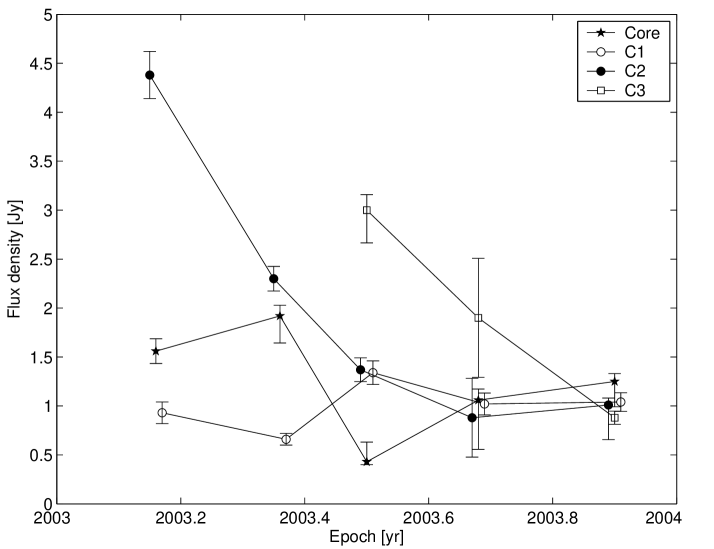
Figure 11: Flux density evolution for the core and components C1–C3. The asymmetric error bars are mainly due to interdependencies between flux densities of close-by components.

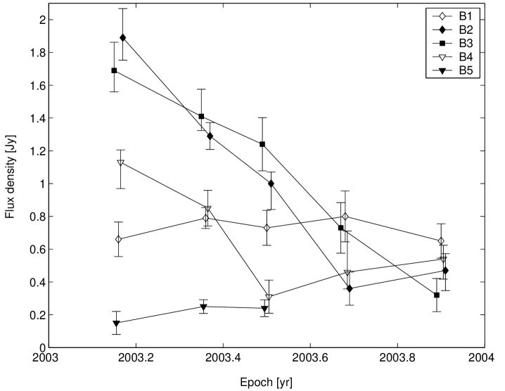
Figure 12: Flux density evolution for components B1–B5.The asymmetric error bars are mainly due to interdependencies between flux densities of close-by components.

5.2 Brightness temperatures and equipartition

Brightness temperature is another quantity of interest in sources like 3C 273. From the total flux density variability, we can estimate the variability brightness temperature (Lähteenmäki et al. lah99a (1999))

$$T_{b,\mathrm{var}}=5.28\times 10^{20}\cdot h^{-2}\frac{\Delta S_{\mathrm{max}}}{\nu^{2}\tau^{2}_{\mathrm{TFD}}}(1+z)\xi(\Omega_{M},\Omega_{\Lambda},z)^{2},$$ (6)

where $\nu$ is the observation frequency in GHz, $z$ is redshift, $\Delta S_{\mathrm{max}}$ is the maximum amplitude of the outburst in Janskys, and $\tau_{\mathrm{TFD}}$ is the observed variability timescale in days. The numerical factor in equation 6 comes from assuming that the component is an optically thin, homogeneous sphere. Lähteenmäki et al. (lah99a (1999)) estimate a conservative upper limit to the error in $T_{b,\mathrm{var}}$ to be $\Delta T/T<0.50$. For the flare in January 2003, $T_{b,\mathrm{var}}=(6.6\pm 3.3)\times 10^{12}$ K.

The observed variability brightness temperature is proportional to $\delta^{3}$, i.e. $T_{b,\mathrm{var}}=T_{b,\mathrm{int}}\delta^{3}$. Using $\delta=5.5\pm 1.9$, obtained earlier for component C2, we get a value $T_{b,\mathrm{int}}\approx(8\pm 6)\times 10^{10}$ K of intrinsic brightness temperature (the strong non-linear dependence of $T_{b,\mathrm{int}}$ on $\delta$ shifts the expected value of $T_{b,\mathrm{int}}$ significantly from the directly calculated “best value” of $\approx 4\times 10^{10}$ K; D’Agostini ago04 (2004)), which is consistent with the source being near equipartition of energy between the radiating particles and the magnetic field. According to Readhead (rea94 (1994)) the equipartition brightness temperature, $T_{b,\mathrm{eq}}$, depends mainly on the redshift of the source and weakly on the observed optically thin spectral index, the peak flux density and the observed frequency at the peak. For the redshift of 3C 273, $T_{b,\mathrm{eq}}\sim 8\times 10^{10}$ K for any reasonable values of $\alpha$, $S_{m}$ and $\nu_{m}$. This exactly matches the $T_{b,\mathrm{int}}$ calculated for the January 2003 flare, indicating that near the core the source could have been in equipartition. Our result is consistent with the findings of Lähteenmäki et al. (lah99a (1999)), who have shown that during high radio frequency flares all sources in their sample have intrinsic brightness temperature close to the equipartition value.

Interferometric brightness temperatures of the components are also of interest. The maximum brightness temperature for an elliptical component with a Gaussian surface brightness profile is

$$T_{b,\mathrm{VLBI}}=1.22\times 10^{12}\cdot\frac{S_{\mathrm{VLBI}}(1+z)}{\eta a_{\mathrm{maj}}^{2}\nu^{2}}$$ (7)

where $S_{\mathrm{VLBI}}$ is the flux density in Janskys, $\nu$ is the observed frequency in GHz, $z$ is redshift, $a_{\mathrm{maj}}$ is the FWHM size of the major axis in mas, and $\eta$ is the axial ratio of the component. In order to consider a surface brightness distribution, which is more physical than a Gaussian, we convert the Gaussian brightness temperature to an optically thin sphere brightness temperature by multiplying the former by a factor of 0.67. Table 8 lists the maximum interferometric brightness temperatures for components within 2.5 mas from the core and with non-zero areas. Again, we have taken into account the effect of asymmetric errors in $S_{\mathrm{VLBI}}$, $a_{\mathrm{maj}}$ and $\eta$, as well as the non-linearity of the equation 7, for error propagation. The table also contains the average Doppler factor and $T_{b,\mathrm{int}}$ calculated by dividing $T_{b,\mathrm{VLBI}}$ by $\delta$. $T_{b,\mathrm{int}}$ for C2 given in Table 8 differs from $(8\pm 6)\times 10^{10}$ K that was quoted earlier, because it is calculated using the interferometric brightness temperature instead of variability brightness temperature. However, the difference is not significant, considering the overall uncertainties in measuring $T_{b,\mathrm{int}}$

Table 8: Component properties

Component	$T_{b,\mathrm{VLBI}}$ [K]	$\delta$	$T_{b,\mathrm{int}}$ [K]	$\Gamma$	$\theta$ [$\degr$]
C1	$(7.9\pm 5.5)\times 10^{10}$	–	–	–	–
C2	$(1.7\pm 0.7)\times 10^{11}$	$5.5\pm 1.9$	$(3\pm 2)\times 10^{10}$	$9.8\pm 3.2$	$9.8\pm 2.1$
C3	$(3.4\pm 1.4)\times 10^{11}$	$4.1\pm 1.4$	$(8\pm 3)\times 10^{10}$	$14\pm 5$	$10.0\pm 1.5$
B1	$(4.0\pm 2.3)\times 10^{10}$	–	–	–	–
B2	$(2.5\pm 0.7)\times 10^{10}$	$12.2\pm 2.8$	$(2\pm 1)\times 10^{9}$	$8.0\pm 1.0$	$4.3\pm 1.6$
B3	$(1.2\pm 0.7)\times 10^{11}$	$4.2\pm 1.7$	$(3\pm 2)\times 10^{10}$	$17\pm 7$	$9.7\pm 0.8$
B4	$(4.0\pm 1.8)\times 10^{10}$	$8.6\pm 3.2$	$(5\pm 2)\times 10^{9}$	$18\pm 8$	$6.0\pm 1.2$

5.3 Lorentz factors and viewing angles

Since we have measured $\delta$ and $\beta_{\mathrm{app}}$ for a number of components, it is possible to calculate the values of $\Gamma$ and $\theta$. The Lorentz factor is given by equation

$$\Gamma=\frac{\beta_{\mathrm{app}}^{2}+\delta^{2}+1}{2\delta}$$ (8)

and the angle between the jet and our line of sight by equation

$$\theta=\arctan\frac{2\beta_{\mathrm{app}}}{\beta_{\mathrm{app}}^{2}+\delta^{2}-1}.$$ (9)

The most reliable value of the Doppler factor was obtained for component C2. With $\beta_{\mathrm{app}}(C2)=8.0\pm 0.7$ and $\delta(C2)=5.5\pm 1.9$, we get $\Gamma=9.8\pm 3.2$ and $\theta=9.8\pm 2.1\degr$.

In Table 8 we have gathered Lorentz factors and viewing angles also for other components besides C2. The results indicate that a transverse velocity gradient across the jet does exist, even when the viewing angle difference is taken into account. B2 has $\Gamma=8$, while B3 and B4 show $\Gamma\sim 17$, and even the lower limit of Lorentz factor for B4 is larger than $\Gamma(B2)$ (see Table 5).

6 Discussion

3C 273 is the closest quasar, and due to its proximity it provides one of the best chances to study the physics of a strong relativistic outflow in detail. The jet in 3C 273 is complicated, with a number of details which would be smoothed away if the source was located at higher redshift. This complexity also makes it hard to interpret. For instance, several interferometric studies on the parsec scale jet of 3C 273 in the 1980s and 1990s have reported a “wiggling” structure with time-variable ejection angles and component velocities (e.g. Zensus et al. zen88 (1988), Krichbaum et al. kri90 (1990), Bååth et al. baa91 (1991), Abraham et al. abr96 (1996), Mantovani et al. man99 (1999)). In the following, we will explore some possible scenarios that could lie behind the observed curving structure, and discuss the observational evidence for and against them.

6.1 Precession of the jet nozzle

Abraham & Romero (abr99 (1999)) proposed a simple model of a ballistic jet with a precessing nozzle to explain the variable ejection angles and component velocities. Their model fits well the early VLBI data describing components ejected between 1960–1990. To compare our more recent high frequency data with their model, we have plotted the apparent speeds and directions of motion for the components as a function of their ejection epochs in Fig. 13 (excluding the faint B5). Overlaid in the figure are the predicted curves from the Abraham & Romero model. It is clear that the component velocities and directions show much faster variations than the precession model with a period of $\sim 15$ years predicts. No periodicity can be claimed on the basis of our data, although the apparent velocities may show pseudo-sinusoidal variation. However, the directions of the components’ proper motions show no clear pattern, and the apparent direction changes as fast as $\sim 30\degr$ in half a year.

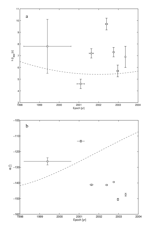
Figure 13: Apparent superluminal velocities (panel a) and direction of motion (panel b) of the bright superluminal components ejected between 1998 and 2003 as a function of ejection epoch. The dashed curves represent the prediction of the precession model by Abraham & Romero (abr99 (1999)). The horizontal error bars represent the uncertainty in ejection epochs.

There is one important difference between our data and that used by Abraham & Romero (abr99 (1999)) to construct their model. Most observations cited in their paper were carried out at lower frequencies (mainly 10.7 GHz) with significantly poorer resolution. Many of the components in our 43 GHz maps are small and often part of a larger emission structure, which is likely to show up as a single component on lower resolution maps. Such a component could show drastically different ejection angles than the individual features in it due to averaging. We have tested whether our data could fit the precession model of Abraham & Romero, were it observed with poorer resolution. The 43 GHz uv-data were tapered into a resolution comparable to VLBA observations at 10.7 GHz and then model-fitted (an example is shown in Fig. 14). In Fig. 15 we have plotted the apparent velocities and directions of motion for three prominent components in the tapered data as a function of their ejection epochs. We have also included the data from Abraham & Romero (abr99 (1999)), scaled to the cosmology used in this paper, and superimposed their precession model to the figure. As can be seen, we cannot exclude the possibility that the average jet direction changes periodically, and that it can be approximately described by the Abraham & Romero model.

Figure 14: Image showing strongly tapered uv-data of the third epoch (2003.50) observation. We have tapered the 43 GHz data to a resolution which corresponds to observations at 10.7 GHz with a similar array of antennas.

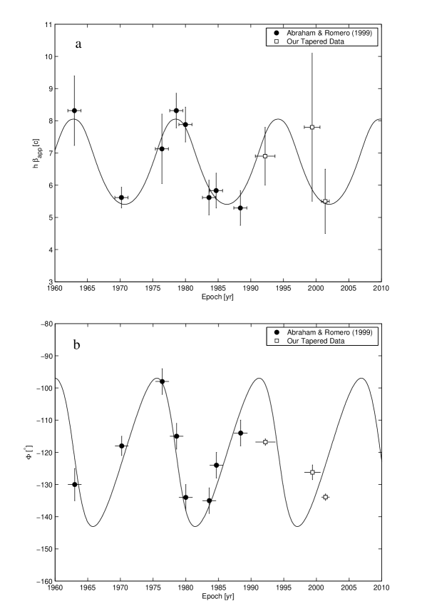
Figure 15: Apparent superluminal velocities (panel a) and direction of motion (panel b) of the strong superluminal components as a function of ejection epoch. We have plotted in the figure low frequency data collected by Abraham & Romero (abr99 (1999)) with $\beta_{\mathrm{app}}$ scaled to the cosmology used in this paper, and our 43 GHz data tapered to a resolution corresponding to observations made at 10.7 GHz. The solid curves represent the precession model of Abraham & Romero (abr99 (1999)).

6.2 Ballistic or not?

The simplest possible model describing proper motions in a relativistic jet is the one where knots ejected from the core move at constant velocity following a ballistic trajectory. On the contrary, non-ballistic motion in the jet implies a more complex physical system with dynamics governed by e.g. magnetic fields, fluid instabilities or interaction with the ambient medium.

Most of the components observed in our data follow, at least on a timescale of nine months, a straight path starting from the core with a constant velocity. However, there are a few important exceptions. Component C1 shows a curved trajectory with slight bending towards the north (Fig. 4). Its position at the last epoch deviates $\sim 0.11$ mas from the straight line path extrapolated from the first three epochs and it does not follow the path taken earlier by components B3–B5. Follow-up observations tracking the motion of C1 will show if the bending continues and C1 becomes a “northern component” with a trajectory similar to B2 or B3. The component B1 of Jorstad et al. (jor05 (2005)) has a curved trajectory with these characteristics, indicating that the behaviour of C1, if it actually continues to bend, is not unique. The other two exceptions to radial motion are components B1 and A2, which do not extrapolate back to the core. B1 lies $\sim 0.6$ mas south of B2 and moves parallel to it. This component may have been split from B3 or B2, or it may have changed its direction earlier – similarly to C1.

Several studies report non-ballistic motion in 3C 273. Kellermann et al. (kel04 (2004)) found a non-radial trajectory for one of the components in their 2 cm VLBA Survey monitoring, Homan et al. (hom01 (2001)) also reported a curved path for one component, and Jorstad et al. (jor05 (2005)) identified several knots following a bent trajectory. Fig. 5 in Krichbaum et al. (kri00 (2000)) is a very interesting plot, where the long term motion of 12 components is presented in the (RA,Dec)-plane. The components show slightly curved trajectories with both convex and concave shapes. It is apparent from this figure that had the components been followed only for a year, one would have described most of them as ballistic. This is in agreement with our data, and we consider it likely that several components have non-ballistic trajectories, although with large radii of curvature. One more piece of evidence supporting this view comes from the apparent opening angle of the jet. At 1–2 mas from the core, we can estimate the apparent opening angle of the jet from the motion directions of B2 and B3, yielding $28\degr$ in the plane of the sky. In a 5 GHz image taken at the first epoch, the jet is well-collimated up to 50 mas and its opening angle on the scale of 10–50 mas is significantly smaller than $28\degr$ (Paper II; preliminary 5 GHz data is published in Savolainen et al. sav04 (2004), see their Fig. 1). In the kpc scale jet, the half-power width remains constant (1.0″) from 13″to 20″along the jet implying highly collimated outflow and, again, a small opening angle (Conway et al. con93 (1993)). If the large observed opening angle of $28\degr$ at 1–2 mas from the core is not due to a rare event of changing jet direction (see Sect. 6.4), the components B2 and B3 are not likely to continue on ballistic trajectories for long. Instead, either collimation or increase in the viewing angle is expected to occur, because of the smaller apparent opening angle farther downstream. In either case, the component trajectory is not ballistic.

6.3 Plasma instabilities

The “wiggling” structure in the jet of 3C 273 is present from the subparsec (Bååth et al. baa91 (1991)) to kiloparsec scale (Conway et al. con93 (1993)), strongly indicating that there is a wavelike “normal mode” configuration in the jet. Lobanov & Zensus (lob01 (2001)) reported the discovery of two threadlike patterns in the jet resembling a double helix in their space-VLBI image. They successfully fitted the structure with a Kelvin-Helmholtz instability model consisting of five different instability modes, which they identify as helical and elliptical surface and body modes. The helical surface mode in their model has significantly shorter wavelength than its anticipated characteristic wavelength, implying that the mode is driven externally. Lobanov & Zensus associate this driving mechanism with the 15-year period of Abraham & Romero (abr99 (1999)). This is in accordance with our observations: the average jet direction agrees with the precession model, but individual components show much more rapid and complex variations in speed and direction. Lobanov & Zensus predicted that a substantial velocity gradient should be present in the jet. Such a gradient was observed in this work as was shown in the previous section.

If the magnetic energy flux in the jet is comparable to or larger than the kinetic energy flux, the flow will, in addition to Kelvin-Helmholtz modes, be susceptible to current-driven instabilities. Nakamura & Meier (nak04 (2004)) carried out three-dimensional magnetohydrodynamic simulations that indicate that the growth of the current-driven asymmetric (m=1) mode in a Poynting-flux dominated jet produces a three-dimensional helical structure resembling that of “wiggling” VLBI jets. Although their simulation was non-relativistic, and thus needs confirmation of the growth of current-driven instability modes in the relativistic regime, the idea of current-driven instabilities in a Poynting-flux dominated jet being behind the observed structure in 3C 273 is tempting, since the current-carrying outflow would also explain the rotation measure gradient across the jet observed by several groups. Asada et al. (asa02 (2002)) were the first to find a gradient of about 80 rad m^-2 mas^-1 at about 7 mas from the core, and recently Zavala & Taylor (zav05 (2005)) reported a gradient of 500 rad m^-2 mas^-1 at approximately the same location in the jet by using data from a higher resolution study. Attridge et al. (att05 (2005)) performed polarisation VLBI observations of 3C 273 at 43 and 86 GHz and their data reveal a rotation measure gradient of $\sim 10^{5}$ rad m^-2 mas^-1 at 0.9 mas from the core. These observations can be explained by a helical magnetic field wrapping around the jet, as is expected in Poynting-flux dominated jet models. Both Zavala & Taylor (zav05 (2005)) and Attridge et al. (att05 (2005)) conclude that the high fractional polarisation observed in the jet rules out internal Faraday rotation, and thus the synchrotron-emitting particles need to be segregated from the region of the helical magnetic field. In a Poynting-flux dominated jet, a strong magnetic sheath is formed between the axial current flowing in the jet and the return current flowing outside (Nakamura & Meier nak04 (2004)). In this magnetic sheath the field lines are highly twisted and it would be a natural place to produce the observed rotation measure gradients outside the actual synchrotron emission regions.

6.4 Nature of region “B”

The most interesting structure in our images (Figs. 1 and 2) is the region at 1–2 mas from the core, where there are several bright components at equal distances from the core with vastly different directions of motion. This structure is already present in 43 and 86 GHz images of Attridge et al. (att05 (2005)) observed at epoch 2002.35, and the authors suggest that they have caught the jet of 3C 273 in the act of changing its direction. They also conjecture that the southern component Q7/W7 in their data is younger and faster than the northern component Q6/W6. We identify components Q6/W6 and Q7/W7 in Attridge et al. (att05 (2005)) with our components B2 and B3, respectively, and confirm their conjecture about the relative age and velocity of the components. Their first hypothesis concerning the change of jet direction is more problematic. Supporting evidence for this change is that the components B3–B5 and C1–C3, ejected after B2, all have directions of motion between PA=$-140\degr$ and PA=$-150\degr$ as compared to PA=$-113\degr$ of B2. However, the change would have had to happen in a short time, in about six months (Fig. 13). It is hard to come up with a mechanism able to change the direction of the entire jet so abruptly. We have compared the positions of the components Q6/W6 and Q7/W7 of Attridge et al. (att05 (2005)) with the positions of B2 and B3, and Q7/W7 nicely falls into the line extrapolated from the proper motion of B3, but for Q6/W6 the situation is more complicated. Q6/W6 can be joined with B2 by a straight line, but this path does not extrapolate back to the core implying that Q6/W6/B2 may not follow a ballistic trajectory. Also, the trajectory of component C1 (ejected after B2) shows some hints of being deviated from the path taken earlier by B3–B5, as was discussed before. If C1 continues to turn towards the “northern track”, it may follow a trajectory similar to B1 and B2.

What possible explanations are there for the observed vastly different directions of component motion in region “B” other than the changing jet direction? One possibility is that the double helical structure of Lobanov & Zensus (lob01 (2001)) is already prominent at 1 mas from the core. In their analysis there are two maxima in the brightness distributions across the jet, and a wavelike structure would fit the curved paths of our C1 and the component B1 of Jorstad et al. (jor05 (2005)). Further observations following the motions of B2 and B3 are needed to confirm or disprove this explanation, but we consider it as a simple and viable alternative to an abruptly changing jet direction.

Another potential alternative explanation is the “lighthouse model” by Camenzind & Krockenberger (cam92 (1992)), who propose that the fast optical flux variations in the quasars may be due to a rapid rotation of the plasma knots within the jet. The rotation changes the viewing angle, and consequently induces a periodic variability of the Doppler factor near the beginning of the jet. If the jet has a non-negligible opening angle, the local rotation period increases and the trajectories of the components asymptotically approach straight lines as the knots move downstream. However, within a few milliarcseconds from the core, there could still be detectable helical motion, and the knots in the region “B” in 3C 273 could be components having non-negligible angular momentum and following different paths. Again, a longer monitoring of the component trajectories is needed to test this idea.

The jet could also broaden due to a drop in confining pressure (either external gas pressure or magnetic hoop stress) at 1 mas from the core. However, as the jet remains collimated in the downstream region, we would expect the pressure drop to be followed by a recollimation, and consequently, a jet of oscillating cross-section to form (Daly & Marscher dal88 (1988)). No oscillation of the jet width can be clearly claimed on the basis of either our data or that of previous VLBI studies. Particularly, in Jorstad et al. (jor05 (2005)), where a broadening of the jet – similar to the one seen in our images – was observed in 1998, there is no evidence of such an oscillation in the following two years. Still, the observations are not easy to interpret in this case, and we cannot conclusively reject a pressure drop scenario either.

7 Conclusions

We have presented five 43 GHz total intensity images of 3C 273 covering a time period of nine months in 2003 and belonging to a larger set of VLBA multifrequency monitoring observations aimed to complement simultaneous high energy campaign with the INTEGRAL satellite. We fitted the data at each epoch with a model consisting of a number of Gaussian components in order to analyse the kinematics of the jet. Particular attention was paid to estimating the uncertainties in the model parameters, and the Difwrap program was found to provide reliable estimates for positional errors of the components.

The images in Figs. 1 and 2 show an intriguing feature at 1–2 mas from the core, where the jet is resolved in direction transverse to the flow. In this broad part of the jet, there are bright knots with vastly different directions of motion. The jet may have changed its direction here, as proposed by Attridge et al. (att05 (2005)), although we consider it more likely that we are seeing an upstream part of the double helical structure observed by Lobanov & Zensus (lob01 (2001)).

We have analysed the component kinematics in the parsec scale jet and found velocities in the range of 4.6–13.0 $h^{-1}$ c. There is an apparent velocity gradient across the jet with northern components moving slower than southern ones. Thus, we can confirm the earlier report of this gradient by Jorstad et al. (jor05 (2005)). We have also found curved and non-radial motions in the jet, although most of the components show radial motion on a time scale of nine months. Taking into account other studies reporting non-ballistic motion in 3C 273 (Krichbaum et al. kri00 (2000), Homan et al. hom01 (2001), Kellermann et al. kel04 (2004) and Jorstad et al. jor05 (2005)), we consider it likely that several components in the jet have non-ballistic trajectories, although with large radii of curvature. This also is in accordance with the fluid dynamical interpretation of motion in 3C 273.

By using flux density variability and light travel time arguments, we have estimated the Doppler factors for the prominent jet components and combined them with the apparent velocities to calculate the Lorentz factors and viewing angles. For instance, for the newly ejected component C2, we get an accurate and reliable value of the Doppler factor, $\delta(C2)=5.5\pm 1.9$. The Doppler factors will be used in Paper II together with component spectra to calculate the anticipated amount of hard X-rays due to the synchrotron self-Compton mechanism. The Lorentz factors obtained in this paper range from 8 to 18, and show that the observed apparent velocity gradient is not entirely due to different viewing angles for northern and southern components, but the southern components are indeed intrinsically faster.

We have compared the velocities and directions of motion of the observed components with the predictions from the precessing jet model by Abraham & Romero (abr99 (1999)), and we found significantly faster variations in velocities and directions than expected from the precession. However, after tapering our uv-data to a resolution corresponding to 10.7 GHz data mainly used in the construction of the Abraham & Romero model, we obtained a moderate agreement with our observations and the model. Thus, the average jet direction may precess as proposed by Abraham & Romero, but individual components in high frequency VLBI images have faster and more random variations in their velocity and direction.

Total flux density monitoring at 37 GHz shows that the source underwent a mild flare in early 2003, at the time when INTEGRAL observed it. Unfortunately, the flare was weak compared to the large outbursts in 1983, 1988, 1991 and 1997. We can, with confidence, identify the ejection of component C2 with the 2003 flare, and components C1 and C3 are perhaps also connected to this event.

- (1) Abraham, Z., Carrara, E. A., Zensus, J. A., & Unwin, S. C. 1996, A&AS, 115, 543
- (2) Abraham, Z., & Romero, G. E. 1999, A&A, 344, 61
- (3) Asada, K., Inoue, M., Uchida, Y., Kameno, S., Fujisawa, K., Iguchi, S., & Mutoh, M. 2002, PASJ, 54, 131
- (4) Attridge, J. M., Wardle, J. F. C., & Homan, D. C. 2005, preprint (astro-ph/0506243)
- (5) Bridle, A. H., & Greisen, E. W. 1994, AIPS Memo 87, NRAO
- (6) Bååth, L. B. et al. 1991, A&A, 241, 1
- (7) Carroll, S. M., Press, W. H., & Turner, E. L. 1992, ARA&A, 30, 499
- (8) Conway, R. G., Garrington, S. G., Perley, R. A., & Biretta, J. A. 1993, A&A, 267, 347
- (9) Courvoisier, T. J.-L. 1998, A&A Rev., 9, 1
- (10) Courvoisier, T. J.-L. et al. 2003, A&A, 411, 343
- (11) Courvoisier, T. J.-L. et al. 2004, in Proceedings of the 5th INTEGRAL Workshop, eds. Schönfelder, V., Lichti, G., & Winkler, C., ESA SP-552, 531
- (12) D’Agostini, G. 2004, arXiv:physics/0403086
- (13) Daly, R. A. & Marscher, A. P. 1988, ApJ, 334, 539
- (14) Ghisellini, G., Padovani, P., Celotti, A., & Maraschi, L. 1993, ApJ, 407, 65
- (15) Güijosa, A., & Daly, R. A. 1996, ApJ, 461, 600
- (16) Homan, D. C., Ojha, R., Wardle, J. F. C., Roberts, D. H., Aller, M. F., Aller, H. D., & Hughes, P. A. 2001, ApJ, 549, 840
- (17) Homan, D. C., Ojha, R., Wardle, J. F. C., Roberts, D. H., Aller, M. F., Aller, H. D., & Hughes, P. A. 2002, ApJ, 568, 99
- (18) Jorstad, S. G., Marscher, A. P., Mattox, J. R., Wehrle, A. E., Bloom, S. D., & Yurchenko, A. V. 2001, ApJS, 134, 181
- (19) Jorstad, S. G., et al. 2005, accepted to AJ, preprint (astro-ph/0502501)
- (20) Camenzind, M. & Krockenberger, M. 1992, A&A, 255, 59
- (21) Kellermann, K. I. et al. 2004, ApJ, 609, 539
- (22) Krichbaum, T. P. et al. 1990, A&A, 237, 3
- (23) Krichbaum, T. P., Witzel, A., Zensus, J. A. 2001, in EVN Symposium 2000, Proceedings of the 5th European VLBI Network Symposium, ed. J.E. Conway, A.G. Polatidis, R.S. Booth & Y.M. Pihlström, Onsala Space Observatory, 25
- (24) Lobanov, A. P. & Zensus, J. A. 2001, Science, 294, 128
- (25) Lovell, J., 2000, in Astrophysical Phenomena Revealed by Space VLBI, ed. H. Hirabayashi, P.G. Edwards, & D.W. Murphy, Institute of Space and Astronautical Science, 301
- (26) Lähteenmäki, A., & Valtaoja, E. 1999, ApJ, 521, 493
- (27) Lähteenmäki, A., Valtaoja, E., & Wiik, K. 1999, ApJ, 511, 112
- (28) Mantovani, F., Junor, W., Valerio, C., & McHardy, I. M. 1999, A&A, 346, 397
- (29) Nakamura, M. & Meier, D. L. 2004, ApJ, 617, 123
- (30) Readhead, A. C. S. 1994, ApJ, 426, 51
- (31) Robson, E. I. et al. 1993, MNRAS, 262, 249
- (32) Savolainen, T., Wiik, K., & Valtaoja, E. 2004, in Proceedings of the 5th INTEGRAL Workshop, eds. Schönfelder, V., Lichti, G., & Winkler, C., ESA SP-552, 559
- (33) Schmidt, M. 1963, Nature, 197, 1040
- (34) Sokolov, A. S., Marscher, A. P, & McHardy, I. 2004, ApJ, 613, 725
- (35) Shepherd, M. C. 1997, in ASP Conf. Ser. 125, Astronomical Data Analysis Software and Systems VI, ed. Gareth Hunt, & H. E. Payne (San Francisco: ASP), 77
- (36) Taylor, G. B., & Myers, S. T. 2000, VLBA Scientific Memo 26
- (37) Teräsranta, H., & Valtaoja, E. 1994, A&A, 283, 51
- (38) Teräsranta, H., et al. 2004, A&A, 427, 769
- (39) Tzioumis, A. K., Jauncey, D. L., Preston, R. A., et al. 1989, AJ, 98, 36
- (40) Valtaoja, E., Lähteenmäki, A., Teräsranta, H., & Lainela, M. 1999, ApJS, 120, 95
- (41) Zavala, R. T. & Taylor, G. B. 2005, ApJ, 626, L73
- (42) Zensus, J. A., Bååth, L. B., Cohen, M. H., & Nicolson, G. D. 1988, Nature, 334, 410
- (43) Zensus, J. A., Unwin, S. C., Cohen, M. H., & Biretta, J. A. 1990, AJ, 100, 1777