Oxygen Abundances in the Milky Way Using X-ray Absorption Measurements
Towards Galaxy Clusters

Abstract

We present measurements of the oxygen abundance of the Milky Way’s ISM by observing the K-shell X-ray photoionization edge towards galaxy clusters. This effect is most easily observed towards objects with galactic columns ($n_{\rm H}$) of a few times $10^{21}$ cm^-2. We measure X-ray column densities towards 11 clusters and find that at high galactic columns above approximately $10^{21}$ cm^-2 the X-ray columns are generally 1.5–3.0 times greater than the 21 cm H I columns, indicating that molecular clouds become an important contributor to $n_{\rm H}$ at higher columns. We find the average ISM oxygen abundance to be (O/H) $=(4.85\pm 0.06)\times 10^{-4}$, or 0.99 solar when using the most recent solar photospheric values. Since X-ray observations are sensitive to the total amount of oxygen present (gas + dust), these results indicate a high gas to dust ratio. Also, the oxygen abundances along lines of sight through high galactic columns ($n_{\rm H}$) are the same as abundances through low columns, suggesting that the composition of denser clouds is similar to that of the more diffuse ISM.

1. Introduction

The measurement of the chemical abundances in our galaxy is an important continuing area of research because knowledge of these abundances has a significant impact on many other branches of astronomy. Measurements constrain theories of primordial nucleosynthesis, and are a strong constraint on models of elemental production in stars, amounts and composition of delayed infall, and chemical evolution of the galaxy.

Measurements of stellar abundances are usually obtained with high spectral resolution observations of specific optical and UV lines from the stellar atmosphere. Measurements of abundances in other galactic objects such as H II regions and planetary nebulae proceed along the same lines.

The optical measurements of chemical abundances in stellar atmospheres depend heavily on the particular model used to fit and interpret the result, which depends on a correct determination of the ionization balance, line blending and other physical processes like microturbulence, granulation, and non-LTE effects. In the case of oxygen, a steady procession of papers (Anders & Grevesse, 1989; Grevesse & Sauval, 1998; Allende Prieto et al., 2001; Wilms et al., 2000; Asplund et al., 2004) has shown how the determined solar abundance has changed substantially over time as the models have been revised. Also, optical measurements can typically be made for only a few ionization states of any given element, further complicating a determination of a total elemental abundance.

Another obstacle to determining chemical abundances in diffuse gas (eg., the ISM, planetary nebulae, and H II regions) using optical observations is the unknown gas to dust ratio. Since the optical lines measured in the ISM are produced only by gas, the fraction of the elemental abundance tied up in dust or other ionization states is not well determined. When this abundance for the gas is compared to a standard solar composition, it often is less than the sun. This difference is usually attributed to depletion of the element onto dust grains in the ISM, although no direct measurement of the dust abundance was made (Savage & Sembach, 1996). Direct measurements of the composition of the dust are difficult because they depend on assumptions about parameters such as grain sizes and distributions that are hard to determine.

We circumvent these problems by observing a sample of eleven galaxy clusters with the X-ray observatory XMM-Newton. We use the clusters as a background white light source against which we can see the absorption edge at 542 eV produced by photoionization of the inner K-shell electrons of oxygen. In contrast to optical observations, one can see a signal from all the different forms of oxygen in the X-ray band. Oxygen tied up in dust will still contribute to the absorption signal, as well as oxygen in all of its ionization stages. Measurements of the K-shell oxygen edge therefore provide an excellent measure of the total oxygen column along the line of sight, and when combined with a measurement of the total hydrogen column can yield an oxygen abundance determined with X-ray observations sensitive to dust and to all ionization levels of the gas phase.

Galaxy clusters provide one of the best sets of available X-ray sources for observing galactic abundances in absorption. Clusters are bright, and have relatively simple spectra at the energies of interest. Their spectra are dominated by continuum emission caused by thermal bremsstrahlung in the hot intracluster plasma. They are extragalactic, occur at all galactic latitudes, and their emission does not change appreciably on terrestrial time scales. They are optically thin and have no intrinsic absorption to complicate galactic measurements. Further, a few bright clusters are objects suitable for observation by high resolution gratings; however, we limit ourselves to X-ray CCD imaging spectroscopy in this paper in order to obtain the largest possible uniform sample.

The XMM-Newton satellite is the ideal instrument for this purpose because of its very high sensitivity and good CCD spectral resolution. Also, its low energy broad band response below 2 keV has a fairly well understood calibration, which has not always been the case for X-ray telescopes at this energy.

1.1. ISM Observations

Until recently, observations of the Milky Way ISM often showed subsolar abundances. Observations by Fitzpatrick (1996) using absorption lines towards halo stars with the GHRS have shown that the galactic elemental abundances were subsolar. Subsolar abundances have also been reported for oxygen explicitly (Meyer et al., 1994; Cardelli et al., 1996). These observations, along with others (such as the one by Cardelli et al. (1994) that found the ISM krypton abundance to be 60% of the solar value), led to the idea that the ISM abundances were approximately ⅔ the solar values (Mathis, 1996).

Sofia & Meyer (2001) later summarized these developments and showed that the ISM oxygen data were more consistent with the new lower solar oxygen abundances (Holweger, 2001; Asplund et al., 2004). Recent data from FUSE observations of many ISM sightlines (André et al., 2003; Jensen et al., 2003) show that the ISM gas phase oxygen abundance is (O/H)${}_{\mbox{\scriptsize{gas}}}=4.08\times 10^{-4}$ and $4.39\times 10^{-4}$, respectively. This is close to the solar value from Asplund et al. (2004) of $4.79\times 10^{-4}$, and supports only mild depletion of oxygen in the ISM. Other FUSE results from Oliveira et al. (2003) support a lower gas phase oxygen abundance of $3.63\times 10^{-4}$ along the lines of sight towards four white dwarfs.

X-ray observations of absorption in the ISM have produced similar results. Arabadjis & Bregman (1999) used the PSPC on ROSAT to measure the X-ray hydrogen column $n_{{\rm H}_{X}}$ towards 26 clusters and found that the X-ray column exceeds the 21 cm column for columns above $5\times 10^{20}$ cm^-2 and that extra absorption from molecular hydrogen is required. Higher resolution grating observations of the ISM with Chandra (de Vries et al., 2003; Juett et al., 2004) have started to reveal the structure of the oxygen K-edge and put constraints on the oxygen ionization fraction. Juett et al. (2004) have found that the ratio of O II/O I $\approx$ 0.1, and that the precise energy of the gas phase oxygen K-edge is 542 eV.

The resolution of the grating observations from Chandra and XMM-Newton are unsurpassed, and allow for a very careful determination of the absorbing galactic oxygen column towards background sources (Paerels et al., 2001; Juett et al., 2004; de Vries et al., 2003; Page et al., 2003). However, the hydrogen column towards these sources is often not measured directly and as a result the oxygen abundance is not obtained. Paerels et al. (2001) using the Chandra LETGS did derive an equivalent $n_{\rm H}$ from the overall shape of the spectrum towards the galactic X-ray binary X0614+091, and obtained an oxygen abundance of 0.93 solar on the Wilms et al. (2000) solar abundance scale. Weisskopf et al. (2004) performed a similar measurement towards the Crab with the Chandra LETGS and obtained a galactic oxygen abundance of 0.68 solar on the Wilms scale. Willingale et al. (2001) has used the MOS CCD detectors onboard XMM-Newton to measure the abundance towards the Crab and finds an oxygen abundance of 1.03 solar (Wilms), and Vuong et al. (2003) presents measurements towards star forming regions that are also best fit with the new solar abundances.

1.2. Solar Abundances

There has been some controversy in the literature as to the canonical values to use for the solar elemental abundances. X-ray absorption observations give directly the column density of each element having its K-edge in the bandpass. When combined with a hydrogen column density, this yields an elemental abundance by number with respect to hydrogen. However, for the sake of convenience elemental abundances are often reported with respect to the solar values.

The compilation of Anders & Grevesse (1989) has been a standard for this purpose. They published abundances for the natural elements compiled from observations of the solar photosphere and from measurements of primitive CI carbonaceous chondritic meteorites. For many of the elements presented, there was a good agreement between the meteoritic and photospheric values for elements where both types can be measured. However, there was still a discrepancy for some important elements such as iron.

Since 1989, the situation has improved. Reanalysis of the stellar photospheric data for iron that includes lines from Fe II in addition to Fe I as well as improved modeling of the solar lines (Grevesse & Sauval, 1999) have brought the meteoritic and photospheric values into agreement. Grevesse & Sauval (1998) incorporate these changes and others. Of more importance to our work on the galactic oxygen abundance, the solar abundances of carbon, nitrogen, and oxygen have also changed since the compilation of Anders & Grevesse (1989). Measurements of these elements in the sun cannot be easily reconciled with meteoritic measurements because they form gaseous compounds easily and are found at much lower abundances in the CI meteorites than in the sun. Holweger (2001); Allende Prieto et al. (2001); Asplund et al. (2004) have made improvements to the solar oxygen abundance by including non-LTE effects, using three dimensional models, deblending unresolved lines, and incorporating a better understanding of solar granulation on the derived measurements. The carbon (Allende Prieto et al., 2001) and nitrogen (Holweger, 2001) abundances have also improved in a similar fashion, as reported by Lodders (2003). The Wilms et al. (2000) compilation available in the X-ray software package XSPEC has solar abundance values for carbon, nitrogen, and oxygen (O/H$=4.90\times 10^{-4}$ by number) consistent with the most recent values. These downward revisions in the solar photospheric oxygen abundance have allowed ISM oxygen measurements to finally agree with the solar standard.

2. X-ray Observations

2.1. Sample Selection

Our sample of 11 galaxy clusters was chosen from the public archives of the XMM-Newton satellite. The main criteria for selection are that the cluster has a 21 cm galactic hydrogen column greater than $0.5\times 10^{21}\,\mbox{cm}^{-2}$ and that the observation have more than $5\times 10^{4}$ counts in the EPIC spectrum in order to ensure a good measurement of the absorption from galactic oxygen.

The choice of $n_{\rm H}$ greater than $0.5\times 10^{21}\,\mbox{cm}^{-2}$ was set by the need to have galactic oxygen optical depths near $\tau=1$ in order to allow good measurements of the oxygen abundance. Figure 1

Figure 1.— The MW ISM optical depth in oxygen K-shell absorption as a function of the hydrogen column density for an ISM with standard solar abundances as given in Wilms et al. (2000). The optical depth of the oxygen edge in the MOS detectors resulting from filters, windows, etc. is also plotted for comparison and is $\tau=0.72$.

shows how the galactic oxygen optical depth is related to $n_{\rm H}$ given an ISM with the solar abundances of Wilms et al. (2000). An oxygen optical depth of 1.0 is reached at a hydrogen column of approximately $1.5\times 10^{21}\,\mbox{cm}^{-2}$.

Table 1Cluster Reference Values

Cluster	RA	dec	l	b	$n_{H}$	$A_{B}$	$E(B-V)$	IRAS	$kT$	$Z$	$z$	Exposure	XMM
	[J2000.0]							100 $\mu$m	[keV]			[ksec]	Rev.
PKS 0745-19	116.883	-19.296	236.444	3.030	4.24	2.252	0.522	36.9	6.25	0.61	0.103	17.61	164
ABELL 401	44.737	13.582	164.180	-38.869	1.05	0.678	0.157	10.2	8.07	0.49	0.074	12.80	395
Tri aus	249.585	-64.516	324.478	-11.627	1.30	0.592	0.137	7.7	10.19	0.45	0.051	9.40	219
AWM7	43.634	41.586	146.347	-15.621	0.98	0.504	0.117	5.5	3.71	0.89	0.018	31.86	577
ABELL 478	63.336	10.476	182.411	-28.296	1.51	2.291	0.531	18.1	7.07	0.54	0.088	46.77	401
RX J0658.4-5557	104.622	-55.953	266.030	-21.253	0.65	0.335	0.078	4.6	11.62	0.28	0.296	21.05	159
ABELL 2163	243.892	-6.124	6.752	30.521	1.21	1.528	0.354	21.8	12.12	0.38	0.203	10.99	132
ABELL 262	28.210	36.146	136.585	-25.092	0.54	0.373	0.086	4.3	2.17	0.87	0.016	23.62	203
2A 0335+096	54.647	9.965	176.251	-35.077	1.78	1.771	0.410	18.9	2.86	1.01	0.035	1.81	215
ABELL 496	68.405	-13.246	209.568	-36.484	0.46	0.586	0.136	4.0	3.89	0.82	0.033	30.14	211
CIZA 1324	201.180	-57.614	307.394	4.969	3.81	3.164	0.733	36.8	3.00	0.87	0.019	10.76	675

Reference data for these clusters can be found in Table 1. We include the cluster coordinates, the $n_{\rm H}$ column from the 21 cm work of Dickey & Lockman (1990), the optical extinction, color excess, IRAS 100 $\mu$m count, previously determined X-ray values for the cluster temperature and metallicity from the ASCA observations in Horner (2001) and Horner et al. (ApJS submitted), the optical redshift, the length of the XMM-Newton exposure, and the XMM-Newton orbit number.

The requirement of a high $n_{\rm H}$ places most of our sample near the galactic plane. Figure 2

Figure 2.— A map showing the location of the clusters in our sample. Each cluster is shown plotted on a full sky map in galactic coordinates, with the galactic center at the figure center. The greyscale image is the IRAS 100 $\mu$m map (Schlegel et al., 1998), a good tracer for dust in the galaxy.

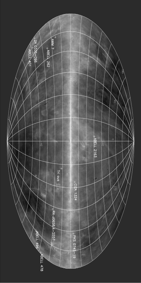
shows the location of each of the clusters in our sample superimposed upon the all sky map of the 100 $\mu$m emission observed by IRAS. The IRAS map is a good tracer of dust in the galaxy, and shows that the clusters in our sample that do not lie in the galactic plane are still located in areas with high $n_{\rm H}$. Figure 2 also shows that our clusters sample a wide range of galactic sight lines.

2.2. Data Reduction

We extracted spectra from the pn and two MOS CCD detectors that comprise the EPIC camera on XMM-Newton. These detectors’ moderate resolution of $\Delta E\sim 50--100$ eV and large field of view (30 arcminute diameter) are well matched to our requirements. The cluster data were re-extracted from the raw ODF files using SAS version 5.4.1. After filtering to eliminate periods with high background rates, we choose regions on the CCDs that encompass most of a cluster’s emission without a significant contribution from the background. This was done by selecting by eye a circular region centered on the cluster with a radius extending to where the cluster emission drops to about three times the background level. Backgrounds were local, and taken from areas in the field of view without cluster emission. Ancillary response files and response matrices are generated using arfgen and rmfgen within SAS.

We extracted spectra between 0.46–10.0 keV in the MOS1 and MOS2 detectors, and between 0.46–7.2 keV in the pn in order to avoid large background lines above 7.2 keV in the pn. Our lower energy cutoff is 0.46 keV in order to avoid problems with the calibration of the redistribution function at very low energies.

2.3. Extra Edge

In order to obtain the greatest signal to background ratio we would like to fit the data from all three CCD detectors on XMM-Newton. However, early on we discovered that oxygen absorption results from the three detectors did not agree. For some clusters, when the MOS detectors showed substantial absorption the pn detector showed almost none. We examined data from an XMM-Newton observation of the bright quasar 3C 273 (a good continuum source at the energies of interest) in order to investigate this effect at low galactic columns (3C 273 has $n_{\rm H}$ = $1.8\times 10^{20}\,\mbox{cm}^{-2}$). We found that there are substantial residuals in the MOS detectors at the location of the oxygen edge. Figure 3

Figure 3.— A spectral fit to the bright quasar 3C 273 with the 3 CCD detectors of the EPIC camera on XMM-Newton. The residuals above the oxygen edge at 544 eV show the large discrepancy between detectors; the higher resolution data from the pn detector is well fit throughout the band, while the MOS data have significant residuals. We address this problem by including an extra edge to the model that is discussed in section §2.3.

shows the residuals to the 3C 273 fit at the location of the oxygen edge and illustrates the large deviation in the MOS detectors. We also observe this effect towards the Coma cluster, another low galactic column source ($n_{\rm H}$ = $9.2\times 10^{19}\,\mbox{cm}^{-2}$).

We interpret this effect as an inaccuracy in the response matrices for the MOS detectors. Such an effect could possibly be caused by the outgassing of organic materials onto the surface of the MOS detectors, and is seen in observations taken with both the thin and medium filters. The oxygen edge in the detector is caused by molecular compounds of oxygen, and its energy of 0.53 keV is slightly offset from the ISM atomic edge at 0.542 keV. However, the correct determination of this instrumental feature could effect measurements of the ISM oxygen abundance at low column densities. Figure 4 shows the magnitude of the instrument edge in the MOS detectors.

Figure 4.— The instrumental response of the detectors of the EPIC camera in the region of the oxygen edge. The upper trace is the pn detector, and the lower two traces are the MOS detectors. The optical depth of the MOS instrumental edge is $\tau=0.72$. The different shape in the edge structure of the front-side illuminated MOS and back-side illuminated pn is clearly seen.

We compensate for this problem by introducing an extra edge into the fit at the solid state oxygen K-shell energy of 0.53 keV. When the extra edge component has optical depths of 0.22 for the MOS1 and 0.20 for the MOS2 the fitted oxygen absorption is consistent between all three detectors for 3C 273 and Coma, so we use these values for our cluster fits.

This problem has been brought to the attention of the XMM-Newton EPIC instrument team. They have kindly supplied a beta version of a revised quantum efficiency file that is meant to address this problem. The tests we have made using this file have provided results that are consistent with the extra edge method described above.

2.4. Spectral Fitting

We use XSPEC version 11.3.0 to fit the data. The cluster emission is modeled by the apec (v. 1.3.1) plasma code (Smith et al., 2001), and the intervening galactic material by the tbvarabs model (Wilms et al., 2000) (XSPEC model: edge * tbvarabs * apec; the edge component of the model is discussed in §2.3).

The tbvarabs model models the absorption due to photoionization from the abundant elements up to nickel. It also takes into account absorption from molecular hydrogen and depletion of the elements onto grains. The abundance of each of the elements can be individually fit, as well as the depletion fraction. The model elemental abundances are computed from the observables (e.g., spectral line equivalent width, optical depth) by specifying a table of solar elemental abundances selectable by the user. We choose the compilation of theoretical X-ray absorption cross sections by Verner et al. (1996), and the solar abundances of Wilms et al. (2000). Although Lodders (2003) has published a more recent compilation, we feel that her solar abundance for helium that takes into account heavy element settling in the sun results in an abundance that is too low for good ISM modeling. Her compilation of recent results for carbon, nitrogen, and oxygen needs to be taken into account and is very similar to the Wilms et al. model abundances that we use.

For our investigation, the dominant contributors to galactic absorption are hydrogen, helium, and oxygen. Secondary contributors observable in the XMM-Newton band are neon and iron (from the L-shell). We initially set the hydrogen column to the galactic 21 cm value from Dickey & Lockman (1990), but allow it to vary with the fit. The helium abundance is not well constrained independently of the hydrogen value, and is set to solar in our fit. Neon and iron are also initially set to their solar abundance values, but are allowed to vary with the fit. All other elements are fixed to their solar abundance values as determined by Wilms et al. (2000). The grain and depletion parameters are set to their default value in the tbvarabs model, but these parameters do not significantly affect the results of our fitting. All of the parameters in the tbvarabs portion of the model are constrained to have the same value for each of the three EPIC detectors.

Initial values for the cluster temperature, metal abundance, and redshift are given in Table 1, taken from the work of Horner (2001). The cluster temperature and metal abundance are constrained to have the same value for the three EPIC detectors, but the cluster redshift is allowed to vary separately in each detector in order to compensate for any small energy calibration errors in the data.

The clusters Abell 478 and Abell 262 had high $\chi^{2}$ values compared to the other clusters when fit with one temperature plasma models. This is a result of a lower temperature cooling flow component in the cluster contributing flux at lower energies and causing the model to underestimate the galactic hydrogen and oxygen absorption. Kaastra et al. (2004) show that Abell 262 is more successfully fit with a two temperature model using the same XMM-Newton observations that we have extracted from the archives for this paper, and Sakelliou & Ponman (2004) also require a two temperature model for Abell 478. For these clusters, we use a two component thermal model with galactic absorption and an extra edge, [edge*tbvarabs*(apec + apec)] and quote the temperature of the higher temperature component representing the main cluster emission in Table 2. The metal abundance of the second thermal component was tied to that of the first component and the normalization left free.

A spectrum with residuals to the fit for a typical cluster is given in Figure 5.

Figure 5.— Fits to the cluster PKS 0745-19. The data are shown with errors and the model is a solid line in the top plot of each panel. The residuals are shown in the bottom plot of each panel. The top panel shows that the overall fit is good to a model that includes an extra edge component in the MOS detectors, as is the .5 keV region where the oxygen signal lies. The biggest residual is at 1 keV and is from iron L-shell emission, and does not affect the oxygen fit. In the bottom panel, the data was first fit with the standard model. Then, the model oxygen abundance was set to zero to illustrate the strength and importance of the galactic oxygen absorption component.

In the top panel we show the spectrum fit with the model, while in the bottom panel we set the galactic oxygen abundance to zero to illustrate the strength of the absorption signal.

3. Results

Table 2X-ray Determined Galactic Absorption towards Galaxy Clusters

Cluster	$z$	$kT$	Z	$n_{\rm H}$	Oxygen	Counts	$\chi^{2}$	dof
		[keV]			abundance		per dof
PKS 0745-19	0.100	7.173	0.68	5.620${}_{5.350}^{5.930}$	0.74${}_{0.59}^{0.88}$	3.7e+05	1.09	2121
ABELL 0401	0.069	8.738	0.58	1.050${}_{0.990}^{1.080}$	0.56${}_{0.40}^{0.79}$	2.8e+05	1.06	1918
Tri aus	0.050	10.144	0.57	1.500${}_{1.430}^{1.570}$	1.02${}_{0.86}^{1.21}$	4.2e+05	1.05	2202
AWM7	0.016	3.652	1.14	1.140${}_{1.130}^{1.160}$	0.95${}_{0.92}^{1.02}$	1.4e+06	1.25	2362
ABELL 0478	0.081	6.588	0.66	3.640${}_{3.630}^{3.660}$	1.03${}_{1.01}^{1.06}$	1.9e+06	1.39	2348
RX J0658.4-5557	0.297	12.392	0.44	0.310${}_{0.250}^{0.370}$	0.48${}_{0.00}^{1.15}$	1.5e+05	0.99	1474
ABELL 2163	0.194	12.997	0.40	2.130${}_{2.000}^{2.290}$	0.97${}_{0.74}^{1.21}$	1.1e+05	1.02	1428
ABELL 0262	0.014	2.057	0.78	0.850${}_{0.790}^{0.900}$	0.70${}_{0.43}^{0.85}$	4.4e+05	1.26	1727
2A 0335+096	0.034	2.661	0.98	3.160${}_{2.960}^{3.350}$	0.82${}_{0.69}^{1.10}$	5.8e+04	1.18	936
ABELL 0496	0.031	3.556	0.96	0.640${}_{0.620}^{0.660}$	0.76${}_{0.68}^{0.86}$	5.8e+05	1.29	2059
CIZA 1324	0.018	2.944	0.94	5.750${}_{5.180}^{6.500}$	1.32${}_{0.95}^{1.73}$	8.8e+04	1.09	1220

Note. — All values are from the X-ray fit to the XMM-Newton data. Values in sub and superscript are the range of the 90% confidence interval.

The results from the X-ray spectral fits are shown in Table 2.

Column 1 gives the cluster name, while columns 2–4 give the fitted cluster redshift, temperature, overall metal abundance, and hydrogen column. We give the results for the observed X-ray column of galactic hydrogen in column 5 of the table. The main results are for the elemental abundance of galactic oxygen along the line of site towards the background cluster and are given in column 6. Columns 7, 8, and 9 of the table are meant to illustrate the quality of the fit and list the number of photons in the X-ray spectrum from all three EPIC detectors, the reduced $\chi^{2}$, and the number of degrees of freedom of the fit.

3.1. Hydrogen

The total galactic hydrogen column density is composed of several parts: the neutral atomic gas measured by 21 cm radio observations; the warm, ionized H II gas that is sometimes associated with H$\alpha$ emission; and molecular hydrogen, H₂, often associated with CO emission. The X-ray measure of the hydrogen column, $n_{{\rm H}_{X}}$, is sensitive to all these forms and is indicative of the total hydrogen column.

The X-ray total column is also sensitive to the helium component along the line of sight. At the X-ray energies of these observations, the absorption cross section due to helium is substantial and is greater than the hydrogen component. However, the helium is mostly primordial in origin and the hydrogen to helium ratio in the galaxy is assumed to be uniform. Therefore, variations in the helium abundance or distribution are not expected to have a significant effect on the total hydrogen columns.

Figure 6

Figure 6.— The X-ray total hydrogen column density plotted against the neutral hydrogen value derived from the 21  cm observations in Dickey & Lockman (1990). The hydrogen columns are in units of $10^{21}$ cm^-2. Many clusters have error bars smaller than the plotted points. The X-ray values are generally higher because these observations are sensitive to all forms of hydrogen and detect H₂ that could not be seen with the 21 cm observations. The molecular component of $n_{\rm H}$ becomes most important above columns of $\sim 0.5\times 10^{21}$ cm^-2 where the H₂ is sufficiently dense enough to shield itself from dissociating radiation from hot young galactic stars.

shows the X-ray determined total hydrogen column from this work plotted against the column of neutral hydrogen measured by the 21 cm observations of Dickey & Lockman (1990). The X-ray measure of the hydrogen column is well correlated with the 21 cm observations, as well as with the optical reddening $E_{B-V}$ determined by IRAS (Schlegel et al., 1998) as shown in Figure 7.

Figure 7.— The correlation of $n_{\rm H}$ derived from X-ray observations with other measures of the ISM towards the lines of sight of the 11 clusters in our sample. The top left panel shows $n_{{\rm H}_{X}}$ against the 21 cm radio observation of neutral atomic hydrogen [the data are in units of $10^{21}$ cm^-2]; the top right panel shows shows $n_{{\rm H}_{X}}$ against the $B$-band optical extinction data in magnitudes; the lower left panel shoes $n_{{\rm H}_{X}}$ against the optical reddening; and the lower right panel shoes $n_{{\rm H}_{X}}$ against the IRAS DIRBE corrected $100\mu$m emission in MJy sr^-1. The X-ray emission is better correlated with the reddening and IRAS emission which are also sensitive to the effects of dust and molecular clouds.

The direct comparison of the X-ray and 21 cm derived columns in Figure 6 shows that the X-ray columns are in general higher than the 21 cm ones. Arabadjis & Bregman (1999) (AB) showed that below columns of approximately $0.5\times 10^{21}$ cm^-2 the X-ray derived $n_{\rm H}$ column closely matches the 21 cm value, suggesting that neutral atomic hydrogen can account for all of the observed column below these densities. However, above $0.5\times 10^{21}$ cm^-2, the X-ray column exceeds the 21 cm column and the contribution from other hydrogen sources such as molecular hydrogen become important. This effect can most easily be seen by plotting the ratio of the X-ray to 21 cm column as a function of the X-ray column, as we do with our data in Figure 8.

Figure 8.— The overabundance of the X-ray derived $n_{\rm H}$ compared to the 21 cm derived value [in units of $10^{21}$ cm^-2].

While many of our clusters are in the AB list, the better spectral resolution, broader bandpass, and higher signal to noise data of our XMM-Newton observations are better able to characterize the thermal emission of the underlying cluster. In Figure 9

Figure 9.— A comparison of the Arabadjis & Bregman (1999) X-ray derived $n_{\rm H}$ values to those in this study [in units of $10^{21}$ cm^-1].

we plot our derived X-ray columns against those of AB and find that they are in good agreement.

Figure 8 indicates that above columns of $0.5\times 10^{21}$ cm^-2 the total hydrogen column cannot be accounted for solely by neutral atomic hydrogen and that other contributors must be taken into account. These contributors include ionized hydrogen, H II, and molecular hydrogen, H₂, discussed in the sections below.

It is also possible that for high columns the 21 cm derived $n_{\rm H}$ values are incorrect because they assume that the neutral atomic hydrogen is optically thin. At higher columns, the gas becomes sufficiently optically thick to undergo self shielding and self-absorption. Strasser & Taylor (2004) have conducted an emission-absorption study of H I in the galactic plane which measures this effect. They have found that the 21 cm columns derived from emission alone (such as Dickey & Lockman (1990)) require only a $\sim$2% correction at columns of $1.0\times 10^{21}$ cm^-2 in order to arrive at the actual galactic hydrogen column. This correction is less than the statistical error of our X-ray fits and so we ignore it.

3.1.1 Ionized Hydrogen

The contribution of ionized H II to the total column $n_{\rm H}$ is small. Though X-ray photoionization absorption from the ionized hydrogen is itself not possible, some small amount of absorption from the associated metals in H II regions is possible.

AB noted in their study that below columns of $0.5\times 10^{21}$ cm^-2 the X-ray total column can be completely explained solely by contributions from neutral atomic hydrogen as measured by 21 cm observations. Laor et al. (1997) observed the X-ray spectra of AGN and came to a similar conclusion. Attempts to constrain H II using IRAS 100 $\mu$m data by Boulanger et al. (1996) have also led to low values for H II, with Kuntz (2001) suggesting that less than 20% of the IRAS emission can be associated with H II.

Recently, the WHAM project has measured H II emission by observing at H$\alpha$ (Haffner et al., 2003). They also find that H II is not a significant contributor to $n_{\rm H}$.

3.1.2 Molecular Hydrogen and CO Measurements

CO emission in the radio is known to be correlated with concentrations of molecular hydrogen. The correlation is sufficient that a constant coefficient can be used to estimate the amount of H₂ present from the measured CO emission. Although the correspondence does not hold exactly for all densities, (there is significant diffuse H₂ at high galactic latitudes found without substantial CO emission), a linear correlation H₂ = X CO is found at densities high enough for the H₂ to shield the CO from radiation-induced dissociation. The value of this so-called X factor is somewhat controversial and is thought to vary somewhat depending on the local environment. However, Dame et al. (2001) have measured CO emission across the entire galactic plane and have derived an overall X factor of $1.8\times 10^{20}$ K^-1km^-1s cm^-2.

These CO measurements and the X factor can be used to provide a measure of the molecular hydrogen content along our lines of sight. This information can be combined with the X-ray and 21 cm derived hydrogen column densities in order to diagnose the hydrogen composition. The X-ray derived $n_{{\rm H}_{X}}$ measures the total column of hydrogen in all forms, while the 21 cm column measures the dominant neutral atomic component. The CO measurements can then be used to constrain the proportion of the remaining component that is molecular hydrogen.

PKS 0745-19 and CIZA 1324 are the only clusters in our sample that have spatial coordinates that place them within the bounds of the Dame et al. CO galactic plane survey. We have extracted CO fluxes of 4.46 and 1.72 K km s^-1 for these lines of sight, which can be associated with molecular hydrogen columns ($n_{H_{2}}$) of $8.02\times 10^{20}$ cm^-2 and $3.09\times 10^{20}$ cm^-2 using the X factor from Dame et al.. Equivalent hydrogen columns of $n_{\rm H}$ = $2.29\times 10^{21}$ cm^-2 and $8.81\times 10^{20}$ cm^-2 are computed using a factor 2.85 for the conversion of H₂ to $n_{\rm H}$ as recommended by Wilms et al. (2000).

Table 3Hydrogen Column Decomposition

	PKS 0745-19	CIZA 1324
	[$10^{21}$ cm-2]	[$10^{21}$ cm-2]
$n_{\rm H}$ (21 cm)	4.24	3.81
$n_{H_{2}}$ (CO)	0.802	0.309
equivalent $n_{\rm H}$ (CO)	2.29	0.881
$n_{\rm H}$ (21 cm + CO)	$6.53_{5.9}^{7.2}$	$4.69_{4.2}^{5.2}$
$n_{\rm H}$ (X-ray)	$5.6^{5.9}_{5.4}$	$5.8_{5.2}^{6.5}$

Table 3 shows the breakdown of the total hydrogen column into its components for the two lines of sight towards PKS 0745-19 and CIZA 1324. The fourth row shows the sum of the 21 cm neutral hydrogen component and the CO derived molecular component, and the fifth row shows the total column derived from the X-ray observations. The errors on the $n_{\rm H}$(21 cm + CO) values come from assuming a 10% error. Arabadjis & Bregman (1999) show that the error on the 21 cm data is approximately 5%; when combined with the uncertainty in the CO data and the CO to H₂ conversion 10% is a plausible value. The error in the $n_{{\rm H}_{X}}$ value is the 90% confidence interval from the X-ray fit.

The results from these two lines of sight show that the $n_{\rm H}$(21 cm + CO) and $n_{{\rm H}_{X}}$ values are in fair agreement within the 90% confidence regions.

Other evidence supports our claim that the excess absorption in the X-ray hydrogen column can be ascribed to H₂. Federman et al. (1979) show that at the columns where we begin to see $n_{{\rm H}_{X}}$ larger than those measured by 21 cm measurements, H₂ is dense enough to start shielding itself from incident ionizing radiation that dissociates it at lower densities. Also, the Copernicus satellite has found that these are the columns at which H₂ starts to become abundant (Savage et al., 1977).

3.2. Galactic Oxygen Abundance

The main result from this work is the X-ray measurement of the galactic oxygen abundance. Column 6 of Table 2 gives our results for the abundance of oxygen using the best fit galactic absorption model. These results are plotted against the X-ray $n_{\rm H}$ from column 5 in Figure 10.

Figure 10.— The galactic oxygen abundance plotted against the X-ray hydrogen column for 11 lines of sight towards galaxy clusters. The abundances are given with respect to the solar value in Wilms et al. (2000), and the hydrogen columns are in units of $10^{21}$ cm^-2. The best fit value for the oxygen abundance is O/H $=0.99\pm 0.06$ solar.

The galactic oxygen abundance is uniform for all our lines of sight and is centered on the solar value. The best fit value is O/H = 0.99 with a standard deviation of 0.06. Figure 10 shows that there is no trend in the oxygen abundance with increasing hydrogen column, and that a single value for the oxygen abundance is a reasonable fit to the individual data points. These results stand in contrast to many years of work on metal depletion in the ISM and support the recent compilation by Jenkins (2004) that shows that oxygen has little depletion in our galaxy.

3.3. Oxygen Abundance Variations

The eleven lines of sight towards the clusters in this study traverse many different galactic environments. A diagnostic of the different regions probed by these sightlines is the ratio of 21 cm $n_{\rm H}$ to $n_{{\rm H}_{X}}$ that can be used to investigate the density of the observed oxygen. It is possible that the lines of sight passing through higher density regions could have different oxygen abundances because of their proximity to molecular clouds and star forming regions.

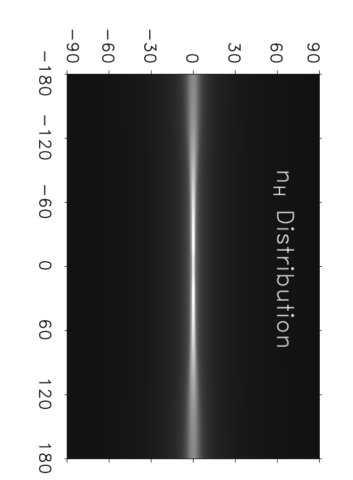
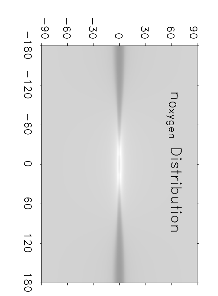
In order to try and observe this effect and separate it from the a priori expected abundance variations caused by the galactic abundance gradient and galactic hydrogen distribution, we use the Milky Way mass models of Wolfire et al. (2003) and the measurements of the spatial gradient of the oxygen abundance measured in planetary nebulae by Henry et al. (2004). Our approach is to take the Wolfire et al. density model for galactic neutral hydrogen, multiply it by the oxygen abundance in Henry et al. (taking into account the spatial gradient across the galaxy) and integrate outward from the Sun to determine the total hydrogen and oxygen columns. We generate a simple 360 by 180 pixel sky map with pixels spaced every degree in latitude and longitude. The resulting map indicates the variation of the hydrogen and oxygen columns across the sky given our simple model, even though the pixel spacing and map projection emphasize regions at high latitudes.

The Wolfire et al. model for neutral hydrogen has an exponential falloff with galactic radius for large radii, and a Gaussian distribution in the height above the disk. Also, the center of the galaxy is low in atomic hydrogen, and Wolfire et al. exclude hydrogen from the central part of the galaxy:

$$\Sigma_{\mbox{{H~{}I}}}(R)=\left\{\begin{array}[]{lcclc}1.4R_{k}-0.6&(3&\leq&R_{k}<&4)\\ 5&(4&\leq&R_{k}<&8.5)\\ 6.12\left(R_{k}/8.5\right)-1.12{}{}&(8.5&\leq&R_{k}<&13)\\ 8.24\,{e}^{-\left(R_{k}-13\right)/4}&(13&\leq&R_{k}<&24)\end{array}\right.$$

where $\Sigma_{\mbox{{H~{}I}}}(R)$ is the H I surface density in $M_{\odot}$ pc^-2, $R_{k}\equiv R/(1$ kpc), and where we use the conversion 1 $M_{\odot}$ pc${}^{-2}=1.25\times 10^{20}$ H I cm^-2.

The Henry et al. spatial oxygen abundance gradient has the logarithmic abundance going linearly as the galacto-centric radius:

$$\mbox{O/H}(r)=10^{(8.97-0.037r)-12.0},$$

where O/H($r$) is the abundance of oxygen by number with respect to hydrogen as a function of the galactic radius $r$ in kpc. The Henry et al. results are normalized to the solar oxygen abundance given in Allende Prieto et al. (2001) and measure oxygen abundances in planetary nebulae. These PN abundances are consistent with measurements made in H II regions by Deharveng et al. (2000).

Figure 11 shows the hydrogen column across the sky, the oxygen abundance, and a scatterplot of the oxygen abundance versus the hydrogen column for sightlines across the entire sky. This figure shows that we should expect the hydrogen column and oxygen abundance to be very uniform across most of the sky, except for the region within a few degrees of the galactic plane. This is in agreement with the oxygen results shown in Figure 10.

Figure 11.— The distribution of $n_{\rm H}$ and oxygen on the sky as computed by integrating along all lines of sight through a model of the galaxy. The first panel shows the integrated neutral hydrogen column density integrated from the solar position through the galactic density model given by Wolfire et al. (2003), the second panel shows the oxygen abundance derived by incorporating the Henry et al. (2004) oxygen gradient into the hydrogen model, and the third panel is a scatterplot of the oxygen abundance against the hydrogen column for each location in the skymaps. The lines in the third panel are lines of constant galactic latitude, with the low latitudes on the right. The oxygen abundance is very uniform across most of the sky, but shows some variation within two degrees of the galactic plane.

3.3.1 Spatial Consistency of the Oxygen Abundance

In order to look for differences in the oxygen abundance related to galactic environment, we plot the oxygen abundance against the ratio of the X-ray to 21 cm $n_{\rm H}$ in Figure 12.

Figure 12.— A plot showing the constancy of the ISM oxygen abundance with respect to different overdensities of $n_{{\rm H}_{X}}$. If the high column density lines of sight can be associated with denser molecular clouds, this result indicates that the relative abundance of oxygen in these clouds is not different from its value in other parts of the galaxy.

The ratio of the X-ray to 21 cm derived $n_{\rm H}$ stands in for density: we expect that any hydrogen seen in the X-ray but not in the radio is most likely molecular and found in denser clouds. If the denser regions have a different oxygen abundance than the more diffuse regions, we would expect a trend in the plot. However, when the left most point with the large error bars is ignored (RX J0658), Figure 12 indicates that the oxygen abundance shows no trend with the X-ray to 21 cm $n_{\rm H}$ ratio, and that the galactic oxygen abundance is the same in all regions measured. This disagrees with the STIS observations reported in Cartledge et al. (2001), but agrees with the more recent FUSE data of Jensen et al. (2003). X-ray observations towards galactic star forming regions also indicate that these denser parts of the ISM have abundances similar to those of the local diffuse ISM (Vuong et al., 2003).

4. Systematic Errors

The sytematic errors outweigh the statistical errors in our measurements. The main contributors to the systematic error include the correct determination of the extra edge component in the spectral fits and the galactic helium abundance.

4.1. Error in the Extra Edge Determination

In §2.3 we measured the size of the extra edge necessary to reconcile the MOS and pn oxygen abundances by looking at high signal to noise data from the bright sources 3C 273 and the Coma cluster and added an extra edge component at oxygen to the MOS fits so that they would match the pn.

It is possible that this method does not completely reconcile the MOS and pn derived abundances for all epochs. If the magnitude of the extra edge component is changing with time (e.g., if there is a progressive buildup of a contaminant in the camera), then we can expect that the extra edge determined from the calibration sources will not accurately reflect the value necessary for each of the cluster observations, which are taken at several different epochs. We checked for temporal variations in the extra edge component derived from 3C273 observations at several epochs but did not find a significant difference in the data taken at different times. There still could be a small time dependent component of the extra edge, but we argue more generally in the following paragraphs that the uncertainty in the extra edge component does not have a significant effect on the measured abundances.

Figure 13

Figure 13.— A comparison of results fit with and without the extra oxygen edge model component. The first panel shows the results of fitting a model with the extra edge component set to zero. In general, the derived oxygen abundances for the data points with the smallest errors are higher than the fits that include the extra edge (panel 2) because the fit compensates for the extra absorption missing from the instrumental response matrix. The third panel shows the oxygen abundances derived from fits using only data from the pn detector in order to avoid the problems with the MOS detectors. The models fit to this data give similar results to the models with the extra edge and indicate that the inclusion of the extra edge in the model is necessary.

shows two different ways to check this potential problem. The first panel of Figure 13 shows the ISM oxygen abundances that result from fitting with the magnitude of the extra edge component set to zero. Also, the third panel of Figure 13 shows the oxygen abundances found from fitting to only the pn data, which does not require the extra edge component.

We expect that fits without the extra edge in the model will produce higher ISM oxygen abundances. Panel one does show that the oxygen abundances are generally higher without the extra edge than the normal fits in panel two.

We would also expect the oxygen abundances found from fitting only to the pn data to be lower than those found with all three detectors and the extra edge component in the MOS set to zero. In fact, although the abundances derived from the pn alone in panel three are slightly lower than abundances with the extra edge in panel two, the difference is small. The main difference is between the data sets fit with and without the extra edge component (panels one and two). This significant difference, and the fact that the models with the edge match the pn alone models, indicate that the presence of an extra edge component is necessary for a proper fit and gives good results.

4.2. Helium Abundance Errors

Below the oxygen edge at 542 eV, the absorption due to helium in the ISM dominates the absorption from all other elements. Above this energy oxygen dominates the ISM absorption, but the helium component is still much larger than the hydrogen absorption which is falling off rapidly approximately as $E^{-3}$. The galactic helium abundance is somewhat uncertain, and errors in this value could affect our abundance measurements because of its strong contribution to the ISM X-ray absorption at our energies of interest. If the helium abundance in our model is too low, the hydrogen component will be increased to compensate. This will affect the oxygen abundance, since it is measured with respect to the hydrogen component. If the adopted helium abundance is too high, a similar result occurs, but in the opposite direction.

We have investigated this effect by fitting our data with two different helium abundances. The first data set is fit with the standard wilm abundances in XSPEC, and the second set is fit with the helium abundance frozen at 80% of the wilm value. This value was chosen because it is representative of the differences between current helium abundance determinations: The wilm helium abundance is $9.77\times 10^{-2}$ by number with respect to hydrogen, and the helium abundance of lodd is $7.92\times 10^{-2}$, about a 20% difference.

Figure 14

Figure 14.— A demonstration of the effect of an uncertain helium abundance on oxygen abundance results. The circular points result from a fit to the data using the solar abundances of Wilms et al. (2000). The stars are fit using a helium abundance of 80% of the wilm value, as explained in the text. As expected, the lower solar helium abundance drives up the derived value of $n_{\rm H}$  which in turn reduces the normalized oxygen abundance. The effect is noticeable, but smaller than the errors on the fits (shown in Figure 10).

shows the results from these fits. The points plotted as circles (with the cluster name attached) are from the canonical wilm fit, and the stars are from the low helium fit. As expected, the lower helium abundance raises the hydrogen abundance found in the fit and lowers the oxygen abundance. However, the effect on the the oxygen abundance is smaller than the scatter between the multiple cluster observations.

5. Summary

We have used X-ray observations of galaxy clusters to measure the oxygen abundance and total hydrogen column of the ISM. Our measurements of galactic absorption have shown that the X-ray column, $n_{{\rm H}_{X}}$, is in close agreement with the 21 cm value for neutral hydrogen for columns less than approximately $0.5\times 10^{21}\mbox{cm}^{-2}$. Above $0.5\times 10^{21}\mbox{cm}^{-2}$, the X-ray column is much higher than the 21 cm value by up to a factor of 2.5. This result indicates that there is substantial absorption at high columns in addition to that provided by neutral hydrogen, and is most likely from clouds of molecular hydrogen. Measurements of the contribution to $n_{{\rm H}_{X}}$ from H₂ derived from CO observations show that the molecular hydrogen column density makes up for the observed difference.

We also measure the ISM oxygen abundance by observing the K-shell photoionization edge at 542 eV. After taking into account calibration problems in the EPIC MOS detectors on XMM-Newton, we find that the galactic oxygen abundance is consistent with the most recent solar values. Previously, oxygen abundance measurements have suggested that oxygen is depleted in the ISM because gas phase measurements have shown the abundance to be lower than the adopted solar value. However, the accepted solar value has recently decreased as a result of better modeling of solar spectra (Asplund et al., 2004). Our measurement in conjunction with the recent solar value shows that oxygen is not depleted in the ISM, in agreement with Jenkins (2004). We also find that the oxygen abundance is uniform across an order of magnitude in $n_{{\rm H}_{X}}$, suggesting similar compositions for higher density regions in the ISM and more diffuse regions, in agreement with the conclusions of Vuong et al. (2003).

References

- Anders & Grevesse (1989) Anders, E. & Grevesse, N. 1989, Geochim. Cosmochim. Acta, 53, 197
- Allende Prieto et al. (2001) Allende Prieto, C., Lambert, D. L., & Asplund, M. 2001, ApJ, 556, L63
- André et al. (2003) André, M. K. et al. 2003, ApJ, 591, 1000
- Arabadjis & Bregman (1999) Arabadjis, J. S. & Bregman, J. N. 1999, ApJ, 510, 806
- Asplund et al. (2004) Asplund, M., Grevesse, N., Sauval, A. J., Allende Prieto, C., & Kiselman, D. 2004, A&A, 417, 751
- Boulanger et al. (1996) Boulanger, F., Abergel, A., Bernard, J.-P., Burton, W. B., Desert, F.-X., Hartmann, D., Lagache, G., & Puget, J.-L. 1996, A&A, 312, 256
- Burstein & Heiles (1982) Burstein, D. & Heiles, C. 1982, AJ, 87, 1165
- Cardelli et al. (1994) Cardelli, J. A., Sofia, U. J., Savage, B. D., Keenan, F. P., & Dufton, P. L. 1994, ApJ, 420, L29
- Cardelli et al. (1996) Cardelli, J. A., Meyer, D. M., Jura, M., & Savage, B. D. 1996, ApJ, 467, 334
- Cartledge et al. (2001) Cartledge, S. I. B., Meyer, D. M., Lauroesch, J. T., & Sofia, U. J. 2001, ApJ, 562, 394
- de Plaa et al. (2004) de Plaa, J., Kaastra, J. S., Tamura, T., Pointecouteau, E., Mendez, M., & Peterson, J. R. 2004, A&A, 423, 49
- de Vries et al. (2003) de Vries, C. P., den Herder, J. W., Kaastra, J. S., Paerels, F. B., den Boggende, A. J., & Rasmussen, A. P. 2003, A&A, 404, 959
- Crinklaw et al. (1994) Crinklaw, G., Federman, S. R., & Joseph, C. L. 1994, ApJ, 424, 748
- Dame et al. (2001) Dame, T. M., Hartmann, D., & Thaddeus, P. 2001, ApJ, 547, 792
- Deharveng et al. (2000) Deharveng, L., Peña, M., Caplan, J., & Costero, R. 2000, MNRAS, 311, 329
- Dickey & Lockman (1990) Dickey, J. M. & Lockman, F. J. 1990, ARA&A, 28, 215
- Draine (2004) Draine, B. T. 2004, Origin and Evolution of the Elements, 320
- Federman et al. (1979) Federman, S. R., Glassgold, A. E., & Kwan, J. 1979, ApJ, 227, 466
- Fitzpatrick (1996) Fitzpatrick, E. L. 1996, ApJ, 473, L55
- Grevesse & Sauval (1998) Grevesse, N. & Sauval, A. J. 1998, Space Science Reviews, 85, 161
- Grevesse & Sauval (1999) Grevesse, N. & Sauval, A. J. 1999, A&A, 347, 348
- Haffner et al. (2003) Haffner, L. M., Reynolds, R. J., Tufte, S. L., Madsen, G. J., Jaehnig, K. P., & Percival, J. W. 2003, ApJS, 149, 405
- Henry et al. (2004) Henry, R. B. C., Kwitter, K. B., & Balick, B. 2004, AJ, 127, 2284
- Holweger (2001) Holweger, H. 2001, AIP Conf. Proc. 598: Joint SOHO/ACE workshop ”Solar and Galactic Composition”, 598, 23
- Horner (2001) Horner, D. 2001, Ph.D. Dissertation, Department of Astronomy, University of Maryland College Park
- Horner et al. (ApJS submitted) Horner, D. J., Baumgartner, W. H., Gendreau, K. C., & Mushotzky, R. F. 2004, ApJS, submitted
- Jenkins (1987) Jenkins, E. B. 1987, ASSL Vol. 134: Interstellar Processes, 533
- Jenkins (2004) Jenkins, E. B. 2004, Origin and Evolution of the Elements, 339
- Jensen et al. (2003) Jensen, A. G., Rachford, B. L., & Snow, T. P. 2003, American Astronomical Society Meeting, 203,
- Juett et al. (2004) Juett, A. M., Schulz, N. S., & Chakrabarty, D. 2004, ApJ, 612, 308
- Kaastra et al. (2004) Kaastra, J. S., et al. 2004, A&A, 413, 415
- Kuntz (2001) Kuntz, K. D. 2001, Ph.D. Thesis, Department of Astronomy, University of Maryland College Park
- Laor et al. (1997) Laor, A., Fiore, F., Elvis, M., Wilkes, B. J., & McDowell, J. C. 1997, ApJ, 477, 93
- Lodders (2003) Lodders, K. 2003, ApJ, 591, 1220
- Mathis (1996) Mathis, J. S. 1996, ApJ, 472, 643
- Meyer et al. (1994) Meyer, D. M., Jura, M., Hawkins, I., & Cardelli, J. A. 1994, ApJ, 437, L59
- Moos et al. (2002) Moos, H. W. et al. 2002, ApJS, 140, 3
- Oliveira et al. (2003) Oliveira, C. M., Hébrard, G., Howk, J. C., Kruk, J. W., Chayer, P., & Moos, H. W. 2003, ApJ, 587, 235
- Paerels et al. (2001) Paerels, F. et al. 2001, ApJ, 546, 338
- Page et al. (2003) Page, M. J., Soria, R., Wu, K., Mason, K. O., Cordova, F. A., & Priedhorsky, W. C. 2003, MNRAS, 345, 639
- Pilyugin et al. (2003) Pilyugin, L. S., Ferrini, F., & Shkvarun, R. V. 2003, A&A, 401, 557
- Sakelliou & Ponman (2004) Sakelliou, I., & Ponman, T. J. 2004, MNRAS, 351, 1439
- Savage & Sembach (1996) Savage, B. D., & Sembach, K. R. 1996, ARA&A, 34, 279
- Schlegel et al. (1998) Schlegel, D. J., Finkbeiner, D. P., & Davis, M. 1998, ApJ, 500, 525
- Savage et al. (1977) Savage, B. D., Drake, J. F., Budich, W., & Bohlin, R. C. 1977, ApJ, 216, 291
- Smith et al. (2001) Smith, R. K., Brickhouse, N. S., Liedahl, D. A., & Raymond, J. C. 2001, ApJ, 556, L91
- Sofia & Meyer (2001) Sofia, U. J. & Meyer, D. M. 2001, ApJ, 554, L221
- Strasser & Taylor (2004) Strasser, S. & Taylor, A. R. 2004, ApJ, 603, 560
- Verner et al. (1996) Verner, D. A., Ferland, G. J., Korista, K. T., & Yakovlev, D. G. 1996, ApJ, 465, 487
- Vuong et al. (2003) Vuong, M. H., Montmerle, T., Grosso, N., Feigelson, E. D., Verstraete, L., & Ozawa, H. 2003, A&A, 408, 581
- Weisskopf et al. (2004) Weisskopf, M. C., O’Dell, S. L., Paerels, F., Elsner, R. F., Becker, W., Tennant, A. F., & Swartz, D. A. 2004, ApJ, 601, 1050
- Willingale et al. (2001) Willingale, R., Aschenbach, B., Griffiths, R. G., Sembay, S., Warwick, R. S., Becker, W., Abbey, A. F., & Bonnet-Bidaud, J.-M. 2001, A&A, 365, L212
- Wilms et al. (2000) Wilms, J., Allen, A., & McCray, R. 2000, ApJ, 542, 914
- Wolfire et al. (2003) Wolfire, M. G., McKee, C. F., Hollenbach, D., & Tielens, A. G. G. M. 2003, ApJ, 587, 278