The Mass Spectra of Cores in Turbulent Molecular Clouds and Implications for the Initial Mass Function

Abstract

We investigate the core mass distribution (CMD) resulting from numerical models of turbulent fragmentation of molecular clouds. In particular we study its dependence on the sonic root-mean-square Mach number ${M_{\rm s}}$. We analyze simulations with ${M_{\rm s}}$ ranging from 1 to 15 to show that, as ${M_{\rm s}}$ increases, the number of cores increases as well while their average mass decreases. This stems from the fact that high-Mach number flows produce many and strong shocks on intermediate to small spatial scales, leading to a highly-fragmented density structure. We also show that the CMD from purely turbulent fragmentation does not follow a single power-law, but it may be described by a function that changes continuously its shape, probably more similar to a log-normal function. The CMD in supersonic turbulent flows does not have a universal slope, and as consequence, cast some doubt on attempts to directly relate the CMD to a universal Initial Mass Function.

1 Introduction

An isothermal supersonic shock with a Mach number ${M_{\rm s}}$ creates density enhancements of $\rho_{1}/\rho_{0}={M_{\rm s}}^{2}$, where $\rho_{1}$ and $\rho_{0}$ are the densities of the post- and pre-shocked gas (e.g., Spitzer 1978). Since molecular clouds are turbulent and supersonic, it can be expected that their internal density structure is, at first order (i.e., neglecting gravitational or thermal fragmentation), a direct consequence of the fragmentation by the chaotic, supersonic velocity field (see, e.g., the reviews by Vázquez-Semadeni et al. 2000; Mac Low & Klessen 2004; Scalo and Elmegreen 2004 and references therein), a process which has been called turbulent fragmentation. Thus, it is reasonable to expect that supersonic turbulence plays a crucial role in determining the mass distribution of dense cores. In fact, the gravoturbulent scenario of star formation suggests that the cores are formed by compressible turbulent motions inside molecular clouds and that some of those cores may become gravitationally unstable and form stars, while others will redisperse in the ambient medium (Sasao 1973; Hunter & Fleck 1982; Elmegreen 1993; Ballesteros-Paredes, Vázquez-Semadeni & Scalo 1999; Klessen et. al. 2000; Padoan et al. 2001; Padoan & Nordlund 2002, hereafter PN02).

On the other hand, the mass distribution of young stars follows a well-known distribution called the Initial Mass Function (IMF). For stellar masses $M\geq 1\,M_{\odot}$ it shows a power-law behavior $dN/d{\log}M\propto M^{\Gamma}$, with slope $\Gamma=-1.3$ (Salpeter 1955; Scalo 1998; Kroupa 2002; Chabrier 2003). Understanding the origin of the IMF is one of the fundamental goals of a complete theory of star formation. Although important progresses have been achieved on the observational determination of the IMF, there are still several proposed models to explain it (see reviews by Meyer et al. 2000; Mac Low & Klessen 2004, and references therein), and there is no agreement in the community for a standard one. One of the more recent models suggests that the IMF properties are a direct consequence of the core mass distribution (CMD). Observational works (e.g., Motte et al. 1998; Testi & Sargent 1998) have reported a slope of the high-mass wing of the dense core mass distribution (or mass spectrum) that is similar to the slope of Salpeter’s IMF, suggesting that those cores are the direct progenitors of single stars. Since stars are born from dense cores this idea is, in principle, tempting. However, there is a large number of physical processes that may play an important role during the core fragmentation and the protostellar collapse (see., e.g., Klessen & Burkert 2000; Goodwin, Whitworth & Ward-Thompson 2004; Bate & Bonnell 2004). These make it unclear whether a single core will give birth to one or more stars, and what determines the masses of individual stars within a single core. Some of these processes are: (a) The mass distribution of cores changes with time as cores merge with each other (e.g., Klessen 2001; Schmeja & Klessen 2004). (b) Cores generally produce not a single star but clusters of stars, and so the relation between the masses of cores and those of individual stars is unclear (e.g., Larson 1985, Hartmann 2001, Goodwin et al. 2004). In addition, there may be (c) competitive accretion influencing the mass-growth history of individual stars (see, e.g., Bate & Bonnell 2004), (d) stellar feedback through winds and outflows, or (e) changes in the equation of state introducing preferred mass scales (e.g., Scalo et al. 1998; Li, Klessen & Mac Low 2003; Jappsen et al. 2005; Larson 2005).

Besides the uncertainties mentioned above, there are other important caveats when looking for a direct relationship between the CMD and the IMF. For instance, even though some observational and theoretical works for dense, compact cores fit power-laws in the high-mass wing of the CMD, the actual shape of those CMDs is not necessarily a single-slope power-law, but a function whose slope varies in a more continuous way, frequently similar to a log-normal distribution. From a theoretical point of view, PN02 have argued that the mass distribution of dense cores generated by turbulent fragmentation follows closely the Salpeter distribution of intermediate- to high-mass newborn stars, with a slope of $\sim-1.3$ and that the slope of the CMD depends only on the slope of the turbulent energy spectrum. These results have been taken as a proof that turbulent fragmentation is essential to the origin of the stellar IMF. Recent numerical studies by Tilley & Pudritz (2004) and Li et al. (2004) have reported that the prediction of the PN02 model for the CMD agrees with the results of their simulations. We consider that some cautionary remarks concerning these theoretical results are necessary. First, the dynamical range of the CMD where a power-law with slope $-1.3$ is appropriate is usually smaller than one order of magnitude. Second, the reported CMDs are calculated at one single epoch, instead of being averaged over several timesteps. Due to the fact that stochastic fluctuations might be non-negligible in a single frame (see §2.4), determining CMDs at one single time is prone to significant statistical fluctuations. This is particularly relevant when the core statistics is small, as in Li et al. (2004). Third, the behavior of the CMDs presented in those works seems to be a continuous change in the slope of the CMD, from zero at the maximum of the histogram, to large negative slopes in the high-mass range. In fact, Gammie et al. (2003) mentioned that the high-mass wing of the core mass spectrum in their simulations has a slope that appears to be consistent with the Salpeter law, although other non-power-law forms for the mass spectrum may well be consistent. Finally, in these works there is no systematic study of the dependence of the CMDs with the Mach number. For example, Tilley & Pudritz (2004) present simulations with Mach numbers of 2 and 5, and indeed a close inspection of their Fig. 17 shows that the CMDs are different in both models, even though they can be fitted with the power-law with the slope of $-1.3$ in a small dynamical range.

As has been discussed by Klessen (2001) and by Schmeja & Klessen (2004), at a given Mach number the shape of the mass spectrum of dense cores changes with the wavenumber at which turbulence is driven. In a similar way, the slope of the mass spectrum may very well vary with the root-mean-square (RMS) Mach number ${M_{\rm s}}$ of the flow, which is related to the kinetic energy density of the system. In fact, using numerical simulations, Kim & Ryu (2005, see also Cho & Lazarian 2004) had found that the density power spectra of isothermal, turbulent flows, vary with the Mach number, becoming shallower when the Mach number is increased. This flattening is the consequence of the dominant density structures of filaments and sheets. This occurs because, in a supersonic turbulent flow, density fluctuations are built up through a sequence of jumps, produced by a succession of new shocks within previously shocked regions (Vázquez-Semadeni 1994; Passot & Vázquez-Semadeni 1998). Thus, when increasing the Mach number, the time frequency and strength of shocks inducing density enhancements also increase. Since the density power spectra becomes shallower (Kim & Ryu 2005), this means that the flow contains smaller and denser structures. Thus, it can be expected that the CMD depends on the Mach number.

In the present work we test this idea by using two different numerical schemes that model the interior of molecular clouds. In our simulations we vary the value of ${M_{\rm s}}$ from 1 (trans-sonic turbulence) to 15 (supersonic, highly compressible turbulence), and show that the form of the CMD does indeed depend on the Mach number. The plan of the paper is the following: in §2 we briefly introduce the simulations used in the present work, and discuss the method for finding clumps, showing that turbulent systems reach statistical equilibrium after one turbulent crossing time. We also discuss, the importance of averaging the CMD over several timesteps in order to erase statistical fluctuations. In §3 we present our results. §4 discusses the application of the PN02 model to isothermal hydrodynamic turbulent fields and the relationship between the core mass distribution and the IMF. Finally, in §5, we summarize our results.

2 Simulations

In order to study how the mass spectra of the cores depend on the Mach number, we analyzed two different sets of simulations made with two distinct numerical schemes. The first set uses a Total Variation Diminishing (TVD) method, and the second one a Smoothed Particle Hydrodynamics (SPH) approach. All the simulations presented here are three-dimensional and isothermal. We concentrate on small subregions within a much larger cloud. Therefore, periodic boundary conditions are adopted in both numerical schemes. Since we are interested in the fragmentation produced by the sole presence of turbulence, the simulations do not include self-gravity and magnetic fields. Being isothermal, the simulations are scale-free, and the renormalization is somehow arbitrary, but in principle they reproduce the behavior of molecular clouds of sizes ranging from less than 0.1 pc up to 10–20 pc. Table 1 presents the properties of each run. In the first four columns we list the name of the run, its RMS Mach number (average over several timesteps), the numerical method used, and the resolution. The remaining columns will be introduced in §2.4.

Table 1: Model properties.

Name	RMS Mach Number	Method	Resolutiona	# frames	$t_{i}$b	$t_{f}$b	$\Delta t_{\rm frame}$c
TVD1	0.97	TVD	$256^{3}$	8	1.2	5	0.4
TVD3	2.87	TVD	$256^{3}$	12	1.2	4.5	0.3
TVD6	6.2	TVD	$256^{3}$	18	1.2	6	0.3
SPH3	3.4	SPH	205,000	96	1.02	4.25	0.034
SPH6	5.7	SPH	205,000	64	1.008	4.536	0.056
SPH9	9.1	SPH	205,000	77	3.375	6.795	0.0405
SPH15	14.98	SPH	205,000	50	1.05	4.725	0.075
TVD-HR	3	TVD	$512^{3}$	12	1.2	4.5	0.3
SPH-HRe	3.8	SPH	9,938,375	6	1.368	1.558	0.038

2.1 Total Variation Diminishing

The TVD scheme is a second-order accurate upwind scheme whose implementation for isothermal flows is described in detail by Kim et al. (1999). Here we just mention that the simulations performed used a turbulence random driver following the method presented in Stone, Ostriker & Gammie (1998). Each driving velocity component is generated in Fourier space, and its power spectrum has a peak at a large scale (specifically at wavenumber ${k_{\rm for}}=2\,(2\pi/L_{0})$, where $L_{0}$ is the one-dimensional size of the computational box). The kinetic energy input rate is adjusted in order to maintain a roughly constant RMS sonic Mach number. The three simulations used in the present work have a resolution of 256³ cells, and their three-dimensional RMS Mach numbers are 1, 3 and 6. An additional high-resolution simulation (512³ cells) at Mach 3 has been performed, in order to check that the log-normal type shape of the CMD is not an artificial result of the low-resolution simulation.

2.2 Smooth Particle Hydrodynamics

The SPH method is a Lagrangian scheme in which the fluid is represented by an ensemble of particles, and flow quantities are obtained by averaging over an appropriate subset of the SPH particles (Benz 1990). The method is able to resolve large density contrasts as particles are free to move, and so naturally the particle concentration increases in high-density regions. Thus, this method has spatially varying spatial resolution as a function of density (see Ossenkopf, Klessen & Heitsch 2001). Details on the method can be found in Klessen (2001; see also Klessen, Heitsch, & Mac Low 2000; and Klessen & Burkert 2000). In the four SPH simulations analyzed in this paper the three-dimensional RMS Mach numbers are 3.4, 5.7, 9 and 15. Again, we drive turbulence at large scales, but in this case in a narrow range of wavenumbers ${k_{\rm for}}\leq 2\,(2\pi/L_{0})$.

As in the case of the TVD method, we performed an additional high resolution SPH simulation (9,938,375 particles) at Mach 3.8, in order to check that the shape of the CMD is not an artificial result of the resolution. In this case we used the parallel code GADGET (Springel, Yoshida & White 2001), in which the same turbulent driving scheme as in Klessen (2001) has been implemented (see Jappsen et al. 2005 for details).

2.3 Clumpfinding particularities

We analyze all the simulations over many equally spaced timesteps covering several turbulent crossing times, $\tau_{\rm turb}$ (where $\tau_{\rm turb}$ is defined as by the one-dimensional size of our computational box $L_{\rm box}$ divided by the RMS velocity of the field –i.e., the Mach number). To compute the CMD at each timestep, we use an adapted version of the Williams et al. (1994) clumpfinding algorithm to find cores in the three-dimensional density data-cubes calculated with the TVD scheme. This modified version allows us to find clumps even in large ($512^{3}$) density cubes. For the particle data, we used its equivalent clumpfinding algorithm, developed by Klessen & Burkert (2000, see their Appendix A). In both schemes, we used logarithmic contours separated by half order of magnitude. The parameters of the clumpfinding algorithms in each data set are somehow different: for the TVD runs, the lower density threshold is 2 times the mean density, and for the SPH runs the lowest density contour is 10^-2.5 ($\sim$ 1/50 the mean density). In both cases, the separation of contours is logarithmic, but while in the TVD runs the increase of mass is in steps of half order of magnitude, in the SPH we adopted the same procedure as Klessen (2001), having only 10 logarithmic isocontours starting from the lowest contour and increasing the exponent by 0.5. Although the details of the CMD obtained with different parameters of the clumpfinding algorithms may change (e.g., exact mass of each core), the trend of the CMD variation with Mach number does not depend on the numerical method and/or the details of the clumpfinding scheme (see §3). As the main purpose of this work is to observe this trend, the conclusions we reach are also independent of those choices.

2.4 Temporal convergence considerations

Since the simulations start from arbitrary random initial conditions with density and velocity physically decorrelated, it is convenient, first, to investigate the time at which the fluid reaches statistical equilibrium. We have studied the temporal evolution of the energy spectrum (not shown here for reasons of space), and found that after one turbulent crossing time, the energy spectrum of each run does not vary substantially. To verify that, in addition to the energy spectra, at this time the simulations have reached statistical equilibrium, we show in Fig. 1 the Mach number as a function of time (upper panel), as well as the number of cores in the SPH (middle panel) and TVD (lower panel) simulations. From this figure, where solid lines represent the SPH data, and dotted lines represent the TVD data, it becomes clear that, in fact, after 1 $\tau_{\rm turb}$, the RMS Mach number (upper panel) in the flow approaches to a constant value. The quoted numbers give the RMS Mach number ${M_{\rm s}}$, averaged over all frames for which $t\geq 1$ $\tau_{\rm turb}$. Similarly, in the middle and lower panels, where the number of cores is plotted as a function of time, it is again seen that the transients are given only for the first turbulent crossing time. After this time, each frame may give statistical fluctuations of the order of 20% in the number of cores.

An important observation from the middle and lower panels in Fig. 1 is that, given the fact that important fluctuations in the number of cores are present, making conclusions based on a CMD computed from individual frames is risky. To prevent statistical bias when reporting the shape of the CMD, it is therefore important to calculate it as an average over at least a few turbulent crossing times. It is convenient to note that, if the average were calculated over a fraction of turbulent time, the statistical fluctuation of the small cores will be erased, but the statistical bias of the larger cores will not, since in a fraction of one turbulent time the small cores may change considerably, but the larger ones not.

Getting back to our Table 1, in its last four columns we show, for each simulation, the number of frames used in the present analysis (column 5), the initial and final times (in units of $\tau_{\rm turb}$) used in the analysis (columns 6 and 7), and the time separation between frames, in units of turbulent crossing times (column 8).

3 Results

Figure 2 shows the time-averaged energy spectrum of each simulation. For comparison, the expected slopes for an incompressible flow ($\beta=-5/3$) and for a shock-dominated one ($\beta=-2$) are indicated by dashed straight lines. The kinetic energy density is proportional to the total area below the curve. This area grows as the ${M_{\rm s}}$ increases. Note that the energy spectra for the SPH runs have somewhat shallower slopes than those for the TVD runs. However, this can be understood as a consequence of the considerable differences between the two numerical schemes. The former is a particle-based method while the latter uses finite differences on a equally-spaced mesh. Both methods are complementary (see also the discussion in Klessen et al. 2000), and we base our discussion solely on trends that are common in both sets of simulations. The fact that both numerical schemes, TVD and SPH, give rise to the same behavior of the CMD with RMS Mach number (see §3), reassures us to consider the observed effect of varying ${M_{\rm s}}$ as a real physical trend.

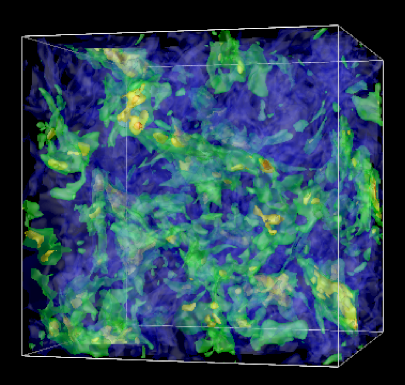
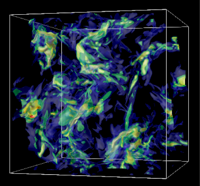
Figure 3: Snapshots of the TVD runs with (a) ${M_{\rm s}}=1$ at $t=5\,\tau_{\rm turb}$, (b) ${M_{\rm s}}=6$ at $t=4.5\,\tau_{\rm turb}$. Note how the turbulent fragmentation of the medium is different for different Mach numbers. Blue, green, yellow, orange, and red colors represent isodensity surfaces with 1, 2, 3, 4 and 5 times the mean density in frame (a). In frame (b), the same order of colors represents isodensity surfaces with 5, 11.25, 17.5, 23.75 and 30 times the mean value.

Figures 3a, b show snapshots of the density field in two TVD simulations with ${M_{\rm s}}=$1 and 6, respectively. The snapshots have been acquired at $t=5\,\tau_{\rm turb}$ (${M_{\rm s}}=1$) and $t=4.5\,\tau_{\rm turb}$ (${M_{\rm s}}=6$). It is evident that the medium is more strongly fragmented in the high Mach number case. A similar conclusion holds for the SPH data cubes. The interactions of supersonic shocks and shocklets in high-RMS Mach flows produce strongly localized density enhancements, and consequently give rise to high degrees of fragmentation even on scales much smaller than the turbulent driving scale.

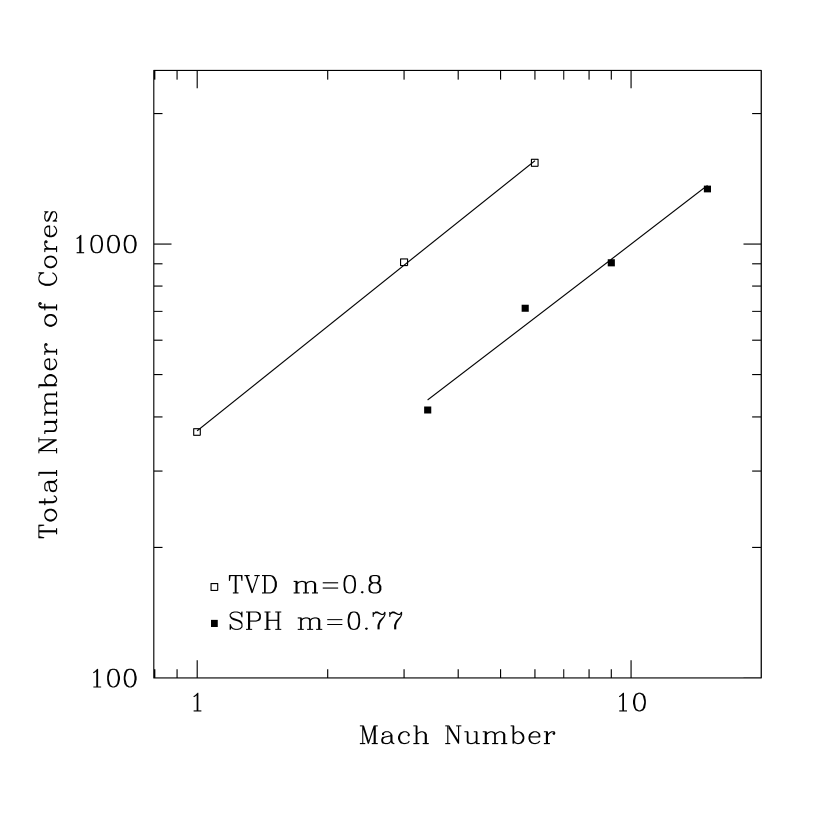
Figure 6: (a) Total number of cores, and (b) Number of cores at maximum of the distribution, as a function of the mach number ${M_{\rm s}}$. Filled (open) squares denote results from SPH (TVD) runs. Solid lines represent least-square fits to the data. $m$ represents the slope of the fit. Note that, for each dataset, the number increases as ${M_{\rm s}}$ increases.

To quantify that further, we present in Figs. 4 and 5 the resulting core mass spectra resulting from the TVD and the SPH models, respectively. The total mass in the computational box for all the models has been renormalized to 64 Jeans masses. The CMD clearly varies with ${M_{\rm s}}$. In particular, the total number of cores as well as the peak value of the histogram increase with ${M_{\rm s}}$. To illustrate this result more clearly we show in Fig. 6 (a) the total number of cores and, (b) the maximum value reached by the histograms as function of ${M_{\rm s}}$. In this figure, filled and open squares correspond to the SPH and the TVD models, respectively. Solid lines in each panel are least-square fits. As a consequence of mass conservation (recall that each TVD and SPH simulation has the same total mass) the typical core mass shrinks as the number of cores increases. This result is shown in Fig. 7, where we plot (a) the mass of the most massive core and, (b) the mass at which the histogram peaks, both as function of ${M_{\rm s}}$.

A point of concern is whether our results depend on the resolution of the simulations. In Fig. 8 we show the CMD resulting from the two high-resolution (HR) simulations. Recall that the HR-TVD runs has $512^{3}$ pixels, while the HR-SPH runs has 9,938,375 particles. This means that the (spatial) resolution is 8 times larger in the TVD-HR case, while the mass resolution in the SPH-HR case is almost 50 times larger. From this figure we stress that the shape of the CMD is, indeed, not a power-law function, but something more similar to a log-normal function, for which the slope varies from zero at the maximum of the distribution to large negative values.

Recall at this point that, since the clumpfinding algorithm in the SPH runs has been used with a smaller density threshold, the typical core mass in the SPH models exceeds that in the TVD case. However, the general trend of increasing number of cores and decreasing core mass with increasing RMS Mach number is independent of the used numerical method as well as the details of the clumpfinding scheme.

4 Discussion

In this section we examine the implications of the results presented in §3, in the context of previous work on the CMD and its relationship with the stellar IMF. We find that the CMD is not a power-law and has a shape that depends on the RMS Mach number. This fact contradicts previous results stating that, in the magnetic case, the CMD follows a power-law whose slope depends on the power index of the kinetic energy spectrum (PN02). As has been mentioned, our simulations do not include magnetic fields and this is an important difference with the work of PN02. However, this fact is not the reason for the differences between the shape of CMD reported in previous section and the power-law they obtain. Indeed, it can be shown that a similar analysis to the one performed by PN02 but for the non magnetic case, also leads to a power-law in which the RMS Mach number of the flow does not enter in the functional form of $N(m)\,d\log{m}$. It only determines the normalization factor, which, in turn, implies that larger $M_{s}$ leads to larger number of cores. Although this fact is consistent with our numerical results (see §3), our results show that the actual shape of the CMD does vary with ${M_{\rm s}}$.

We identify the main reason why the model by PN02 does not include the dependency of the shape of the CMD on ${M_{\rm s}}$ as hinted before: density fluctuations (cores) in a purely turbulent fluid are built-up by a statistical superposition of shocks. This means that mass and density contrast in individual cores grow by a sequence of density jumps with pre-shock densities that can significantly deviate from the mean value $\rho_{0}$ (see, e.g., Smith et al. 2000). In addition, in a turbulent flow with characteristic Mach number ${M_{\rm s}}$, the Mach numbers of the individual shocks may deviate considerably from the mean value ${M_{\rm s}}$. This translates into a large scatter of the Larson (1981) $\delta v-R$ relationship, which has been observed both in theoretical works (e.g., Vázquez-Semadeni et al. 1997; Ostriker et al. 2001; Ballesteros-Paredes & Mac Low 2002), as well as in works that include more recent sets of observations includding different tracers (see Garay & Lizano 1999). Instead, the PN02 model and its hydrodynamic pendant introduced above, assumes that all cores form in one single event with fixed Mach number and initial density. Other caveat in the PN02 model is that stream collisions form sheets, not cores. Thus, the size $\lambda$ of the shock-bounded region may not be a good representative of the size of cores.

If cores are generated not by single shocks, but by statistical superposition of subsequent shocks of the turbulent flow, the dependency of the density structure on the RMS Mach number may have important implications for the fragmentation behavior of molecular clouds, clumps and their cores. For instance, the internal density structure of a dense core (even if it is subsonic) may differ depending whether it is embedded in a highly supersonic, turbulent molecular cloud, or in a more quiescent one (see, e.g., Ballesteros-Paredes et al. 2003, Klessen et al. 2005). For high Mach numbers, the high- frequency part of the turbulent energy cascade lies in the supersonic regime and, hence, is able to produce strong density fluctuations on intermediate to small scales. The amount of energy at the largest scales, where most of the power is, thus, should define the fragmentation on all scales, included those where, the non-thermal motions became subsonic. Thus, we speculate that cores of a given mass in more turbulent clouds (e.g., Orion) will have more substructure than cores of the same mass in less turbulent clouds (e.g., Taurus).

As mentioned in the introduction, there have been various attempts to make a direct connection between the CMD and the stellar IMF. However, the result found in the present work that the CMD has an strong dependence on the Mach number implies that the relationship between these two distributions is not immediate. It is thus important to discus about the possible reasons of this fact in the context of turbulent fragmentation.

The supersonic turbulent motions ubiquitously observed in interstellar clouds, suggest that cores form in first place via shocks, with gravity taking over in the densest and most massive regions. Once gas cores become gravitationally unstable, collapse sets in, but the details of that collapse are not well understood, yet. It is tempting to suggest that turbulence plays a critical role in determining the stellar IMF (see, e.g., the discussion in Ballesteros-Paredes 2005). In this case, the IMF will directly follow from the CMD if individual molecular cloud cores map one-to-one onto stars. However, there is a large number of physical processes that may play an important role during protostellar collapse. Thus, the main problem relating the CMD with the IMF is that a core with a given mass will not necessarily form a star of the same mass, or of a mass that is proportional to the core mass. However, even considering that these effects do not play an important role, and that every core of mass $M$ does indeed produce a star whose mass is directly proportional to $M$, the numerical results presented in this paper suggest that turbulent fragmentation is not the sole agent defining the shape of the IMF, since the shape of the CMD seems not to be a power-law and it varies (as well as the CMD normalization) with the total amount of kinetic energy. Thus, although turbulent fragmentation may play an important role in the determination of the CMD, it is difficult to argue that it is the main ingredient for determining the IMF. In a supersonic turbulent fluid, where the gas is compressed into filaments and sheets, the initial CMD may depend on the parameters of the turbulent gas, however there is still room for other processes to take over and modify the initial CMD in its way to an intermediate mass distribution, and finally to the IMF.

Finally, it has to be mentioned that, although it is generally accepted that the IMF has a slope of $-1.3$ at the high-mass range, the universal character of the IMF is still a debated issue. For instance, Scalo (1998) notes that observations taken at face value reveal variations in the IMF between different star clusters. Kroupa (2001; 2002), on the other hand, argues that these variations can be explained by stellar dynamical processes during the early phases of star-cluster evolution, like mass segregation and the preferred evaporation of low-mass stars. On similar grounds, also Elmegreen (2000) argues in favor of a more universal IMF, although he recognizes statistical deviations.

5 Conclusions

Using two different numerical schemes (TVD and SPH), we have shown that the core mass distribution (CMD) or core mass spectrum from purely turbulent (i.e. without self-gravity and magnetic fields) fragmentation follows a distribution with a continuously varying slope, not necessarily a single power-law. The parameters of this distribution depend on the kinetic energy density in the system as characterized by the RMS Mach number of the flow. Interactions of shocks in high ${M_{\rm s}}$ flows are able to produce strong density fluctuations on small and intermediate scales. We thus speculate that quiescent cores embedded in highly supersonic molecular clouds should exhibit more internal structure than quiescent cores embedded in more quiescent clouds. As consequence, for a molecular cloud of a given mas, the resulting resulting CMD is characterized by a large number of low-mass cores when the Mach number is high. Low-${M_{\rm s}}$ flows, on the other hand, are characterized by small density contrasts and the CMD features fewer cores with on average larger masses.

We conclude that the RMS Mach number of the turbulent flow is a very important parameter that determines the shapes of CMDs. Our calculations indicate that the exact shape of the CMD is not universal, but changes with the Mach number. This calls the existence of a simple one-to-one mapping between the purely turbulent CMD and the observed stellar initial mass function (IMF) into question. Finding the true relation between CMD and IMF instead is a very complex and difficult task, and requires to take additional physical processes into account, such as protostellar feedback from new-born stars (bipolar outflows, winds, and radiation), subfragmentation of individual collapsing protostellar cores into binary and low-$N$ multiple systems, competitive accretion to name just a few.

Figure 1: Temporal evolution of the Mach number (upper panel), number of cores found in the SPH models (middle panel) and in the TVD models (lower panel). Solid lines denote SPH runs, and dotted lines denote TVD runs. Quoted numbers in the upper panel give the mean Mach number, averaged over the frames whose times are larger than 1 turbulent crossing time. (see Table 1). Note that after 1 turbulent crossing time, the fluid has reached equilibrium, since (a) the Mach number becomes nearly constant, with fluctuations not larger than 6.5% (upper panel), and the number of cores has reached its typical value. Note that still fluctuations up to 20% in the number of cores may be found, showing the importance of averaging over several timesteps when calculating CMDs.

Figure 2: Energy spectrum for each simulation. The solid lines correspond to SPH simulations and the dotted lines to TVD simulations. The dashed lines have a slope of $-2$ and $-5/3$.

Figure 4: Time averaged core mass distribution resulting from TVD simulations. The two dot-dashed lines with slopes of $-0.5$ and $-1.3$ are shown for the comparison purpose with the mass functions of Giant Molecular Clouds and protostellar cores, respectively.

Figure 5: Time averaged core mass distribution resulting from SPH simulations. The two dot-dashed lines with slopes of $-0.5$ and $-1.3$ are shown for the comparison purpose with the mass functions of Giant Molecular Clouds and protostellar cores, respectively.

Figure 7: (a) Mass of the most massive core, and (b) mass at which the maximum of the histogram occurs as a function of ${M_{\rm s}}$. Filled (open) squares denote results from SPH (TVD) runs. Solid lines represent least-square fits to the data. $m$ represents the slope of the fit. Note that, for each numeric scheme, the mass decreases as ${M_{\rm s}}$ number increases.

Figure 8: CMD for the high resolution runs using (a) the TVD, and (b) SPH schemes. Note that even at high resolution, a single power-law not necessarily reproduces the high-mass wing of the CMD. Instead, a function that changes more continuously its slope (probably a log-normal function), from zero at maximum, to large negative values for increasing masses, may reproduce better the distribution.

References

- Ballesteros-Paredes (2005) Ballesteros-Paredes, J. 2005, Ap&SS, in press
- Ballesteros-Paredes et al. (2003) Ballesteros-Paredes, J., Klessen, R. S., & Vázquez-Semadeni, E. 2003, ApJ, 592, 188
- Ballesteros-Paredes & Mac Low (2002) Ballesteros-Paredes, J. & Mac Low, M. 2002, ApJ, 570, 734
- Ballesteros-Paredes, Vázquez-Semadeni, & Scalo (1999) Ballesteros-Paredes, J., Vázquez-Semadeni, E., & Scalo, J. 1999, ApJ, 515, 286
- Bate & Bonnell (2004) Bate, M. R., & Bonnell, I. A. 2004, MNRAS, 728
- Benz (1990) Benz, W. 1990, in The Numerical Modeling of Nonlinear Stellar Pulsations, ed. J. R. Buchler (Dordrecht: Kluwer), 269
- Chabrier (2003) Chabrier, G. 2003, PASP, 115, 763
- Elmegreen (1993) Elmegreen, B. G. 1993, ApJ, 419, L29
- Elmegreen (2000) Elmegreen, B. G. 2000, ApJ, 539, 342
- Gammie, Lin, Stone, & Ostriker (2003) Gammie, C. F., Lin, Y., Stone, J. M., & Ostriker, E. C. 2003, ApJ, 592, 203
- Garay & Lizano (1999) Garay, G., & Lizano, S. 1999, PASP, 111, 1049
- Goodwin et al. (2004) Goodwin, S. P., Whitworth, A. P., & Ward-Thompson, D. 2004, A&A, 423, 169
- Hartmann (2001) Hartmann, L. 2001, AJ, 121, 1030
- Hunter & Fleck (1982) Hunter, J. H., & Fleck, R. C. 1982, ApJ, 256, 505
- Jappsen et al. (2005) Jappsen A. K., Klessen R. S., Larson, R. B., Li Y., & Mac Low, M. M., 2005, A&A, 435, 611
- Kim et al. (1999) Kim, J., Ryu, D., Jones, T. W., & Hong, S. S. 1999, ApJ, 514, 506
- Kim et al. (2005) Kim, J.S. et al. 2005. ApJ, submitted
- Klessen (2001) Klessen, R. S. 2001, ApJ, 556, 837
- Klessen et al. (2005) Klessen, R. S., Ballesteros-Paredes, J., Vázquez-Semadeni, E., & Durán-Rojas, C. 2004, ApJ, 620,786
- Klessen & Burkert (2000) Klessen, R. S., & Burkert, A. 2000, ApJS, 128, 287
- Klessen et al. (2000) Klessen, R. S., Heitsch, F., & Mac Low, M. 2000, ApJ, 535, 887
- Klessen & Lin (2003) Klessen, R. S., & Lin, D.N.C. PRE, 67, 036311
- Kroupa (2001) Kroupa, P. 2001, MNRAS, 322, 231
- Kroupa (2002) Kroupa, P. 2002, Astronomical Society of the Pacific Conference Series, 285, 86
- Larson (1981) Larson, R. B. 1981, MNRAS, 194, 809
- Larson (1985) Larson, R. B. 1985, MNRAS, 214, 379
- Larson (2005) Larson, R. B. 2005, MNRAS, 359, 211
- Li, Klessen & Mac Low (2003) Li, Y., Klessen, R. S., & Mac Low, M. M. 2003, ApJ, 592, 233L
- Li et al. (2004) Li, P. S., Norman, M. L., Mac Low, M., & Heitsch, F. 2004, ApJ, 605, 800
- Mac Low & Klessen (2004) Mac Low, M., Klessen, R. S. 2004, RvMP, 76, 125
- Meyer et al. (2000) Meyer, M. R., Adams, F.C., Hillenbrand, L.A., Carpenter, J.M., & Larson, R.B. 2000, in Protostars and Planets IV, ed. V. Mannings, A. P. Boss, & S. S. Russell (Tuscon: Univ. Arizona Press), 121
- Motte et al. (1998) Motte, F., André, P., & Neri, R. 1998, A&A, 336, 150
- Ossenkopf et al. (2001) Ossenkopf, V., Klessen, R. S., & Heitsch, F. 2001, A&A, 379, 1005
- Ostriker, Stone, & Gammie (2001) Ostriker, E. C., Stone, J. M., & Gammie, C. F. 2001, ApJ, 546, 980
- Padoan, Juvela, Goodman, & Nordlund (2001) Padoan, P., Juvela, M., Goodman, A. A., & Nordlund, Å. 2001b, ApJ, 553, 227
- Padoan & Nordlund (2002) Padoan, P., & Nordlund, Å. 2002, ApJ, 576, 870
- Passot & Vazquez-Semadeni (1998) Passot, T., & Vázquez-Semadeni, E. 1998, PhRvE, 58, 4501
- Salpeter (1955) Salpeter, E. E. 1955, ApJ, 121, 161
- Sasao (1973) Sasao, T. 1973, PASJ, 25, 1
- Scalo (1998) Scalo, J. 1998, in The Stellar Initial Mass Function (38th Herstmonceux Conference), G. Gilmore & D. Howell eds. ASPC, 142, 201
- Scalo & Elmegreen (2004) Scalo, J., & Elmegreen, B. G. 2004, ARA&A, 24,275
- Scalo et al. (1998) Scalo, J., Vázquez-Semadeni, E., Chappell, D., & Passot T. 1998, ApJ, 504, 835
- Schmeja & Klessen (2004) Schmeja, S., & Klessen, R. S. 2004, A&A, 419, 405
- Smith et al. (2000) Smith, M. D., Mac Low, M.-M., & Heitsch, F. 2000, A&A, 362, 333
- Spitzer (1978) Spitzer, L. 1978. Physical processes in the interstellar medium, New York Wiley-Interscience
- Springel et al. (2001) Springel, V., Yoshida, N., & White, S. D. M. 2001, New Astronomy, 6, 79
- Stone, Ostriker, & Gammie (1998) Stone, J. M., Ostriker, E. C., & Gammie, C. F. 1998, ApJ, 508, L99
- Tilley & Pudritz (2004) Tilley, D. A., & Pudritz, R. E. 2004, MNRAS, 353, 769
- Testi & Sargent (1998) Testi, L., & Sargent, A. I. 1998, ApJ, 508, 91
- Vazquez-Semadeni (1994) Vázquez-Semadeni, E. 1994, ApJ, 423, 681
- Vazquez-Semadeni et al. (1997) Vázquez-Semadeni, E., Ballesteros-Paredes, J., & Rodriguez, L. F. 1997, ApJ, 474, 292
- Vazquez-Semadeni et al. (2000) Vázquez-Semadeni, E., Ostriker, E. C., Passot, T., Gammie, C. F., & Stone, J. M. 2000, Protostars and Planets IV, 3
- Williams et al. (1994) Williams, J. P., de Geus, E. J., & Blitz, L. 1994, ApJ, 428, 693