Testing Bekenstein’s Relativistic MOND with Lensing Data

Abstract

We propose to use multiple-imaged gravitational lenses to set limits on gravity theories without dark matter, specificly TeVeS (Bekenstein 2004), a theory which is consistent with fundamental relativistic principles and the phenomenology of MOdified Newtonian Dynamics (MOND) theory. After setting the framework for lensing and cosmology, we derive analytically the deflection angle for the point lens and the Hernquist galaxy profile, and study their patterns in convergence, shear and amplification. Applying our analytical lensing models we fit galaxy-quasar lenses in the CASTLES sample. We do this with three methods, fitting the observed Einstein ring sizes, the image positions, or the flux ratios. In all cases we consistently find that stars in galaxies in MOND/TeVeS provide adequate lensing. Bekenstein’s toy $\mu$ function provides more efficient lensing than the standard MOND $\mu$ function. But for a handful of lenses a good fit would require a lens mass orders of magnitude larger/smaller than the stellar mass derived from luminosity unless the modification function $\mu$ and modification scale $a_{0}$ for the universal gravity were allowed to be very different from what spiral galaxy rotation curves normally imply. We discuss the limitation of present data and summarize constraints on the MOND $\mu$ function. We also show that the simplest TeVeS ”minimal-matter” cosmology, a baryonic universe with a cosmological constant, can fit the distance-redshift relation from the supernova data, but underpredicts the sound horizon size at the last scattering. We conclude that lensing is a promising approach to differentiate laws of gravity (see also astro-ph/0512425).

1 Introduction

The standard paradigm of Einsteinian gravity with dark matter and dark energy has proven amazingly successful at describing the Universe, in particular the data from the Cosmic Microwave Background (e.g. Spergel et al 2003), galaxy redshift surveys (Percival et al 2002, Tegmark et al 2004), Type Ia supernovae (Reiss et al 1998, Perlmutter et al 1999), and weak gravitational lensing (see e.g. van Waerbeke & Mellier 2003, Refregier 2003 for reviews) to high accuracy with a small number of parameters. However, it is worth exploring alternative models of gravity to assess the uniqueness of the model and to open up new ways to unify gravity and the standard model. Indeed, the detection of deviations from the Einstein-Hilbert action could signal new physics, and such deviations are expected, for example, in models such as the M-theory inspired braneworld.

The central role of both dark matter and dark energy in the cosmological model has also led some workers to question the standard paradigm. Given this it seems sensible to develop methods to test the basic assumptions of this paradigm, if only to put them on a firmer basis. One of the most direct ways to probe gravity over large scales in the Universe is via the effect of gravitational lensing.

In this paper we shall explore gravitational lensing in the recently developed relativistic version of Modified Newtonian Dynamics (MOND), the Tensor-Vector-Scalar (TeVeS) theory, developed by Bekenstein (2004). The non-relativistic version of MOND was originally proposed by Milgrom (1983) as an alternative to the dark matter paradigm. Milgrom (1983) suggested that galaxy rotation curves $V(r)$ could be explained by modifying gravity:

$$g=\frac{V^{2}}{r}=\frac{GM}{r^{2}\mu},~{}\mu=\cases{{g\over a_{0}}&$g\ll a_{0}\approx 1.2\times 10^{-8}{\rm cm}s^{-2}$.\cr 1&$g\gg a_{0}$,\cr}$$ (1)

where the interpolation function $\mu(g/a_{0})$ is the effective “dielectric constant”, which itself has the above asymptotic dependence on the gravitational field strength, $g$. Thus the gravitational field strength $g$ becomes significantly stronger than Newtonian gravity $GM/r^{2}$ in the weak MOND regime, when $g\leq a_{0}$.

From a theoretical point of view, MOND has not just one extra free parameter, $a_{0}$, which is tuned to explain Tully-Fisher relations, but also a free interpolation function, $\mu(g/a_{0})$. With a standard choice $\mu(x)={x\over\sqrt{1+x^{2}}}$, one can achieve very good fits to contemporary kinematic data of a wide variety of high and low surface brightness spiral and elliptical galaxies; even the fine details of velocity curves are reproduced without fine tuning of the baryonic model (Sanders & McGaugh, 2002; Milgrom & Sanders, 2003). However, whether MOND qualifies as a gravitational theory depends on its prediction of fundamental properties of gravity, e.g., the bending of the light.

In a more rigorous treatment of MOND (Bekenstein & Milgrom, 1984), gravity is the gradient of a conserved potential, $\Phi(\mbox{\boldmath$r$})$. It satisfies a modified Poisson’s equation, and trajectories of massive particles are governed by the equation of motion as follows,

$${d^{2}\mbox{\boldmath$r$}\over dt^{2}}=\mbox{\boldmath$g$}=-\mbox{\boldmath$\nabla$}\Phi(\mbox{\boldmath$r$}),\qquad\mbox{\boldmath$\nabla$}.\left[\mbox{\boldmath$g$}\mu(g/a_{0})\right]=-4\pi G\rho,$$ (2)

where the right-hand equation is the density of all baryonic particles, $g=|\mbox{\boldmath$g$}|$ is the magnitude of the gravitational field.

These versions of MOND, however, all suffer from being non-relativistic. The main problem is that the theory is not generally covariant, as the physics still depends on the measured local acceleration. In the absence of a relativistic version of MOND, the paradigm could not be used to build cosmological models and could not provide robust predictions for the expanding Universe, the Cosmic Microwave Background, the evolution of perturbations, and gravitational lensing.

Recently a fully relativistic, generally covariant version of MOND has been proposed, TeVeS (Bekenstein 2004), which passes standard local and cosmological tests used to check General Relativity. In this relativistic version, the conformal freedom of a general relativistic model is used, along with a new scalar field, one vector field and a conformally coupled metric tensor, to preserve general covariance. Following Bekenstein’s (2004) paper, a number of other works have appeared studying the cosmological model (Hao & Akhoury, 2005) and large-scale structure of the Universe (Skordis et al., 2005) in the relativistic TeVeS theory. There are also attempts to refine the Lagrangian for the scalar field in TeVeS (hence the MOND interpolation $\mu$-function) to improve fits to galaxy rotation curves (Famaey & Binney 2005) and avoid unphysical dilation effects in two-body systems (Zhao & Famaey 2005). A further extention of TeVeS, dubbed BSTV, has also been recently developed by Sanders (2005), which adds more flexibilities into the theory by making one of the non-dynamical scalar field in TeVeS a dynamical field. It remains to be seen what the range of predictions of these theories are in cosmology and solar system dynamics.

Our goal here is to develop and test TeVeS by making concrete predictions of lensing in the theory, and comparing these predictions to data from strong lensing. We present the general framework for lensing in TeVeS. As a first application to data, we apply models of simple axisymmetric lenses: the point-mass lens and the Hernquist profile. While the point-mass is a very poor model for galaxies in a dark matter theory, it is a reasonable model for lensing in TeVeS, where the baryons are concentrated in a central region, and the Einstein ring in most strong lenses encloses most of the baryons of the galaxy. As an extension to this, we also consider the Hernquist profile, which allows us to develop our analysis to include extended galaxies.

Our lensing formulation bears similarities with that of Qin et al. (1995), who developed a heuristic formulation to compute lensing in MOND in the weak field regime. Here we develop a more rigorous approach based on the relativistic TeVeS. In the weak-field regime of Bekenstein’s model we find a bending angle a factor of two greater than that found by Qin et al. (1995), consistent with GR.

As reviewed by Bekenstein (2004) and Sanders (2005), there are probably many ways of generalising MOND to a relativistic theory, with TeVeS (or BSTV) being the most successful one so far. Although we derive our results within the framework of the TeVeS theory, we explore a regime where dynamics behaves like in MOND. Therefore our results are likely relavent for other relativistic versions of MOND as well.

Nevertheless fundamental differences exist between MOND and TeVeS, not only at the conceptual level, but also at the phenomenology level, particularly when dealing with a non-spherical potential with tide or external field. For example, the Roche lobe of a satellite in MOND is more squashed in MOND than naive extrapolations of the Newtonian result (Zhao 2005), and the shape depends on the MOND function $\mu$ (Zhao & Tian 2005) or the TeVeS $\mu$ for the scalar field (Zhao & Famaey 2005). Major development is also made in numerical tools to solve MONDian Poisson’s equations for studying systems of a general geometry in detail (Ciotti et al. 2005). For these reasons, we prefer to follow the TeVeS formulation of lensing and cosmology instead of previous phenomenology-based formulations (Qin et al. 1995, Mortlock & Turner 2001).

The paper is set out as follows. After a brief presentation of the basic equations of Bekenstein’s TeVeS theory in §2. We give in §3 the central equations for gravitational lensing, and show how to calculate gravitational potential around a galaxy. An eager reader could go directly to §4, where we model distances and ages in a homogeneous and isotropic, expanding universe, and determine the parameters for the minimal-matter cosmology by fitting the high-z SNe distances. In §5 we derive the effects of lensing by a point-mass lens. This model is then generalised to a Hernquist profile in §6 and applied to observed galaxy-quasar lenses in §7. We present our conclusions in §8.

2 The TeVeS Equations And Approximations For Galaxies

Bekenstein’s theory involves two metrics, one of which we denote by $g_{\mu\nu}$ and is the metric in the Einstein frame, and the other is the physical metric which couples to matter, $\tilde{g}_{\mu\nu}$, following the notation of Bekenstein. The two metrics (and their inverses) are related by

$$\tilde{g}_{\mu\nu}=e^{-2\phi}g_{\mu\nu}+(e^{-2\phi}-e^{2\phi})U_{\mu}U_{\nu},$$ (3)

where $\phi$ is a dynamical scalar field and $U^{\mu}\equiv g^{\mu\nu}U_{\nu}$ is a dynamical, time-like vector field, normalised by $g^{\mu\nu}U_{\nu}U_{\mu}=1$. Note that $\tilde{g}_{\mu\nu}=g_{\mu\nu}$ in the limit that the scalar field $\phi=0$. The dynamics of the vector field are governed by an action (cf. eq. 26 of Bekenstein), but for the problems involving lensing, which deal with either a static galaxy or a homogeneous universe, the vector field simplifies in the Einstein frame to

$$U^{\mu}=[(-g_{tt})^{-{1\over 2}}c,0,0,0],$$ (4)

i.e., a four-vector which is parallel to the time axis apart but with a different normalisation. The gravity sector of the theory is given by the Einstein-Hilbert action in the Einstein frame,

$$S_{g}=\int\!d^{4}x\,\sqrt{-g}g^{\mu\nu}\left({R_{\mu\nu}\over 16\pi G_{K}}+{\rho_{\Lambda}c^{2}g_{\mu\nu}\over 2}\right),$$ (5)

where $G_{K}$ is a parameter of the theory, and here $g$ is the determinant of the metric tensor, $R_{\mu\nu}$ is the Ricci tensor in the Einstein frame, and $\rho_{\Lambda}c^{2}$ is the energy density due to a cosmological constant. Matter is coupled to the physical metric by the usual action $S_{m}=\int\!d^{4}x\,\sqrt{-\tilde{g}}{\cal L}_{m}$ where ${\cal L}_{m}$ is the Lagrangian for the luminous matter fields. Hence the physical energy momentum tensor

$$\tilde{T}_{\mu\nu}=\left[(\tilde{\rho}c^{2}+\tilde{p})\tilde{u}_{\mu}\tilde{u}_{\nu}+\tilde{p}\tilde{g}_{\mu\nu}\right],\qquad\tilde{u}_{\mu}={\rm e}^{\phi}U_{\mu},$$ (6)

where the renormalised physical four-velocity, $\tilde{u}_{\mu}$, is treated as colinear with the time-like field, $U_{\mu}$. The scalar field, $\phi$ is governed by an additional action (cf. equation 25 of Bekenstein 2004). As a result, the scalar field $\phi$ tracks the matter energy-momentum tensor distribution, satisfying an equation,

$$\left[{\tilde{\mu}\over 1-\tilde{\mu}}\phi^{,\nu}\right]_{;\nu}=4\pi G_{K}c^{-4}\left[g^{\mu\nu}+(1+{\rm e}^{-4\phi})U^{\mu}U^{\nu}\right]\tilde{T}_{\mu\nu},$$ (7)

where $\tilde{\mu}(\delta_{\phi}^{2})$ is a function of $\delta_{\phi}^{2}$ , which is defined by

$$\delta_{\phi}^{2}\equiv{\phi^{,\nu}\phi_{,\nu}c^{4}\over a_{0}^{2}},\qquad\phi^{,\nu}\equiv(g^{\mu\nu}-U^{\mu}U^{\nu})\phi_{,\mu}.$$ (8)

Here $\tilde{\mu}$ and $\delta_{\phi}^{2}$ are non-dynamical fields, i.e., they are some fixed functions of the scalar field $\phi$ and the metric $g_{\mu\nu}$. As will become obvious $a_{0}$ can be identified with the acceleration scale in MOND.

Near a galaxy the scalar field, $\phi$, is quasi-static, hence we can neglect all time derivatives compared to spatial derivatives so that

$$\delta_{\phi}^{2}\approx{|\mbox{\boldmath$\nabla$}\phi|^{2}c^{4}\over a_{0}^{2}},\qquad\phi_{,\mu}\approx\phi^{,\mu}=(0,\mbox{\boldmath$\nabla$}\phi).$$ (9)

Bekenstein argues that in the Einstein frame $g_{tt}\approx{\rm e}^{-2\phi}\tilde{g}_{tt}\approx-{\rm e}^{2\Phi_{N}/c^{2}}c^{2}$, with $\Phi_{N}(\mbox{\boldmath$r$})\equiv\Phi(\mbox{\boldmath$r$})-\phi(\mbox{\boldmath$r$})c^{2}$. Substituting these, and a simplified energy momentum tensor (equation 6), into equation (7) for the scalar. Drop the pressure term, time derivatives and higher order terms, which are all small compared to the physical matter density term, $\tilde{\rho}$, the equation now starts to resemble Poisson’s equation,

$$2\mbox{\boldmath$\nabla$}\cdot\mbox{\boldmath$\nabla$}\Phi_{N}\approx 2\mbox{\boldmath$\nabla$}\cdot\left[{\tilde{\mu}\over 1-\tilde{\mu}}\mbox{\boldmath$\nabla$}\phi c^{2}\right]\approx 8\pi\widetilde{G}\tilde{\rho},~{}\widetilde{G}\equiv G_{K}{\rm e}^{-2\phi_{c}},$$ (10)

where we set $\phi\approx\phi_{c}$, which is the cosmological average of $\phi$, and define $\widetilde{G}$ as the physical gravitational constant. Hence $\Phi_{N}(\mbox{\boldmath$r$})$ is basically the Newtonian gravitational potential, and is related to the physical matter density by the Newtonian Poisson’s equation. The equation of motion in these potentials is

$${d^{2}\mbox{\boldmath$r$}\over d\tilde{t}^{2}}=-\mbox{\boldmath$\nabla$}\Phi(\mbox{\boldmath$r$})=-\mbox{\boldmath$\nabla$}\Phi_{N}(\mbox{\boldmath$r$})-\mbox{\boldmath$\nabla$}\phi(\mbox{\boldmath$r$})c^{2},$$ (11)

The above two equations link the gravitational potential $\Phi$, the scalar field $\phi$, the matter density $\tilde{\rho}$ and the motion $d\mbox{\boldmath$r$}/dt$ together. Plus a certain choice of the free interpolation function, we fully specify the dynamics near a galaxy. As a first study we adopt a very simple choice of the free function with

$$\delta_{\phi}^{2}=\cases{\tilde{\mu}^{2}(1-\tilde{\mu})^{2},&\quad$0\leq\tilde{\mu}\leq 1$,\cr 0&\quad otherwise .\cr}$$ (12)

As will become obvious, this choice of $\delta_{\phi}^{2}$ is necessary to simplify the analytics of lensing by an extended galaxy.

To suit our studies, here we have chosen a set of notations slightly different from Bekenstein. We avoid using Bekenstein’s $\mu$ completely, which does not have the same role as Milgrom’s $\mu$, which is a function of gravity $g=|\mbox{\boldmath$\nabla$}\Phi|$. To distinguish from Milgrom’s $\mu(g/a_{0})$ as well, we use $\tilde{\mu}(\delta_{\phi}^{2})$ to emphasise its dependence on the scalar field strength, not the overall gravity.

In our notations the toy model proposed by Bekenstein (his eq. 50) related $\delta_{\phi}^{2}$ and $\tilde{\mu}$ by

$$\delta_{\phi}^{2}={\tilde{\mu}^{2}\over(1-\tilde{\mu})^{2}}\left[{(1-{(1-K/2)k\over 8\pi}{\tilde{\mu}\over 1-\tilde{\mu}})^{2}\over(1-{(1-K/2)k\over 4\pi}{\tilde{\mu}\over 1-\tilde{\mu}})}\right],$$ (13)

where the parameters $k$ and $K$ are much less than unity. Fig. 1 compares these Bekenstein’s toy model with our toy model. Our choice is different from Bekenstein’s choice which allows a $\delta_{\phi}^{2}$ with no upper limit and with a negative branch with subtle effects on cosmology. Nevertheless, both choices preserve the asymptotic relation $\tilde{\mu}\rightarrow\delta_{\phi}$ in the weak gravity limit, which is essential for explaining galaxy rotation curves, the main success of MOND. We have also made lensing predictions for scalar field closely matching Bekenstein’s toy model, this is given in the Discussion section.

Figure 1: shows the scalar field strength $\delta_{\phi}^{2}$ as function of $\tilde{\mu}$ in Bekenstein’s toy models (region shaded by dots with $k$ and $K$ between $0$ and $10$). Also shown is our principal model (solid line cf. eq. 12), and the smooth model (dashed line at the lower boundary Bekenstein models, cf. eq. 80)

3 Lensing and Potential in TeVeS

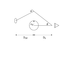
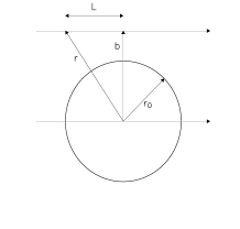
Figure 2: Schematics of the lens geometry considered in this section. Top: Overall geometry. We indicate the angular diameter distance from observer to lens, $D_{l}$ and lens to source, $D_{ls}$, the observed image angle $\theta$, the bend angle $\alpha$ and radius of Newtonian bubble $r_{0}$. Bottom: The geometry of a light beam past a point lens, indicating the position of a photon distance from the point-source, $r$, the distance of closest approach, $b$ and the radius of the ”Newtonian bubble”, $r_{0}=\sqrt{GM/a_{0}}$.

3.1 Bending of Light Rays in Slightly Curved Space Time

Light rays trace the null geodesics of the space time metric. Lensing, or the trajectories of light rays in general, are uniquely specified once the metric is given. In this sense light bending works exactly the same way in any relativistic theory as in GR.

Near a quasi-static system like a galaxy, the physical space-time is only slightly curved, and can be written in polar coordinates as

$$-c^{2}d\tau^{2} \approx {\rm e}^{2\Phi/c^{2}}c^{2}d\tilde{t}^{2}+{\rm e}^{-2\Phi/c^{2}}dl^{2},$$ (14)

$$dl^{2} = (dr^{2}+r^{2}d\theta^{2}+r^{2}\sin^{2}\theta d\psi^{2}).$$ (15)

where $|\Phi(\mbox{\boldmath$x$})|\leq c^{2}$ takes the meaning of a gravitational potential in a rectangular coordinate $\mbox{\boldmath$x$}=(x_{1},x_{2},x_{3})$ centred on the galaxy, we note that a non-relativistic massive particle moving in this metric follows the geodesic ${d^{2}\mbox{\boldmath$x$}\over d\tilde{t}^{2}}\approx-\mbox{\boldmath$\nabla$}\Phi(\mbox{\boldmath$x$})$, which is the equation of motion in the non-relativistic limit.

Consider lensing by the potential $\Phi(\mbox{\boldmath$r$})$ of a galaxy with a geometry as in Fig. 2. An observed light ray travels a proper distance $l_{os}=l_{ls}+l_{ol}$ from a source to the lens and then to an observer. Hence it arrives after a time interval (seen in polar coordinates by an observer at rest with respect to the lens)

$$\tilde{t}\approx\int_{0}^{l_{os}}{\rm e}^{-2\Phi({\bf r})/c^{2}}{dl\over c}\approx\int_{0}^{l_{os}}{dl\over c}-\int_{0}^{l_{os}}{2\Phi({\bf r})\over c^{2}}{dl\over c},$$ (16)

where we used the fact that a light ray moving with a constant speed $c$ inside follows the null geodesics $d\tau=0$. As in an Einstein universe (c.f. Bartelmann & Schneider 2001), the arrival time contains a geometric term and a Shapiro time delay term due to the $\Phi$ potential of a galaxy. Gravitational time delay hence works as in GR, but with $\Phi$ instead of the Newtonian gravitational potential, $\Phi_{N}(\mbox{\boldmath$r$})$. Note that we recover the GR-like factor of two in front of $\Phi$. Images will be on extrema points of the light arrival surface, hence the factor of two propagates to the deflection angle as well. Hence, to a good approximation, lensing by galaxies in TeVeS behaves as in GR apart from different interpretations of the gravitational potential.

For example, assume a spherical lens with a potential $\Phi(r)$. A light ray with an impact parameter $b$, we can reduce the eq. (109) of Bekenstein to

$$\alpha(b)\approx\int_{b}^{\infty}{dr\over c^{2}}{4b\over\sqrt{r^{2}-b^{2}}}{d\Phi(r)\over dr},$$ (17)

where we take the weak field and thin lens approximation (i.e., we can drop higher order terms, assume the lens is far from the observer, the source $l_{ls}\rightarrow\infty$ and $l_{ol}\rightarrow\infty$, and approximating the closest approach $r_{\rm min}\approx b$). Interestingly this is twice the bending angle predicted from extrapolating non-relativistic dynamics (Qin et al. 1995).

In fact, gravitational lensing in TeVeS recovers many familiar results of Einstein gravity even in non-spherical geometries. For example, an observer at redshift $z=0$ sees a delay $\Delta t_{\rm obs}$ in the light arrival time due to a thin deflector at $z=z_{l}$

$${\Delta t_{\rm obs}({\bf R})\over(1+z_{l})}\approx{D_{s}\over 2D_{l}D_{ls}}\left({\bf R}-{\bf R}_{s}\right)^{2}-\int_{-\infty}^{\infty}\!\!\!dl{2\Phi({\bf R},l)\over c^{2}},$$ (18)

as in GR for a weak-field thin lens, $\Phi/c^{2}\ll 1$. A light ray penetrates the lens with a nearly straight line segment (within the thickness of the lens) with the 2-D coordinate, $\mbox{\boldmath$R$}=D_{l}\mbox{\boldmath$\theta$}$, perpendicular to the sky, where $D_{l}(z_{l})=l_{ol}/(1+z_{l})$ is the angular (diameter) distance of the lens at redshift $z_{l}$, $D_{s}$ is the angular distances to the source, and $D_{ls}$ is the angular distance from the lens to the source. The usual lens equation can be obtained from the gradient of the arrival time surface with respect to $R$.

Nevertheless, there are important differences between lensing in TeVeS and in GR. These are mainly in the predicted metric for a given galaxy mass distribution, and the predicted metric and distance-redshift relation for the Hubble expansion, which we will come to.

There are, however, conceptual differences between TeVeS and MOND. The modification of gravity in TeVeS is made through the factor $\tilde{\mu}(|\mbox{\boldmath$\nabla$}\phi|^{2}c^{4}a_{0}^{-2})$, hence depends on the scalar field gradient $|\mbox{\boldmath$\nabla$}\phi|$, rather than $|\mbox{\boldmath$\nabla$}\Phi|$ as in MOND. Strictly speaking, $\mbox{\boldmath$\nabla$}\phi$ and $\mbox{\boldmath$\nabla$}\Phi$ are generally not colinear except for special geometries, hence the two descriptions are not generally identical.

In short Bekenstein’s theory reduces to MOND in the non-relativistic and spherical limit. Later in the paper, we will work exclusively under the assumption that $\phi\sim\phi_{c}\sim 0$, or ${\rm e}^{\phi}\sim 1$. Hence we can drop the tilde sign without confusion. We will consider spherical systems only, where the magnitude of the gravitation field is given by equation (11), and $a_{0}$ is given by equation (1).

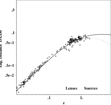
Figure 3: Upper panel: Angular diameter distance $D_{A}(z)$ (in units of the MOND critical distance $D_{0}=c^{2}a_{0}^{-1}\sim 6cH_{0}^{-1}$) vs. redshift , $z$, in two cosmologies: $(\Omega_{m},\Omega_{\Lambda})=(0.04,0.46)$ (”minimal-matter” cosmology, thick solid) and $(0.25,0.75)$ (LCDM, thin dashed). The data are converted to angular diameter distances by multiplying by a factor $(1+z)^{-2}$ and assuming $H_{0}=70\,{\rm km}s^{-1}{\rm Mpc}^{-1}$. We also label typical lenses at redshifts $z=0.1$ – $1$, and typical quasar sources at redshifts $z=1$ – $3$ (as labelled). Note ${D_{A}(z)\over D_{0}}\ll 1$ at all redshifts due to the low value of $a_{0}$, which means that cosmological objects have too small angular diameter distances for any prominent deep-MOND effect in lensing, i.e., most of the bending is done in the Newtonian bubble of Fig. 2). Middle panel: The minimal-matter cosmology (TeVeS) fit to high-z SN Ia luminosity distance modulus is slightly poorer than the $\Lambda$CDM flat cosmology fit, although only by $\Delta\chi^{2}=3.5$ or $1.9\sigma$; error bars indicate the $\pm 1\sigma$ limit on the estimated $\Omega_{\Lambda}$. Bottom panel: shows for models of different $\Omega_{\Lambda}$ the sound horizon at $z=1000$ (in degrees) in the above ”minimal-matter” open cosmology and CDM-based closed cosmology.

4 Angular Diameter Distances for Lensing in a simplistic minimal-matter open cosmology

To describe gravitational lensing, it is essential to know how the background cosmology behaves in Bekenstein’s TeVeS. Lensing requires knowing the luminosity distance $D_{L}(z)$ and the angular diameter distance $D_{A}$ in a universe as functions of redshift. These can be predicted generally by

$${D_{L}(z)\over(1+z)^{2}}=D_{A}(z)={c\over(1+z)}{\sinh\left[\Omega_{K}^{1/2}\int_{0}^{z}{dz\over H(z)}\right]\over\Omega_{K}^{1/2}}.$$ (19)

where $\Omega_{K}$ is the usual curvature density parameter and $H(z)$ is the Hubble expansion rate. To develop the cosmological model, we assume an isotropic and homogeneous physical metric in TeVeS (cf. equations 117 and 118 of Bekenstein);

$$-c^{2}d\tau^{2}=-c^{2}d\tilde{t}^{2}+\tilde{a}(\tilde{t})^{2}\left[d\chi^{2}+\sinh\chi^{2}\left(d\theta^{2}+\sin\theta^{2}d\psi^{2}\right)\right]$$ (20)

for an open universe with the expansion factor $\tilde{a}$ and the cosmological time $\tilde{t}$.

We are interested in lensing in a reasonable cosmological model in TeVeS context, which should be in accord with Supernovae (SNIa) data. There are many degrees of freedom in TeVeS, which is beyond the exploration of this paper. One way is to consider a ”mininal cosmology” in TeVeS context with just a low density baryonic universe plus some amount of cosmological constant model such that to fit SNe data. As argued by Bekenstein, the scalar field contributes negligibly to the Hubble expansion, with a ratio $O(k)$ compared to the matter contribution, and $k$ is small. Hence the minimal-matter cosmological model is largely the same as in the case of GR, and for latter discussion we set the energy density of the scalar field $\rho_{\phi}=0$ (c.f. Section VII, Bekenstein 2004). Under this crude approximation, we find that the Hubble parameter $H(z)$ is given by

$${\dot{\tilde{a}}^{2}\over\tilde{a}^{2}}=H^{2}(z)\approx H_{0}^{2}\left(\Omega_{m}(1+z)^{3}+\Omega_{\Lambda}+\Omega_{K}(1+z)^{2}\right),$$ (21)

where $\Omega_{K}\approx 1-\Omega_{\Lambda}-\Omega_{m}$. At low redshift the vacuum energy is important and dominating. Choosing an appropriate vacuum energy, it is conceivable that one can make a TeVeS baryonic universe which expands at virtually the same rate as the CDM model. For example, we find a reasonable fit is an open cosmology with $\Omega_{\Lambda}\sim 0.46$, $\Omega_{m}\sim 0.03$, and $H_{0}\sim 70$km/s/Mpc. It is possible to fit the luminosity distances of high-z SNe about as well as CDM up to a redshift of 1 – 2. Fig. 3 show the angular diameter distance as a function of redshift, for a best-fit minimal-matter cosmology and a standard $\Lambda$CDM model. Clearly both models are consistent with the high-z SNe distance moduli data set; the minimal-matter cosmology fit is slightly poorer than the $\Lambda$CDM fit, but only by 1.9$\sigma$ and is therefore admissible. This open cosmology has problems at very high redshift, e.g., the last scattering sound horizon will be too small. This undesirable feature might be an artifact of the our simple cosmology, rather than intrinsic to TeVeS; e.g., allowing for $2$eV neutrino Dark Matter to co-exist with baryonic matter in MOND would soften the problems (Sanders 2003). More detailed analysis is clearly needed. Despite its limitations our simplistic minimal-matter cosmology is sufficient for assigning lensing and source distances in redshift $z=1-3$.

Table 1: Lookup-table for our notations for lensing in TeVeS

Parameters	Meaning
$a_{0}$	Threshold for weak acceleration regime
$g$	Gravity strength $|{\bf\nabla}\Phi|$ in TeVeS
$g_{N}$	Newtonian gravity strength $|{\bf\nabla}\Phi_{N}|$
$\mu(g)$ or $\tilde{\mu}(\delta_{\phi}^{2})$	Interpolation function
${\bf\nabla}\phi c^{2}=a_{0}\sqrt{|\delta_{\phi}|}$	Scalar field strength in quasi-static galaxies
$D_{l}$	Angular diameter distance to lens
$D_{s}$	Angular diameter distance to source
$D_{ls}$	Angular distance from lens to source
$D_{0}=c^{2}/a_{0}$	Distance scale of weak acceleration
$\xi={\eta^{2}\over 4}={D_{l}D_{ls}\over D_{s}D_{0}}$	Rescaled lens/source effective distance
$r_{0}=\theta_{0}D_{l}=\sqrt{GM\over a_{0}}$	Newtonian bubble radius and angular radius
$r_{h}=\theta_{h}D_{l}$	Hernquist lens scale length and angular scale
$\theta=b/D_{l}$	Angular size of closest approach to lens
$\alpha$	Deflection angle
$\overline{\alpha}=\frac{D_{ls}}{D_{s}}\alpha$	Reduced deflection angle
$\theta_{c}$	Critical (Einstein ring) angular radius
$y={\theta\over\theta_{0}}={b\over r_{0}}$	Rescaled angular radius of the lens
$y_{c}=\theta_{c}/\theta_{0}$	Rescaled angular critical radius

5 Modelling a spherical lens and a point lens

Having set out the basics of gravitational lensing and the cosmological model in the relativistic TeVeS theory, we now consider analytic solutions to simple spherical lensing models. Equation (10) reduces to the MONDian equations for $\Phi(\mbox{\boldmath$r$})$,

$$\mbox{\boldmath$\nabla$}\cdot\left[\tilde{\mu}\mbox{\boldmath$\nabla$}\Phi\right]=4\pi\tilde{G}\tilde{\rho},\qquad\tilde{\mu}\mbox{\boldmath$\nabla$}\Phi=\mbox{\boldmath$\nabla$}\Phi_{N},$$ (22)

if we assume the two gradients $\mbox{\boldmath$\nabla$}\Phi$ and $\mbox{\boldmath$\nabla$}\phi$ are parallel (as in a sphere or far from a non-spherical body) or if the gradient $\mbox{\boldmath$\nabla$}\phi$ is negligible (as in strong gravity).

The simplest case of lensing is by a point-like mass distribution. Chiu et al. (2005) have worked out the deflection and time delay in the point lens case rigorously for TeVeS. We follow the more GR-like formulation of Bekenstein (2004), neglecting high order terms. The results of the two approaches are essentially the same when dealing with a galaxy potential. Qin et al. (1995) and Mortlock & Turner (2001) have previously worked out deflections and amplification by a point lens. Here we expand these earlier works by predicting divergence, shear and critical line for a general spherical lens. We will also fit the observed lenses later in the paper. A list of notations are given in Table I.

Consider a geometry as illustrated by Figure 2, where a spherical lens at redshift $z_{l}$ bends the ray from a source at redshift $z_{s}$. Following the convention in gravitational lensing to work with angles projected on the sky, we let the source be offset from the lens by an angle $\theta_{s}$ and form an image at angle $\theta$, which is related to the physical length $b$ (for the closest approach) by

$$\theta={b\over D_{l}}.$$ (23)

The spherical symmetry of the lens means that the line of sight to the lens, source and images lie in one plane. Many of the familiar results from gravitational lensing in Einstein gravity transfer directly over to TeVeS. Taking the derivative of eq. (18) with respect to $R$, and requiring images to form at extreme points, we find the lens equation

$$\theta-\theta_{s}=\overline{\alpha}\equiv{D_{ls}\over D_{s}}\alpha,~{}\alpha(b)=\int_{b}^{\infty}{dr\over c^{2}}{4b\over\sqrt{r^{2}-b^{2}}}{d\Phi(r)\over dr}.$$ (24)

Taking one more derivative to $\theta_{s}$, we find that the amplification $A$ is given by

$$A^{-1}={\theta_{s}d\theta_{s}\over\theta d\theta}=(1-\kappa-\gamma)(1-\kappa+\gamma).$$ (25)

Here $\kappa$ and $\gamma$ are the convergence field and the shear field, still given by

$$\kappa=\frac{1}{2\theta}\frac{\partial}{\partial\theta}\theta^{2}\overline{\kappa},~{}\gamma=|\overline{\kappa}-\kappa|,~{}\overline{\kappa}={\overline{\alpha}\over\theta\overline{\kappa}}=\frac{2}{\theta^{2}}\int_{0}^{\theta}d\theta(\theta\,\kappa).$$ (26)

where $\overline{\kappa}$ is the mean convergence within a circular radius.

To offer more insight, we can re-write the deflection angle (cf. eq. 24) in terms of the photon position along an unperturbed path (the Born approximation) as

$$\alpha\approx\int_{-\infty}^{\infty}{dl\over c^{2}}2g_{\perp}(r),\qquad r=\sqrt{l^{2}+b^{2}},$$ (27)

where $l$ is the distance long the light path and

$$g_{\perp}(r)=g(r){b\over r},\hskip 14.22636ptg(r)={d\Phi(r)\over dr},$$ (28)

is the gravitational force acting transversely to the direction of the photon motion at a distance $r$ from the source.

To simplify notations later on, it is helpful to scale the distances to a TeVeS distance scale $D_{0}$ defined by

$$D_{0}={c^{2}\over a_{0}}\approx{6c\over H_{0}}\sim 25{\rm Gpc}.$$ (29)

Heuristically, this gives a characteristic distance in TeVeS at which a particle accelerated with $a=a_{0}$ would reach the speed of light (ignoring relativistic effects). Define $\eta$ as a dimensionless number with

$$\eta\equiv\sqrt{4\xi},~{}\xi\equiv{D\over D_{0}},~{}D={D_{l}D_{ls}\over D_{s}}.$$ (30)

The quantity $\eta$ or $\xi$ characterises the geometry of the lens system, independently of the lens mass. For a point lens of mass $M$ the meaning of $\eta$ can also be recognised from the fact that $\eta\theta_{0}=\sqrt{4GMD_{ls}\over c^{2}D_{s}D_{l}}=0.8\arcsec\sqrt{{M\over 10^{11}M_{\odot}}{1{\rm Gpc}\over D_{l}}{D_{ls}\over D_{s}}}$ is the conventional Einstein radius in the GR limit; this does not hold in TeVeS. Generally $\eta$ or $\xi$ represent the lens geometry and are independent of the lens mass $M$.

With our choice of $\delta_{\phi}$ as a function of $\tilde{\mu}$ relation (equation 12) we can further simplify the gravity inside a spherical system. We find

$$g(r)=\nabla\Phi=\cases{\sqrt{a_{0}g_{N}}&$g_{N}(r)\leq a_{0}$,\cr g_{N}&\quad otherwise.\cr}$$ (31)

which is a special case of eq. (1) of Milgrom’s theory. Here the Newtonian gravity $g_{N}(r)$ and potential $\Phi_{N}(r)$ are given by

$$g_{N}(r)={GM(r)\over r^{2}}={d\Phi_{N}(r)\over dr},$$ (32)

where $M(r)$ is the mass enclosed inside a spherical physical (proper) radius $r$. In TeVeS, the gravitational field $g$ for a spherically-symmetric source is made up of two contributions, ${\bf\nabla}\phi$ from the scalar field and $g_{N}$ from the Newtonian gravity. For our choice of the free function we find that gravity in TeVeS is related to Newtonian gravity by

$${\bf\nabla}\phi c^{2}=g-g_{N}=\cases{0,\quad&$g_{N}>a_{0}$,\cr\sqrt{g_{N}a_{0}}-g_{N}\quad&$g_{N}<a_{0}$.\cr}$$ (33)

5.1 Lensing by a Point mass

Around a point-mass the gravity (cf. eq. 31)

$$g=\cases{a_{0}(r_{0}/r)^{2},\quad&$r<r_{0}$,\cr a_{0}(r_{0}/r)\quad&$r>r_{0}$,\cr}$$ (34)

where we have defined a transition radius $r_{0}$ by $g(r=r_{0})=a_{0}$, so that inside a Newtonian bubble, $r<r_{0}$, around the point-lens we have strong Newtonian gravity where $g\propto 1/r^{2}$, and outside we have weak TeVeS gravity where $g\propto 1/r$. At $r=r_{0}$ we have

$$r_{0} = \sqrt{GM\over a_{0}}={GM\over v_{0}^{2}}=10\,{\rm kpc}\sqrt{M\over 10^{11}M_{\odot}},$$ (35)

$$v_{0} = (GMa_{0})^{1/4}=200\,{\rm km}s^{-1}\left({M\over 10^{11}M_{\odot}}\right)^{1\over 4},$$ (36)

is the circular velocity in the weak gravity regime outside the Newtonian bubble.

Substituting the TeVeS gravity $g(r)$ (eq. 34) into eq. (27), we find the deflection angle

$$\alpha = {4GM\over c^{2}b}\sqrt{1-\left({b\over r_{0}}\right)^{2}}+{4v_{0}^{2}\over c^{2}}\sin^{-1}\!{b\over r_{0}},\qquad b<r_{0},$$ (37)

$$= {2\pi v_{0}^{2}\over c^{2}},\qquad\hskip 113.81102ptb\geq r_{0}.$$ (38)

This result is straightforward to understand: for a light path with a large enough impact parameter $b$, we have $r>r_{0}$ everywhere along the line of sight so that the TeVeS gravity looks like that of an isothermal halo of circular velocity $v_{0}$, and hence we recover the result of a constant deflection as in GR for isothermal halos. In the other limit where $b\ll r_{0}$, the line of sight will go through the strong gravity, Newtonian regime and the deflection approaches that of a point mass in GR,

$$\alpha_{\rm GR}={4v_{0}^{2}b_{0}\over c^{2}b}={4GM\over c^{2}b}.$$ (39)

This term also appears as the leading term for small distances from the source in equation (38). The extra terms in equation (38) are due to modifications as the light beam passes through the weaker, MOND-gravity regime, when $r>r_{0}$.

It is convenient to work with dimensionless quantities to find universal relations within TeVeS. Define $\theta_{0}$ as the angular size of the Newtonian bubble with physical radius $r_{0}$.

$$\theta_{0}={r_{0}\over D_{l}}=\sqrt{\frac{GM}{a_{0}}}\frac{1}{D_{l}}=2\arcsec\left({M\over 10^{11}M_{\odot}}\right)^{1\over 2}\left(\frac{D_{l}(z)}{1{\rm Gpc}}\right)^{-1}.$$ (40)

We can then express the image angle $\theta$ in terms of the dimensionless angle $y$ where

$$y\equiv\frac{\theta}{\theta_{0}}=\frac{b}{r_{0}},$$ (41)

and find the deflection angle satisfies

$${\overline{\alpha}\over\theta_{0}\eta^{2}}=\cases{\sqrt{y^{-2}-1}+\sin^{-1}\!y,&$y<1$,\cr\frac{\pi}{2},&$y\geq 1$,\cr}$$ (42)

where $\eta$ is given in eq. 30. We can also transform the convergence and shear into dimensionless quantities.

$$\frac{\kappa}{\eta^{2}}=\cases{\frac{1}{2}\left(\delta_{D}(\mbox{\boldmath$y$})+\frac{\sin^{-1}y}{y}\right),&$y<1$,\cr\frac{\pi}{4y},&$y\geq 1$,\cr}$$ (43)

$$\frac{\gamma}{\eta^{2}}=\cases{\left|\frac{\sqrt{1-y^{2}}}{y^{2}}+\frac{\sin^{-1}y}{2y}\right|,&$y<1$,\cr\frac{\pi}{4y},&$y\geq 1$.\cr}$$ (44)

The amplification $A=|(1-\kappa-\gamma)(1-\kappa+\gamma)|^{-1}$. These dimensionless results are plotted in Figures 4. We see that both the deflection angle and the shear decrease from the central point, just as for the point-like lens in Einstein gravity. But beyond the MOND-angle, $\theta=\theta_{0}$, the deflection angle is a constant, and the shear falls slowly as $y^{-1}$, just as it is for an isothermal sphere in Einstein gravity. This is perhaps not too surprising, since the aim of MOND was to mimic the rotation curve of a dark matter-dominated isothermal sphere with a point-like MOND source. As we have modified gravity in the same way for gravitational lensing, we find a similar result.

Figure 4: Shows dimensionless functions of the rescaled impact parameter $y=\theta/\theta_{0}$ in TeVeS (solid lines) and in GR (dashed lines): (a): deflection angle $\overline{\alpha}/(\theta_{0}\eta^{2})$; beyond the Newtonian bubble of angular radius $\theta_{0}$, the deflection is a constant. (b): convergence $\kappa/\eta^{2}$; note the cusp at the transition between weak and strong MOND regimes; also $\kappa=0$ in GR for a point lens. (c): shear $\gamma/\eta^{2}$; the signal increases significantly within the Newtonian bubble. Panel (d) we shows two magnification profiles for a point-mass source in TeVeS (solid) and in GR (dashed), for values of the dimensionless MOND-lens geometric parameter, $\eta=2\sqrt{\xi}=0.4$ and $=1$.

The shape of the convergence field, $\kappa/\eta^{2}$, in Figure 4 can also be simply understood. For angles less than the MOND-angle, $\theta_{0}$, a light ray will pass for most of its path through the Universe in the weak MOND regime. We assume there is some large-scale cut-off to this and we return to the standard cosmological model on very large scales. In this weak MOND-regime the light bundle will experience a convergence. Then, when the light ray passes through the Newtonian bubble, it experiences no further convergence, except for those rays that pass through the central point-mass. At the MOND-radius, $\theta=\theta_{0}$, there is a cusp as light rays intersect the edge of the Newtonian bubble. This cusp is a result of the discontinuity in $g$, given by equation (34), and other versions of TeVeS will give smoother transitions. For light rays that pass further away from the point-lens and never intersect the Newtonian bubble, the convergence falls off as $y^{-2}$, as for an isothermal sphere in Einstein gravity. The magnification pattern depends on the lens distance parameter $\eta$ or $\xi$, and is substantially different from GR prediction if $\eta$ is not very small.

Further insight into the behaviour of these results can be found by taking the limit $y\ll 1$. In this limit we find

$${\overline{\alpha}\over\theta_{0}\eta^{2}} \approx \frac{1}{y}\left(1+\frac{1}{2}y^{2}\right),$$ (45)

$$\frac{\kappa}{\eta^{2}} \approx \frac{1}{2}\left(\delta_{D}(\mbox{\boldmath$y$})+1+\frac{1}{6}y^{2}\right),$$ (46)

$$\frac{\kappa}{\eta^{2}} \approx \frac{1}{y^{2}}\left(1-\frac{1}{24}y^{4}\right),$$ (47)

$$A \approx \left|1-\eta^{2}+{\eta^{4}\over 3}-{\eta^{4}\over y^{4}}-\left({\eta^{2}\over 6}-{2\eta^{4}\over 15}\right)y^{2}\right|^{-1},$$ (48)

which show the first-order corrections to lensing by a point-lens in Einstein gravity. In physical coordinates the convergence field is

$$\kappa\approx{2GMD_{ls}\over D_{s}D_{l}c^{2}}\delta_{D}(\mbox{\boldmath$\theta$})+2\xi,\qquad\xi={D_{ls}D_{l}\over D_{s}D_{0}}$$ (49)

which reduces to the usual result for a point lens in Einstein gravity when $D_{0}\rightarrow\infty$. Hence the first-order correction to the usual Einstein gravity results for gravitational lensing for TeVeS is an added constant of $2\xi={\eta^{2}\over 2}$.

5.2 Critical line around a point lens

In general, the critical radius is where the magnification diverges. For a spherical lens, $A\rightarrow\infty$ when $\theta_{s}=0$. The critical radius, $\theta=\theta_{c}$, can be solved by setting $\theta_{s}=\theta-\overline{\alpha}=0$ in the lens equation (cf. eq. 42). We find that the rescaled critical radius $y_{c}={\theta_{c}\over\theta_{0}}$ is a function $\xi$, satisfying

$$\xi={\eta^{2}\over 4} = {y_{c}\over 4\sqrt{y_{c}^{-2}-1}+4\arcsin y_{c}}\qquad y_{c}<1,$$ (50)

$$= {y_{c}\over 2\pi}\qquad{\rm otherwise}$$ (51)

which could be inverted approximately by interpolating the asymptotic relations,

$$y_{c}(\xi)=\left({GM\over a_{0}}\right)^{-1/2}D_{l}\theta_{c}\sim\sqrt{4\xi+4\pi^{2}\xi^{2}}.$$ (52)

Note that we avoid the term ”Einstein radius”, which normally means an angle $\sqrt{4GMD_{ls}/D_{s}D_{l}c^{2}}$ in GR. The critical radius $\theta_{c}=\theta_{0}y_{c}(\xi)$ in TeVeS is also proportional to $\sqrt{M}$, but depends on the distances through $\xi$ in a more sophisticated way.

In the MOND limit for $y_{c}\ll 1$ and $\xi\ll 1$ we find the critical lines lie at

$$y_{c}={\theta_{c}\over\theta_{0}}=2\sqrt{\xi}(1+\xi).$$ (53)

In the limit that $y_{c}\gg 1$, the TeVeS point-mass looks like an isothermal sphere in Einstein gravity, with a constant deflection angle. Here the magnification, convergence and shear fields are given by

$$A=|1-2\kappa|^{-1},\qquad\kappa=\gamma=\frac{\pi\xi\theta_{0}}{\theta}.$$ (54)

Any critical lines occur when $\kappa=1/2$ at a radius of

$$y_{c}=2\pi\xi,\,\,\,\,\,\,\,{\rm or}\,\,\,\,\,\,\,\theta_{c}=2\pi\xi\theta_{0}=0.56\arcsec\sqrt{M\over 10^{11}M_{\odot}}{D_{ls}\over D_{s}}.$$ (55)

In Figure 5 (solid line for point mass lens) we have plotted the dimensionless position of the critical lines, $y_{c}=\theta_{c}/\theta_{0}$, as a function of the lens geometric factor, $\xi={D_{l}D_{ls}\over D_{s}D_{0}}$. At small values of the critical line, and small values of $\xi$, we are in the strong-gravity regime and so we expect to recover the results of Einstein gravity, where $y_{c}\propto\sqrt{\xi}$. In the weak-gravity MOND regime we expect a transition to equation (55), where $y_{c}\propto\xi$. Hence, we can use data from the observed measurement of critical lines around galaxies with known baryon content to test this prediction of relativistic-MOND theory: basically we compare the expected baryonic mass of a lens of observed luminosity $L$ with the gravitational mass $M$ inferred from the observed Einstein ring, which satisfies eq. (52). We carry out this procedure in §7.1.

Figure 5: Shows the critical radius $y_{c}=D_{l}\theta_{c}/r_{0}$ (rescaled by Newtonian bubble $r_{0}=\sqrt{GM/a_{0}}$), as a function of the lens effective distance parameter, $\xi=\eta^{2}/4=D_{l}D_{ls}/D_{s}/D_{0}$ (rescaled by the MOND distance $D_{0}=c^{2}/a_{0}$), where $a_{0}=10^{-8}{\rm cm}{\rm s}^{-2}$. Crosses indicate 44 lens systems with data from the CASTLES lensing survey, including those in Table 2 and Table 3. The curves are for a point lens (solid), and a Hernquist profile lens with a scale length $r_{h}=r_{0}/3$ (dashed), and $r_{0}$ (lower dashed).

6 Lens model for baryonic Hernquist profile

Early type galaxies are fairly well described by a nearly round distribution of light with a de Vaucouleur radial profile in projection. In this section we shall extend our results from a point-like lens to an extended, Hernquist-profile lens model. The latter has a density profile $\rho(r)$ and enclosed mass profile $M(r)$ given by

$$\rho(r)={Mr_{h}\over 2\pi r(r+r_{h})^{3}},\qquad M(r)={r\over r+r_{h}}M,$$ (56)

where $M$ is the total mass and $r_{h}$ is the core scale length. This Hernquist model is a good fit to the de Vaucouleur profile of elliptical galaxies, and is frequently used for quantifying these profiles (e.g. Kochanek et al 2000, Kochanek 2003). Since in a TeVeS context the mass must follow light, a Hernquist profile should provide an accurate lens model.

6.1 Gravity and scalar field

The Hernquist model has a Newtonian gravity

$$g_{N}(r)={GM(r)\over r^{2}}={GM\over(r+r_{h})^{2}}.$$ (57)

Hence in TeVeS the gravity is given by

$$g(r) = {GM\over(r+r_{h})^{2}},\qquad r<r_{0}-r_{h}$$ (58)

$$= {v_{0}^{2}\over r+r_{h}},\qquad r>r_{0}-r_{h}$$

where $r=r_{0}-r_{h}$ is now the radius of the Newtonian bubble between strong and weak gravity. Note that the gravity reaches a finite maximum at the centre of a Hernquist profile. We define

$$\theta_{h}=\frac{r_{h}}{D_{L}}$$ (59)

as the angular size of the core length scale, $r_{h}$, projected on the sky. A point mass model is obtained in case that $\theta_{h}\rightarrow 0$.

The scalar field gradient around a Hernquist profile galaxy is given by (cf. eqs. 12, 33),

$${{\bf\nabla}\phi c^{2}\over a_{0}}=\tilde{\mu}(1-\tilde{\mu})=\cases{0,&$r<r_{0}-r_{h}$,\cr{r_{0}\over r+r_{h}}\left[1-{r_{0}\over r+r_{h}}\right],&otherwise.\cr}$$ (60)

Here the parameter $\tilde{\mu}=\min(1,{r_{0}\over r+r_{h}})$, hence satisfying

$$\tilde{\mu}=\min(1,{g\over a_{0}})={1\over 2}\pm\sqrt{{1\over 4}-{{\bf\nabla}\phi c^{2}\over a_{0}}}.$$ (61)

Integrating the above from $r$ to the infinity, we find the scalar field

$$\phi(r)=\cases{0,&$r<r_{0}-r_{h}$,\cr{v_{0}^{2}\over c^{2}}\ln{r+r_{h}\over r_{0}}+{GM\over c^{2}(r+r_{h})}-{GM\over c^{2}r_{0}},&otherwise.\cr}$$ (62)

Hence $\phi$ contributes only beyond the Newtonian bubble.

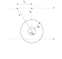
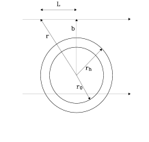
Figure 6: The geometry of a light beam passing a Hernquist lens, indicating the distance of a photon from the centre of the source, $r$, the distance of closest approach, $b$, the radius of the Newtonian bubble, $r_{0}$, and the core radius of the Hernquist profile, $r_{h}$. Top: illustrates situation when $r_{h}<r_{0}$. Bottom: illustrates situation when $r_{h}>r_{0}$.

Figure 7 compares the gravity (solid curves) and Newtonian field strength (plus signs) around a galaxy in a compact Hernquist mass model ($r_{h}=1\,{\rm kpc}$) and an extended Hernquist model ($r_{h}=11\,{\rm kpc}$). For our choice of $\tilde{\mu}$, the scalar field contribution starts at small radii if the gravity $g$ is below $a_{0}$, it then peaks at a value $a_{0}/4$ at a radius $r=2r_{0}-r_{h}$, and then falls to zero again.

Figure 7: The rescaled Newtonian field strength $g_{N}(r)/a_{0}$ (crosses) and rescaled gravity $g(r)/a_{0}$ (solid curves) for an unsmooth function $\tilde{\mu}$ (cf. eq. 12) and a smooth function (cf. eq. 80) around Hernquist models of scale length $r_{h}=1\,{\rm kpc}$ or $11\,{\rm kpc}$ (thin or thick curves) for an elliptical galaxy $M=10^{11}M_{\odot}$. The scalar field contribution ${\bf\nabla}\phi c^{2}/a_{0}$ is $(g-g_{N})/a_{0}$.

Figure 8 compares the radial distribution of the circular velocity for a point-mass and a Hernquist mass distribution in non-relativistic MOND. In the point mass case we see that the velocity curve drops in a Keplerian fashion in the strong, Newtonian limit. At radii beyond the Newtonian bubble radius, the gravity enters the weak MOND-limit, and the velocity flattens to $v=v_{0}$. The size of the Newtonian bubble scales with $M^{1/2}$, and the terminal velocity scales with $M^{1/4}$. The Hernquist models approach the point mass model at large radii; but at small radii, the circular velocity curves are rising instead.

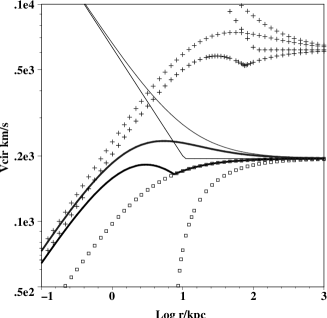
Figure 8: Circular velocity for an elliptical galaxy (lower thick and thin lines) with $M=10^{11}M_{\odot}$ for a point mass model (thin line) and a Hernquist model (thick line) with scale length $r_{h}=3\,{\rm kpc}$ for an unsmooth function $\tilde{\mu}$ (cf. eq. 12) and a smooth function (cf. eq. 80); The boxes show the contribution of the scalar field in these two choices of $\tilde{\mu}$. Likewise for a galaxy cluster with $M=10^{13}M_{\odot}$ (crosses) for a point mass model and a Hernquist model with scale length $r_{h}=30\,{\rm kpc}$. The sharp break point is the transition radius $r_{0}$ from strong gravity to MOND weak gravity.

6.2 Deflection by the Hernquist model

We can now find the reduced deflection angle, $\bar{\alpha}$, for a light beam passing at a radius $\theta=b/D_{L}$ from the Hernquist lens centre. This can again be calculated from equations (27) and (28). Substituting in equation (58) we find

$${\overline{\alpha}\over\theta_{0}\eta^{2}}=\left[{\theta_{0}\theta u+\theta_{0}\theta_{h}H_{0u}\over\theta^{2}-\theta_{h}^{2}}+H_{1u}\right],$$ (63)

where

$$H_{jk}=\cases{{\arcsin(j\sqrt{H})-\arcsin(k\sqrt{H})\over\sqrt{H}},&$H\equiv 1-{\theta_{h}^{2}\over\theta^{2}}\geq 0$,\cr{{\rm arcsinh}(j\sqrt{|H|})-{\rm arcsinh}(k\sqrt{|H|})\over\sqrt{|H|}},&$H<0$\cr}$$ (64)

where

$$u = \sqrt{\left(1-{\theta_{h}\over\theta_{0}}\right)^{2}-{\theta^{2}\over\theta_{0}^{2}}},\qquad|\theta|<\theta_{0}-\theta_{h},$$ (65)

$$= 0\qquad{\rm otherwise}.$$ (66)

The different conditions in equations (64) to (66) correspond to different ray paths through the Hernquist lens, illustrated by Figure 6. For instance, the upper ray on the top panel is outside the Hernquist scale length corresponding to $|\theta|>\theta_{h}$, ie $H>0$, and is also outside the Newtonian bubble, ie $|\theta|>\theta_{0}-\theta_{h}$. This latter condition also requires $\theta_{h}<\theta_{0}$, ie the Hernquist length is smaller than the Newtonian bubble.

The lower ray on the top panel illustrates a different regime, where $|\theta|>\theta_{0}-\theta_{h}$; now the ray passes through the Newtonian bubble, corresponding to the condition given by equation (65).

On the other hand, the bottom panel has $\theta_{h}>\theta_{0}$, ie the Hernquist length is larger than the Newtonian bubble. In this figure therefore, the condition in equation (66) always applies. Nevertheless, the two rays obey the conditions $H>0$ and $H<0$ respectively, as one ray passes through the Hernquist length and one does not.

In summary, the conditions in equation (64) govern whether a ray passes through a Hernquist length of the lens; the conditions in equation (65) and equation (66) govern whether a ray passes within a Newtonian bubble which is larger than a Hernquist length.

In the limit that $\theta_{h}=0$, we find

$$H_{0u}=H_{1u}-{\pi\over 2}=-\arcsin u,~{}u=\cases{\sqrt{1-\left(\frac{\theta}{\theta_{0}}\right)^{2}},&$|\theta|<\theta_{0}$,\cr 0,&$|\theta|>\theta_{0}$,\cr}$$ (67)

which recovers the results for the point-mass (cf. eq. 45).

6.3 Amplification by a Hernquist model

We can find the amplification $A$ for the Hernquist lens from the lens equation

$$A^{-1}={\theta_{s}d\theta_{s}\over\theta d\theta}=\left(1-{\overline{\alpha}\over\theta}\right)\left(1-{d\overline{\alpha}\over d\theta}\right),$$ (68)

where $\overline{\alpha}={D_{ls}\over D_{s}}\alpha$ is given by eq. (63). The amplification diverges when ${d\theta_{s}\over d\theta}=0$ (condition for radial arc) or $\theta_{s}=\theta-\overline{\alpha}=0$ (condition for Einstein ring). In the latter case, the critical radius $\theta_{c}=y_{c}\theta_{0}$ is given by ${\overline{\alpha}\over\theta_{c}}=1.$ Substituting in eq. (63), we have

$${1\over 4\xi}={u_{c}+H_{0u}y_{h}y_{c}^{-1}\over y_{c}^{2}-y_{h}^{2}}+{H_{1u}\over y_{c}},$$ (69)

where $y_{h}\equiv\theta_{h}/\theta_{0}$ and

$$u = \sqrt{\left(1-y_{h}\right)^{2}-y_{c}^{2}}\qquad 1-y_{h}>|y_{c}|$$ (70)

$$= 0\qquad{\rm otherwise},$$ (71)

and $H_{jk}$ is a function of $H=1-\frac{y_{h}^{2}}{y_{c}^{2}}$ as in eq. (64). The above $y_{c}(\xi)$ relation can be used to weigh the lens mass $M$, and hence measure the $M/L$ of the lens. Basically

$$\sqrt{GM\over a_{0}}=r_{0}={\theta_{c}D_{l}\over y_{c}(\xi,y_{h})},~{}\xi={D_{l}D_{ls}a_{0}\over D_{s}c^{2}},$$ (72)

where the lens distance measure $D_{l}$, $\xi$ and the critical line radius $\theta_{c}$ are all observables. In the point mass limit we have $y_{h}=0$, and we find $H=1$, $u=\sqrt{{\rm max}(0,1-y_{c}^{2})}$, $H_{1u}={\pi\over 2}-\arcsin(u)=\arcsin{{\rm max}(1,y_{c})}$, so the critical line satisfies a simpler relation (cf. eq. 50). Note the functional dependence of the rescaled critical radius $y_{c}$ and lens distance measure $\xi$ is fairly complex even with our simplest choice of the free function $\tilde{\mu}$ (cf. eq. 12). It is therefore analytically challenging to work with more general functions for $\tilde{\mu}$.

Figure 5 illustrates how the critical radius increases with the distance parameter $\xi=\eta^{2}/4$ for various values of the Hernquist length scale $r_{h}$; more concentrated models have bigger critical radii, with the biggest in the point mass limit. At small lens distances, we find that the critical radius of an extended Hernquist model can be very small; this is due to the fact that the Hernquist model has a surface density that diverges only logarithmically at small radius. For example, for a very extended Hernquist model with $y_{h}\gg 1\gg y_{c}$, we have $u=H_{0u}=0$, $H\sim-{y_{h}^{2}\over y_{c}^{2}}<0$, $\eta^{-2}=H_{1u}/y_{c}\sim y_{h}^{-1}{\rm arcsinh}{y_{h}\over y_{c}}$. Hence ${\theta_{h}\over\theta_{c}}\rightarrow\sinh\left[\left({GM\over r_{h}^{2}a_{0}}\right)^{-1/2}{D_{0}D_{s}\over 4D_{l}D_{ls}}\right]\gg 1$; the critical radius is relatively small for an extended Hernquist model deep in weak gravity regime where $\left({GM\over r_{h}^{2}a_{0}}\right)\ll 1$, and $D_{0}=c^{2}/a_{0}\gg D_{l}$.

The convergence $\kappa$ and shear $\gamma$ can also be derived analytically; the expressions are somewhat too lengthy to be produced here. Instead we illustrate $\kappa$ and the inverse of amplification $1/A$ as a function of the impact parameter $b$ for a hypothetical example of a Hernquist-profile galaxy cluster lens in Figure (9). Comparing with the point lens case, the convergence is much larger at small impact parameter for the Hernquist case. At very large radius, the Hernquist model approaches the point lens case.

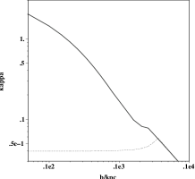
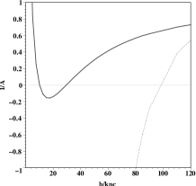
Figure 9: shows two models for a cluster of mass $1\times 10^{14}M_{\odot}$ at $D=0.5$Gpc with a Hernquist scale $r_{h}=100$kpc (solid line) or $r_{h}=0$ (dashed line). Panel (a): Lens convergence $\kappa$. Panel (b): for the inverse of the amplification $\left[(1-\kappa)^{2}-\gamma^{2}\right]$. The Hernquist cluster model is only partly in the weak regime and can create 3 images very close to centre. A radial arc and a tangential arc can form near the critical points at $b=15$kpc and 35kpc for the Hernquist model. Note that the arcs move inwards when going from a point model to Hernquist model.

Table 2: Derived mass ratio $M/M_{*}$ for CASTLES double image lenses. Lens and source redshifts are listed, together with angular diameter distance to the lens and the rescaled lens geometry parameter $\xi$, and lens stellar mass (estimated from evolution and K-corrected I magnitude, except for two systems from R and K magnitudes as indicated by bracket). The lens mass $M$ is calculated using our two techniques (image position and flux ratio) in TeVeS, for both the point mass model and the Hernquist model. For lenses composed of stars of normal stellar populations we expect $M/M_{*}\simeq 1$.

Lens	$z_{l}$	$z_{s}$	$D_{l}$	${D_{l}D_{ls}\over D_{s}D_{0}}$	$M_{*}$	$r_{h}$	${M_{\rm 1,pt}\over M_{*}}$	${M_{\rm 2,pt}\over M_{*}}$	${M_{\rm 1,Hern}\over M_{*}}$	${M_{\rm 2,Hern}\over M_{*}}$
CASTLES			(Mpc)	$=\xi$	$(M_{\odot})$	(kpc)
Q0142-100	0.49	2.72	1190	0.034	$40.8\times 10^{10}$	1.6	0.34	0.19	0.71	0.61
B0218+357	0.68	0.96	1400	0.013	$26.7\times 10^{10}$	-	0.08	0.065	0.35	0.32
HE0512-3329	0.93	1.57	1560	0.019	$556.\times 10^{10}$	-	0.0025	-	0.04	-
SDSS0903+5028	0.39	3.61	1010	0.032	$38.0\times 10^{10}(R)$	-	0.7	0.53	1.10	0.95
RXJ0921+4529	0.31	1.65	880	0.027	$3.36\times 10^{10}$	-	50.7	41.	59.7	50.
FBQ0951+2635	0.24	1.24	730	0.022	$3.09\times 10^{10}$	0.32	0.75	0.35	1.16	0.71
BRI0952-0115	0.41	4.50	1070	0.035	$2.68\times 10^{10}$	0.29	1.3	1.38	1.6	1.7
Q0957+561	0.36	1.41	980	0.027	$84.4\times 10^{10}$	5.23	1.1	0.32	2.8	-
LBQS1009-0252	0.88	2.74	1540	0.032	$9.00\times 10^{10}$	0.80	1.45	1.04	2.24	1.90
Q1017-207	0.78	2.55	1470	0.032	$7.40\times 10^{10}$	1.19	0.53	0.42	1.19	1.49
B1030+071	0.60	1.54	1320	0.027	$16.6\times 10^{10}$	1.50	0.45	0.23	1.45	1.8
HE1104-1805	0.73	2.32	1440	0.032	$33.2\times 10^{10}$	2.48	2.1	1.23	3.0	1.9
SDSS1155+6346	0.18	2.89	540	0.020	$4.40\times 10^{10}(K)$	-	.43	-	3.8	-
SBS1520+530	0.72	1.86	1430	0.028	$28.0\times 10^{10}$	1.32	0.57	0.33	0.96	0.72
B1600+434	0.41	1.59	1070	0.029	$4.00\times 10^{10}$	-	1.9	1.13	4.3	3.5
PKS1830-211	0.89	2.51	1540	0.031	$14.8\times 10^{10}$	-	0.5	0.94	1.1	1.7
HE2149-2745	0.50	2.03	1200	0.032	$20.0\times 10^{10}$	11.4	0.5	0.29	6.0	-
SBS0909+523	0.83	1.38	1506	0.019	$655.\times 10^{10}$	-	0.03	0.02	0.05	0.04

7 Comparing TeVeS predictions to galaxy lens data

7.1 Stellar mass of the CASTLES sample

Now that we have developed models for lensing by point masses and Hernquist profile lenses, we will apply this formalism to galaxy lens observations. In particular, we will examine the consistency of the strong lensing predictions for galaxy lenses in the CASTLES survey (CfA-Arizona Space Telescope Lens Survey; Munoz et al 1999).

Here we use galaxies with known double/quadruple lensed quasars, with critical lines estimated from the quasar separation, baryonic mass inferred from luminosity, and known redshifts from the CASTLES sample (Kochanek et al, 2000). In the spirit of TeVeS all of the lensing galaxies have $M/L$ of order unity. However, to be rigourous, we must include the K-correction, the luminosity evolution with redshift, and the possibility of significant gas and extinction from dust.

Kochanek et al (2000, Table 6) have measured combined K-correction and evolution corrections for CASTLES lenses, and find a correction for the $I$ band which varies with redshift ($0.36<z<0.88$ as appropriate for most of our lenses, a low density open universe with $\Omega_{0}=0.3$) corresponding to a $\simeq 11$ percent mean offset in luminosity, which will not impact significantly on our conclusions about whether TeVeS provides reasonable mass-to-light ratios.

To make the interpretation of our lens model more direct, we first estimate the stellar content of the high-z lens using its observed I-magnitude and a model for the spectral energy distribution of an old non-evolving stellar population. We first estimate the luminosity without K-correction, or evolution/reddening correction by

$$L=\left({D_{A}(z)(1+z)^{2}\over 10\,{\rm pc}}\right)^{2}10^{0.4(m_{\lambda_{0},\sun}-m_{\lambda_{0},obs})},$$ (73)

where $D_{A}(z)$ is the angular diameter distance to the lens, $(1+z)^{4}$ gives the dimming effect, $m_{\lambda_{0},\sun}$ is the $\lambda_{0}$-band magnitude of the Sun. We then estimate the stellar mass by the simple formula

$${M_{*}\over M_{\odot}}=\gamma\left({\lambda_{0}\over 1+z}\right)\times L,\qquad\gamma\left({\lambda_{0}\over 1+z}\right)=\gamma(\lambda_{0})10^{0.4\gamma_{1}z},$$ (74)

where $\gamma\left({\lambda_{0}\over 1+z}\right)$ is the estimated mass-to-light ratio of a typical nearby elliptical galaxy observed at the emitting wavelength ${\lambda_{0}\over 1+z}$; e.g., observations at I-band $\lambda_{0}=8140A$ corresponds to light emitting at $z=0.5$ with a rest-frame wavelength ${\lambda_{0}\over 1+0.5}=5000A$, approximately the V-band. The parameter $\gamma_{1}$ parametrizes the countering effects of the K-correction, and the passive evolution/extinction after starbursts; these effects tend to cancel each other for most cosmologies and reasonable formation redshift of ellipticals, and models with very late/very early formation ellipticals give $\gamma_{1}>0$ and $\gamma_{1}<0$ respectively (see Fig.8 of Kochanek et al. 2000). For the I-band we set

$$m_{8140A,\sun}=4.1^{m},\qquad\gamma(8140A)=4{M_{\odot}\over L_{\odot}},\qquad\gamma_{1}\approx 0.$$ (75)

This is calibrated using Fig.32 of Worthey 1994, assuming a 12-Gyr old solar metallicity stellar population; while the I-band luminosity of a 12-Gyr old red elliptical galaxy is more than its V-band luminosity, it is actually comparable to the rest-frame V-band luminosity of its 5-Gyr old younger counterpart at $z=0.5$. For three of our lenses without I magnitude, we use the nearest available band R, H, V or K magnitude. We make similar conversions of mass to light using Worthey models for these bands, and checked against the predicted redshift dependence of the lens galaxy colours $V-I$, $R-I$, $I-H$ with those in the literature (cf. Fig.4 of Keeton et al. 1998, Fig. 1 of Kochanek et al. 2001).

Galaxies tend to be more dusty and gas rich at higher redshift. Falco et al. (1999) found that a rest-frame differential reddening $\Delta E(B-V)\sim 0.07^{m}-0.1^{m}$ on average for 23 lenses (mostly early-type galaxies). McGough et al (2005) have compiled extinction for 25 CASTLES lenses (see their Table 1); the extinction observed at I-band of most lenses is $\Delta A_{I}\sim{5550A\over 8140A(1+z)^{-1}}\times 3.1\Delta E(B-V)\sim 2(1+z)\Delta E(B-V)\leq 0.8^{m}$, i.e., less than a factor of two correction of the luminosity. Note that we exclude five lenses with $\Delta E(B-V)>0.4/(1+z)$, which are mainly high redshift late-type lenses. The consensus seems to be that gas and dust play insignificant roles in elliptical galaxies in general, and there is strong evidence against a large dust lane for a lens at $z=0.84$ (Kochanek et al. 2000b). In any case, only the far side of a spherical lens galaxy is affected by the dust lane, hence the dust effect on the total luminosity is likely mild, less than a factor of two.

7.2 Critical lines and lens geometry test

Now we compare the predicted position of critical radii in TeVeS with CASTLES data. Figure 5 shows the predicted scaling of the critical line opening angle, $y_{c}=\theta_{c}/\theta_{0}$, with the lens geometry factor, $\xi=\eta^{2}/4$. It is interesting that the range of galaxies in this survey all lie in the strong-gravity regime, where $\xi\ll 1$. This is due to the fact that the angular diameter distance in a TeVeS universe has a maximum value which is much smaller than the $D_{0}$ scale of TeVeS (cf. Fig.3). Therefore all of the lenses in the sample have a small $\xi$, and are never in the purely weak gravity regime. This ”coincidence” is actually a natural consequence of the small value for $a_{0}$. has also been anticipated by Sanders (1999), who noted in passing that MOND effects become important below a threshold in the surface density of a galaxy cluster, while the minimal surface density of image-splitting galaxy clusters is always above this MOND threshold. Hence the deep-MOND effect is argued to be small.

Secondly we note that the mean position of galaxies in the plot lie on the point-lens prediction. This appears to be a success for TeVeS, where the stellar mass can produce reasonable size Einstein rings. On the other hand real galaxies are not point masses. Furthermore there are many galaxies which are outliers in this distribution; this scatter in lens bending power is not expected in a TeVeS universe, as the displayed TeVeS predicted curve should be universal if galaxies can be approximated as point lenses.

Thirdly the scatter of observed lenses cannot be explained by extending the lens via a Hernquist model. As shown in Figure 5, Hernquist models have lower bending power, and so cannot explain the images with large separation.

7.3 Double image lenses

We now conduct a more detailed study of double-image image lenses from the CASTLES survey in the context of TeVeS theory with the point and Hernquist models. Here we examine only lenses with almost co-linear double images, as non-co-linear images and quadruples cannot be modelled in detail by our spherical models.

Figure 10: Upper panel: The TeVeS lens mass for $Q0142-100$ using the image position technique; here we assume a point mass lens model. The two curves represent the permitted mass and source position for the two images; their intersection provides a unique consistent TeVeS mass for the object. Lower panel: The TeVeS lens mass for $Q0142-100$ using the image position technique, with Hernquist scale length of 1.6kpc.

Figure 11: The TeVeS lens mass for $Q0142-100$ using the flux ratio technique, with a point mass model. The curve represents the permitted mass and flux ratio for the two images; the straight line provides the measured flux ratio. The intersection provides a determination of the TeVeS mass for the object. Lower panel: The TeVeS lens mass for $Q0142-100$ using the flux ratio technique, with Hernquist scale length of 1.6kpc.

7.3.1 Source position method

We determine the lens mass by two methods. The first is by inverse ray tracing, i.e. from one of the image positions we can predict the source position as a function of lens mass, using e.g. equation (24). By matching source positions from both images, we therefore measure the mass according to the TeVeS/MOND theory.

An illustration of this technique is given in Figure 10 for CASTLE lens $Q0142-100$. This system includes two images at angular distances 1.9” and 0.4” from the lens, with source redshift 2.72 and lens redshift 0.49. In the figure we see that, for a TeVeS point-mass, we can calculate predictions for the real, pre-lensed angular position of the source as a function of mass for each of the two images; where these predictions intersect we have a unique measurement of the lens mass, which is here found to be $M=(1.38\pm 0.002)\times 10^{11}M_{\odot}$.

The exercise can be repeated with a finite Hernquist scale-length $r_{h}$ for the lens. The bottom panel of Figure 10 demonstrates that the resulting mass estimate is quite sensitive to $r_{h}$; for a scale length of 1.6kpc for our lens galaxy, the mass estimate is increased to $(2.86\pm 0.004)\times 10^{11}M_{\odot}$. In order to find $r_{h}$ in each case, we use the half light radius for the galaxy, $r_{e}$ as given for CASTLES lenses by Kochanek et al (2000) and using the relation of Hernquist (1991), $r_{h}=r_{e}/1.82$ to relate $r_{e}$ to $r_{h}$.

7.3.2 Flux ratio method

The second method of measuring lens mass is to predict an amplification map on the image plane as a function of mass. This can be achieved by calculating the rate of change of deflection angle $\alpha$ with the image position $\theta$ as a function of mass. From this one can calculate the rate of change of apparent position with respect to the unlensed source position $\theta_{s}$, hence the flux ratio of two images is predicted by

$${A_{1}\over A_{2}}=\frac{\theta_{1}}{\theta_{2}}\left({1-\frac{\partial\alpha_{1}}{\partial\theta_{1}}\frac{D_{LS}}{D_{S}}\over 1-\frac{\partial\alpha_{2}}{\partial\theta_{2}}\frac{D_{LS}}{D_{S}}}\right)^{-1}.$$ (76)

Figure 11 shows this predicted ratio as a function of mass for the example double-image lens $Q0142-100$, for a point-mass TeVeS model; also shown is the empirical flux ratio between the two lenses. We find that the TeVeS mass consistent with the observed flux ratio is $(7.8\pm 0.09)\times 10^{10}M_{\odot}$. This is similar in magnitude to the mass found from the source position method above, but is clearly not consistent with it in detail. In order to obtain consistency, one requires a Hernquist model with $r_{h}=2.3$kpc. In contrast, the value of $r_{h}$ expected from half-light measurements is 1.6kpc, so modelling the extended nature of the lens mass cannot be used to account for all of the difference between the two estimates. One may see this as a potential difficulty for TeVeS; alternatively we should note the simplicity of the model we are using (spherically symmetric, specific profile) which may account for some or all of the 43% difference between the two estimates.

The bottom panel of Figure 11 shows the equivalent test with the measured $r_{h}=1.6$kpc; in this case we find a TeVeS mass of $(2.52\pm 0.03)\times 10^{11}M_{\odot}$. In this case, the mass is closer in magnitude to the TeVeS mass found via the image position technique ($\simeq 13$% difference), but is not consistent in detail; again, the simplicity of the lens model may be the cause of this.

7.3.3 Results for CASTLES lenses

We have applied the two TeVeS mass estimation techniques to a set of double image lenses from the CASTLES survey (Table 2), for both point mass and Hernquist models. The lenses were selected to have known redshifts for source and lens, known magnitudes in F814, and to have only two images. We examine the TeVeS mass of these lenses in relation to their absolute luminosity (from F814 magnitude) in Figure 12, for point lens and Hernquist lens cases with the position method. Seven of the lens galaxies do not have published half-light radii; for these we ascribed the median Hernquist length of the galaxies with known radii, $r_{h}=1.8$kpc.

We note that there is an apparent correlation between the TeVeS mass and the luminosity in the F814 band in both the point and Hernquist cases; this is broadly consistent with TeVeS, which predicts a strong correlation between mass and luminosity. However, there are some very significant outliers, leading to a negative Pearson’s correlation coefficient (-0.12 for point-mass; -0.04 for Hernquist).

Finally we can derive the ratio of lens mass vs. stellar mass for each galaxy, using lens masses from either the position method or flux ratio method. In Figure 14 we show the mass-to-mass ratios $M_{\rm lens}/M_{*}$ from both of these methods, using the Hernquist model.

Three points of interest arise from this plot. Firstly, we note that the mass-to-$M_{*}$ ratios calculated using the two independent methods closely agree, i.e. $(M/M_{*})_{\rm Flux}\simeq(M/M_{*})_{\rm position}$. This shows that TeVeS is working well in terms of being a theory which appropriately includes gravitational lensing; if there were not a good level of agreement, it would suggest that different lensing predictions were not consistent in TeVeS. As it is, TeVeS is obtaining consistent results from lensing distortions of position and magnifications. Nevertheless, for several lenses, e.g., SDSS1155+6346, the flux ratio cannot be reproduced with any lens mass, hence the empty entries in Table 2. This might reflect the fact that the flux ratios have been perturbed by microlensing or substructures. Overall the source position method is more reliable than the flux ratio method.

The second point concerns the TeVeS mass and absolute luminosity for both point and Hernquist models. There is a strong correlation between the point and Hernquist mass estimations themselves (see Figure 13). We can see that point lens models underpredict the required baryonic mass for a given set of image positions in relation to the Hernquist model, by a mean factor of 3.6. This confirms the value of extending our analysis to the Hernquist model.

The third point of interest from this plot concerns the range of mass-to-$M_{*}$ ratios measured. All but two of the lenses are found to have $M/M_{*}$ between 0.5 and 2; this is a reasonably concentrated distribution. However, we note the existence of extreme outliers such as RXJ0921+4529 with $M/L=239$ and HE0512-3329 with $M/L=0.16$ (cf. Table 2 for the mass ratio $M/M_{*}$).

Figure 12: Upper panel: TeVeS lens mass for double image CASTLES lenses using the image position technique (point mass), as a function of (converted) F814 absolute luminosity for these lenses. The lines indicate $M/L=4$ (dashed). Lower panel: TeVeS lens mass for double image CASTLES lenses using the image position technique (Hernquist), as a function of F814 absolute luminosity for these lenses. Open circles show lenses where the median Hernquist length has been used; for easy comparison, these lenses are also displayed with open circles in the upper panel, where Hernquist length is irrelevant. Note five outliers indicated by five open diamonds.

Figure 13: Comparison of TeVeS masses obtained using the image position technique, for point masses and Hernquist models. The dotted line indicates equality of mass; open circles show lenses where the median Hernquist length has been used.

Figure 14: The lens mass to stellar mass ratio $M/M_{*}$ from two methods for Hernquist profiles using realistic length scales. The dotted line indicates equal mass-to-light ratios; open circles show lenses where the median Hernquist length has been used. The data are expected to be tightly clustered around $M/M_{*}\sim 1$ in MOND/TeVeS.

8 Discussion

8.1 RXJ0921+4529

As noted in the last section, there are several lenses with anomalous $M/L$. In particular the galaxy RXJ0921 with luminosity $L=0.84\times 10^{10}L_{\odot}$ requires either a point mass of $1.7\times 10^{12}M_{\odot}$ or a Hernquist profile mass of $2.0\times 10^{12}M_{\odot}$. This lens is therefore required to have a $M/L\sim 240$, which could seriously challenge the TeVeS theory.

Nevertheless, several explanations are initially available in defence of TeVeS for this system. The first possibility is that this lens is severely dimmed by obscuration of dust; however, the $I-H$ colour of the lens appears normal, which would not be expected in the presence of dust.

Muńoz et al. (2001) also note an extended emission source B’ offset from the B image for this system, and there is no extended counterpart in the image A. An important although unlikely explanation is that A and B are a pair of independent quasars with small separations and the same redshift, and the quasar B is off-centred from its host galaxy B’ as well. A more plausible explanation is that B’ is a member galaxy in the same cluster, projected by chance near one of the two split images of a lensed quasar.

Another suspicion would be that this outlying mass is due to the use of too large a Hernquist length (as this is a lens where the median $r_{h}$ is used); however, the fact that the large mass is found even in the point-mass case allays this concern.

Yet another possibility for the high M/L is the fact that the lens sits in the middle of an X-ray cluster; this will increase the lensing distortion associated with the system. This issue clearly requires follow-up using lens models more sophisticated than those considered in this paper, which would be able to model multi-component lenses with different length-scales.

Another system with a mildly high $M/L$ is B1600+434; however, unlike our other lenses this is found to be an edge-on spiral galaxy. A Hernquist model will not provide a good fit to the baryonic matter in a spiral, so it is unsurprising that this $M/L$ is an outlier. Indeed, with a point mass model, the mass-to-light is more reasonable (4.5 or 7.5).

In summary, at least one outlier in our study succeeds in overcoming some of the defences available to TeVeS; however, the presence of a lensing cluster does call into question the level of disagreement between TeVeS predictions and data on this lens.

8.2 Effects of different choices of $\tilde{\mu}$ and $a_{0}$

One concern regarding the above result is that we used an unsmooth function $\tilde{\mu}$ (cf. eq. 61), which reduces the contribution of the scalar field to exactly nothing in the strong gravity regime. Since most lenses have impact parameters inside the Newtonian bubble, letting the scalar field contribute in the strong gravity could help towards the $M/L$ discrepancy. Common choices of $\tilde{\mu}$ include

$$\tilde{\mu}=\cases{{g/(g+a_{0})}\cr{g/\sqrt{g^{2}+a_{0}^{2}}}\cr 1-\exp(-g/a_{0}).\cr}$$ (77)

Another concern is that $a_{0}$ could be slightly (by a factor of two in some systems) higher than $1.2\times 10^{-8}{\rm cm}{\rm s}^{-2}$ given reasonable errors on disk galaxy rotation curve (RC) data (Sanders & McGaugh 2002).

To address these concerns we consider a new smooth function $\tilde{\mu}$ so that

$$\delta_{\phi}={{\bf\nabla}\phi c^{2}\over a_{0}}={\tilde{\mu}\over 1-\tilde{\mu}}$$ (78)

is a monotonic increasing function of $\tilde{\mu}$, closely matching that chosen by Bekenstein (cf. eq. 13, as illustrated in Fig. 1).

With a bit of algebra it can be shown that

$$g=g_{N}+{\bf\nabla}\phi c^{2}=g_{N}+\sqrt{g_{N}a_{0}},$$ (79)

and

$$\tilde{\mu}={\delta_{\phi}\over 1+\delta_{\phi}}={a_{0}\over 4g}\left[\sqrt{1+{4g\over a_{0}}}-1\right]^{2}.$$ (80)

The gravity and rotation curve of a Hernquist galaxy or galaxy cluster in such a model are shown in Fig. 7 and  8. The curves are much smoother than those in our principal model. Here the scalar field contributes even inside the Newtonian bubble (strong gravity regime), unlike that in our principal model. Also this model and our earlier choice of $\tilde{\mu}$ bracket all common choices of $\tilde{\mu}$ (cf. Fig. 15).

Figure 15: The MOND/TeVeS functions $\tilde{\mu}$ and $\delta_{\phi}$ (shifted down by a factor of 10). Common choices of $\tilde{\mu}$ are shown in symbols, which are bracketed by our choices (thin and thick solid curves). All these choices converge asymptotically so that $\tilde{\mu}\rightarrow\delta_{\phi}\rightarrow g/a_{0}$ in the weak gravity regime (below the horizontal dashed line).

Interestingly, our new choice of $\tilde{\mu}$ also allows the deflection of Hernquist lens model to be calculated analytically, and we find that the rescaled critical radius $y_{c}$ satisfies

$${y_{c}\over 4\xi}=\left[{y_{c}-y_{h}H_{10}\over y_{c}^{2}-y_{h}^{2}}+H_{10}\right],~{}H_{10}={\arcsin\sqrt{1-{y_{h}^{2}\over y_{c}^{2}}}\over\sqrt{1-{y_{h}^{2}\over y_{c}^{2}}}},$$ (81)

where

$$\xi={a_{0}\over c^{2}}{D_{l}D_{ls}\over D_{s}},~{}y_{c}=D_{l}\theta_{c}\sqrt{a_{0}\over GL}(M/L)^{-1/2}.$$ (82)

This allows us to estimate the lens mass $M$ by fitting the Einstein ring size; the solution has to be found by iteration because eq. 82 is an implicit non-linear function of $M/L$ through $y_{c}$ and $y_{h}$.

Table 3: CASTLES lenses with anomalously large/small ${M_{\rm lens}\over M_{*}}$.

Lens	Comments
RXJ0921+4529	2-image. Resides in cluster
SDS1004+4122	2-image. Resides in cluster
B1600+434	2-image. Edge-on spiral lens with dust lane
MG2016+112	3-image. One or two lens planes
B2045+265	4-image. Source near cusp caustic
HE0512-3329	2-image. Gas-rich lens.
SBS0909+532	2-image. Early-type, little gas/dust
B0218+357	2-image. Lens is likely a spiral galaxy.
RXJ1131-1231	4-image. V-magnitude. Cusp caustic. Elliptical.
B1933+503	10-image components. Fits $R^{1/4}$-law.

8.3 Constraints on $\tilde{\mu}$ from a larger sample

Fig. 16 shows the application to a sample similar to those shown in Fig. 5, including all CASTLES double/four-imaged lenses with measured lens and source redshifts. Note the very large scatter overall. There are galaxies well above and well below the expected stellar mass, which cannot be simply explained by extinction, evolution or K-correction. Interestingly, SDSS1004+4122 is also in a galaxy cluster (from which the lens redshift was assigned), similar to the situation of RXJ0921+4529. At the opposite end, the lens galaxy of HE0512-3329 is a gas-rich damped Lyman absorber galaxy, barely resolved at $z=0.93$ with a size $\sim 1\,{\rm kpc}$ comparable to the resolution of the Hubble Space Telescope (Gregg et al. 2000). Nevertheless, the stellar mass alone seems to exceed what is required for lensing. A similar situation pertains to SBS0909+532, an early type lens without much gas and extinction (Lubin et al. 2000, McGough et al. 2005). Some features of these outliers are compiled in Table 3.

Selecting only a well-behaved subsample (e.g., excluding disky and/or dusty galaxies, galaxies with unknown half-light radius and/or unknown magnitude), we find that the scatter is still significant, with especially large deviations for three high redshift lenses. The $M_{\rm lens}/M_{*}$ shows mild dependence on the lens redshift $z_{l}$, suggesting the need for K-correction. To make $M_{\rm lens}/M_{*}\sim 1$ for the $z=0.9-1.0$ lenses would require a model where $\gamma(\lambda_{z})$ increases by one decade (i.e., $\gamma_{1}=2.5^{m}$) per unit redshift; this is too steep even for purely K-corrected models where galaxies do not evolve (dashed line, taken from Fig.8 of Kochanek et al. 2000). While it has been suggested before that MG2016+112 might involve two lenses at two redshifts (Nair & Garrett 1997), a more recent model found that a single lens plane is sufficient (Koopmans et al. 2002). The early type (Sa) lens B2045+265 from the CLASS survey seems to be a robust case of a single lens with accurate NICMOS near IR data and radio data; the source is near a cusp caustic, and is split into three images on one side and one image $2\arcsec$ away on the other side of the resolved lens (Fassnacht et al. 1999). The peculiar flux ratios in both radio and near IR among the three images near the critical curve have been used to highlight the existence of dark substructures (Keeton et al. 2003).

Another way of describing the residue between mass and light is by using the theoretically uncertain modification function $\tilde{\mu}$. We slide the function $\tilde{\mu}$ in between two expressions, say $\tilde{\mu}_{1}$ and $\tilde{\mu}_{2}$, which are that of equation (12) and that of equation (80) respectively by making the linear combination

$${1\over\tilde{\mu}}={f\over\tilde{\mu}_{1}}+{1-f\over\tilde{\mu}_{2}},\qquad-\infty<f<1.$$ (83)

The results with a slidable $0<f<1$ are shown as the upper thick part of the error bars in Fig. 16. Still we find $M_{\rm lens}/M_{*}\neq 1$ for many systems. Model with $f<0$ seems necessary.

Yet another possibility is that the value for $a_{0}=a_{0}^{RC}=1.2\times 10^{-8}{\rm cm}{\rm s}^{-2}$ from disk galaxy rotation curve (RC) measurements could be an underestimate. Larger values have been suggested in galaxy cluster studies (e.g., Pointecouteau & Silk 2005 and Sanders & McGaugh 2002). So suppose the theoretical value for

$$a_{0}=(1,2,4,8)\times a_{0}^{RC}=(1.2,2.4,4.8,9.6)\times 10^{-8}{\rm cm}{\rm s}^{-2}.$$ (84)

Keeping $\tilde{\mu}$ as in eq. (80), adopting bigger $a_{0}$ has the effect of lowering $M_{\rm lens}/M_{*}$ (shown by the lower segments of the error bars). Nevertheless, a good match to $M_{\rm lens}/M_{*}\sim 1$ still seems difficult. A few systems seem to suggest an $a_{0}$ more than factor of 10 higher than the standard value $a_{0}^{RC}$ from rotation curves of disk galaxies. In short, the recurring discrepancy between some lenses and MOND/TeVeS predictions seems to go beyond the simplest lens models, and remains with many plausible functions of $\tilde{\mu}$ and plausible values for $a_{0}$.

A related point is that not all popular MOND $\tilde{\mu}$ correspond to a plausible Lagrangian for the scalar field. Zhao & Famaey (2005) noted that the standard function $\tilde{\mu}(g/a_{0})=g/\sqrt{a_{0}^{2}+g^{2}}$ makes the gravity $g$ (and all its functions) multi-valued for the same strength of the scalar field. This happens for all sharply increasing $\tilde{\mu}$, including our principal one (see Fig. 15). These models are perhaps undesirable since the scalar Lagrangian cannot be expressed uniquely by the scalar field strength. The lensing predictions of TeVeS are likely in a range narrower than depicted by the ”error bars” in Fig. (16).

Figure 16: Shows the lens redshift-dependence of the mass ratio $M_{\rm lens}/M_{*}$ derived from fitting the Einstein ring size of the CASTLES sample (circles). Circles with error bars are for well-behaved subsample of CASTLES lenses which have the Hernquist profile and little dust/gas. The upper thick part of an error bar brackets the range of uncertainty of the modification function $\tilde{\mu}$ (as shown in Fig. 15) for fixed $a_{0}=a_{0}^{RC}=1.2\times 10^{-8}{\rm cm}{\rm s}^{-2}$. The lower part of an error bar with alternating thickness adopts $a_{0}=(1-2)a_{0}^{RC},(2-4)a_{0}^{RC},(4-8)a_{0}^{RC}$ but fixes $\tilde{\mu}$ as in eq. 80. Circles with central asterisks are lenses with unresolved scale-length (adopt $1.82\theta_{h}=0.1\arcsec$). Circles with smaller circles are very faint lenses with unknown magnitude and scale-length (adopt $I=21^{m}$ and $1.82\theta_{h}=0.1\arcsec$). The solid horizontal line is the expected K-corrected value (unity) for plausible star formation and passive evolution of ellipticals. The dashed line shows the expected K-corrected value but assuming galaxies do not evolve.

9 Conclusion

We have explored key properties of gravitational lensing as it occurs in Bekenstein’s theory TeVeS, a fully covariant modified gravity theory. We have shown that TeVeS is frequently successful in predicting gravitational lensing phenomena; however, there are lens systems where TeVeS appears to fail radically.

We began by giving an account of TeVeS theory. Lensing is still governed in TeVeS by a gravitational potential $\Phi$ which enters the metric in a similar way to General Relativity. However, the interpretation of the gravitational potential is different; rather than this being due to baryonic and dark matter, it is solely due to baryonic matter, which generates a gravitational potential in excess of the GR prediction. The usual relations among lensing deflection angle, the lens equation, convergence, shear and magnification still hold except that their values as functions of the impact parameter have changed, as we have shown analytically for point-mass lens. E.g., the convergence of a point-mass lens is non-zero in TeVeS. Analytical lens models are also constructed for a Hernquist profile, which should be a good model for baryons in most elliptical galaxies. Conditions for generating arcs are discussed appertain to galaxy cluster scales.

We then further tested the theory using galaxy lens data from the CASTLES survey. We find that the observed relationship between critical lines and lens geometry (cf. Fig. 5) would be largely consistent with TeVeS if lenses were treated as point-lenses, but there are a handful of outliers. We also calculated TeVeS masses for CASTLES double-image lens galaxies, assuming point mass lenses or Hernquist lenses, and using image positions or fluxes to calculate mass. We found that TeVeS/MOND provides an acceptable explanation for the lensing data in general. But in a handful of cases we obtain too large or too small mass-to-light ratios (cf. Fig. 14, Fig. 16, and Tables 2-3). Another way to put this is that we observe some cases of deviations from the expected baryonic content; or the $a_{0}$ derived from the critical lines of some individual galaxies deviates markedly from the TeVeS/MOND expectation (cf. Fig. 16). More detailed photometric and spectroscopic data of these outlier lenses (see Table 3) are needed urgently to clarify the degree of the problem.

On cosmology in the TeVeS context we noted the likely need for a cosmological constant (allowed in both TeVeS and GR). If $\Omega_{\Lambda}\sim 0.46$ it is possible to construct a low density baryonic universe that agrees with current cosmological constraints from supernovae and which equivalently provides an acceptable angular diameter distances at low redshifts. Such an open cosmology might not be the best for TeVeS since the sound horizon size at the last scattering is underpredicted. (cf. Fig. 3).

This work has made initial tests of TeVeS using gravitational lensing. Our analysis of TeVeS in the weak field regime suggests that our results might be valid for any relativistic theory that asymptotes to MOND in the weak field regime. Further refinement of these tests (Shan et al. 2006) will involve examining non-circular TeVeS lenses to ascertain whether they fit the double and quadruple imaged lenses in more detail. Observed time delays between images of a dozen systems could also be constraining (Zhao & Qin 2005). Further work will also extend the analysis to a wider range of density profiles, including the beta-profile most suitable for analysing cluster lensing. In the meantime, we see that TeVeS succeeds in providing an alternative to General Relativity in some lensing contexts; however, it faces significant challenges when confronted with particular galaxy lens systems. Finally, we see that gravitational lensing can be used as a useful approach to distinguish between theories of gravity, and to probe the functional form of the modification function $\tilde{\mu}$. In the mixed model (cf. Eq. 83) the gravity $g$ rises more steeply with $\tilde{\mu}$ for models with smaller $f$ and even negative $f$ (cf. Figure 15). E.g., the model with $f=0$ (Bekenstein 2005) is more effective in bending light for the same baryonic mass than models with $\tilde{\mu}=x/(1+x)$, $\tilde{\mu}=x/\sqrt{1+x^{2}}$, $\tilde{\mu}=\min(1,x)$ (cf. Figure 16). The model with $f=0.5$ mimics the simple function $\tilde{\mu}=x/(1+x)$ in the intermediate regime. Any model with $f>0.5$ is only only inefficient in lensing, but also always shows an undesirable peak in the scalar field strength $\delta_{\phi}^{2}$. This leads to unphysical external field effect according to Zhao & Famaey (2005). They also find that models with $f\leq 0$ have a wide transition zone, which do not fit the sharply rising rotation curves seen in galaxies. Putting all these constraints together, it seems that the MOND/TeVeS models with $0\leq f\leq 0.5$ have the best chance to survive.

References

- [1] Bartelmann M., Schneider P., Phys. Rep. 340, 291.
- [2] Bekenstein J. 2004, Phys. Review D., 70, 3509
- [3] Bekenstein J. & Milgrom M. 1984, ApJ, 286, 7,
- [4] Binney J. & Tremaine S., 1987, Galaxy dynamics, Princeton University Press.
- [] Chiu M., et al. 2005, ApJ, in press, astro-ph/0507332
- [5] Ciotti L., Binney, J. 2004, MNRAS, 351, 285
- [6] Fassnacht C.D. et al. 1999, AJ, 117, 658
- [7] Falco E.E. et al. 1999, ApJ, 53, 617
- [8] Famaey B. & Binney J. 2005, MNRAS, in press
- [9] Gregg M.D. et al. 2000, ApJ, 119, 2535
- [10] Hernquist L., 1990, ApJ, 356, 359
- [] Hao J. & Akhoury R. 2005, astro-ph/0504130
- [11] Keeton C., Gaudi S., Petters A.O., 2003, ApJ, 598, 138
- [12] Kochanek C. et al, 2000, ApJ, 535, 692
- [13] Kochanek C. et al, 2000, ApJ, 543, 131
- [14] Kochanek C., 2003, ApJ, 583, 49
- [15] Koopmans L. et al. 2002, MNRAS, 334, 39
- [16] Lubin L. et al. 2000, AJ, 119, 451
- [17] McGough C., Clayton G.C., Gordon K.D., Wolff M.J. 2005, ApJ, 624, 118
- [18] Milgrom M. 1983, ApJ, 270, 365
- [19] Milgrom M., 1986, ApJ, 302, 617
- [20] Milgrom M. , Sanders R. H. 2003, ApJ, 599, L25,
- [21] Munoz J.A., Kochanek C., Falco E.E., 1999, Astrophys. Space Sci. 263, 51.
- [22] Mortlock D., Turner, E.L., 2001, MNRAS, 327, 557
- [23] Nair S. & Garrett M. 1997, MNRAS, 284, 58
- [24] Percival W., et al., 2002, MNRAS, 337, 1068
- [25] Perlmutter S., et al., 1999, ApJ, 517, 565
- [] Pointecouteau E., & Silk J., 2005, MNRAS, in press, astro-ph/0505017
- [26] Qin B., Wu, X.P., Zou Z.L., 1995, A&A, 296, 264
- [27] Refregier R., 2003, ARA&A, 41, 645.
- [28] Riess A., et al., 1998, AJ, 116, 1009
- [29] Romanowsky A. J. et al. 2003, Science, 301, 1696
- [30] Sanders R., 1999, ApJ, 512, L23
- [31] Sanders R., 2003, MNRAS, 342, 901
- [32] Sanders R., 2005, MNRAS, 363, 459
- [33] Sanders, R. , McGaugh S. 2002, ARA&A, 40, 263,
- [] Shan H.Y., et al., 2005, in prep.
- [] Skordis C. et al., 2005, Phys. Rev. Lett. in press, astro-ph/0505519
- [34] Spergel D., et al., 2003, ApJSupp, 148, 175
- [35] Tegmark M., et al., 2004, Phys. Rev. D, 69, 103501
- [36] Van Waerbeke L., Mellier Y., astro-ph/0305089.
- [37] Worthey G., 1994, ApJS, 95, 107
- [] Zhao H., 2005, A&A Letters, 444, L25
- [] Zhao H., & Famaey B., 2005, ApJ, submitted (astro-ph/0512425)
- [] Zhao, H. S., Pronk, D., 2001, MNRAS, 320, 401
- [] Zhao H., Tian L., 2005, A&A, submitted
- [] Zhao H., & Qin B., 2005, ChJAA, accepted