Galaxy number counts – VI. An $H$-band survey of the Herschel Deep Field

Abstract

We present $H$-band infra-red galaxy data to a $3\sigma$ limit of $H\sim 22.9$ and optical-infra-red colours of galaxies on the William Herschel Deep Field (WHDF). These data were taken from a $7^{\prime}\times 7^{\prime}$ area observed for 14 hours with the $\Omega$ Prime camera on the 3.5-m Calar Alto telescope. We also present counts derived from the HDF-S NICMOS camera to the limit of $H\sim 29$ mag over a $0.^{\prime}95\times 0.^{\prime}95$ area. Following previous papers, we derive $H$-band number counts, colour-magnitude diagrams and colour histograms for the whole $H$ selected sample. We review our Pure Luminosity Evolution (PLE) galaxy count models based on the spectral synthesis models of Bruzual & Charlot. We find that our previously assumed forms for the luminosity function agree well with those recently derived from 2dFGRS/2MASS at $B$ and $K$, except that the 2dFGRS $K$ LF has an unexpectedly flat slope which, if correct, could affect our interpretation of the faintest $H$ and $K$ counts.

We find that these PLE models give an excellent fit to the WHDF $H$ band count data to $H<22.5$ and HDF count data to $H<28$. However, if we use the flat 2dFGRS/2MASS near infra-red (NIR) LF then the predicted count is too flat at $H>21$. We confirm that PLE models that assume a Salpeter IMF for early-type galaxies overestimate the average galaxy redshift in $K<20$ galaxy redshift surveys. Models that assume a steep $x=3$ IMF continue to give better agreement with the $N(z)$ data than even models based on a Scalo IMF, although they do show an unobserved peak in $B-H$ and $I-H$ colour distributions at faint $H$ magnitudes corresponding to $z>1$ early-type galaxies. But this feature may simply reflect a larger scatter in optical-infra-red colours than in the optical $B-R$ colour of early-type galaxies at this redshift. This scatter is obvious in optical-IR colour-colour diagrams and may be explained by on-going star-formation in an intermediate sub-population of early-type galaxies. The numbers of EROs detected are a factor of 2–3 lower than predicted by the early-type models that assume the Salpeter IMF and in better agreement with those that assume the $x=3$ IMF. The tight sequence of early-type galaxies also shows a sub-class which is simultaneously redder in infrared bands and bluer in the bluer bands than the classical, passive early-type galaxy; this sub-class appears at relatively low redshifts and may constitute an intermediate age, early-type population. Finally, we have also detected a candidate $z>1$ galaxy cluster using our panoramic $H$-band observations of the WHDF.

1 Introduction

In five previous papers, Jones et al. (1991, hereafter Paper I), Metcalfe et al. (1991, hereafter Paper II), Metcalfe et al. (1995, hereafter Paper III), McCracken et al. (1999, hereafter Paper IV) and Metcalfe et al. (2001, hereafter Paper V) we used photographic and CCD data to study the form of the galaxy number-magnitude relation at both optical ($B\sim 27.5$) and infra-red ($K\sim 20$) wavelengths on a $7^{\prime}\times 7^{\prime}$ field known as the Herschel Deep Field (WHDF).

In this paper we present the results from a deep $H$-band infrared survey of the William Herschel Deep Field (WHDF). We have imaged the entire 50 arcmin² area of the WHDF using the large format (1024x1024) Hawaii Rockwell array in the $\Omega$ Prime camera on the Calar Alto 3.5-m telescope. Our $\sim 14$ hrs of $H$-band data reach $H_{vega}(3\sigma)\sim 22.9$, effectively $\sim 2.5$ magnitudes fainter than our previous UKIRT $K$-band data (Paper IV). We have also re-imaged the area in $K$, for $\sim 1$ hr, in order to compare with the UKIRT data.

The infra-red has the advantage of being sensitive to the underlying stellar mass, and much less affected by star formation history than optical wavelengths. Recent studies (e.g. Cimatti et al. 2002a) have suggested that Pure Luminosity Evolution (PLE) models can provide a good description of infra-red galaxy counts and redshift distributions. Here we examine this question with our own PLE models and our multi-wavelength data.

The paper is organised as follows: Sections 2 and 3 deal with the observations and our data reduction techniques while Sects 4 and 5 addresses photometric calibration and image analysis. In Sect. 6 we discuss the parameters and procedures used to create our galaxy evolution models, especially in the light of recent work on galaxy evolution functions, before Sect. 7 presents our results in terms of galaxy number counts, galaxy colours, and extremely red objects (EROs), as well as indications for a new high-$z$ galaxy cluster. Sect. 8 finally summarises our main results.

Table 1: Observational details for the Calar–Alto and HDFS images. HDFS magnitudes have been converted to $H$ assuming $H=F160W_{AB}-1.3$

Frame	Area	Effective	FWHM	$3\sigma$ limit	$1\sigma$ isophote	Min. Kron	Multiplying	Correction to
	(deg${}^{2})$	exp. (hrs)	(′′)	(mag)	(mag/$\sq\arcmin$)	radius (′′)	factor	total (mag)
CA $H$	$1.33\times 10^{-2}$	14.25	0.9	22.9	23.90	0.90	1.45	0.29
CA $K^{\prime}$	$1.31\times 10^{-2}$	0.9	0.9	20.2	21.25	0.95	1.50	0.26
CA/UKIRT $K$	$1.35\times 10^{-2}$	-	1.2	20.7	21.90	1.10	1.50	0.26
HDFS $F160W$	$2.5\times 10^{-4}$	$\sim 36$	$\sim 0.3$	27.5	28.7	0.50	2.0	0.11

2 The Observations

2.1 Calar Alto

Our data were taken during a five night observing run in August 1997 at the f/3.5 prime focus of the Calar Alto 3.5-m telescope in the Sierra de Los Filabres in Andalucia, southern Spain. The $\Omega$ Prime infra-red camera (Bizenberger et al. (1998)) contained a $1024\times 1024$ pixel HgCdTe Rockwell HAWAII array, with a scale of $0.396^{\prime\prime}$/pixel, resulting in a field of $6.8^{\prime}\times 6.8^{\prime}$, ideally matched to our optical WHDF (Paper V).

Observing conditions were generally good, with ‘seeing’ of under $1^{\prime\prime}$ on all five nights, and only one night significantly affected by cloud.

Our primary objective was to image the WHDF as deeply as possible. Although our previous data were taken in the $K$-band (Paper IV), as $H-K$ is only weakly dependent on $K$ (for galaxies in the range $0.5<z<2$), our scientific objectives could be satisfied by observations in either. $\Omega$ Prime was designed without a cold pupil stop, which effectively limits observations to wavelengths shortward of $2.2\mu m$ where thermal radiation from the telescope structure is not a problem. Even in the Calar Alto $K^{\prime}$ filter, designed to cut off the redward end of the standard $K$-band and hence reduce the thermal background, only $3$ second integrations were possible before $\Omega$ Prime saturated, with a measured sky brightness of $\sim 11.5$ mag arcsec². The measured background in $H$ was $\sim 13.5$ mag arcsec^-2, with $8$ second integrations being possible. Calculations performed on test frames taken at the start of the first night clearly showed that the $H$-band held the advantage in terms of signal-to-noise, and it was this which dictated our final choice of filter for our deep exposure. Only on the first night did we observe the WHDF in $K^{\prime}$, in order to compare with our previous UKIRT $K$-band data (Paper IV).

We adopted a ‘double correlated read’ readout mode where the array is read-out twice, one at the beginning of the observations and once at the end, and the difference signal recorded. These were stacked in batches of 10 before being written out. This is a compromise between observing efficiency (time is lost on each write-out) and the need to sample adequately variations in the background sky, which changes rapidly in the infra-red. A complex dithering pattern on the sky, with shifts up to $30^{\prime\prime}$, was applied to the exposures. Our total on-sky integration times amounted to 14.25 hrs in $H$ and 54 mins in $K^{\prime}$.

2.2 The Hubble Deep Field

In addition to our Calar Alto data, we have also made our own analysis of the Hubble Deep Field South F160W NICMOS image. This is a $\sim 36$ hour exposure with a scale of 0.075”/pixel. We adopt the preliminary revised $F160W_{AB}$ zero-point of 22.77. Due to dithering pattern used in the original observations, the processed image provided by STSCI has areas of lower signal-to-noise around the periphery. We therefore trimmed these regions from the image to leave a reasonably uniform area of 0.90 $\sq\arcmin$, a 30 per cent drop from the full field.

Space-based $H$-band observations have an important advantage over ground-based ones: because HST is above the Earth’s atmosphere, the absence of night-sky OH lines in this wavelength range means the background is much lower than observed from ground-based telescopes. On-orbit sky brightnesses measured with NICMOS are typically $\sim 24$ mag arcsec^-2, compared with the $\sim 13.5$ mag arcsec^-2 from $\Omega$ Prime.

3 Data Reduction

3.1 Calar Alto $H$-band

The data from the array is read out in four separate quadrants. For both the $H$ and $K^{\prime}$ bands the data reduction was complicated by the fact that one of the four quadrants clearly showed non-linear behaviour, with the sky level (and object magnitudes) on this part of the chip being relatively lower for higher overall sky counts. Not only did this complicate the stitching together of the dithered exposures, but also meant that the flat-field varied with signal level. The various procedures we finally adopted were chosen to give the best agreement with the 2-MASS stellar magnitudes on the field. The corrections applied to the rogue quadrant affected the magnitudes at the 10–15 per cent level.

The nature of the NIR sky background, and the lack of a cold stop at Calar Alto, meant a different reduction procedure was needed from that described for the UKIRT $K$-band data in Paper IV. Particularly at shorter wavelengths ($\sim 1.5\mu$m), the NIR sky background is dominated by many intense, narrow and highly variable OH airglow lines, unlike at longer wavelengths (such as the range covered by our $K^{\prime}$ filter) where thermal emissions from the telescope and atmosphere are more important; these are expected to change over much longer time-scales. Qualitatively, this is what we find in our observations; if the data reduction procedure in Paper IV was applied to the $H$-data, large background variations are observed across the array, which vary in intensity and position from frame to frame. Furthermore as part of a recent design study for the next generation instrument, B. Rauscher (priv. comm.) has carried out an independent, quantitative analysis of the sky variations as measured from this $\Omega$ Prime data. He concludes that OH airglow, changing on time-scales of $\sim$ 1.5 minutes is responsible for the observed 0.5 per cent variation in the sky background. As well as these rapid variations, the sky background changed gradually by up to a factor of three during the five nights.

Such large sky variations meant the non-linearity in the rogue quadrant was a severe problem for the $H$-band data. After several unsatisfactory attempts, we eventually adopted the following reduction procedure, which, as we show in the next section, produces good agreement with 2MASS measurements on the field (although, of course, this comparison is only possible for the brighter stars on the field). All the reductions were performed using STARLINK software.

First a ’flat’ frame is constructed from the dome flat fields by subtracting the exposures of equal length taken with the shutter open and closed. This should remove any thermal signal coming from within the camera. The resulting frame agrees reasonably ($\sim$2 per cent level) with those constructed by subtracting data frames with differing background levels from one another, suggesting that (a) our sky is really flat and (b) the large variations in background are due to changes in sky and not thermal signal from within the telescope.

We then grouped our data frames from all the nights into  10 batches of similar background levels (a small number of frames taken on the cloudiest night were not used). Each batch was reduced independently as follows: The ’flat’ frame is scaled and added to or subtracted from the data frames in order to ensure all the data frames have the same mean background level. At the same time a small ($\sim 1$ per cent), background level dependent scaling factor is applied to the rogue quadrant to account for non-linearity. All the frames in the batch are then median combined to produce a master ’background’ frame, which is then subtracted from each frame in turn. This procedure was found to be the only way of producing a ’background’ frame free of objects. The background-subtracted frames were then flat-fielded using a version of our ’flat’ normalised to 1. Finally, these frames were spatially matched, residual background variations removed by fitting a 2D 3rd order polynomial, and added together (with a 4 sigma cut to take out hot pixels). The individual batches are then spatially aligned and added together to produce the final data frame.

3.2 Calar Alto $K$-band

The $K^{\prime}$ background levels varied much less than in $H$. However, the dome flat did not agree well with the sky frame found by subtracting data frames. This is probably due to the fact that the background level in $K$ was very high for the data frames (and much lower for the dome flats). As a result the flat was formed by median combining many sky frames found from subtracting independent data frame pairs. As with $H$, the data was split into (3) batches of similar background level and each batch reduced independently. Once again a master background frame is calculated for each batch and subtracted from all the frames. These are then flat-fielded, re-aligned and recombined into a single image (using $5\sigma$ clipping to remove hot pixels and other defects).

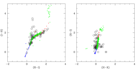
Figure 1: $R-I$:$I-H$ (left panel) and $H-K$:$R-I$ (right panel) colour-colour diagram for stars on our WHT deep field (open circles) compared with the standard star photometry of Hawarden et al. (2001), Leggett & Hawkwins (1988) and Dahn et al. (2002) (crosses).

Figure 2: $H$-band (left panel) and $K$-band (right panel) comparison between our magnitudes and those for 2MASS sources on the WHT deep field. The one galaxy is marked with an open circle. The other objects are all stellar.

4 Calibration

Calibration of the Calar Alto data was based on standard star observations made on 4 of the 5 nights. Magnitudes were measured in small apertures and extrapolated to ’total’. Standards were taken from the UKIRT faint standards list, supplemented by the data of Hunt et al. (1998). Each star was observed once in each quadrant, but all measurements from the rogue quadrant were ignored. Despite the occasional presence of cirrus, there was little difference between the four nights on which standards were taken. To monitor relative conditions (and the effect of airmass) we tracked stellar magnitudes off all the data frames throughout each night. Agreement was good, even on the nights with cirrus, with all the individual exposures finally used showing zero-points within $0.1$ mag of each other. For stars of good signal-to-noise, the rms magnitude over all frames on all nights was only $0.04$ mag. The zero-points of the final stacked frames are corrected for these variations.

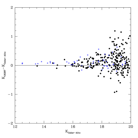
Figure 3: A comparison of galaxy magnitudes from our UKIRT data (Paper IV) and this work. There is a slight offset in that the sense that the UKIRT data are $\sim 0.06$ mag fainter. We have ignored any colour term between $K^{\prime}_{\mathrm{CA}}$ and $K_{\mathrm{UKIRT}}$.

The rms scatter about the mean offset between instrumental and standard magnitudes was $\pm 0.04$ mag in $H$ and $\pm 0.03$ mag in $K$-prime, similar to that between the data frames. We have neglected any colour term between $K$-prime and $K$. Fig 1 shows the $R-I$:$I-H$ and $H-K$:$R-I$ diagrams for stars on our WHDF $H$-band and $K$-band frames compared with stellar photometry from Leggett & Hawkwins (1988), for late-type stars, and from the UKIRT Fundamental Standards List (Hawarden et al., 2001) for earlier spectral types, and Dahn et al. (2002) from cool dwarfs. Agreement is reasonable in both cases.

We have also been able to compare our brighter stellar magnitudes with the available data from the 2MASS point source catalogue (Fig 2). Ignoring the brightest star, which is saturated, we find excellent agreement; for $H$, $H_{\mathrm{2MASS}}-H_{\mathrm{this\ work}}=-0.00\pm 0.09$ and for the $K$-band, $K_{\mathrm{2MASS}}-K_{\mathrm{this\ work}}=-0.01\pm 0.05$. Note that the faintest three stars all have 2MASS errors between 0.1 and 0.25 mags.

5 Image analysis

Our image analysis techniques have been well documented elsewhere (Papers II,III,IV, & V). In brief, the background sky is removed using a 2D polynomial fit. A first pass is then made over the data using an isophotal object detection routine to a magnitude limit much fainter than that of a $3\sigma$ detection. Objects so detected are then removed from the frame and replaced by a local sky value (plus appropriate noise). The resulting image is heavily smoothed and subtracted from the original. The isophotal object detection is then repeated on this flat-background frame. These detections are then input to a Kron-type aperture magnitude routine from which our final magnitudes are derived. Importantly, our Kron-radii are not allowed to become smaller than that for an unresolved image. Kron magnitudes require a correction to ‘total’, which ideally is independent of profile shape, but is dependent on the multiplying factor used to calculate the Kron radius. As in our previous work, we adopt an unusually small factor which results in a significant correction to ‘total’, of $\sim 0.3$ mag, but does reduce the contaminating effect of close neighbours. Even so, it is necessary to ‘clean’ such objects. Table 1 lists the parameters of all our final data frames.

Our WHDF optical-infrared and $H-K$ colours are measured in fixed $1.5^{\prime\prime}$ radius apertures. Astrometry was provided by matching to the USNO catalogue, using the STARLINK GAIA package.

We are in the fortunate position of being able to compare our Calar-Alto $K^{\prime}$-band magnitude with those from our independent UKIRT observations (Paper VI), which cover the same area and are very similar in terms of signal-to-noise. Fig. 3 shows a plot of magnitudes for stars and galaxies in common to both frames. The agreement is reasonably good right down to the limit of the photometry. For $K<16$ we find $\Delta K_{\mathrm{CA-UKIRT}}=-0.06\pm 0.06$. At $K\sim 18.5$, the noise has increased to $\sim\pm 0.3$mag.

In order to improve the signal-to-noise, image analysis was run on the stacked $K$-band frames from UKIRT and Calar Alto. The UKIRT data is slightly deeper, but the Calar Alto data has better image quality, so both images were given equal weight in the stack. Unless otherwise stated, in the rest of the paper $K$ magnitudes and $H-K$ colours refer to those from this combined data-set.

The HDF NICMOS data was analysed in similar fashion to the Calar Alto data, except that the higher resolution meant that it was often necessary to recombine images which had been artificially split by the software into several parts. Such images were identified by visual inspection of the data. A similar problem affected the HDF optical data (see Paper V), although the problem is not as severe in the NICMOS frames, due in part to the worse image quality and also due to the more regular morphology of galaxies at longer wavelengths.

5.1 Star/galaxy separation

The star-galaxy separation used on the ground-based data is that described for the WHDF in Paper V. Basically this was done on the WHDF $B$ image using the difference between the total magnitude and that inside a $1^{\prime\prime}$ aperture, a technique described in detail in Paper II. This enabled us to separate to $B\sim 24$ mag. Some additional very red stars were identified from the $R$ and $I$ frames. In $H$ this means that most objects have reliable types to $H\sim 19.5$, slightly fainter than the limit for identifications based on the frame $H$ alone, which is $\sim 19$ mag. It is possible to use $H-K$ colour as a star/galaxy separator at even fainter magnitudes – see Fig 15 (except for the bluest optical colours where late type low redshift galaxies have the same colours are main sequence stars). However, our relatively bright $K$-band limit restricts the usefulness of this in our case.

6 Galaxy Evolution Models

Before discussing our results in detail, we take a more considered look at the galaxy evolution models we have used in our previous papers. Once again we use PLE (pure luminosity evolution) models as comparison to our observed data to demonstrate that even simple models, with no assumed dynamical evolution, can well explain the observed counts (see Paper V, Metcalfe et al., 2001) and redshift distributions (Paper IV, McCracken et al., 1999).

To keep the models simple we use only two basic forms of evolution, one for early type galaxies (E, S0, and Sab) with a characteristic time-scale of $\tau=2.5$ Gyr and one for late types (Sbc, Scd, and Sdm) with $\tau=9$ Gyr, both in the context of the Bruzual & Charlot (2000) evolutionary library. We generally use a cosmology with Hubble constant of $H_{0}=50$ km s^-1 Mpc^-1 and a high ($q_{0}=0.5$) or low ($q_{0}=0.05$) density, or with a flat cosmology and cosmological constant ($\Omega_{M}=0.3$, $\Omega_{\lambda}=0.7$). The formation redshifts for these models are $z_{\mathrm{f}}=9.9$, $z_{\mathrm{f}}=6.3$, and $z_{\mathrm{f}}=7.9$, respectively. The actual cosmology used will be referred to as appropriate.

6.1 Luminosity functions

These models, when taking into account the cosmology and the attenuation due to intervening hydrogen clouds, directly predict the evolution in colour space. Convolution of this galaxy evolution (taking $e$ and $k$ corrections together) with a type dependent luminosity function (LF) finally gives us predictions for number counts, redshift distributions, colour histograms, and various other observables. This means that the LF is a critical ingredient of our modelling technique which needs to be checked, taking into account the most recent developments in the study of LFs from different surveys.

Table 2: Rest frame parameters of the luminosity function used for the PLE models ($H_{0}=50$ kms^-1Mpc^-1).

Type	$\phi^{*}$ (Mpc-3)	$\alpha$	$M_{H}^{*}$	$M_{K}^{*}$	$R$-$H$	$R$-$K$
E/S0	$9.27\times 10^{-4}$	-0.7	-24.85	-24.92	2.41	2.48
Sab	$4.63\times 10^{-4}$	-0.7	-24.27	-24.78	2.01	2.52
Sbc	$6.20\times 10^{-4}$	-1.1	-24.41	-24.83	2.03	2.45
Scd	$2.73\times 10^{-4}$	-1.5	-24.28	-24.34	2.07	2.13
Sdm	$1.36\times 10^{-4}$	-1.5	-23.70	-23.71	1.57	1.58

Figure 4: $H$-band luminosity functions. The bold solid line is our LF from Table 2, the long and short dashed lines are the LFs derived in the optical by the 2dFGRS project, and dotted and dashed dotted lines are the LFs derived in the NIR from 2MASS photometry.

The parameters of our LF (see Table 2) are derived from the ones we previously used in the optical regime (see Table 13 of Paper V). We adapted them to the NIR through the mean colours of galaxies of each type, as given in Table 2. For Paper V we checked our LF with early results of the total LF from the 2dF Galaxy Redshift Survey and found good agreement. Now we can also check our type dependent LF with that of the 2dFGRS project (Madgwick et al., 2002) in the blue $b_{J}$ band. As we are interested mainly in the performance of the LFs in the NIR regime, we convert them to the $H$-band using the mean galaxy colours for each of our 5 galaxy types. For the total LFs we density-weight the optical and NIR luminosities to form a total LF of all galaxies. The result is shown in Fig. 4. It is apparent that the LFs derived by the 2dFGRS team (Madgwick et al., 2002; Norberg et al., 2002) agree with ours to magnitudes at least as faint as $M_{H}^{\star}-6$. As the relevant SDSS publications find a good agreement between their LF and those derived by the 2dFGRS team, we skip the comparison with their data.

We also compare our LF to that derived from 2MASS data, especially the analyses by Cole et al. (2001) and Kochanek et al. (2001) that are widely used in the literature. Even when looking at the parameters of these LFs it seems that they are at odds with the ones derived in the optical: faint end slopes of $\alpha_{\mathrm{NIR}}\approx-0.9$ do not agree with $\alpha_{\mathrm{opt}}\approx-1.2$ as derived in the optical. When converting to the NIR via mean galaxy colours, the faint end slope of the 2dFGRS LFs is much steeper. This becomes clear when looking at the plot in Fig. 4 where the faint end of the NIR derived LFs has an order of magnitude less galaxies than the optically derived luminosity functions. Additionally, the NIR LFs also show a lower total galaxy density. A possible explanation for this discrepancy is already given by Cole et al. (2001): the 2MASS catalogue could be biased against faint galaxies. It is known that 2MASS misses low-surface brightness galaxies that are within the nominal magnitude limit of the survey (see e.g. Bell et al., 2003).

As in this paper we are interested in more accurate descriptions of faint galaxies and in studying galaxy properties over the whole optical to NIR wavelength range, we prefer to use the luminosity function as presented in Table 2 for our models over newer, NIR derived LFs.

6.2 Initial Mass Function

Figure 5: Observed and modelled redshift distributions presented as differential (left) and fractional cumulative redshift distributions (right) for the magnitude range $K<20$ mag. Shown are the 480 galaxies of the K20 survey of which 417 have spectroscopic redshifts (bold solid histogram). Models are: PPLE models of the K20 survey team with Salpeter and Scalo IMF (thin and bold dashed, resp.), Scalo and $x=3$ cut IMF with our LF (long-short dashed and solid lines), and a model using the Cole LF and a Salpeter IMF (short dashed).

Figure 6: Same as Fig. 5 but just for the magnitude range $18<K<19$ mag. The PPLE models of the K20 team are not available for this magnitude range, instead we show our model with Salpeter IMF.

In the past, our model predictions could only be reconciled with both the observed NIR galaxy redshift distributions $N(z)$ and the observed galaxy number counts using a non-standard initial mass function (IMF) for early type galaxies with a slope of $x=3$ and a low-mass cutoff at 0.5 M_⊙ while late types are modelled with a Salpeter (1955) IMF. Using only standard Salpeter (x=1.35) or Scalo (1986) (x=2.5 at high stellar masses) IMFs for all galaxy types would predict more high redshift galaxies than are observed (Paper IV). While some local analyses of early type galaxies do not find evidence for a steep IMF, the detailed investigation by Vazdekis et al. (1997) of several elliptical and lenticular galaxies using both broad-band colours and spectral indices confirms that a steep IMF is a possibility in at least a fraction of early-type galaxies at $z=0$.

Apart from surveys that determine the redshift distributions through photometric methods complete to some limit, the only recent spectroscopic, infra-red redshift survey is the the K20 survey (Cimatti et al., 2002a). They determined the redshifts of 480 galaxies down to a limit of $K_{s}=20$ in an area of 52 $\sq\arcmin$ to high completeness. Here, we use their redshift distribution as a test for our models. While the rest of this paper is mainly based on the $H$-band data, we have to use the $K$-band for this particular task.

First, we compare our PLE models with Salpeter (1955) and $x=3$ cut IMFs to the data and the “PPLE” models presented by the K20 team in Cimatti et al. (2002b). In Fig. 5 we show the observed redshift distribution of Cimatti et al. (2002b) together with the predictions of models with different IMFs in the magnitude range to the survey limit of $K<20$ mag. To ease comparison with the Cimatti paper, we use the “concordance” cosmology with $H_{0}=70$ km s^-1 Mpc^-1, $\Omega_{M}=0.3$, and $\Omega_{\Lambda}=0.7$ here. We also correct the models for the effect that the apparent magnitude of the bulk of the K20 sample is slightly underestimated, by computing the $N(z)$ to depths of 19.75 mag for early and 19.9 mag for late type galaxies instead of the nominal 20 mag.

The comparison in Fig. 5 presents the $N(z)$ distributions in two different ways. On the left we show the histogram of K20 spectroscopic redshifts (supplemented by a few photometric redshifts to be complete to $K=20$). As can be seen, the PPLE Scalo model that was selected as best fit model by Cimatti et al. well represents the observed distribution while their PPLE Salpeter model does not give a good fit and especially overpredicts galaxy numbers at redshifts $z>1.2$. We try to get a good match to the data with three different models: two models both using our luminosity function, one with Scalo IMF (like the one used in Paper IV) and one with the $x=3$ cut IMF, and additionally a model with Salpeter IMF and the Cole et al. LF. Of these three models, the Scalo and Salpeter models again overpredict the galaxy numbers at high redshift while the $x=3$ cut model overpredicts the numbers around $z=0.4$. On the righthand side of Fig. 5 we show an easier way to judge the quality of the fit in the form of fractional cumulative redshift distributions that show the number of galaxies with redshifts higher than a given redshift. While in this representation most models lie to the right of the data histogram, i.e. predict higher numbers of galaxies at higher redshift, the $x=3$ cut model very well fits the overall shape of the data if local variations due to clustering are disregarded. The fit for this model is even better than for Cimatti et al.’s Scalo model, especially at high redshifts with $z\gtrsim 0.8$.

While the comparison of the $N(z)$ shape is difficult with samples of this relatively small size because of the effect of clustering, which dominates the histogram in certain redshift slices, one can also use the median redshift as a quick measure of how well the models compare to the data. The median survey redshift is given as $z=0.74$ for all 480 galaxies (or $z=0.81$ disregarding the clusters at $z\sim 0.7$). This as well as the median redshifts of the different models can be read off the graph in Fig. 5b. The PPLE Scalo model ($z_{\mathrm{med}}=0.78$) and the $x=3$ cut model ($z_{\mathrm{med}}=0.75$) very well agree with the median redshift of the survey while the models with all other IMFs (PPLE Salpeter, $z_{\mathrm{med}}=0.98$, our Scalo model, $z_{\mathrm{med}}=0.90$, and our Salpeter model with Cole LF, $z_{\mathrm{med}}=0.95$) do not match the observed data.

In Paper IV we chose to use the model with $x=3$ cut IMF as our main model after comparing redshift distributions in the magnitude range $18<K<19$ mag. We therefore carry out an additional test with a subset of the K20 data in this magnitude bin. The result is presented in Fig. 6. While it is not possible to test how well the models of the K20 team compare to these data, we can conclude that, amongst our models, that with the $x=3$ cut IMF has the best fit. Again, it does not seem to be possible to get a similarly good agreement using other IMFs like Scalo or Salpeter, even if the Cole luminosity function is used.

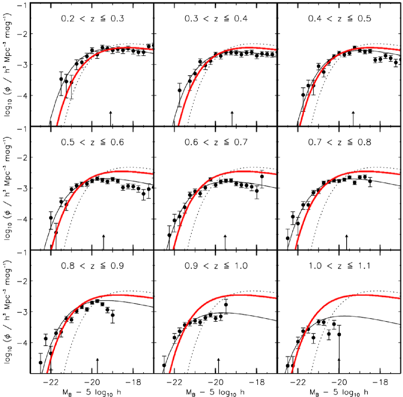
Figure 7: Comparison between our predicted LF’s for E/SO galaxies (bold solid line) with those from the COMBO-17 photometric redshifts of Bell et al. (2004) in the rest $B$-band. The light solid line represents the fit of Bell et al. (2004) to the observed LF and the dashed line represents the SDSS local E/SO LF.

Finally, we compare our predictions for E/SO galaxies out to $z\approx 1$ with the photo-z COMBO-17 data of Bell et al. (2004, see Fig. 7). The COMBO-17 LFs are expressed in the rest $B$-band. The models again appear to give a reasonable fit to the data out to $z\sim 0.8$ which shows that the small amount of luminosity evolution in the data is well matched by the $x=3$ model. In addition, we also find our early-type model is in good agreement with preliminary results from 2dF-SDSS redshift survey of Luminous Red Galaxies out to $z\approx 0.7$ (D. Wake, priv. comm.). Early results at even higher redshift from the VIMOS/VLT Deep Survey also show virtually no evolution for the red galaxy LF and strong luminosity evolution for the blue galaxy LF (Le Fevre et al., 2004), both characteristics of our PLE models.

These results show that even the simple models with just two basic types can be used to quite well interpret data in deep fields and redshift surveys and that the models with the $x=3$ cut IMF, only slightly steeper than the Scalo IMF at high stellar masses, agree best with the data available to us. We, therefore, again adopt this model, with the $x=3$ cut IMF and luminosity function as in Table 2, as our main model.

7 Results & Discussion

7.1 $H$-band counts

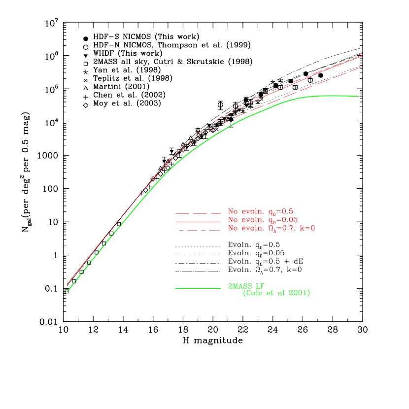
Figure 8: $H$-band number-counts from the literature and from our current work. A correction has been applied to the number counts of Thompson et al. (1999) using their supplied incompleteness corrections. Also shown are the predictions of the various models discussed in the text – a low- and high- $q_{0}$ non-evolving model, together with a non-evolving lambda model, and four evolutionary models, low and high $q_{0}$, high $q_{0}$ with an added dwarf galaxy component and a spatially flat lambda model. All of these assume the LF parameters in Table 2. The 2dFGRS/2MASS model is based on the LF of Cole et al. (2001) and assumes the same PLE $k+e$ corrections as the other evolutionary models for the red and blue galaxies.

In Fig. 8 we show our differential $H$-band galaxy number-counts measured in the WHDF and from the HDFS NICMOS frame, as well as counts from the literature. Poisson error bars are shown where available. There is now very good agreement between the published datasets in the range $16<H<21$. Faintward of this the scatter increases, but it must be remembered that these data come from very small areas of sky, and that cosmic variance has not been included in the error bars. The counts at bright magnitudes are the 2MASS all-sky XSC counts above a galactic latitude of $\pm 25\deg$, with a $0.15$ mag correction (Jarrett et al., 2000) to total magnitudes and show that the normalisation of the models (which adopt the $B$-band luminosity function extrapolated to $H$ using the rest-frame colours of galaxies) is reasonable (see Frith et al. 2003 for a discussion of a local underdensity in the infra-red counts).

Table 3 lists the $H$ counts from our Calar Alto data. Table 4 details the HDFS NICMOS counts. To transform from $F160W_{AB}$ to $H$ requires a brightening of 1.3 mag (as computed with the synphot tool).

To allow for the extended nature of many galaxies, we only quote our counts to $H=22.5$ rather than the $3\sigma$ limit for stellar sources of $22.9$ mag.

Table 3: $H$-band differential galaxy counts from the 14hr Calar Alto frame.

Magnitude	Raw Ngal
($H$)	(frame total)	($\deg^{-2}$ (0.5mag)-1)
17.0-17.5	18	1349
17.5-18.0	16	1199
18.0-18.5	24	1798
18.5-19.0	32	2398
19.0-19.5	49	3672
19.5-20.0	105	7868
20.0-20.5	109	8167
20.5-21.0	169	12663
21.0-21.5	226	16934
21.5-22.0	314	23528
22.0-22.5	419	31396

Table 4: $F160W_{AB}$-band differential galaxy counts from the HDF South NICMOS field.

Magnitude	N${}_{gal}\hfil$
($F160W_{AB}$)	(frame total)	($\deg^{-2}$ (0.5mag)-1)
23.0-24.0	18	35900
24.0-25.0	32	64000
25.0-26.0	63	125500
26.0-27.0	78	155500
27.0-28.0	138	275500
28.0-29.0	126	251500

At brighter magnitudes our work agrees with the published counts. In particular, our counts are close to those from the $0.4\,\sq^{\circ}$ area published by Chen et al. (2002). Faintward of $H\sim 22.5$ (where all the counts are HST based) we find our HDFS counts higher than the HDFN counts of Thompson et al. (1999), but lower than Yan et al. (1998). This may be due to cosmic variance, or even differences in the way that the various data reduction software cope with the tendency of faint objects to break into sub-detections (section 5).

In the main, we consider model counts based on the LF parameters in Table 2, for consistency with the work in the optical count models in Paper 5. As noted in Sect 6.1 there is reasonable agreement between this and other more recently determined optical LFs at brighter absolute magnitudes, although infra-red determined LFs seem to have a flatter faint end slope. We shall see that this variation in slope will cause differences in interpretation of the faintest HDF counts.

As far as comparison with the PLE models with the LF parameters in Table 2 is concerned, it is apparent that faintwards of $H\sim 21$, our number counts are higher than the predictions of the both the evolving and non-evolving $q_{0}=0.5$ models; the faint end of the $K$-selected counts has already hinted at a similar trend, as illustrated in Fig. 1 in Paper IV. Apart from this you would be hard pressed to distinguish between the various models. The alternative dwarf-dominated $q_{0}=0.5$ model proposed by Metcalfe et al. (1996) to explain the optical counts is probably too high to fit the faintest bins of the HDF data, but could be lowered at faint magnitudes somewhat without destroying the agreement in the optical (Paper V) (In this “disappearing dwarf” model, the dwarf population has constant star-formation rate at $z>1$ and fades rapidly at $z<1$). The $\Lambda$ dominated cosmology gives too high a count at intermediate magnitudes ($19<H<21$) for our relatively high normalisation (see Paper V for a discussion of the choice of normalisation), but would probably satisfy those who favour a lower value. Our $q_{0}=0.05$ $x=3$ evolutionary PLE model reproduces the observed number counts well.

Of course, if has been known for some time that the optically selected number counts diverge from the $q_{0}=0.5$ NE model, at around $B\sim 20$, when the effects of evolutionary brightening become significant. And at NIR wavelengths we expect the morphological mix to become spiral dominated faintwards of $K\sim 20$, so it is not too surprising that the counts should be above the predictions of the non-evolving $q_{0}=0.5$ model, which, after all, fails to reproduce the number counts correctly in all other bandpasses. The amount of passive evolution in $H$ must still be small by $H\sim 22$, however, given that our observations are close to our $q_{0}=0.05$ evolutionary model, which has been specially tuned to reduce the amount of passive evolution. Furthermore, the angular correlation function of this sample, discussed in McCracken et al. (2000), appears also to favour an essentially non-evolving redshift distribution at these depths.

Finally, Fig. 8 also shows results from modelling the galaxy number counts with the more recent NIR LF of Cole et al. (2001). In the context of our simple models using two basic evolutionary tracks, these LFs produce less good fits to the faint H counts. Whether we use just the total LF (as given by Cole et al., 2001, converted to the $H$-band) with $M_{H}^{*}=-24.73$ and $\alpha=-0.96$ and assuming an early-type $k+e$ correction, or use the LF split between our two evolutionary galaxy types, it is not possible to derive a good fit to the data, irrespective of other model parameters like IMF or characteristic time-scale $\tau$; the counts are too flat at the faintest magnitudes (see Fig. 8.) Even if the $\approx 1.8\times$ higher normalisation, as assumed by our models, is used, the predicted count would still be too low to fit the data via a PLE model. We should also emphasize the importance of the normalisation in determining how well models fit. Our normalisation is taken at $B\approx 18.5$ to avoid the issues with large scale structure at brighter magnitudes (see Busswell et al., 2004; Frith et al., 2005).

Thus if the local galaxy LF is closer to that given by our parameters in Table 2, then the good fit of the models to the faint counts suggest that the galaxy LF at high redshift($z\approx 1$) has a slope similar to the present day, with no need to evoke evolutionary steepening. This means that there is no immediate detection of the steep LF at $z\ga 1$ that would better match the generically steep halo mass function of CDM models. However, if the flatter local LF of Cole et al. (2001) is taken then evolutionary steepening of the LF may be necessary at high redshift. The main argument against the Cole et al. (2001) 2MASS LF is that it does not seem consistent with the steeper LFs found when optical LFs are converted to the H band using straightforward colour transformations of the galaxy sub-populations. More checks of the 2MASS H band magnitude scale as used by Cole et al. (2001) are required. If the 2MASS magnitudes are correct then the excellent fit of our almost unevolving PLE models to the data in the range $10<H<28$ may then have to be taken as coincidental.

In summary, if the infra-red galaxy LF we have derived from the optical LF is accurate then there is no need to invoke any evolution in the form of the galaxy LF in the range $0\la z\la 2$ to fit the $H$-band counts. The excellent fit of almost a non-evolving model throughout the range $H<28$ mag range then may be an excellent indication that the high and low redshift Universe may be more similar than usually expected. However, if the local LF has a flatter slope and/or a lower normalisation then this slowly evolving model is less consistent with the faintest $H$ counts data.

7.2 Colours

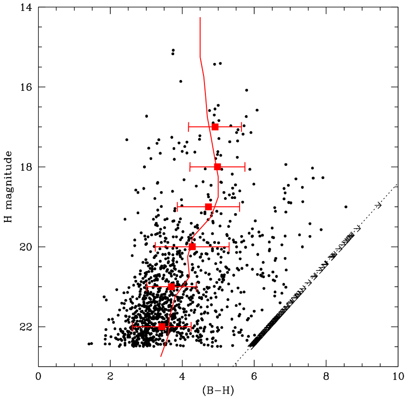
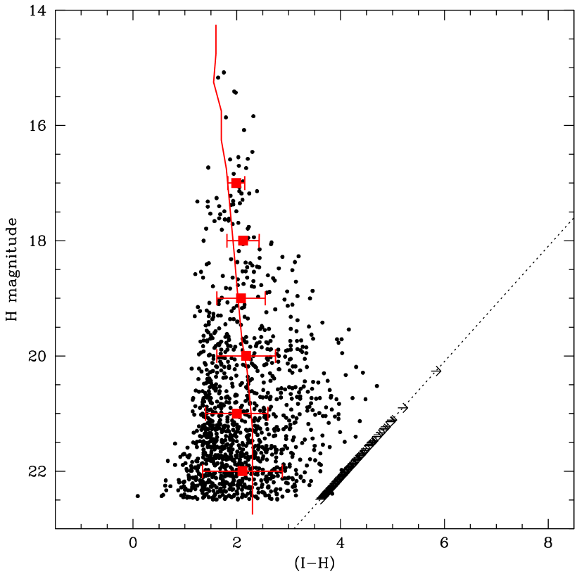
Figure 9: $H$ magnitude against $B-H$ colour for galaxies in the WHDF, with median colours calculated in one magnitude bins. The median of our evolving $q_{0}=0.05$ $x=3$ model is also shown (solid line). The dashed line shows the region of incompleteness. Right-pointing arrows show objects too red to be detected in the optical band.

Figure 10: As in Fig. 10, but instead $H$ magnitude against $I-H$ colour is plotted.

Fig. 10 and Fig. 10 show optical - infra-red colours for $H$-selected objects in the WHDF. If compared to fig. 2 of Paper IV it is apparent from these graphs that the Calar Alto dataset is a considerable advance over our old UKIRT wide survey, which was limited at $K\sim 20$. This work effectively extends our $3\sigma$ limit two magnitudes fainter with the same area coverage and with reduced photometric errors. In Fig. 10 we plot $B-H$ colour against $H$ magnitude for all objects to $H<22.5$; also shown are median colours (filled squares), and the predictions for the median colours of the $q_{0}=0.05$ $x=3$ evolutionary model. Fig. 10 is identical to Fig. 10 except that in this case we plot $I-H$ as a function of $H$ magnitude. This can be compared directly with fig. 9 of Chen et al. (2002).

In Fig. 10 the median $B-H$ colour becomes slightly redder to $H\sim 18$, after which it turns bluewards and this trend continues to the the limit of our survey. This should be compared to our previous $K$ vs $B-K$ plot (fig. 2 of Paper IV), which shows a similar trend for the non-evolving models. There, however, a large apparent gap was seen in the data near $K=21$, $B-K=5.8$ where very few galaxies were detected although this was above the detection threshold in both filters. In the present data this gap is not quite as obvious, although there is still a blueward turn of the median of the median colour faintwards of $H\approx 20$.

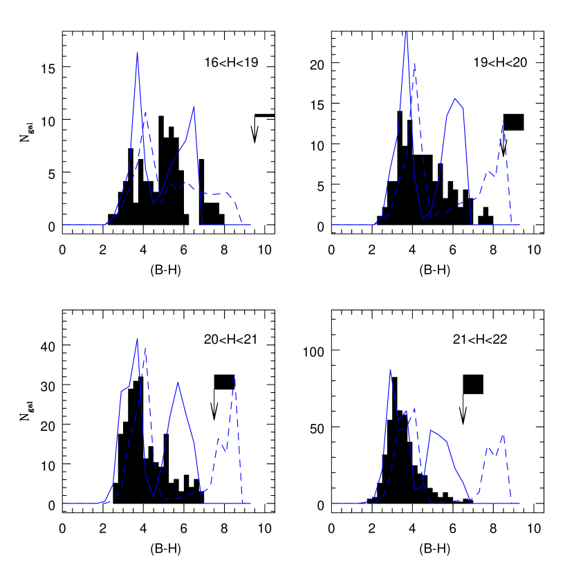
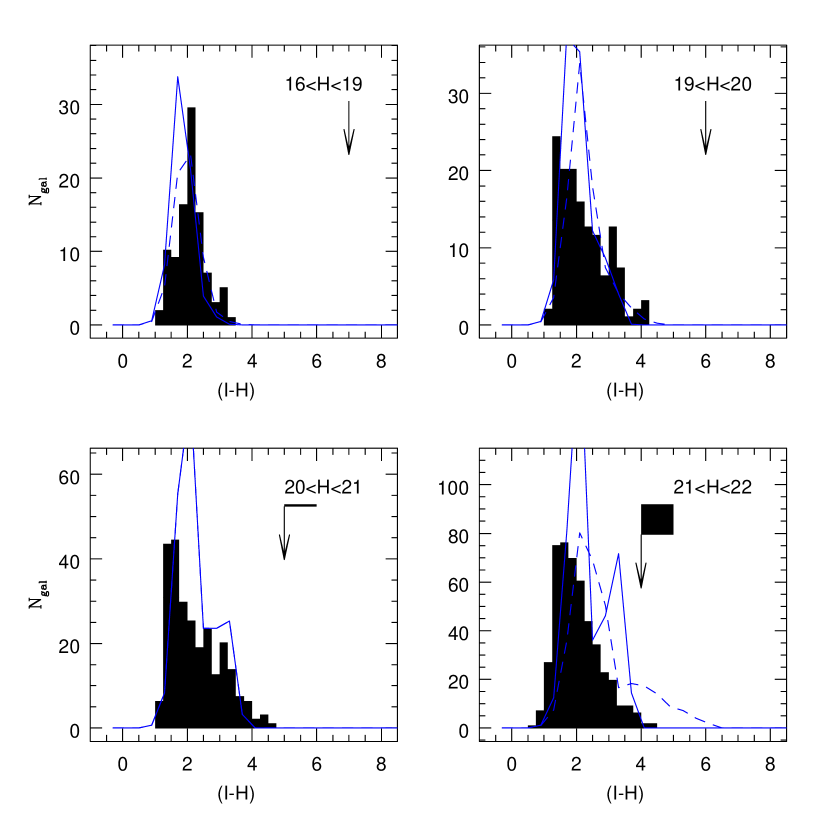
Figure 11: $H$ selected $B-H$ distributions; arrows show the colour completeness limit – the area of attached box shows the number of objects with no measured colour. The solid line show the predictions of the $q_{0}=0.05$ $x=3$ evolutionary model. The dashed line is the non-evolving counterpart.

Figure 12: $H$ selected $I-H$ distributions for the Calar Alto dataset. All symbols are identical to Fig. 12.

The histograms of galaxy colours show this bluewards movement more clearly. In Fig. 12 and Fig. 12 we present the $B-H$ and $I-H$ colour distributions for objects in the WHDF selected by $H$ magnitude in four slices from $16<H<19$ to $21<H<22$. The dashed lines show the predictions of a non-evolving model, whereas the solid lines show the predictions from the $x=3$ evolutionary model. We have not renormalised the models counts to agree with the data in each bin, and as a result the evolutionary histogram slightly overpredicts the numbers of objects.

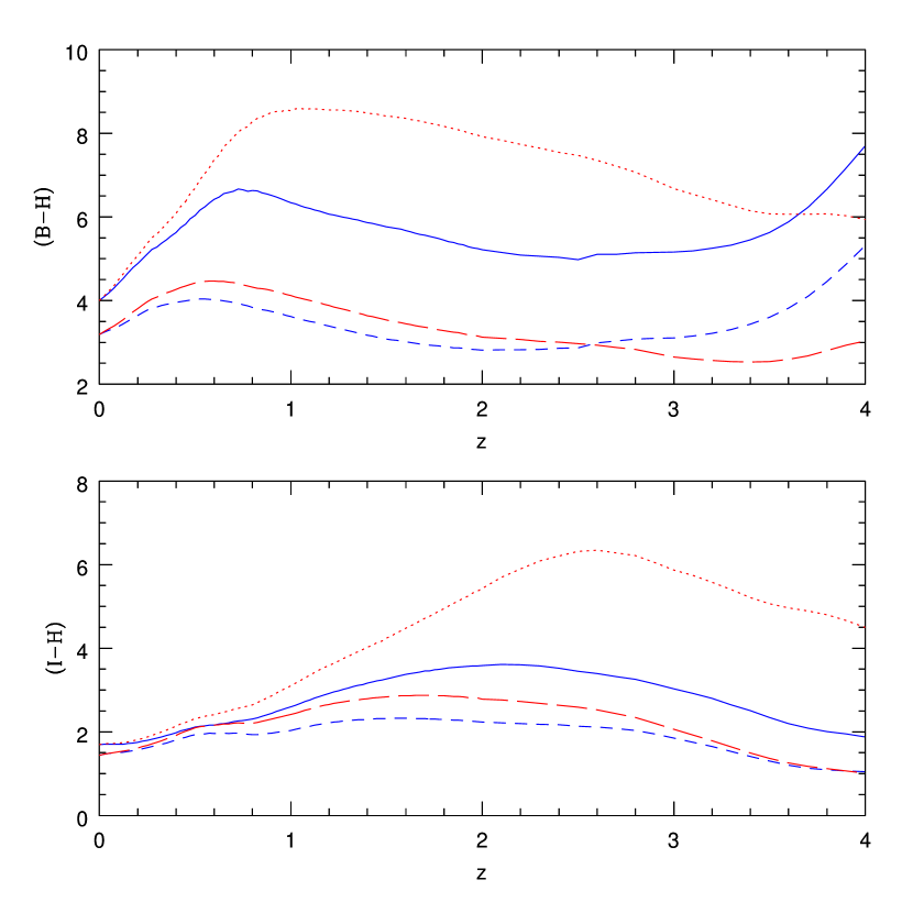
Figure 13: $I-H$ colour (lower panel) and $B-H$ colour (upper panel) as a function of redshift for our $q_{0}=0.05$ model; non evolving E/S0 (dotted line), evolving E/S0 (solid line), non-evolving spiral (short-dash), evolving spiral (long-dash).

These diagrams confirm the broad conclusions presented in Paper IV; we find that the numbers of extremely red, unevolved objects present in these distributions are extremely small. In Fig. 13 we plot $I-H$ and $B-H$ colour of our models as a function of redshift. A non-evolving galaxy track (i.e., a pure $k$-correction) reaches $I-H\sim 6$ by $z\sim 2$, or $B-H\sim 8$ by $z\sim 1$. Our survey shows a conspicuous lack of such objects. However, even with our $x=3$ model there is a red peak predicted in the colour distributions at $B-H\sim 6$ and, in the faintest bin, at $I-H\sim 3$ which is not seen in the data. These are the evolved E/S0s at $z>1$, which although much bluer than non-evolving predictions, still should be present in our sample.

Following, Paper IV, it is worth considering the $I-H$ histograms in Fig. 12 more carefully. While the brighter H bins continue to show the slightly extended red tail that indicates the continuing presence of the early-type galaxies, by the faintest $21<H<22$ bin, there may be more of a case that these galaxies could have disappeared (de-merged). However, these galaxies may have simply moved bluewards faster than the PLE model as the UV flux enters the I band at $z\approx 1$, as appears to have happened already in the B band (see Fig. 12) for galaxies 2mag brighter in H. Indeed, renormalising the model prediction downwards suggests that the overall shape of predicted $I-H$ distribution may still fit the data even in this faintest bin. Thus we conclude that the early-type galaxy population may persist essentially unchanged except in the UV out to $z>1$, as indicated by the continuing excellent fit of the PLE models in $I-H$ to $H\approx 22$ mag.

Fig. 15 shows $B-R$ vs $R-H$ for all galaxies in the WHDF, as well as the colour tracks predicted by the models. In this plot, galaxies have been split by magnitude, with the filled circles representing galaxies with $H<19$. From this it is apparent that a large number of the faintest galaxies lie in the region of this plot occupied by spiral galaxies. This is not unexpected, as indicated by Fig. 16, which shows the number counts from our model for the individual morphological types.

As noted in Paper IV, and by Chen et al. (2002), there is a large scatter in the colour-colour plane, with galaxies distributed over a very broad range of optical - infra-red colours, particularly for the objects the models tracks suggest should be early types (remember that for clarity we only show one spiral track, but in reality the Sbc-Irr tracks will represent most of the bluer colours). The large scatter could explain the flat distribution in Figs 12 and 12 compared to the models at $B-H\sim 6$ and $I-H\sim 3$. This is discussed further in the next section, but may be evidence of a wide range of star formation histories, dust content, or metallicities for the early types. It is interesting to speculate whether the intermediate population of ‘blue’ early-types detected by Vallbe et al. (in prep.) at $z<0.5$ are now contributing at higher redshifts to the wide scatter in $R-H$ at $z>0.5$. The problem is that the scatter is as much on the red side of the track as on the blue in this redshift range. However, the early-type track in $R-H$ is quite sensitive to e-folding time of the SFR, $\tau$ (which is degenerate with the IMF slope). It may be possible to choose $\tau<2.5$Gyr in the $x=3$ case to make the track more like a red envelope in the $B-R:R-H$ diagram at $0.5<z<1.5$ while not making the track too red at $z\sim 0.5$ in $B-R:R-I$. Then the scatter would shift to the bluewards side and be explained by on going star-formation in the intermediate early-type population.

Fig. 15 shows $H-K$ vs $R-I$. This time we curtail the distribution at $H=20$, due to the bright limit of the $K$ data. This confirms the suggestion from the optical data in Paper V that the galaxies redder than $R-I\sim 1$ are likely to be early types in the range $0.5<z<2$.

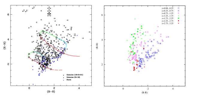
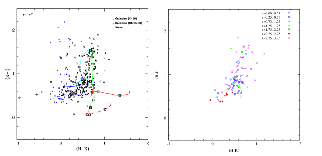
Figure 14: Left: $H-K$ vs $R-H$ plot for all galaxies and stars on the WHDF with $H<21$. Filled and open circles represent galaxies brighter and fainter than $H=19$ respectively. Colour limits for those not detected in $R$ are shown with arrows, assuming a magnitude $0.5$ mag below the $3\sigma$ $R$-band detection threshold. A double horizontal arrow indicates galaxies not detected in $B$ or $R$ (i.e. its $B-R$ colour is undetermined). Also shown are the Bruzual and Charlot tracks for E/S0 galaxies (solid line) and Scd galaxies (dashed line). Redshift intervals of $z=0,0.5,1,1.5,2,2.5,3,3.5$ are marked with boxes. Right:the same colour-colour plot, but only for those galaxies assigned photometric redshifts from Hyperz with $>80$ per cent probability. Redshift ranges are indicated by the different symbols.

Figure 15: As Fig 15 but now for $H-K$ vs $R-I$ and limited at $H=20$.

To illustrate these points further, we also carried out a comparison of photometric redshifts of the $H$-band selected galaxies with our elliptical and spiral models. The photometric redshifts were derived using the Hyperz package (Bolzonella, Miralles, & Pelló, 2000), publicly available at http://webast.ast.obs-mip.fr/hyperz/. As input to Hyperz we used our catalogue of galaxies with $H<21$ mag and a maximum of six magnitudes in the filters $U$,$B$,$R$,$I$,$H$, and $K$. We let Hyperz compute the most likely redshift in a range $0.1<z<6.0$ with steps of 0.05 and a possible internal reddening $0.0<A_{V}<2.0$ mag with the Calzetti law (Calzetti, 1997). The full set of observed and model templates coming with Hyperz was used to cover all observed types, but checks with limited template samples showed no significant difference. To be consistent with our previous results we used the cosmology with $H_{0}=50$, $q_{0}=0.05$ without a cosmological constant. The weighted mean redshifts with corresponding confidence probability better than 80 per cent were selected. A check with known redshifts in the WHDF suggests typical errors of $\delta z=\pm 0.10$ (for $z<0.5$) if the object is observed in all six filters. The result is shown in the right-hand panels of Figs. 15 and 15.

In general, we find a good agreement between the our model tracks and the photometric redshifts of our galaxy sample in these two-colour diagrams. Our model tracks in the range $0.0<z<0.5$ are close to the centre of the area covered by the objects with the photometric redshift in this range as shown in the $B-R$ vs $R-H$ colour plane (Fig. 15). Only a few $z>2.25$ objects are scattered in the region where our models have redshifts below $z=2$. Note that the location of the low redshift galaxies in this diagram is about the same as that of the brighter $H<19$ galaxies is in Fig. 7. The galaxies with bright apparent magnitudes are therefore mostly low redshift objects.

In the $H-K$ vs $R-I$ two-colour plane (Fig. 15) the photometric redshifts of only the lowest redshifts ($z\la 0.5$) agree with the corresponding model tracks of Fig. 8. The objects in the range $0.75<z<1.25$ are distributed over the whole diagram, whereas this redshift range in the model tracks is located in a very small area. And especially the $z>2$ objects are much bluer in $H-K$ than our model tracks predict. This is due to the type selection of the Hyperz templates: the best fit template of the $z>2$ objects is a starburst seen at a young age, a case not included in our simple models.

Figure 16: $H$-band number-magnitude relation as a function of morphological type for the evolutionary $q_{0}=0.05$ model. The heavy solid line shows the total predicted galaxy count.

7.3 EROs

Table 5: Numbers of EROs with $R-K>5$, $K<19.2$ per $\sq\arcmin$ and as a percentage of all galaxies with $K<19.2$.

Author	$N_{\mathrm{ERO}}/\sq\arcmin$	Percentage
Model ($x=3$)	0.67	11
Model (Salpeter)	2.7	29
This work	$0.53\pm 0.1$	$15\pm 0.03$
Daddi et al. (2000)	0.63	13
Cimatti et al. (2002a)	0.88	$13\pm 0.02$
Roche et al. (2003)†	0.5	13

^† Estimated from values at $K=19$ and $K=19.5$

Much attention has been devoted in recent years to the study of Extremely Red Objects, or EROs (e.g. Cimatti et al. 2002a, Smith et al. 2002, Roche et al. 2003, Yan & Thompson 2003). These are objects traditionally selected to have $R-K>5$, although as is clear from Fig. 15 and Fig. 3 of Paper IV, this has little meaning in the context of modern evolutionary models other than to select E/S0s roughly in the range $1<z<2$. Nevertheless, we show a comparison of our numbers for $R-K>5$ with other published values in Table 5. Although the absolute numbers vary, the percentage of EROs is remarkably constant between authors. We also show the prediction of the $q_{0}=0.05$ $x=3$ model, and a standard Salpeter PLE model. Several problems affect these comparisons; firstly the red extreme of the model tracks is very sensitive to the exact star formation history adopted, and, secondly, $R-K=5$ is on a steeply falling portion of the number-colour histogram, so small uncertainties in zero-point and random errors on the colours (and potentially colour equations between $K$-bands used at different observatories) could make substantial differences to the numbers. The surface densities found by Daddi et al. (2000) differ by almost a factor of two between samples with $R-K>5.0$ and $R-K>5.3$. Nevertheless, the $x=3$ model predicts both a similar percentage as the data and absolute densities close to the mean observed density at $R-K>5.0$. Our Salpeter PLE model is a factor of two higher, as expected from the results in Sect. 6.2 where it was shown that this model predicts far too many objects above $z=1$. Remaining small differences in the $x=3$ model can be explained by the observational result of Cimatti et al. (2002a) who presented evidence that a large fraction of the ERO population are dusty starburst galaxies. A similar conclusion was reached by Yan & Thompson (2003), who found from HST imaging that about 65 per cent of EROs were showed disks, although Yan et al. (2004) found that the fraction of emission line objects was similar amongst both bulge and disk domimated EROs. As dust does not have a large effect on the numbers of NIR selected galaxies it would shift the galaxy population towards redder colour, so that the inclusion of dust in our models would result in a somewhat higher number of EROs predicted. As the deviation of the modelled number of EROs from the mean observed number is smaller than the deviation between different the number from observational projects, it makes little sense to try and finetune this parameter.

This success of the $x=3$ models with our new data and other data from the literature somewhat contrasts the analysis of Smith et al. (2002). They observationally found an order of magnitude more EROs (colour cut $R-K>5.3$) than predicted by our model from Paper IV, in contrast to more specialised models of Daddi et al. (2000). Since our early-type track does not reach $R-K=5.3$ at any redshift, it is clear that our simple model will underpredict the the numbers of EROs with a very red cut.

Table 6: Numbers of objects with $I-H>3$ per $\sq\arcmin$ with $\pm 1\sigma$ errors over the $1.26\times 10^{-2}$ deg² of the deep $H$ image which has $I-H$ colours. Objects too red to have a measured colour are included.

Author	$19<H<20$	$20<H<21$	$21<H<22$
Model (evol.)∗	$0.3$ (8%)	$1.4$ (18%)	$4.1$ (27%)
Model (NE)	$0.5$ (16%)	$1.7$ (27%)	$3.4$ (29%)
This work	$0.55\pm 0.1$	$1.17\pm 0.2$	$2.1\pm 0.2$
	(18%)	(21%)	(20%)
Chen et al. (2002)	$0.42$ (15%)	$1.1$ (20%)	$-$

^∗ Evolving model with $q_{0}=0.05$ and $x=3$ IMF

Figure 17: The number-counts of EROs with $I-H>3$. Filled circles, this paper; open squares, Chen et al. (2002). Our faintest point is on the limit of the $I$-band photometry and should be treated with caution. The solid line shows the prediction of the $q_{0}=0.05$ $x=3$ model, the dashed line that of the non-evolving $q_{0}=0.05$ model.

With our deeper $H$-band data we can study the distribution in $I-H$ as previously done by Chen et al. (2002). Table 6 shows the numbers of objects with $I-H>3$ – a colour-cut that is roughly equivalent to $R-K>5$, although it selects a slightly higher redshift range – for three $H$ magnitude bins. For the bins in common, we find excellent agreement between our data and that of Chen et al.. We show the $H$-selected ERO counts subdivided into smaller $0.5$ mag bins in Fig. 17. While Chen et al. suggested that the number counts turn over at $H\sim 20$ it is clear from our deeper $H$-band data that this does not happen. Instead, the counts continue to rise towards our faintest bin centred $H=22.25$ mag.

When comparing our models to these data we find that on average the numbers are in good agreement with the observed numbers of ERO galaxies. This is true for both our no-evolution model and the evolving $x=3$ model. For $21<H<22$ the models predict 27–29 per cent $I-H>3$ objects, compared with 20 per cent seen in the data. As indicated by Fig. 11, our ERO count predictions using $B-H$ limits will be in much less good agreement with the data, although as pointed out in Paper IV, due to the sensitivity of the $B$-band to evolution, these colours can be changed quite drastically by small changes in IMF or star-formation rate e-folding time.

The location of our EROs with $H<21$ in four colour-colour planes are shown in Fig. 18, together with our early-type model track. The data show a large scatter (of over 1 magnitude), but in all the plots tend to cluster around the $z\sim 2$ model location. Nearly half our EROs are detected in the $U$ band, but this should not be taken as evidence of unusual star forming activity, as the model colour for an E/S0 at $z\sim 2$ is $U-H\sim 5.5$, well within the range of our $U$ data for $H<21$.

7.4 The Early-type Sequence

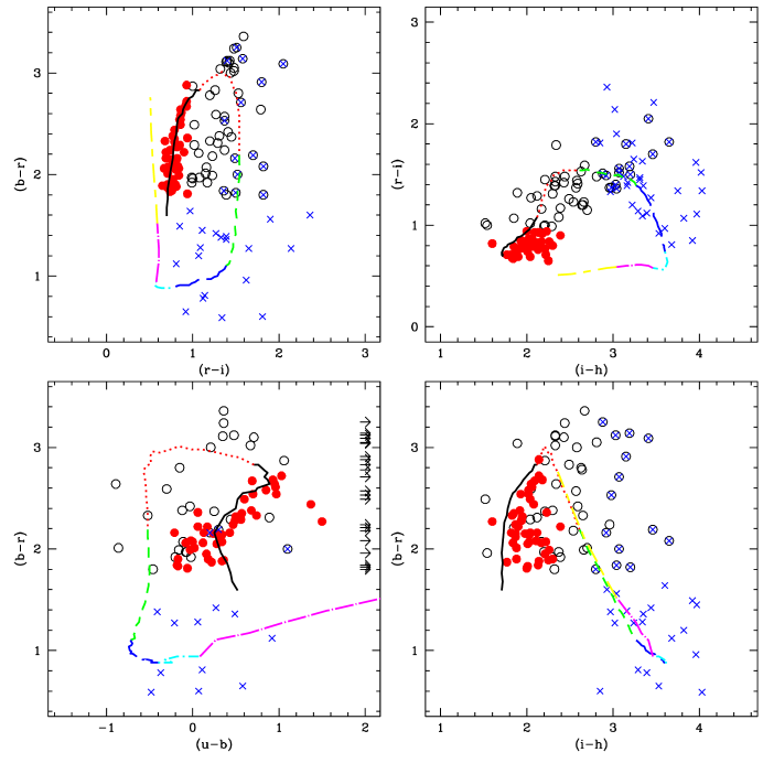
Figure 18: The colour properties of E/S0 ’sequence’ galaxies. Shown are four colour-colour diagrams (all limited at $H<21$) for galaxies selected on the basis of their location in the $R-I$:$B-R$ plane (top left). Solid circles, $B-R>1.8$, $R-I<0.95$ – these are identified as E/S0 galaxies with $z<0.5$; open circles, $B-R>1.8$, $R-I>0.95$ – potential E/S0 galaxies in the range $0.5<z<1.0$ . Also shown, as crosses are the location of EROs defined as $R-K>5$. Our $q_{0}=0.05$ $x=3$ evolving model for E/S0s is shown; solid line, $0<z<0.5$; dotted line, $0.5<z<1.0$; short dashed line, $1.0<z<1.5$; long dashed line, $1.5<z<2.0$; short dash-dot, $2.0<z<2.5$; long dash-dot, $2.5<z<3.0$; long dash short dash, $3.0<z<3.5$.

Previous studies (with the exception of Firth et al. 2002) have tended to concentrate simply on one colour. Our multi-wavelength data enables us to explore galaxies with particular properties in different two-colour planes. In particular, in Paper IV we showed how the $R-I$:$B-R$ plane seems to provide a means of selecting early-type galaxies. According to the models, the clear ’sequence’ seen with $B-R>1.8$ and $R-I<0.95$ delineates E/S0 galaxies with $z<0.5$. In fact this is insensitive to choice of model – a simple $k$-correction would come up with a similar cut. The models also suggest that $B-R>1.8$ and $R-I>0.95$ should select E/S0s between $0.5<z<1$. The $H$-band is ideal to study if this truly selects early type galaxies. In Fig. 16 we plot the contribution of the various morphological types of galaxy to the $H$-band number-counts for our $q_{0}=0.05$ $x=3$ model. It can be seen that early type galaxies are the most numerous type up to $H\sim 22$. Fig. 18 shows the location of our colour selected E/S0s with $H<21$ (this ensures good colour completeness in all except $U-B$) in four colour-colour planes, together with the redshift coded model tracks for E/S0s. The reader’s attention is drawn to the fact that many of the low $z$ galaxies at $B-R\sim 2$ appear too blue in $U-B$ and too red in $I-H$ to be normal E/S0s, suggesting that these galaxies have experienced more recent star-formation than contained in our simple PLE model. This may be evidence for an intermediate population of early-type galaxies. Furthermore, some of these galaxies, although lying on the early-type sequence in $R-I$:$B-R$, have been found to have bluer $B-R$ colours than expected for their redshift, again suggestive of an intermediate age early-type population. This is discussed by Vallbe et al in prep where evidence for an intermediate early-type population in a 2dFGRS/SDSS dataset is also investigated.

Recently, new modelling techniques that include the thermally pulsing asymptotic giant branch (TP-AGB) of some stars were suggested (see e.g. Schulz et al., 2002) that find much redder optical-NIR colours for stellar populations of ages $>10^{8}$ yr, a feature that was successfully tested on globular clusters (Maraston et al., 2001) and distant galaxies (Schulz et al., 2003). This property is not included in our models based on GISSEL99 (Bruzual & Charlot, 1993), but a combination of this feature and moderate amounts of dust may well produce a UV excess plus extra optical-NIR reddening in intermediate age stellar populations, as seen for the early-type galaxies in Fig. 18. The spectral properties of these galaxies will be discussed in a subsequent paper where we will also explore the effect of refinements of our modelling technique including the TP-AGB.

7.5 A new high-$z$ galaxy cluster

Figure 19: (a) The position of galaxies with $I-H>2.5$, $R-I>1$ over the $7^{\prime}\times 7^{\prime}$ field of view of the WHDF. The region containing a possible new high redshift galaxy cluster is highlighted. (b) Distribution of $R-H$ colours for galaxies in a 2.35 $\sq\arcmin$ region centred on our proposed cluster (solid histogram), compared with the distribution for the whole field, normalised to the same area (dashed histogram).

Our colour selection has identified a possible high redshift cluster on the WHDF. Selecting galaxies with colours $I-H>2.5$ and $R-I>1$ and plotting their location on the sky, shows a pronounced overdensity of some 20–25 galaxies of objects within a diameter of $1.5^{\prime}$ ($\sim$ 0.5$h^{-1}$ Mpc at $z\sim 1$) in a region near the NW corner ($00^{h}22^{m}45.2^{s}$, $0\degr 23^{\prime}26^{\prime\prime}$) of our $7^{\prime}\times 7^{\prime}$ field of view. This region is highlighted in Fig. 19a. A histogram of galaxy $R-H$ colours within this region in Fig. 19b (solid line) shows a second peak at $R-H\sim 4.5$ while there is no extra peak in galaxy colours over the whole field (dotted line). Using our optical and NIR magnitudes of the possible members of this cluster we have computed photometric redshifts with Hyperz and find that most of these galaxies are between $1<z<1.5$, most likely in the lower half of this redshift range. The brightest three galaxies in the region have $H\sim 19$, although the one nearest the apparent centre of the concentration has very blue colours, which would imply a lower redshift late-type galaxy.

Of course, these are only indications for the discovery of a new galaxy cluster at $z\gtrsim 1$, which would require spectroscopic follow-up for confirmation. But even so one might speculate about the apparent shape of the overdensity which does not seem to be spherical but more elongated. Although the cluster is detected near the edge of our field of view and we should be careful not to overinterpret this, we might be looking at a cluster in formation where galaxies from the surrounding filaments are falling into the gravitational potential of the cluster.

8 Conclusions

We have presented data from deep NIR observations of the William Herschel Deep Field down to $H\sim 22.5$ mag. These data reach about two magnitudes deeper than previous “wide area” observations in the NIR (see Paper IV) and now extend over the full central $7^{\prime}\times 7^{\prime}$ of the WHDF. Several conclusions can be drawn from these new data and in comparison with our models. These PLE models assume a bimodality in SF history; red galaxies essentially evolve passively after an initial burst of star-formation at high redshift whereas blue galaxies evolve with star-formation only decaying with an e-folding time of 9 Gyr.

In our investigation about input parameters for our PLE models we noticed that a discrepancy exists between galaxy luminosity functions that were derived in the optical and NIR wavelength ranges. Specifically, LFs derived from 2MASS data seem to have a much shallower faint end slope than the LFs derived from 2dFGRS data in the $b_{J}$-band. We also confirm the observation of the K20 redshift survey team that galaxy redshift distributions $N(z)$ of models using the standard Salpeter IMF predict too many high redshift objects while models using IMFs with steeper slopes like the Scalo IMF or our favoured $x=3$ IMF very well match the observed $N(z)$ in the $K$-band.

The models also give reasonable fits to the early-type LF’s in the rest $B$-band out to $z\approx 0.8$ from the photo-z COMBO-17 survey (Bell et al., 2004) and more exact fits to early results from the SDSS-2dF Luminous Red Galaxy Redshift Survey out to $z\approx 0.7$ (D. Wake, priv. comm.). Preliminary results from the VVDS (Le Fevre et al., 2004) continue to show little evolution for the red galaxy LF and out to z$\sim 1$ but about 1 mag luminosity evolution in the rest $B$ band out to $z\approx 1$, as expected from our simple PLE models. It is then interesting to check whether these models continue to fit our galaxy counts and colours to our faint $H$ limits.

Given the success of the models with $x=3$ or even a Scalo IMF, we note that this would mean virtually no evolution in stellar mass over large look-back times for early-type galaxies. Since conversions to stellar mass from NIR luminosity are heavily dependent on the assumed IMF, in this paper we have preferred to discuss evolutionary models in terms of the early-type galaxy LF, which is the basic observed quantity, rather than its stellar mass derivative.

Taking the $H$ galaxy number counts first, we confirm most results noted in Paper IV but now the data extends to $H\sim 22.5$ mag over a 7${}^{\prime}\times$7^′ area and to $H\sim 29$ mag in the HDF-N$+$S. Models in cosmologies with a high density parameter (i.e. $q_{0}=0.5$) generally underpredict the data. In the optical bands, these models were supplemented with an additional population of early type dwarf galaxies to address this problem; in the NIR these models slightly over-predict the H counts at the faintest limits. Both evolving and non-evolving models in cosmologies close to the so-called “concordance” parameters (i.e. with $\Omega_{\Lambda}=0.7$) or cosmologies with low $q_{0}=0.05$ give good agreement to the observed H number counts to the faintest limits. In these cases, models that assume our original ‘steep’ $H$-band LF locally give much better fits to the faintest counts than the recent flatter LFs from 2MASS (Cole et al., 2001). These latter models tend to under-predict the numbers of galaxies at $H>21$ mag. If the steep local $H$-band LF is correct then the suggestion is that the form of the galaxy LF at $z\sim$1–2 has not evolved since the present day. If the flat LF is correct then the galaxy LF at $z\sim$1–2 has steepened significantly with look-back time.

In terms of galaxy colours, we continue to find a deficiency of very red galaxies at $H>20$ mag. Median colours per magnitude bin are reasonably well fitted by PLE models but only poorly reflect the distribution in colour in each magnitude bin. We have demonstrated this using optical$-$NIR colour histograms, where both evolving and non-evolving models predict more red galaxies than are detected at $H>20$ mag. Since the $H$-band counts are well fitted by the models and since the effect is smaller in $I-H$ than $B-H$, the models may somewhat underestimate the evolution in the $B$-band at low redshift and in the $I$-band at higher redshift. This effect may be related to the existence of an intermediate early-type population; despite appearing tightly tied to the early-type locus in $B-R$:$R-I$, the $B-R$ colours are frequently too blue for an early-type galaxy at a given redshift. This intermediate early-type population is also seen at low redshift in the 2dFGRS data (Vallbe et al. in prep.). The intermediate population may comprise 30 per cent of the early-types on the $B-R$:$R-I$ track; these galaxies may have experienced a burst of star-formation at relatively recent times and their existence means that the bimodality in star-formation histories may not be exact.

The colour spread of early-type galaxies in two-colour diagrams that involve an optical-NIR colour is larger than seen in diagrams that only involve optical colours. This was somewhat unexpected and not easily explained by our simple model. The spread is most likely caused by starbursts and dust and the tightness of the tracks in the optical bands may be enhanced by optical selection. The intermediate population detected by Vallbe et al. (in prep) that shows a blue excess in the optical bands may also show a NIR excess in the red bands. At higher redshift this intermediate population may explain the increased scatter seen in the colour-colour diagrams of NIR selected samples.

Number counts of galaxy subsamples like extremely red objects (EROs) agree very well with data from the literature and are reasonably well matched by our models. For a detailed comparison of all the features of ERO numbers and number counts the models will very likely have to be refined to include dust and starbursts, as well as up to date stellar isochrones. To carry out a comprehensive comparison, however, much more data is needed as the deviations between models and data are of the same order as the deviations between different datasets.

In addition to these results we presented evidence for the discovery of a new galaxy cluster that might be observed in formation at $z\sim 1$.

Finally, we emphasize that the counts and $N(z)$ distributions seen in NIR selected samples continue to be well fitted by models which assume virtually no evolution in the $H$-band LF. In hierarchical models such as the standard $\Lambda$CDM model, the red population is expected to show significant dynamical and luminosity evolution. Also the rate of dynamical evolution is expected to vary with bulge halo mass. Since the observed galaxy counts and number redshift relations show virtually no evidence of evolution in the early-types at any luminosity, it will be interesting to see if the semi-analytic models of galaxy formation can arrange for the expected dynamical and luminosity evolution to conspire to leave the early-type LF looking unevolved over virtually its whole luminosity range.

References

- Bell et al. (2003) Bell E.F., McIntosh D.H., Katz N., Weinberg M.D., 2003, ApJS, 149, 289–312
- Bell et al. (2004) Bell E.F., Wolf C., Meisenheimer K., Rix H., et al., 2004, ApJ, 608, 752
- Bizenberger et al. (1998) Bizenberger P., McCaughrean M., Birk C., Thompson D., Storz C., 1998, in Astronomical Telescopes and Instrumentation, SPIE conference proceedings, vol. 3354, 825
- Bolzonella et al. (2000) Bolzonella M., Miralles J.M., Pelló R., 2000, A&A, 363, 476–492
- Bruzual & Charlot (1993) Bruzual G., Charlot S., 1993, ApJ, 405, 538–553
- Busswell et al. (2004) Busswell G.S., Shanks T., Outram P.J., Frith W.J., Metcalfe N., Fong R., 2004, MNRAS, 354, 991
- Calzetti (1997) Calzetti D., 1997, AJ, 113, 162–184
- Chen et al. (2002) Chen H., McCarthy P.J., Marzke R.O., Wilson J., et al., 2002, ApJ, 570, 54–74
- Cimatti et al. (2002a) Cimatti A., Daddi E., Mignoli M., Pozzetti L., et al., 2002a, A&A, 381, L68–L72
- Cimatti et al. (2002b) Cimatti A., Pozzetti L., Mignoli M., Daddi E., et al., 2002b, A&A, 391, L1–L5
- Cole et al. (2001) Cole S., Norberg P., Baugh C.M., Frenk C.S., et al., 2001, MNRAS, 326, 255–273
- Daddi et al. (2000) Daddi E., Cimatti A., Pozzetti L., Hoekstra H., et al., 2000, A&A, 361, 535–549
- Dahn et al. (2002) Dahn C., Harris H., Vrba F., Guetter H., et al., 2002, AJ, 124, 1170–1189
- Firth et al. (2002) Firth A.E., Somerville R.S., McMahon R.G., Lahav O., et al., 2002, MNRAS, 332, 617–646
- Frith et al. (2005) Frith W., Shanks T., Outran, P.J., 2005, MNRAS, 361, 701
- Frith et al. (2003) Frith W., Busswell G., Fong R., Metcalfe N., Shanks T., 2003, MNRAS, 345, 1049
- Hawarden et al. (2001) Hawarden T., Leggett S., Letawsky M., Ballantyne D., Casali M., 2001, MNRAS, 325, 563–574
- Hunt et al. (1998) Hunt L., Mannucci F., Testi L., Migliorini S., et al., 1998, AJ, 115, 2594
- Jarrett et al. (2000) Jarrett T., Chester T., Cutri R., Schneider S., et al., 2000, AJ, 119, 2498
- Jones et al. (1991) Jones L., Fong R., Shanks T., Ellis R., Peterson B., 1991, MNRAS, 249, 481, (Paper I)
- Kochanek et al. (2001) Kochanek C.S., Pahre M.A., Falco E.E., Huchra J.P., et al., 2001, ApJ, 560, 566–579
- Le Fevre et al. (2004) Le Fevre O., Vettolani G., Maccagni D., Picat J.P. +VVDS team, 2004, Proceedings of the ESO/USM/MPE Workshop on “Multiwavelength Mapping of Galaxy Formation and Evolution”, eds. R. Bender and A. Renzini astro-ph/0402203
- Leggett & Hawkwins (1988) Leggett S., Hawkwins M., 1988, MNRAS, 234, 1065
- Madgwick et al. (2002) Madgwick D.S., Lahav O., Baldry I.K., Baugh C.M., et al., 2002, MNRAS, 333, 133–144
- Maraston et al. (2001) Maraston C., Kissler-Patig M., Brodie J., Barmby P., Huchra J., 2001, A&A, 370, 176–193
- Martini (2001) Martini P., 2001, AJ, 121, 598–610
- McCracken et al. (1999) McCracken H., Metcalfe N., Shanks T., Campos A., et al., 1999, MNRAS, 311, 707, (Paper IV)
- McCracken et al. (2000) McCracken H.J., Metcalfe N., Shanks T., Campos A., et al., 2000, MNRAS, 311, 707–718
- Metcalfe et al. (1996) Metcalfe N., Shanks T., Campos A., Fong R., Gardner J., 1996, Nature, 383, 236
- Metcalfe et al. (2001) Metcalfe N., Shanks T., Campos A., McCracken H., Fong R., 2001, MNRAS, 323, 795–830, (Paper V)
- Metcalfe et al. (1991) Metcalfe N., Shanks T., Fong R., Jones L., 1991, MNRAS, 249, 498, (Paper II)
- Metcalfe et al. (1995) Metcalfe N., Shanks T., Fong R., Roche N., 1995, MNRAS, 273, 257, (Paper III)
- Norberg et al. (2002) Norberg P., Cole S., Baugh C.M., Frenk C.S., et al., 2002, MNRAS, 336, 907–931
- Moy et al. (2003) Moy E., Barmby P., Rigopoulou D., Huang J.-S., Willner S.P., Fazio G.G., 2003, A&A, 403, 493
- Roche et al. (2003) Roche N., Almaini O., Dunlop J., Ivison R., Willott C., 2003, MNRAS, 337, 1282
- Salpeter (1955) Salpeter E., 1955, ApJ, 121, 161
- Scalo (1986) Scalo J., 1986, Fund. Cosmic Phys., 11, 1
- Schulz et al. (2003) Schulz J., Fritze-v. Alvensleben U., Fricke K., 2003, A&A, 398, 89–100
- Schulz et al. (2002) Schulz J., Fritze-v. Alvensleben U., Möller C., Fricke K., 2002, A&A, 392, 1–11
- Smith et al. (2002) Smith G., Smail I., Kneib J.P., Czoske O., et al., 2002, MNRAS, 330, 1
- Teplitz et al. (1998) Teplitz H.I., Gardner J.P., Malumuth E.M., Heap S.R., 1998, ApJ, 507, L17-L20
- Thompson et al. (1999) Thompson R., Storrie-Lombardi L., Weymann R., Rieke M., et al., 1999, AJ, 117, 17
- Vazdekis et al. (1997) Vazdekis A., Peletier R.F., Beckman J.E., Casuso E., 1997, ApJS, 111, 203
- Yan et al. (1998) Yan L., McCarthy P., Storrie-Lombardi L., Weymann R., 1998, ApJ, 503, L19
- Yan & Thompson (2003) Yan L., Thompson D., 2003, ApJ, 586, 765.
- Yan et al. (2004) Yan L., Thompson D., Soifer B.T., 2004, AJ, 127, 1274.