Stellar Collisions and Ultracompact X-ray Binary Formation

Abstract

We report the results of new smoothed particle hydrodynamics (SPH) calculations of parabolic collisions between a subgiant or slightly evolved red-giant star and a neutron star (NS). Such collisions are likely to provide the dominant formation mechanism for ultracompact X-ray binaries (UCXBs) observed today in old globular clusters. In particular, we compute collisions of a $1.4\,M_{\odot}$ NS with realistically modelled parent stars of initial masses $0.8$ and $0.9\,M_{\odot}$, each at three different evolutionary stages (corresponding to three different core masses $m_{c}$ and radii $R$). The distance of closest approach for the initial orbit varies from $r_{p}=0.04\,R$ (nearly head-on) to $r_{p}=1.3\,R$ (grazing). These collisions lead to the formation of a tight binary, composed of the NS and the subgiant or red-giant core, embedded in an extremely diffuse common envelope (CE) typically of mass $\sim 0.1$ to $0.3\,M_{\odot}$. Our calculations follow the binary for many hundreds of orbits, ensuring that the orbital parameters we determine at the end of the calculations are close to final. Some of the fluid initially in the giant’s envelope, from 0.003 to $0.023\,M_{\odot}$ in the cases we considered, is left bound to the NS. The eccentricities of the resulting binaries range from about 0.2 for our most grazing collision to about 0.9 for the nearly head-on cases. In almost all the cases we consider, gravitational radiation alone will cause sufficiently fast orbital decay to form a UCXB within a Hubble time, and often on a much shorter timescale. Our hydrodynamics code implements the recent SPH equations of motion derived with a variational approach by Springel & Hernquist and by Monaghan. Numerical noise is reduced by enforcing an analytic constraint equation that relates the smoothing lengths and densities of SPH particles. We present tests of these new methods to help demonstrate their improved accuracy.

1 Introduction and Motivation

Ultracompact X-ray binaries (UCXBs) are bright X-ray sources, with X-ray luminosities $L\gtrsim 10^{36}$ erg s^-1, and very short orbital periods $P\lesssim 1$ hr. UCXBs are generally believed to be powered by accretion from a white dwarf (WD) donor onto a neutron star (NS), with the mass transfer driven by gravitational radiation (Rappaport et al., 1987). The abundance of bright X-ray binaries in Galactic globular clusters exceeds that in the field by many orders of magnitude, indicating that these binaries are formed through dynamical processes (Clark, 1975). Indeed the stellar encounter rate in clusters has been shown to correlate with the number of close X-ray binaries (Pooley et al., 2003). In this paper, we use SPH calculations to investigate how UCXBs can be formed through direct physical collisions between a NS and a subgiant or small red giant (Verbunt, 1987; Davies, Benz, & Hills, 1992; Rasio & Shapiro, 1991; Ivanova et al., 2005). In this scenario, the collision strips the subgiant or red giant, leaving its core orbiting the NS in an extremely diffuse common envelope (CE) of residual gas. Through the combined dissipative effects of CE evolution and, more importantly, gravitational radiation, the orbit decays until the core of the stripped giant overflows its Roche lobe and mass transfer onto the NS begins.

Many recent studies of UCXBs have revealed their important role in a number of different contexts. They may be dominant in the bright end of the X-ray luminosity function in elliptical galaxies (Bildsten & Deloye, 2004). UCXBs allow us to better understand in general the stellar structure and evolution of low-mass degenerate or quasi-degenerate objects (Deloye & Bildsten, 2003; Deloye et al., 2005). They are also connected in a fundamental way to NS recycling and millisecond pulsar formation. Indeed, three out of five accretion-powered millisecond X-ray pulsars known in our Galaxy are UCXBs (Chakrabarty, 2005). Finally, UCXBs may likely be the progenitors of the many eclipsing binary radio pulsars with very low-mass companions observed in globular clusters (Rasio et al., 2000; Freire, 2005).

Several possible dynamical formation processes for UCXBs have been discussed in the literature. Exchange interactions between NSs and primordial binaries provide a natural way of forming possible progenitors of UCXBs (Rasio et al., 2000). This may well dominate the formation rate when integrated over the entire dynamical history of an old globular cluster. However, it is unlikely to be significant for bright UCXBs observed today. This is because the progenitors must be intermediate-mass binaries, with the NS companion massive enough for the initial mass transfer to become dynamically unstable, leading to CE evolution and significant orbital decay. Instead, all MS stars remaining today in a globular cluster (with masses below the MS turn-off mass $m_{\rm to}\simeq 0.8\,M_{\odot}$) have masses low enough to lead to stable mass transfer (and the formation of wider LMXBs with non-degenerate donors). Alternatively, some binaries with stable mass transfer could evolve to ultra-short periods through magnetic capture (Pylyser & Savonije, 1988; Podsiadlowski et al., 2002). However, producing UCXBs through this type of evolution requires extremely efficient magnetic braking and a very careful tuning of initial orbital period and donor mass, and it is therefore very unlikely to explain most sources (van der Sluys et al., 2005a, b).

Figure 1 helps provide the motivation for our consideration of collisions with subgiants or small red giants by showing that a significant fraction of collisions occur during these stages. This figure displays, for a star of mass $0.9M_{\odot}$, the stellar radius $R$ as a function of time as well as the normalized number of physical collisions $\Delta(\tau)=\int_{t_{0}}^{\tau}r(t)dt/\int_{t_{0}}^{t_{f}}r(t)dt$, where $t_{0}$ is the initial time of consideration, $t_{f}$ corresponds to the end of the red giant stage, $r(t)$ is the rate of collisions, $r(t)\propto\sigma(t)\propto R^{2}\left[1+2G(M+M_{\rm NS})/(Rv_{\infty}^{2})\right]$, $\sigma$ is the cross-section for the physical collision with a NS, $M_{\rm NS}$ is the mass of the NS, and $v_{\infty}$ is the relative velocity at infinity. From the open circles in this figure we see, for example, that nearly 80% of the stars with $M\approx 0.9M_{\odot}$ that do collide will suffer their collision before leaving the main sequence (at $t=9.2\times 10^{9}$ yr). This leaves more than 20% of such stars to collide while a subgiant or red giant. Of these, more than 60% collide while the star still has a radius $R<10R_{\odot}$ (see the triangular data point at the time when the radius $R=10R_{\odot}$). Therefore, due to their being larger than main sequence stars and evolving less rapidly than large red giants, subgiants and small red giants are therefore significant participants in stellar collisions.

Figure 1: Normalized number of physical collisions $\Delta$ shown for a star of mass $0.9M_{\odot}$ in a cluster with $v_{\infty}=10$ km s^-1. The upper panel shows the evolution from the zero age main sequence to the top of the giant branch, and the lower panel zooms in to show the subgiant and red giant stages. The solid curve represents the stellar radius $R$ (left axis). Symbols show $\Delta$ (right axis) at the current age: open circles are for a $t_{0}$ corresponding to the zero age main sequence, while solid triangles are for a $t_{0}$ corresponding to the terminal age main sequence. The markers (a), (b), and (c) in the bottom panel correspond to three of the stars modelled in this paper, namely SG0.9a, RG0.9b, and RG0.9c respectively (see §4).

In a previous paper, we showed that direct physical collisions between NSs and subgiants or small red giants can provide a sufficient formation rate to explain the observed numbers of UCXBs (Ivanova et al., 2005). In this paper, we present in detail the hydrodynamics calculations of such collisions. Our paper is organized as follows. In §2, we present the SPH method. In §3, we present results from one- and three-dimensional test simulations that compare the performance of the variational and classical SPH equations of motion. In §4, we present the SPH models of the parent stars we consider, and in §5 these models are used in collision simulations. Finally in §6, we summarize our results and discuss future work.

2 Numerical Methods

SPH is the most widely used hydrodynamics scheme in the astrophysics community. It is a Lagrangian particle method, meaning that the fluid is represented by a finite number of fluid elements or “particles.” Associated with each particle $i$ are, for example, its position ${\bf r}_{i}$, velocity ${\bf v}_{i}$, and mass $m_{i}$. Each particle also carries a purely numerical smoothing length $h_{i}$ that determines the local spatial resolution and is used in the calculation of fluid properties such as acceleration and density. See Rasio & Lombardi (1999) for a review of SPH, especially in the context of stellar collisions.

Not surprisingly, there are many variations on the SPH theme. For example, one can choose to integrate an entropy-like variable, internal energy, or total energy. There are also different ways to estimate pressure gradient forces and a variety of popular choices for the artificial viscosity. Tests and comparisons of many of these schemes are presented in Lombardi et al. (1999).

The classical formulations of SPH have proven more than adequate for numerous applications, but because their underlying equations of motion implicitly assume that $h_{i}$ is constant in time, they do not simultaneously evolve energy and entropy strictly correctly when adaptive smoothing lengths are used (Rasio, 1991; Hernquist, 1993). In cosmological SPH simulations, for example, the resulting error in entropy evolution can significantly affect the final mass distribution (Serna, Domínguez-Tenreiro, & Sáiz, 2003). Seminal papers addressing the problem (Nelson & Papaloizou, 1993, 1994; Serna et al., 1996) allowed for adaptive smoothing lengths, but in a somewhat awkward manner that was not generally adopted by the SPH community.

More recently, Springel & Hernquist (2002) and Monaghan (2002) have used a variational approach to derive the SPH equations of motion in a way that allows very naturally for variations in smoothing length. As we show in §3, this formalism works especially well when coupled with a new approach in which $h_{i}$ and $\rho_{i}$ are solved for simultaneously (Monaghan, 2002). The idea is that some function of the particle density and smoothing length is kept constant (see §2.1), thereby satisfying the requirement of the variational derivation that the smoothing lengths be a differentiable function of particle positions. The purpose of this section is to present our implementation of these techniques.

2.1 Density and Smoothing Length

An estimate of the fluid density at ${\bf r}_{i}$ is calculated from the masses and positions of neighboring particles as a local weighted average,

$$\rho_{i}=\sum_{j}m_{j}W_{ij}(h_{i})\,,$$ (1)

where $W_{ij}(h_{i})=W(r_{ij},h_{i})$ is a smoothing (or interpolation) kernel with $r_{ij}\equiv\left|{\bf r}_{i}-{\bf r}_{j}\right|$. We use the second-order accurate kernel of Monaghan & Lattanzio (1985),

$$W(r,h)={1\over\pi h^{3}}\cases{\vskip 6.0pt plus 2.0pt minus 2.0pt\displaystyle 1-{3\over 2}\left({r\over h}\right)^{2}+{3\over 4}\left({r\over h}\right)^{3},&$\displaystyle 0\leq{r\over h}<1$\,;\cr\vskip 6.0pt plus 2.0pt minus 2.0pt\displaystyle{1\over 4}\left(2-{r\over h}\right)^{3},&$\displaystyle 1\leq{r\over h}<2$\,;\cr 0\,,&$\displaystyle{r\over h}\geq 2$\,.}$$ (2)

Because the variational approach of deriving the SPH equations of motion requires that the smoothing lengths be a function of the particle positions, we choose an analytic function $H_{i}(\rho)$ and solve $h_{i}=H_{i}(\rho_{i})$ simultaneously with equation (1); this idea is presented in Monaghan (2002) where it is credited to Bonet. Note that this solution can be found one particle at a time, as equation (1) depends only on the smoothing length $h_{i}$ and not on any $h_{j}$ ($j\neq i$). The analytic function we use is

$$H_{i}(\rho)=\left(h_{{\rm max},i}^{-1}+b_{i}\rho^{1/\nu}\right)^{-1}\,,$$ (3)

where $\nu$ is the number of dimensions, $h_{{\rm max},i}$ is the maximum allowed smoothing length for particle $i$ (the value approached as the density $\rho$ tends to zero), and $b_{i}$ is a free parameter that can be adjusted according to the desired initial number of neighbors. For our one-dimensional test simulations in §3 that use equation (3), we set $b_{i}=4/(m_{i}N_{N}$), where the constant $N_{N}$ is a typical initial number of neighbors, and $h_{{\rm max},i}=+\infty$ For those one-dimensional tests that do not implement equation (3), we simply adjust the smoothing lengths to always include the same number of neighbors $N_{N}$, which is equivalent to enclosing the same neighbor mass as all particles are given the same mass. For our three-dimensional simulations, we choose $h_{{\rm max},i}=9600R_{\odot}$ and $b_{i}$ to give approximately the desired initial number of neighbors, either $N_{N}\approx 32$ (for $N=15,780$) or $N_{N}\approx 48$ (for $N=59,958$); because $h_{{\rm max},i}$ is much larger than the length scale of the problem, our results are not sensitive to its precise value. For computational efficiency, we solve for the smoothing lengths using a Newton-Raphson iterative scheme that reverts to bisection whenever an evaluation point would be outside the domain of a bracketed root.

2.2 Pressure, Energy, and Entropy

We associate with each particle $i$ an internal energy per unit mass $u_{i}$ in the fluid at ${\bf r}_{i}$. In our one-dimensional test simulations, we implement a simple polytropic equation of state to determine pressure,

$$p_{i}=(\gamma-1)\rho_{i}u_{i}\,,$$ (4)

with the adiabatic index $\gamma=5/3$, corresponding to a monatomic ideal gas. We define the total entropy in the system as

$$S={1\over\gamma-1}\sum_{i}m_{i}\ln(u_{i}\rho_{i}^{1-\gamma})\,.$$ (5)

Although we need to consider only low-mass stars in our three-dimensional calculations of this paper, our code is quite general and includes a treatment of radiation pressure, which can be important in more massive objects:

$$p_{i}^{\vphantom{4}}={\rho_{i}kT_{i}\over\mu_{i}}+{1\over 3}aT_{i}^{4}\,,$$ (6)

where $k$ is the Boltzmann constant, $a$ is the radiation constant, and $\mu_{i}$ is the mean molecular mass of particle $i$. The temperature $T_{i}$ is determined by solving

$$u_{i}=\frac{3}{2}{kT_{i}\over\mu_{i}}+{aT_{i}^{4}\over\rho_{i}}\,.$$ (7)

Equation (7) is just a quartic equation for $T_{i}$, which we solve via the analytic solution (see, e.g., Stillwell, 1989) rather than through numerical root finding. In particular, suppressing the subscript $i$ for convenience, the temperature is

$$T={1\over 2}\left[-b+(b^{2}-4c)^{1/2}\right],$$

where $c=-q/(2b)+Y$, $b=(2Y)^{1/2}$, $Y=Y_{+}+Y_{-}$,

$$Y_{\pm}=\left\{{q^{2}\over 16}\pm\left[\left({q^{2}\over 16}\right)^{2}+\left({u\rho\over 3a}\right)^{3}\right]^{1/2}\right\}^{1/3},$$

and $q=3k\rho/(2a\mu)$. Careful programming of the expressions for $T$ and $Y_{-}$ can minimize roundoff error (see §5.6 of Press et al., 1992).

Once the temperature $T_{i}$ is known, the pressure of particle $i$ is obtained from equation (6). For our three-dimensional calculations, we define the total entropy in the system as

$$S=\sum_{i}m_{i}\left[{3k\over 2\mu_{i}}\ln\left(\frac{3}{2}{kT_{i}\over\mu_{i}}\rho_{i}^{-2/3}\right)+{4aT_{i}^{3}\over 3\rho_{i}}\right].$$ (8)

2.3 Dynamic Equations and Gravity

To evolve the system, particle positions are updated simply by $\dot{\bf r}_{i}={\bf v}_{i}$ and velocities by $\dot{\bf v}_{i}={\bf\dot{v}}^{(\mathrm{SPH})}_{i}+{\bf\dot{v}}^{(\mathrm{Grav})}_{i}$, where ${\bf\dot{v}}^{(\mathrm{SPH})}_{i}$ and ${\bf\dot{v}}^{(\mathrm{Grav})}_{i}$ are the hydrodynamic and gravitational contributions to the acceleration, respectively. Various incarnations of the classical SPH equations of motion include

$${\bf\dot{v}}^{(\mathrm{SPH})}_{i}=-\sum_{j}m_{j}\left({p_{i}\over\rho_{i}^{2}}+{p_{j}\over\rho_{j}^{2}}+\Pi_{ij}\right)\nabla_{i}{\overline{W}}_{ij}\,$$ (9)

and

$${\bf\dot{v}}^{(\mathrm{SPH})}_{i}=-\sum_{j}m_{j}\left({p_{i}\over\rho_{i}^{2}}\nabla_{i}W_{ij}(h_{i})\,+{p_{j}\over\rho_{j}^{2}}\nabla_{i}W_{ij}(h_{j})\,+\Pi_{ij}\nabla_{i}{\overline{W}}_{ij}\,\right)\,.$$ (10)

The artificial viscosity (AV) term $\Pi_{ij}$ (see §2.4) ensures that correct jump conditions are satisfied across (smoothed) shock fronts. The symmetric weights ${\overline{W}}_{ij}={\overline{W}}_{ji}$ are calculated as

$${\overline{W}}_{ij}={1\over 2}\Big{[}W_{ij}(h_{i})+W_{ij}(h_{j})\Big{]}\,.$$ (11)

Springel & Hernquist (2002) derive a new acceleration equation for the case when an entropy-like variable is integrated. Monaghan (2002) generalized their work and showed that, even when integrating internal energy, the same acceleration equation should be used, namely

$$\dot{\bf v}_{i}^{({\rm SPH})}=-\sum_{j}m_{j}\left({p_{i}\over\Omega_{i}^{\vphantom{2}}\rho_{i}^{2}}{\bf\nabla}_{i}W_{ij}(h_{i})+{p_{j}\over\Omega_{j}^{\vphantom{2}}\rho_{j}^{2}}{\bf\nabla}_{i}W_{ij}(h_{j})+\Pi_{ij}\nabla_{i}{\overline{W}}_{ij}\right)\,,$$ (12)

where

$$\Omega_{i}=1-{dH_{i}\over d\rho_{i}}\sum_{j}m_{j}^{\vphantom{\prime}}{\partial W_{ij}(h_{i})\over\partial h_{i}}\,.$$ (13)

The significant difference between equation (9) or (10) and equation (12) is the $\Omega$ factor. If the smoothing lengths do not change ($H_{i}=h_{i}={\rm constant}$), then $\Omega_{i}$ is unity and equation (12) reduces down to equation (10), one of the many classical variations of SPH. However, the deviation of $\Omega_{i}$ from unity corrects for errors that arise from a changing $h_{i}$, and consequently both entropy and energy are evolved correctly.

We use two MD-GRAPE2 boards to calculate the gravitational contribution to the particle acceleration as

$${\bf\dot{v}}^{(\mathrm{Grav})}_{i}=-\sum_{j\neq i}{Gm_{j}\over r^{2}_{ij}+\epsilon_{i}^{\vphantom{2}}\epsilon_{j}^{\vphantom{2}}}{\bf\hat{r}}_{ij}\,,$$ (14)

where $G$ is Newton’s gravitational constant, $\epsilon_{i}$ is the softening parameter of particle $i$, and ${\bf\hat{r}}_{ij}$ is the unit vector that points from particle $j$ toward particle $i$. For the SPH particles, $\epsilon_{i}$ is set approximately to the initial smoothing length $h_{i}$. After trying several different values of softening parameters for the core, we selected the one for each parent that yielded a gentle relaxation and accurate structure profiles (see Fig. 7). In all cases, the softening parameter of the core was comparable to but larger than the largest $\epsilon_{i}$ in the system. For the collision simulations, the softening parameter of the NS is then set to that of the core.

The total gravitational potential energy is also calculated by the MD-GRAPE2 boards, as

$$W=-{1\over 2}\sum_{i,j\neq i}{Gm_{i}m_{j}\over\left(r^{2}_{ij}+\epsilon_{i}^{\vphantom{2}}\epsilon_{j}^{\vphantom{2}}\right)^{1/2}}\,,$$ (15)

which clearly excludes the gravitational self energy of the NS, core, and individual SPH particles. The GRAPE-based direct N-body treatment of gravity is crucial for maintaining excellent energy conservation even for very long runs. Using two MD-GRAPE2 boards, it takes about 2.5 seconds to calculate gravitational accelerations or potentials in our $N=59,958$ simulations.

2.4 Artificial Viscosity

Tests of various AV schemes are presented by Lombardi et al. (1999). For the one-dimensional shocktube tests of this paper, we implement the AV form proposed by Monaghan (1989) with $\alpha=\beta=1$ and $\eta^{2}=0.01$. For the collision calculations of this paper, we implement a slight variation on the form developed by Balsara (1995):

$$\Pi_{ij}=\left({p_{i}\over\Omega_{i}^{\vphantom{2}}\rho_{i}^{2}}+{p_{j}\over\Omega_{j}^{\vphantom{2}}\rho_{j}^{2}}\right)\left(-\alpha\mu_{ij}^{\vphantom{2}}+\beta\mu_{ij}^{2}\right)\,,$$ (16)

where we use $\alpha=\beta=1$. Here,

$$\mu_{ij}=\cases{\vskip 6.0pt plus 2.0pt minus 2.0pt\displaystyle{({\bf v}_{i}-{\bf v}_{j})\cdot({\bf r}_{i}-{\bf r}_{j})\over h_{ij}\left(|{\bf r}_{i}-{\bf r}_{j}|^{2}/h_{ij}^{2}+\eta^{2}\right)}\,{f_{i}+f_{j}\over 2c_{ij}}\,,&if $({\bf v}_{i}-{\bf v}_{j})\cdot({\bf r}_{i}-{\bf r}_{j})<0$\,;\cr 0\,,&if $({\bf v}_{i}-{\bf v}_{j})\cdot({\bf r}_{i}-{\bf r}_{j})\geq 0$\,,\cr}$$ (17)

where $f_{i}$ is the form function for particle $i$ defined by

$$f_{i}={|{\bf\nabla}\cdot{\bf v}|_{i}\over|{\bf\nabla}\cdot{\bf v}|_{i}+|{\bf\nabla}\times{\bf v}|_{i}+\eta^{\prime}c_{i}/h_{i}}\,.$$ (18)

The factors $\eta^{2}=10^{-2}$ and $\eta^{\prime}=10^{-5}$ prevent numerical divergences. We calculate the divergence of the velocity field as

$$({\bf\nabla}\cdot{\bf v})_{i}={1\over\rho_{i}}\sum_{j}m_{j}({\bf v}_{j}-{\bf v}_{i})\cdot{\bf\nabla}_{i}W_{ij}(h_{i})\,,$$ (19)

and the curl as

$$({\bf\nabla}\times{\bf v})_{i}={1\over\rho_{i}}\sum_{j}m_{j}({\bf v}_{i}-{\bf v}_{j})\times{\bf\nabla}_{i}W_{ij}(h_{i})\,.$$ (20)

The function $f_{i}$ acts as a switch, approaching unity in regions of strong compression ($|{\bf\nabla}\cdot{\bf v}|_{i}>>|{\bf\nabla}\times{\bf v}|_{i}$) and vanishing in regions of large vorticity ($|{\bf\nabla}\times{\bf v}|_{i}>>|{\bf\nabla}\cdot{\bf v}|_{i}$). Consequently, this AV has the advantage that it is suppressed in shear layers.

The only change in equation (16) from Balsara’s original form is the inclusion of $\Omega_{i}$ and $\Omega_{j}$, which equal one in simulations without adaptive smoothing lengths. Our experience is that the inclusion of these $\Omega$ factors within $\Pi_{ij}$ allows for a more accurate AV scheme.

2.5 Thermodynamics

To complete the description of the fluid, $u_{i}$ is evolved according to a discretized version of the first law of thermodynamics:

$${d\,u_{i}\over d\,t}=\sum_{j}m_{j}\left({p_{i}\over\Omega_{i}^{\vphantom{2}}\rho_{i}^{2}}+{1\over 2}\Pi_{ij}\right)\,({\bf v}_{i}-{\bf v}_{j})\cdot{\bf\nabla}_{i}W_{ij}(h_{i})\,.$$ (21)

We call equation (21) the “energy equation.” A classical form of this equation has $\Omega_{i}=1$ and sometimes uses the symmetrized kernel ${\overline{W}}_{ij}$ in place of $W_{ij}(h_{i})$. Although Monaghan (2002) uses ${\overline{W}}_{ij}$ for the AV term (only), we prefer equation (21) because it arises naturally in an introduction of AV for which $p_{a}/(\Omega_{a}\rho_{a}^{2})$ is simply replaced by $p_{a}/(\Omega_{a}\rho_{a}^{2})+\Pi_{ab}/2$ in both the velocity and energy evolution equations (with $a,b=i,j$ or $j,i$). We find that equation (21) treats shocks with essentially identical accuracy as the Monaghan formulation, and both formulations conserve total energy, $\sum_{i}m_{i}({\bf v}_{i}\cdot{\bf\dot{v}}_{i}+du_{i}/dt)=0$. The derivation of equation (21) accounts for the variation of $h_{i}$, so when we integrate it in the absence of shocks, the total entropy of the system is properly conserved even though the particle smoothing lengths vary in time.

2.6 Integration in Time

The evolution equations are integrated using a second-order explicit leap-frog scheme. For stability, the timestep must satisfy a Courant-like condition. Specifically, we calculate the timestep as

$$\Delta t={\rm Min}_{i}\left[\left(\Delta t_{1,i}^{-1}+\Delta t_{2,i}^{-1}\right)^{-1}\right]\,.$$ (22)

For any SPH particle $i$, we use

$$\Delta t_{1,i}=C_{N,1}{h_{i}\over{\rm Max}\left[{\rm Max}_{j}\left(\kappa_{ij}\right),{\rm Max}_{j}\left(\kappa_{ji}\right)\right]}$$ (23)

with

$$\kappa_{ij}\equiv\left[\left({p_{i}\over\Omega_{i}^{\vphantom{2}}\rho_{i}^{2}}+\frac{1}{2}\Pi_{ij}\right)\rho_{i}\right]^{1/2}\,,$$ (24)

and

$$\Delta t_{2,i}=C_{N,2}\left({h_{i}\over\left|{\bf a}_{i}-\langle{\bf a}\rangle_{i}\right|}\right)^{1/2}\,.$$ (25)

For the simulations presented in this paper, $C_{N,1}=0.6$ to 0.9 and $C_{N,2}=0.08$ to 0.1. The Max_j function in equation (23) refers to the maximum of the value of its expression for all SPH particles $j$ that are neighbors with $i$. The denominator of equation (23) is an approximate upper limit to the signal propagation speed near particle $i$. The denominator inside the square root of equation (25) is the deviation of the acceleration of particle $i$ from the local smoothed acceleration $\langle{\bf a}\rangle_{i}$, given by

$$\langle{\bf a}\rangle_{i}=\sum_{j}{m_{j}{\bf a}_{j}W_{ij}(h_{i})\over\rho_{j}}\,.$$ (26)

The advantage of including $\left<{\bf a}\right>_{i}$ in this way is that the Lagrangian nature of SPH is preserved: the timestep would be unaffected by a constant shift in acceleration given to all particles. For the point particles $i$ (namely, the core and the NS), we use $\Delta t_{1,i}=C_{N,1}{\rm Min}_{j}\left[r_{ij}/|{\bf v}_{i}-{\bf v}_{j}|\right]$ and $\Delta t_{2,i}=C_{N,2}{\rm Min}_{j}\left[r_{ij}/|{\bf a}_{i}-{\bf a}_{j}|\right]^{1/2}$, where the minimum is taken from all particles $j\neq i$ in the system. The incorporation of $\Delta t_{2}$ enables us to use a larger $C_{N,1}$ value and yields an overall more efficient use of computational resources. Indeed, we find this timestepping approach to be more efficient than any of those studied in Lombardi et al. (1999).

2.7 Determination of the Bound Mass and Termination of the Calculation

The iterative procedure used to determine the total amount of gravitationally bound mass $M_{1}$ to the NS, $M_{2}$ to the subgiant or red giant core, and $M_{3}$ to the binary is similar to that described in Lombardi et al. (1996). As a minimal requirement to be considered part of a component, an SPH particle must have a negative total energy with respect to the center of mass of that component. More specifically, for a particle to be part of stellar component $j=1$ (the NS) or $j=2$ (the subgiant or red giant core), the following two conditions must hold:

1. $v_{ij}^{2}/2+u_{i}-G(M_{j}-m_{i})/d_{ij}$ must be negative, where $v_{ij}$ is the velocity of particle $i$ with respect to the center of mass of component $j$ and $d_{ij}$ is the distance from particle $i$ to that center of mass.

2. $d_{ij}$ must be less than the current separation of the centers of mass of components 1 and 2.

If conditions (1) and (2) above hold for both $j=1$ and $2$, then the particle is assigned to the component $j$ that makes the quantity in condition (1) more negative. A particle $i$ that is not assigned to component $j=1$ or 2 is associated with component $j=3$ (the common envelope) if only condition (1) is met for $j=1$ or for $j=2$. Remaining particles are assigned to the component 3 if they have a negative total energy with respect to the center of mass of the binary (mass $M_{1}+M_{2}$), or assigned to the ejecta otherwise.

It should be noted that the method used in Ivanova et al. (2005) to determine mass components did not consider the possibility of a CE. Consequently the masses reported for the binary components were larger than here, although the conclusions of Ivanova et al. (2005) are unaffected.

Once the mass components at a certain time have been identified, we calculate the eccentricity $e$ and semimajor axis $a$ of the binary from its orbital energy and angular momentum, under the approximation that the orbit is Keplerian. The kinetic contribution to the orbital energy comes simply from the total mass and momentum of each component in the center of mass frame of the binary. For the gravitational contribution, we first use the MD-GRAPE2 boards to calculate the gravitational energy of all fluid in the union of components 1 or 2, subtract off the gravitational energy of just component 1, and then subtract the gravitational energy of just component 2. This way of calculating the orbital gravitational energy gives eccentricity $e$ and semimajor axis $a$ values that are much closer to being constant over an orbit than simpler methods that treated each star as a point mass.

In all cases, we wait for at least 200 orbits before terminating a simulation. In many cases, in which orbital properties were still varying after 200 orbits or more than a few particles were still bound to the red giant core, we followed the evolution much longer (e.g., up to a total of 1743 orbits with over $1.2\times 10^{6}$ iterations for the case RG0.9b_RP3.82), in order to be certain that our orbital parameters were close to final. For comparison, computing power limited Rasio & Shapiro (1991) to simulate up to only 7 orbits in their SPH study of collisions between red giants and NSs.

3 Comparison of SPH Methods

In this section, we compare the variational SPH scheme against the classical one for a few simple test cases. We perform both free expansion and shocktube tests in one dimension, problems that are particularly useful because of their known quasianalytic solutions. Indeed, free expansion of an initially uniform slab is just the limiting case of the Sod (1978) shocktube problem in which the density, pressure, and internal energy density in part of the tube are vansihingly small. In addition, we perform a free expansion test in three dimensions.

To test the new dynamical equations (12) and (21), we implemented them in a one-dimensional SPH code and then compared their results for free expansion and shocktube problems with those of runs that use equations (12) and (21) but with $\Omega_{i}=1$ for all particles. For each of these two formulations, we also vary the way in which the smoothing lengths are calculated: one run assigns $h_{i}$ such that each particle maintains the desired number of neighbors, and a second one implements the simultaneous solution of $h_{i}$ and $\rho_{i}$ by using equation (3). Because we are integrating the internal energy equation, the level of overall energy conservation is limited by the integration technique and timestep, and not by the particular choice of equations being evolved: the increase in kinetic energy is always offset nicely by the decrease in internal energy.

We begin by considering a simple case in which a uniform slab of $\gamma=5/3$ fluid, represented by SPH particles possessing the same initial physical properties, is allowed to expand in one dimension into the surrounding vacuum. This fluid has an initial density $\rho=1$ and pressure $p=1$ over the range $-2<x<0$. The initial specific energy values are set as $u_{i}=p/((\gamma-1)\rho)=3/2$, and the system is evolved with the help of the energy equation. In order to make a fair comparison of various methods, we turn off the AV and implement a constant timestep.

We first examine how small the errors in energy and in entropy remain throughout the evolution. Figure 2 presents four calculations with $N=800$ equal mass particles, $N_{N}=5$, and a timestep $\Delta t=10^{-5}$. From the symmetry of the curves in the bottom frame of Figure 2, we see that all four calculations yield an error $\delta(U+T)$ in total energy of essentially zero, which is not surprising given that an internal energy equation is being integrated. However the variational method with equation (3) (short dashed curve) does significantly better than any other method at keeping the errors in total internal energy $U$ and total kinetic energy $T$ individually close to zero. From the top frame, we see that the classical method (dotted curve) yields a spurious increase and then decrease in total entropy. When equation (3) is used in an otherwise classical method, the results are somewhat worse (dot-dashed curve). Similar results are obtained regardless of which exact form of the classical equations are used. Even the run that uses the new variational equations of motion but keeps the number of neighbors strictly fixed (long dashed curve) produces unsatisfactory results: entropy tends to decrease with time. Merrily, implementing both the variational equations and equation (3) together (short dashed curve) produces the desired results of essentially zero net change in energy and entropy. Although the solution achieved by the other three approaches can be improved by choosing larger values of $N$ and $N_{N}$, we find that only the calculation that uses the variational equations and also simultaneously solves for $h_{i}$ and $\rho_{i}$ always has both excellent energy and entropy evolution.

Figure 2: As a function of time $t$, the errors in total entropy $S$, total internal energy $U$, and total kinetic energy $T$ for one dimensional free expansion calculations with $N=800$ and $N_{N}=5$. Each integration method is represented by a different curve: classical with fixed neighbor number (dotted), classical with simultaneous solving of $h_{i}$ and $\rho_{i}$ (dot-dashed), variational with fixed neighbor number (long dashed), and variational with simultaneous solving of $h_{i}$ and $\rho_{i}$ (short dashed). In the bottom panel, the curves that are negatively valued at early times are for $\delta T$, while the others are $\delta U$.

Figure 3 compares profiles of the specific internal energy $u$, density $\rho$, and velocity $v$ against the analytic solution for two of the calculations treated in Figure 2: namely the classical method with fixed neighbor number (dot-dashed) and the variational method with simultaneously solution of particle densities and smoothing lengths (dashed). The classical calculation experiences significant numerical noise, manifested in the rapid oscillation of particles. Indeed, such oscilations are the root cause of the short timescale fluctuations seen in Figure 2 for the two calculations that do not simultaneously solve for $h_{i}$ and $\rho_{i}$ (the dotted and long-dashed curves). Although the variational method overshoots the analytic solutions for $\rho$ and $u$ near the edge of the rarefaction wave in Figure 3, it exhibits much smaller oscillations throughout most of the fluid and clearly represent a much more accurate solution. Interestingly, both solutions overestimate the density of the unperturbed fluid at $-1.8\lesssim x\lesssim-0.2$ by nearly 0.3%. This error, due to the relatively small number $N_{N}$ of kernel samplings for each $\rho_{i}$ calculation, is the same for all of these equally spaced particles that have not yet experienced either rarefaction wave.

Figure 3: The left column shows the specific internal energy $u$, density $\rho$, and velocity $v$ plotted as functions of position $x$ at time $t=0.15$ for two of the calculations featured in Fig. 2: purely classical (dotted) and variational with equation (3) (dashed). The solid curve in the left column gives the quasianalytic solution, while the right column gives the deviations from that solution.

Energy conservation continues to be excellent in our tests even when the AV is turned on. For example when we use the same computational parameters as above with the variational equations of motion and the simultaneous solution of density and smoothing lengths, the total energy changes from its initial value of 3 to 2.999999998 by the time $t=0.15$. As expected, energy conservation improves further when the timestep is decreased. The final error $\delta S$ in entropy over the same simulation is only $9\times 10^{-5}$ (as opposed to only $3\times 10^{-8}$ when the AV is off).

Given these encouraging results with free expansion tests, we now investigate how the variational equations and the simultaneous solution of $h_{i}$ and $\rho_{i}$ work for non-adiabatic processes. In the standard Sod (1978) shocktube test, two fluids, each with different but uniform initial densities and pressures are placed next to each other and left to interact over time. The initial conditions for our shocktube tests are similar to those in Rasio & Shapiro (1991), except that here the adiabatic index $\gamma=5/3$. In particular, one slab of fluid has a denisty $\rho_{l}=1$ and pressure $p_{l}=1$ over the range $-1<x<0$, while a second slab has denisty $\rho_{r}=0.25$ and pressure $p_{r}=0.12402$ over the range $0<x<1$. From the quasianalytic solution for these initial conditions, the entropy should increase at a rate $dS/dt=0.03834$, while the energies change at a rate $dT/dt=-dU/dt=0.9751$, where we have included the effects both of the shock and of the free expansion at the edges.

The energy equation is integrated, with initial values of specific internal energy set, except for the particles on the edges of the system, according to $u_{i}=p\rho_{i}^{\zeta-1}\rho^{-\zeta}/(\gamma-1)$, where $\rho_{i}$ is calculated from equation (1), $p$ and $\rho$ are either $p_{l}$ and $\rho_{l}$ or $p_{r}$ and $\rho_{r}$ (depending on whether the particle is at a negative or positive $x$ position), and $\zeta=\log(p_{r}/p_{l})/\log(\rho_{r}/\rho_{l})$ is chosen so that $u_{i}$ varies smoothly across $x=0$. The particles near an edge (near $x=\pm 1$) are given the same $u_{i}$ as the bulk of the particles in that slab of fluid. As a result, $u_{i}$ is constant on each side, except over a transition region of a few smoothing lengths near $x=0$.

Our shocktube calculations implement the same four formulations as in the free expansion tests. We employ $N=800$ equal mass particles with $N_{N}=5$. To help make a fair comparison of methods, we set a constant timestep $\Delta t=10^{-5}$. As with the free expansion tests, we begin by examining the error in the energies and entropy as a function of time. From the symmetry in the curves of the bottom panel of Figure 4, we see that $\delta T=-\delta U$ to a high level of precision, as expected. That is, all four cases yield an error $\delta(U+T)$ in total energy of essentially zero. We note that implementing both the variational equations and equation (3) together (short dashed curve) produces the smallest errors in $T$ and $U$, a result that continues to hold even for other choices of $N$, $N_{N}$, and $h_{{\rm max},i}$. From the top two panels of this figure, we see that the entropy evolution is also most accurate when the variational equations of motion are used and the particle densities and smoothing lengths are found simultaneously. The error in entropy that does remain could be further reduced by a more sophisticated AV scheme. The next most accurate solution uses the variational equations with fixed neighbor number. Neither of the two classical formulations yield an accurate solution for these computational parameters.

Figure 5 compares profiles against the analytic solution for the cases of the purely classical method (dotted curve) and the variational with equation (3) method (dashed curve). The purely classical method contains considerable noise, especially in the rarefaction ($-0.2\lesssim x\lesssim-0.05$). These fluctuations can be diminished with a stronger AV, but at the expense of further inaccuracy in the total entropy in the system. In contrast, the dashed curve displays very little noise or error throughout most of the profiles, which is a direct result of solving for particle density and smoothing length simultaneously. Indeed, regardless of the choice of $N$, $N_{N}$, and $h_{max,i}$, the variational formulation with the simultaneous solution of $h_{i}$ and $\rho_{i}$ yields results that are as good as, or often significantly better than, that from any other formulation considered.

Figure 4: Change in entropy $\Delta S$, error in entropy $\delta S$, error in kinetic energy $\delta T$, and error in internal energy $\delta U$ for a set of one dimensional shocktube test calculations with $N=800$ and $N_{N}=5$. As in Fig. 2, each integration method is represented by a different curve: classical (dotted), classical with simultaneous solution of $h_{i}$ and $\rho_{i}$ (dot-dashed), variational (long dashed), and variational with simultaneous solution of $h_{i}$ and $\rho_{i}$ (short dashed). The solid curve in the top panel represents the quasianalytic solution. In the bottom panel, the curves that are positive at early times are $\delta U$, while the remaining curves are $\delta T$.

Figure 5: Profiles at a time $t=0.15$ for two of the one dimensional shocktube test calculations featured in Fig. 4: classical with fixed neighbor number (dotted) and variational with simultaneous solution of $h_{i}$ and $\rho_{i}$ (dashed).

Figure 6 helps show that the SPH method in three dimensional calculations can also be improved by the combination of the variational equations of motion and the idea of constraining $\rho_{i}$ and $h_{i}$ analytically. In this test, we turn off AV, set ${\bf\dot{v}}^{(\mathrm{Grav})}_{i}=0$ for all particles $i$, use a constant timestep of about 0.02 hours, and consider the free expansion of a spherically symmetric gas distribution, namely the RG0.9b red giant model presented in §4 and used in some of the collision simulations of §5. When the classical acceleration and internal energy evolution equations are integrated, the total entropy of the system spuriously increases with time. Figure 6 demonstrates this behavior for the case where $\Omega_{i}=1$ in equations (12) and (21). In contrast, the variational equations allow the entropy to be properly conserved (see the dashed line in the top panel).

Figure 6: Entropy $S$ (in cgs units), kinetic energy $T$, internal energy $U$, and total energy $T+U$ in the three dimensional free expansion of a $0.9M_{\odot}$ red giant star after gravity is turned off. The dotted curve results from the classical SPH equations, while the dashed curve is from the variational equations. In the bottom panel, the $T$ curves increase with time, the $U$ curves decrease, and the total energy $T+U$ is essentially constant regardless of the method. In both calculations, equation (3) is used to set the smoothing lengths.

4 Modeling the Parent Stars

In this section we present our procedure for modelling the parent stars that are used in the collision simulations of §5. Because the size of the NS is many orders of magnitude below our hydrodynamic resolution, we take the usual approach of modeling it as a point mass that interacts gravitationally, but not hydrodynamically, with the rest of the system. For our (sub)giant models, we first use a stellar evolution code developed by Kippenhahn et al. (1967) and updated as described in Podsiadlowski et al. (2002) to evolve stars of mass $M=0.8$ and $0.9M_{\odot}$, primordial helium abundance $Y=0.25$, and metallicity $Z=0.001$, without mass loss. These stellar models were computed using OPAL opacities (Rogers & Iglesias, 1992) and supplemented with opacities at low temperatures (Alexander & Ferguson, 1994). For each mass, we considered models corresponding to different evolution stages and hence different core masses. Table 1 gives the initial properties of the seven $0.8M_{\odot}$ and $0.9M_{\odot}$ subgiant and red giant SPH models, including one higher resolution parent model. Column (1) gives the name of the parent star model, while Column (2) gives its mass. The next two columns give data resulting from the stellar evolution calculation: column (3) gives the stellar radius $R$ of the parent, and column (4) lists the core mass. The last two columns present parameters, discussed more below, that are relevant to the SPH realization of each model: namely, column (5) shows the mass of the central gravitational point particle and column (6) lists the spacing of the hexagonal close-packed (hcp) lattice cells. The models we are considering are either subgiants (i.e., in the Hertzsprung gap) or small red giants (i.e., near but after the base of the red giant branch). As discussed in Ivanova et al. (2005) and shown in Figure 1, such stars are the most likely to collide.

Table 1: Parent Star Characteristics

Parent Star	$M$	$R$	$m_{\rm c}$	$m_{\rm pt}$	$a_{1}$
	$(M_{\odot})$	$(R_{\odot})$	$(M_{\odot})$	$(M_{\odot})$	$(R_{\odot})$
(1)	(2)	(3)	(4)	(5)	(6)
SG0.8a	0.8	1.60	0.10	0.15	0.10
RG0.8b	0.8	3.17	0.19	0.24	0.20
RG0.8c	0.8	4.43	0.22	0.27	0.28
RG0.8c_hr	0.8	4.43	0.22	0.25	0.19
SG0.9a	0.9	2.02	0.12	0.18	0.13
RG0.9b	0.9	5.31	0.23	0.28	0.33
RG0.9c	0.9	6.76	0.25	0.29	0.43

In order to generate SPH models of these subgiant and red giant stars, we initiate a relaxation run by placing SPH particles on an hcp lattice out to a radius of approximately two smoothing lengths less than the stellar radius calculated by the evolution code. Particle masses are assigned to yield the desired density profile. Although in general the use of unequal mass particles can lead to spurious mixing in SPH calculations (e.g., Lombardi et al., 1999), we do not expect such effects to be significant in the collision simulations of this paper. Because the NS is modelled as a pure point particle, there can be no mixing of the SPH particles between the two stars. Furthermore, the entropy gradients in the (sub)giant parent stars and especially in the post-collisional shocked fluid will suppress spurious mixing.

We choose an hcp lattice for its stability (Lombardi et al., 1999). Each primitive hexagonal cell has two lattice points and is spanned by the vectors ${\bf a}_{1}$, ${\bf a}_{2}$, and ${\bf a}_{3}$, where ${\bf a}_{1}$ and ${\bf a}_{2}$ have an included angle of 120^∘ between them and magnitudes $a_{1}=a_{2}$, and ${\bf a}_{3}$ is perpendicular to ${\bf a}_{1}$ and ${\bf a}_{2}$ with magnitude $a_{3}=1.633\,a_{1}$ (see, e.g., Kittel, 1986). In six of the parent models, we use $N=15,780$ SPH particles and $N_{N}\approx 32$ to model the gaseous envelope of the parent. For the the most evolved $0.8M_{\odot}$ parent, we also generated a model, RG0.8c_hr, using $N=59,958$ SPH particles and $N_{N}\approx 48$ neighbors, in order to help estimate the uncertainty in our final orbital parameters.

Because the density in the core of these parent stars is roughly $10^{5}$ to $10^{8}$ times larger than their average density, it is not possible to model the cores with SPH particles. Instead, we model the core as a point mass that interacts gravitationally, but not hydrodynamically, as suggested by Rasio & Shapiro (1991), among others. The core point mass is positioned at the origin with the six SPH particles nearest to it located on lattice points at a distance of $a_{1}/\sqrt{2}$. We set the mass of the core point mass $m_{\rm pt}$ by subtracting the sum of the SPH particle masses from the known total mass of the star. For our parent models, $m_{\rm pt}$ ranges from $0.15M_{\odot}$ (SG0.8a) to $0.29M_{\odot}$ (RG0.9c). Because the resolution in our parent models is much larger than the size of the core, the core point mass $m_{pt}$ is always somewhat larger than the physical core mass $m_{c}$, usually by about $0.05M_{\odot}$ for our $N=15,780$ models (see Table 1). The increased resolution of model RG0.8c_hr allows for the point mass $m_{pt}=0.25M_{\odot}$ to be closer to the actual core mass $m_{c}=0.22M_{\odot}$ given by our stellar evolution code than it is in the RG0.8c model.

After the initial parameters of the particles have been assigned, we relax the SPH fluid into hydrostatic equilibrium. During this process, we adjust the smoothing lengths and $b_{i}$ values at each iteration in order for each particle to maintain approximately the desired number of nearest neighbors. We employ both artificial viscosity and a drag force to assist with the relaxation. We also hold the position of the core point mass fixed. Figure 8 plots SPH particle data for one of our relaxed parent models, RG0.9c. Although the core of the star cannot be resolved in the innermost $\sim 2$ smoothing lengths, the thermodynamic profiles of the SPH model nicely reproduce those from the stellar evolution code.

Figure 7: Pressure $p$, density $\rho$, temperature $T$, and mean molecular mass $\mu$ versus radius $r$ for the parent stars with initial masses of $0.8M_{\odot}$ (left column) and $0.9M_{\odot}$ (right column), as determined by our stellar evolution code. The three curves in each plot represent the different parent stars, from least evolved (solid line) to most evolved (dotted line).

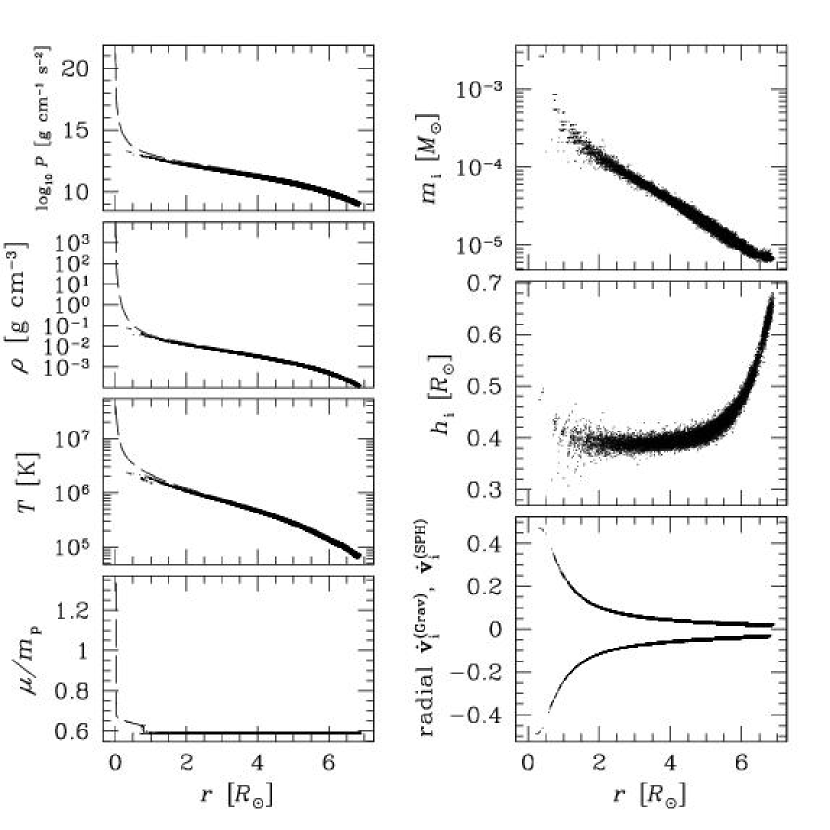
Figure 8: Properties of a $0.9M_{\odot}$ parent star model (RG0.9c) as a function of radius. In the left column (from bottom): mean molecular mass, temperature, density, and base 10 logarithm of pressure. The dashed curves in these four graphs represent the calculated profile of the star, while the points represent our SPH particles. In the right column (from bottom): radial gravitational acceleration (lower curve) and hydrodynamic acceleration (upper curve), smoothing length, and individual particle mass.

5 Results of Collision Simulations

In this section, we report on the results of 32 simulations of parabolic collisions between a subgiant or small red giant and a $1.4M_{\odot}$ NS. The results of these collisions are summarized in Table 2. In terms of computational time, most of the $N=15,780$ particle runs lasted somewhere in the range from 5 to 20 days when run on a typical workstation with a Pentium III or IV processor. As for the three $N=59,958$ particle runs, the $r_{p}=0.96R_{\odot}$ case ran for four weeks and completed its 204 orbits in nearly $7.9\times 10^{4}$ iterations, the $r_{p}=1.91R_{\odot}$ case lasted nearly 6 weeks and completed 219 orbits in more than $1.2\times 10^{5}$ iterations, and the $r_{p}=3.82R_{\odot}$ case took 10 weeks to complete 450 orbits in about $3.25\times 10^{5}$ iterations. When multiple simulations were running, the time per iteration would vary depending on the availability of the MD-GRAPE2 boards: the hydrodynamics was done on separate workstations, but communication with the same host of the MD-GRAPE2 boards was necessary for all calculations.

Figure 9 presents particle plots for one of these collisions, case RG0.9b_RP3.82, in which a $0.9M_{\odot}$ red giant collides with a $1.4M_{\odot}$ NS at a periastron separation of $3.82R_{\odot}$ and an initial separation of $48R_{\odot}$. Frame (a) shows the two bodies just prior to impact. Frame (b) takes place during the first pericenter passage, while frame (c) shows the first apocenter passage. At this time, much of the mass originally bound to the red giant star has been transferred to the NS. Frame (d) occurs during the second pericenter passage, and, approximately twenty hours later, frame (e) occurs during the second apocenter passage. Finally, frame (f) shows a snapshot from the sixth apocenter passage, at a time of 277.5 hr. At this late time, few particles remain bound to the subgiant core.

Table 2: Summary of Collisions

Collision	$r_{\rm p}$	$\Delta M_{c}$	$\Delta M_{NS}$	$M_{3}$	$e$	$a$	$N_{\rm orbit}$
	$(R_{\odot})$	$(M_{\odot})$	$(M_{\odot})$	$(M_{\odot})$		$(R_{\odot})$
(1)	(2)	(3)	(4)	(5)	(6)	(7)	(8)
SG0.8a_RP0.24	0.24	$0.0$	0.013	0.23	0.85	0.24	525
SG0.8a_RP0.48	0.48	$0.0$	0.013	0.20	0.80	0.28	550
SG0.8a_RP0.96	0.96	$0.0$	0.013	0.24	0.64	0.33	334
RG0.8b_RP0.24	0.24	$0.0$	0.005	0.15	0.89	0.65	302
RG0.8b_RP0.48	0.48	$0.0$	0.005	0.11	0.82	0.77	235
RG0.8b_RP0.96	0.96	$0.0$	0.005	0.11	0.70	0.98	207
RG0.8b_RP1.91	1.91	$0.0$	0.005	0.10	0.54	1.26	259
RG0.8b_RP3.82	3.82	$0.0$	0.023	0.07	0.33	2.28	1038
RG0.8c_RP0.24	0.24	$0.0$	0.003	0.15	0.89	0.95	201
RG0.8c_RP0.96	0.96	$0.0$	0.003	0.09	0.71	1.34	281
RG0.8c_RP1.91	1.91	$0.0$	0.003	0.10	0.64	1.78	298
RG0.8c_RP3.82	3.82	$0.0$	0.003	0.06	0.34	2.19	862
RG0.8c_RP5.73	5.73	$0.003$	0.010	0.05	0.18	2.70	1351
RG0.8c_hr_RP0.96	0.96	$0.0$	0.003	0.08	0.62	1.15	204
RG0.8c_hr_RP1.91	1.91	$0.0$	0.005	0.09	0.51	1.62	219
RG0.8c_hr_RP3.82	3.82	$0.003$	0.005	0.08	0.18	2.18	450
SG0.9a_RP0.24	0.24	$0.0$	0.013	0.28	0.92	0.29	371
SG0.9a_RP0.48	0.48	$0.0$	0.013	0.22	0.88	0.33	295
SG0.9a_RP0.96	0.96	$0.0$	0.013	0.34	0.64	0.44	539
SG0.9a_RP1.43	1.43	$0.0$	0.013	0.22	0.53	0.41	288
SG0.9a_RP1.67	1.67	$0.0$	0.013	0.29	0.54	0.46	330
RG0.9b_RP0.24	0.24	$0.0$	0.003	0.18	0.91	0.97	297
RG0.9b_RP0.48	0.48	$0.0$	0.003	0.11	0.85	1.07	531
RG0.9b_RP0.96	0.96	$0.0$	0.003	0.14	0.72	1.26	365
RG0.9b_RP1.91	1.91	$0.0$	0.003	0.12	0.55	1.65	434
RG0.9b_RP3.82	3.82	$0.0$	0.003	0.06	0.43	2.12	1743
RG0.9c_RP0.24	0.24	$0.0$	0.003	0.16	0.94	1.41	261
RG0.9c_RP0.96	0.96	$0.0$	0.003	0.14	0.77	1.67	213
RG0.9c_RP1.91	1.91	$0.0$	0.003	0.10	0.65	2.08	200
RG0.9c_RP3.82	3.82	$0.0$	0.005	0.11	0.49	2.79	325
RG0.9c_RP5.73	5.73	$0.0$	0.005	0.10	0.36	3.17	416
RG0.9c_RP7.64	7.64	$0.0$	0.005	0.12	0.30	3.37	303

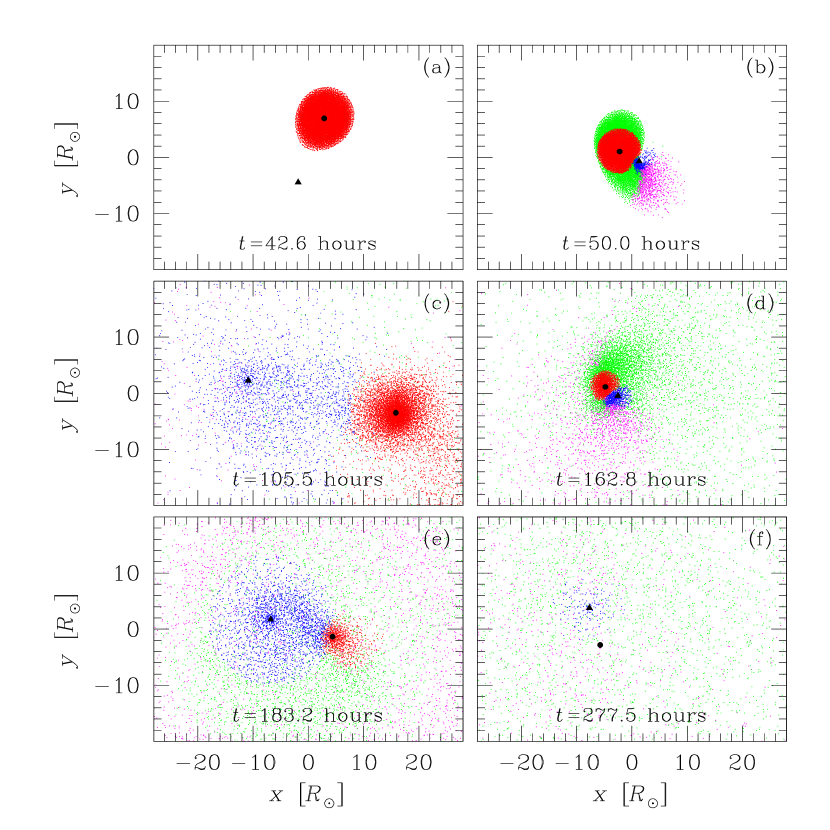
Figure 9: Two-dimensional projections onto the orbital plane of SPH particle and point-mass positions at various times in case RG0.9b_RP3.82. The red giant core is illustrated with a solid circle and the NS with a solid triangle. Particles are colored according to the component to which they are currently considered bound: blue for the NS, red for the red giant core, green for the CE, and magenta for the ejecta.

During all of the stellar collisions we considered, some SPH particles form a CE that surrounds the binary. Various projections of the SPH particles, including those particles in the CE, can be seen in Figure 10 at two different times for case RG0.9b_RP3.82. At 277.5 hr, there are 158 SPH particles considered bound to the NS, 3 SPH particles bound to the subgiant core component, and 4631 particles in the CE. By a time of 12,380 hr, when the simulation is terminated, these numbers have stabilized to 1, 0, and approximately 600, respectively. Although the outer layers of the CE are expanding even at the end of the simulation, this fluid is still gravitationally bound to the binary, with a mass of approximately $0.06M_{\odot}$ in this case.

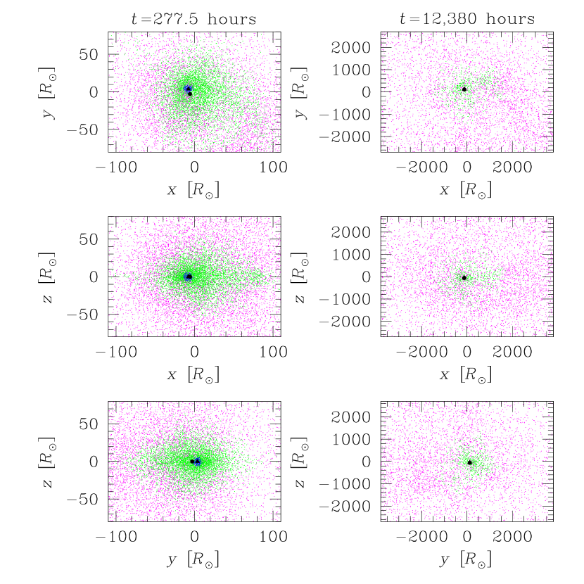
Figure 10: Two dimensional projections of SPH particle and point-mass positions at two select times in the case RG0.9b_RP3.82: the left column is at 277.5 hr, as in frame (f) of Fig. 9, and the right column at 12,380 hr. Particle colors are as in Fig. 9.

Figures 11 and 12 show energies as a function of time for the cases RG0.9b_RP3.82 and RG0.8c_RP0.96, respectively. The sharp oscillating peaks in the total kinetic and potential energy plots correspond to pericenter passages, which become more frequent as the collision progresses. During the late times shown in the right column, the binary has stabilized, and thus the internal energy and frequency of kinetic and potential energy oscillations remain relatively constant.

For our $N=15,780$ runs, the difference between the maximum and minimum total energy is typically $\sim 10^{46}$ erg, at most a few percent of the total energy in the system. Energy conservation in our $N=59,958$ runs is better by a factor of $\sim 2$. We find that decreasing $C_{N,1}$ and $C_{N,2}$ makes energy be conserved even more accurately, but does not significantly affect final masses or orbital parameters. Energy conservation at late times, when the binary is left surrounded by a CE, is typically excellent. The level of energy conservation tends to improve somewhat as we consider more evolved parent stars or larger impact parameters. In all of our runs, angular momentum conservation holds at an extremely high level of accuracy, typically at the $10^{-4}$% level or better. Even in the case of RG0.8c_RP5.73, one of our longest runs, angular momentum is conserved to better than $3\times 10^{-4}$%.

Figure 11: Energies as a function of time for collision RG0.9b_RP3.82. The left column presents the time evolution up to 700 hr. The right column presents a 60 hr time interval much later in the simulation. The gravitational potential energy $W$ curve is the most negative, the total energy $E$ curve is nearly horizontal, the internal energy $U$ curve approaches a small positive energy at late times, and the kinetic energy $K$ curve is the positive one with large fluctuations that are synchronized with the phase of the orbit. These energies do not include the self-energy of the core or NS.

Figure 12: Like Figure 11, but for the collision RG0.8c_RP0.96.

Figure 13 shows component masses and orbital parameters as a function of time for case RG0.9b_RP3.82. By 200 hours (during the third pericenter passage), the subgiant ($M_{2}$) has been nearly completely stripped. This lost mass is transferred to the NS ($M_{1}$), transferred to the CE ($M_{3}$), or, most commonly, ejected to infinity. By the end of the collision, $M_{1}$ is approximately $1.403M_{\odot}$ and the eccentricity $e$ has stabilized near $0.43$.

Figure 13: Masses $M_{i}$, semimajor axis $a$, and eccentricity $e$ as a function of time for collision RG0.9b_RP3.82. The masses $M_{1}$, $M_{2}$, and $M_{3}$ correspond to the masses containing NS, the subgiant core, and the CE gravitationally bound to the binary system, respectively. The dashed vertical lines correspond to the moments of 25, 50, 100, 200, 400, 800, and 1600 completed orbits.

Figure 14 shows the evolution of the component masses and orbital parameters for the collision RG0.8b_RP3.82, a case that we carried out to over 1000 orbits. The perturbation to the orbit near a time of $t=1700$ hours, most easily seen in the eccentricity plot, occurs when the final gas is stripped from the subgiant core. After this time, the orbital parameters for the inner binary are essentially unaffected, although there is a very gradual decrease in the mass $M_{3}$ considered to be in the CE.

Figure 14: Like Fig. 13, but for the collision RG0.8b_RP3.82. The dashed vertical lines correspond to the moments of 25, 50, 100, 200, 400, and 800 completed orbits.

Figure 15 shows the same parameters for the collisions RG0.8c_RP0.96 and RG0.8c_hr_RP0.96. These two cases both involve the same, evolved parent star, but the latter case uses a model with more SPH particles ($N=59,958$ as opposed to $N=15,780$) and a less massive central point particle ($m_{pt}=0.25M_{\odot}$ as opposed to $m_{pt}=0.27M_{\odot}$). In both cases, the relatively small periastron separation leads to an eccentric orbit in which the red giant ($M_{2}$) is stripped of most of the initial mass within 50 hours, leaving only the point particle. As the binary stabilizes, $M_{1}$ remains constant at $1.403M_{\odot}$ in both cases. Although the details of the $M_{3}$ curves differ at early and intermediate times, both cases settle to essentially the same final common envelope mass $M_{3}$ of about $0.08$ or $0.09M_{\odot}$. In the case RG0.8c_RP0.96, the eccentricity $e$ tends toward $0.71$ and the semimajor axis $a$ stabilizes near $1.34R_{\odot}$ at late times, while in the case RG0.8c_hr_RP0.96, these quantities aproach 0.62 and $1.15R_{\odot}$, respectively. These differences in final orbital parameters are largely due to the different $m_{pt}$ values. For a given total mass and impact parameter, the trend is for smaller $m_{pt}$ to yield somewhat less eccentric and tighter orbits: this is true regardless of whether the $m_{pt}$ is smaller because of increased numerical resolution (compare the higher resolution collisions of RG0.8c_hr models with their medium resolution counterparts) or because the parent is in a different evolutionary stage (compare, for example, RG0.8c_RP0.96 and SG0.8a_RP0.96).

By considering plots like those of Figures 13, 14, and 15, we are able to determine final component masses and orbital parameters for all of our calculations (see Table 2 and Fig. 16).

Figure 15: Like Fig. 13 and 14, but for two similar collisions: the thin curve is for RG0.8c_RP0.96 ($N=15,780$ SPH particles and $m_{pt}=0.27M_{\odot}$), while the bold curve is for RG0.8c_hr_RP0.96 ($N=59,958$ and $m_{pt}=0.25M_{\odot}$).

Figure 16: Mass $M_{3}$ of the CE, mass $M_{1}$ of the NS and its bound fluid, final semimajor axis $a$, and final eccentricity $e$ as a function of normalized periastron separation $r_{\rm p}/R$. The left column (open shapes) corresponds to collisions with a $0.8M_{\odot}$ subgiant or giant star and the right column (solid shapes) corresponds to collisions with a $0.9M_{\odot}$ subgiant or giant star. From least to most evolved: SG0.8a and SG0.9a are represented with triangles, RG0.8b and RG0.9b with squares, and RG0.8c and RG0.9c with circles. The symbol $\otimes$ refers to collisions involving our RG0.8c_hr model.

Figure 17: Dependence of the gravitational radiation merger time $\tau_{gw}$ on post-collision semimajor axis $a$ and eccentricity $e$. The points types are as in Fig. 16. The area of the shape is indicative of $r/(dR/dt)$, where $r$ is the rate of collisions for a star of radius $R$, and hence is larger for the less evolved subgiants, which are more likely to be involved in a collision. The dashed curves are curves of constant gravitational merger time, as labelled, for a 1.4 $M_{\odot}$ NS and a $0.25M_{\odot}$ WD. The orbital period $P$ values on the right axis are for these same masses and are calculated simply from Kepler’s third law. The hatched area shows how the $\tau_{\rm gw}=10^{10}\,$yr curve changes when we vary the binary parameters: the upper boundary corresponds to a $1.5\,M_{\odot}$ NS with a $0.45\,M_{\odot}$ WD, and the lower boundary corresponds to a $1.3\,M_{\odot}$ NS with a $0.15\,M_{\odot}$ WD.

6 Discussion and Future Work

We have shown that collisions between NSs and subgiants or small red giants naturally produce tight eccentric NS-WD binaries that can become UCXBs. These results reinforce our findings in Ivanova et al. (2005), where we consider the rate of UCXB formation and show that all currently observed UCXBs could be explained from this channel. In addition, our paper has demonstrated the importance in SPH codes of using the variational equations of motion and simultaneously solving for particle densities and smoothing lengths.

We have found no significant complications applying the variational equations of motion or the simultaneous solution of $\rho_{i}$ and $h_{i}$ in either our one- or three-dimensional hydrodynamics code. Our simple tests of these methods in §3 help demonstrate the significantly improved accuracy of SPH when these approaches are applied together. In particular, the combination of these approaches produces a change in entropy that most closely matches that of known solutions, without disturbing energy conservation. Additional shocktube tests show similar results. The reduction in numerical noise that occurs when particle densities and smoothing lengths are found simultaneously is due to the resulting gradual variation of smoothing lengths from iteration to iteration. Note that if the smoothing lengths are instead determined by requiring that a particle have some desired number or mass of neighbors, then these smoothing lengths can typically take on a range of values. Noise is then introduced by abrupt changes in the smoothing length as neighbors enter or leave the kernel.

In our parabolic collisions of a NS and a subgiant or red giant, we find the stripping of the core to be extremely efficient. In all but two cases, which were both grazing collisions with an evolved $0.8M_{\odot}$ red giant, the core was stripped completely of SPH fluid. We could not, however, resolve the innermost fluid outside the core even in our parent models, and so the best we can do is place an upper limit of $m_{pt}-m_{c}$ (usually $\sim 0.05M_{\odot}$) on the actual amount of mass that would remain bound to the core after the collision. As the radius of the core is about $0.02R_{\odot}$ for all of our (sub)giant parent stars, to resolve the fluid down to the core would require an increase in the number of particles by roughly a factor $(0.02R_{\odot}/a_{1})^{3}$, where the $a_{1}$ values that set the particle spacing are given in the last column of Table 1. Therefore to get the core mass correct for our least evolved $0.8M_{\odot}$ star would require about $2\times 10^{6}$ particles. The other parent stars would require more particles, up to about $2\times 10^{8}$ for our most evolved $0.9M_{\odot}$ RG.

Some of the fluid initially in the sub giant or red giant envelope, from 0.003 to $0.023M_{\odot}$ in the cases we considered, is left bound to the NS. This fluid will likely be accreted onto the NS, potentially recyling it to millisecond periods. By carrying out our collisions between a NS and a subgiant or red giant to many orbits, we were able to identify the existence of a residual, distended CE surrounding a binary consisting of the NS and the subgiant or giant core. The ultimate fate of this diffuse CE is rather uncertain. This gas will likely be quickly ejected by the radiation released by accretion onto the NS. Nevertheless, even a brief CE episode phase will only increase the rate of orbital decay as compared to that from gravitational radiation alone. The gravitational merger timescale therefore provides an upper limit on how long it will take for a UCXB to form.

When we apply the Peters (1964) equations to these post-collision systems, we find that most of them inspiral on rather short timescales (Fig. 17). We conclude that all collisions between a subgiant and a NS, as well as all but the most grazing RG-NS collisions, can produce UCXBs within a Hubble time. As seen in Figure 17, high eccentricities are an important factor in keeping merger times short. However, as discussed in Ivanova et al. (2005), even if all binaries were able to circularize quickly (compared to the gravitational merger time), a large fraction of post-collision systems would still merge in less than the cluster age, as can be seen directly from Figure 17.

If we could run all of our simulations at much higher resolution, we would expect the details of the resulting orbital parameters to change but our conclusions to be unaffected. In particular, higher resolution calculations would allow the point mass $m_{pt}$ to be closer to the true core mass $m_{c}$ and could therefore more accurately determine the mass left bound to the (sub)giant core. Using our three high resolution calculations as a guide, we expect that the resulting eccentricity $e$ and semimajor axis $a$ values of the binary would also be somewhat decreased. However, judging from the shape of the constant $\tau_{gw}$ curves in Figure 17 and the change in $e$ and $a$ that resulted by going from $N=15,780$ to $N=59,958$, we would not expect the gravitational merger time to be dramatically affected. That is, we would still typically be left with a tight, eccentric binary that would merge within a Hubble time.

Bildsten & Deloye (2004) have recently shown that the cutoff in the observed luminosity function of extragalactic LMXBs can be explained if nearly all of the UCXB progenitors consisted of a NS accreting from a compact object with a mass comparable to the helium core mass at turnoff. Our scenario for UCXB formation provides a natural explanation for such progenitors. When our channel for UCXB formation is followed, the donor will be a helium WD, perhaps with small amounts of hydrogen left over from the (sub)giant envelope. It has long been known that the 11.4 minute UCXB 4U 1830-20 contains exactly such a helium donor (Rappaport et al., 1987). Recently, in ’t Zand et al. (2005) have also identified 2S 0918-549 as a likely UCXB with a helium WD donor. Although a subset of UCXBs may contain C-O WD donors (see Juett & Chakrabarty (2005) and references therein), these systems could result from collisions between a NS and an assymptotic giant branch star.

References

- Alexander & Ferguson (1994) Alexander, D. R., & Ferguson, J. W. 1994, ApJ, 437, 879
- Balsara (1995) Balsara, D. 1995, J. Comput. Phys., 121, 357
- Bildsten & Deloye (2004) Bildsten, L., & Deloye, C. J. 2004, ApJ, 607, L119
- Chakrabarty (2005) Chakrabarty, D. 2005, Binary Radio Pulsars, ASP Conf. Ser., Vol. 328, page 279, ed. F.A. Rasio & I.H. Stairs
- Clark (1975) Clark, G.W. 1975, ApJ, 199, L143
- Davies, Benz, & Hills (1992) Davies, M. B., Benz, W., & Hills, J. G. 1992, ApJ, 401, 246
- Deloye et al. (2005) Deloye, C. J., Bildsten, L., & Nelemans, G. 2005, ApJ, 624, 934
- Deloye & Bildsten (2003) Deloye, C.J., & Bildsten, L. 2003 ApJ, 598, 1217
- Freire (2005) Freire, P.C.C. 2005, Binary Radio Pulsars, ASP Conf. Ser., Vol. 328, page 405, ed. F.A. Rasio & I.H. Stairs
- Hernquist (1993) Hernquist, L. 1993, ApJ, 404, 717
- in ’t Zand et al. (2005) in ’t Zand, J. J. M., Cumming, A., van der Sluys, M. V., Verbunt, F., & Pols, O. R. 2005, ArXiv Astrophysics e-prints, arXiv:astro-ph/0506666
- Ivanova et al. (2005) Ivanova, N., Rasio, F. A., Lombardi, J. C., Dooley, K. L., & Proulx, Z. F. 2005, ApJ, 621, L109
- Juett & Chakrabarty (2005) Juett, A. M., & Chakrabarty, D. 2005, ApJ, 627, 926
- Kippenhahn et al. (1967) Kippenhahn, R., Weigert, A., & Hofmeister, E. 1967, Methods in Computational Physics, Vol. 7, ed. B. Alder, S. Fernbach, & M. Rothenberg (New York: Academic), 129
- Kittel (1986) Kittel, C. Introduction to Solid State Physics, Sixth Edition, New York: John Wiley & Sons, Inc., 1986. 1-22.
- Lai, Rasio & Shapiro (1994) Lai, D. Rasio, F. A. & Shapiro, S. L. 1994, ApJ, 423, 344
- Lombardi et al. (1996) Lombardi, J. C., Rasio, F. A., & Shapiro, S. L. 1996, ApJ, 468, 797
- Lombardi et al. (1999) Lombardi, J. C., Sills, A., Rasio, F. A., & Shapiro, S. L. 1999, J. Comp. Phys., 152, 687
- Monaghan (1989) Monaghan, J. J. 1989, Journal of Computational Physics, 82, 1
- Monaghan (2002) Monaghan, J. J. 2002, MNRAS, 335, 843
- Monaghan & Lattanzio (1985) Monaghan, J. J. & Lattanzio, J. C. 1985, Astron. and Astrophys., 149, 135
- Nelson & Papaloizou (1993) Nelson, R. P. & Papaloizou, J. C. B. 1993, MNRAS, 265, 905
- Nelson & Papaloizou (1994) Nelson, R. P. & Papaloizou, J. C. B. 1994, MNRAS, 270, 1
- Peters (1964) Peters, P.C. 1964, Phys. Rev., 136, 1224
- Podsiadlowski et al. (2002) Podsiadlowski, Ph., Rappaport, S., & Pfahl, E. 2002, ApJ, 565, 1107
- Pooley et al. (2003) Pooley, D., et al. 2003, ApJ, 591, L131
- Press et al. (1992) Press, W. H., Teukolsky, S. A., Vetterling, W. T., & Flannery, B. P. 1992, Numerical Recipes in Fortran, Second Edition, Cambridge University Press.
- Pylyser & Savonije (1988) Pylyser, E., & Savonije, G.J. 1988, A&A, 191, 57
- Rappaport et al. (1987) Rappaport, S., Ma, C. P., Joss, P. C., & Nelson, L. A. 1987, ApJ, 322, 842
- Rasio (1991) Rasio, F. A. 1991, PhD Thesis, Cornell University
- Rasio et al. (2000) Rasio, F.A., Pfahl, E.D., & Rappaport, S. 2000, ApJ, 532, L47
- Rasio & Lombardi (1999) Rasio, F. A., & Lombardi, J. C. 1999, J. Comp. App. Math., 109, 213
- Rasio & Shapiro (1991) Rasio, F. A. & Shapiro, S. L. 1991, ApJ, 377, 559
- Rogers & Iglesias (1992) Rogers, F. J., & Iglesias, C. A. 1992, ApJS, 79, 507
- Serna et al. (1996) Serna, A., Alimi, J.-M. & Chièze, J.-P. 1996, ApJ, 461, 884
- Serna, Domínguez-Tenreiro, & Sáiz (2003) Serna, A., Domínguez-Tenreiro, R., & Sáiz, A. 2003, ApJ, 597, 878
- Sills et al. (2001) Sills, A., Faber, J. A., Lombardi, J. C., Rasio, F. A., & Warren, A. R. 2001, ApJ, 548, 323
- Sills & Lombardi (1997) Sills, A. & Lombardi, J. C. 1997, ApJ, 484, L51
- Sills et al. (1997) Sills, A., Lombardi, J. C., Jr., Demarque, P. D., Bailyn, C. D., Rasio, F. A., & Shapiro, S. L. 1997, ApJ, 487, 290
- Sod (1978) Sod, G. A. 1978, J. Comput. Phys. 27, 1 (1978).