Simulating galaxy clusters – I. Thermal and chemical properties of the intra-cluster medium

Abstract

We have performed a series of N-body/hydrodynamical (TreeSPH) simulations of clusters and groups of galaxies, selected from a cosmological volume within a $\Lambda$CDM framework: these objects have been re-simulated at higher resolution to $z$=0, in order to follow also the dynamical, thermal and chemical input on to the ICM from stellar populations within galaxies. The simulations include metallicity dependent radiative cooling, star formation according to different IMFs, energy feedback as strong starburst-driven galactic super-winds, chemical evolution with non-instantaneous recycling of gas and heavy elements, effects of a meta-galactic UV field and thermal conduction in the ICM.

In this Paper I of a series of three, we derive results, mainly at $z=0$, on the temperature and entropy profiles of the ICM, its X-ray luminosity, the cluster cold components (cold fraction as well as mass–to–light ratio) and the metal distribution between ICM and stars.

In general, models with efficient super-winds (produced by the action of supernovæ and, in some simulations, of AGNs), along with a top-heavy stellar IMF, are able to reproduce fairly well the observed $L_{X}-T$ relation, the entropy profiles and the cold fraction: both features are found to be needed in order to remove high-density and low-entropy cold gas at core scales, although additional alternative feedback mechanisms would still be required to prevent late time central cooling flows, and subsequent overproduction of stars and heavy elements at the centre. Observed radial ICM temperature profiles can be matched, except for the gradual decline in temperature inside of $r\sim$ 0.1$R_{\rm{vir}}$. Metal enrichment of the ICM gives rise to somewhat steep inner iron gradients; yet, the global level of enrichment compares well to observational estimates when a top–heavy IMF is adopted, and after correcting for the stars formed at late times at the base of the cooling flows, the metal partition between stars and ICM gets into good agreement with observations. The overall abundance and profile of iron in the ICM is found essentially unchanged from $z=1$ to present time. Finally, the $\frac{\alpha}{Fe}$ of the gas is found to increase steadily with radius, decreasing over time.

1 Introduction

Clusters of galaxies play a major role in most of the attempts at reconstructing the cosmological history of the Universe. Numerical simulations (since Evrard 1990, and then Thomas & Couchman 1992, Katz & White 1993, Cen & Ostriker 1994, Navarro et al. 1995, Evrard et al. 1996, Eke et al. 1998, Thomas et al. 2002, Tornatore et al. 2003, Borgani et al. 2004) are a powerful tool for making predictions on their formation and evolution, provided that the underlying physical mechanisms are fully taken into account.

In particular cosmological simulations have helped to reproduce many of the X-ray properties of the intra–cluster medium (ICM), which is a hot (1-10 keV) tenuous ($10^{-4}-10^{-2}$ cm^-3), optically thin gas containing completely ionized H and He and partially ionized heavier elements ( “metals”). Metal lines revealed to populate spectra of both groups and clusters, corresponding to metallicities of about 0.2 to 0.4 in solar units, which indicates a non purely primordial origin of the ICM, a fraction of which must have previously been processed in galaxies as inter–stellar medium (ISM) and then transported whence into the space between galaxies.

The ICM is emitting radiation at X-ray wavelenghts by losing energy according to a cooling timescale $t_{cool}\propto\sqrt{T}/n$. In the very central region of many clusters the gas density becomes high enough to make the cooling time shorter than a Hubble time, forming thus a cooler core (typically $R_{c}\sim$100 kpc or more) which affects the gas central density, temperature and entropy distributions (see Sections 3, 4, 5). The ICM has likely been heated up to X-ray emitting temperatures mainly by means of gravitational energy converted to thermal when falling onto the cluster’s potential well. Indeed the basic scenario describing the thermal behaviour of the ICM calls for a gravity-only driven ongoing heating of the gas by adiabatic compression, followed by hydrodynamical shocks arisen during the settling of infalling material. The hot gas will emit mainly by thermal (free-free) Bremsstrahlung, resulting in the simple, theoretical clusters X-ray scaling relations: luminosity–temperature $L_{X}\propto T^{2}(1+z)^{3/2}$, entropy–temperature $S\propto T(1+z)^{-2}$, virial mass–temperature $M\propto T^{3/2}$.

It is by now well known how this simple model basically fails in reproducing the actual scaling properties observed: in fact, the $L_{X}-T$ relation at $z=0$ is steeper than predicted, breaking possibly into two different slopes (see Section 6). As for the S-T relation, an entropy excess with respect to the self-similar expectation has been reported in the inner region of poorer and cooler systems, reaching a constant value (“entropy floor”), likely resulting from softer gas density profiles in the core (Section 5). Finally the M-T relation has been found to have a lower normalization than predicted by “adiabatic” models and simulations of up to $\sim 40\%$.

Physical mechanisms able to explain the break of self–similarity in the properties of the ICM have been extensively proposed during last ten years, and mainly fall in two broad classes: a) non–gravitational heating and b) radiative cooling. Introducing gas cooling and star formation induces gas condensation at core scales, leading to star concentration associated with the central galaxy (cD) which will be dominating the baryonic cluster mass in the core at $z=0$. This affects also the dark-matter (DM) density profile in the core, which steepens from $r^{-1.5}$ to $r^{-2}$. Moreover, inflows of high–entropy gas from extra–core regions are stimulated by virtue of baryon cooling, while lower-entropy, shorter-cooling time gas gets selectively removed from the centre, thus giving rise to an increased level of entropy inside the core itself (Voit & Bryan 2001). On the other hand X-ray luminosity is suppressed since the amount of gas populating the hot diffuse phase gets reduced (Pearce et al. , 2000). However all cluster simulations with cooling and star formation reveal a significant drawback: cooling alone makes a large fraction (30 up to 55%) of gas get converted into a cold phase (either cold gas or stars) within the virial radius at $z=0$ (Suginohara & Ostriker 1998, Balogh et al. 2001, Davè et al. 2001), in contradiction with a value of 10-20% of the baryon fraction locked into stars indicated by observations.

Thus, additional sources of non-gravitational heating are required to counterbalance over–cooling in the cluster’s core, to enhance the entropy of the gas and to suppress its X-ray emissivity (Evrard & Henry 1991, Bower 1997, Lewis et al. 2000, Bialek et al. 2001). One solution would be to appeal to pre–heating, namely episodic mechanisms such as an impulsive injection of energy to all gas particles at redshift high enough to occur either before (external pre–heating: requires less energy to reach a given entropic level because occurring in a less dense pristine environment: e.g. Kaiser 1991, Cavaliere et al. 1997, Balogh et al. 1999, Mo & Mao 2002), or during the gravitational collapse onto the cluster’s potential, or shock heating during late accretion within DM haloes (internal pre–heating: e.g. Tozzi & Norman 2001, Babul et al. 2002, Voit et al. 2003): its effect would be clearly stronger for colder systems (groups and small clusters), where both excess of inner entropy and a steeper L-T relation can be achieved (Cavaliere et al. 1998, Brighenti & Mathews 2001, Borgani et al. 2001).

Feedback processes subsequent to star formation, namely supernovæ induced galactic winds, are natural mechanisms working at both pre–heating and especially metal enriching the ICM (Loewenstein & Mushotzky 1996, Renzini 1997, Finoguenov & Ponman 1999, Wu et al. 2000, Lloyd-Davies et al. 2000, Kravtsov & Yepes 2000, Menci & Cavaliere 2000, Bower et al. 2001, Pipino et al. 2002, Kapferer et al. 2006); yet doubts have been raised as to the actual efficiency in thermalizing the amount of additional supernova energy, which would be maximized e.g. in starbursts. Domainko etal (2004) took into account the effect of heating and metal enrichment from intra-cluster SNe, the energy from which may inhibit or delay the formation of cooling flows, provided that the inter-galactic star fraction is as considerably high as shown in other simulations ($\;\stackrel{{\scriptstyle\textstyle>}}{{\sim}}\;$20-25%, see Sommer-Larsen, Romeo and Portinari, 2005, hereinafter Paper III). Up to now the most promising candidates to supply energy for heating are AGNs associated with quasars, which can have at their disposal huge energetic reservoirs to be converted into gas thermal energy (Bower 1997, Valageas & Silk 1999ab, Wu et al. 2000, McNamara et al. 2000, Yamada & Fujita 2001; Cavaliere, Lapi & Menci 2002, Croton et al. 2006). In conclusion, stellar feedback and/or additional pre–heating must play together with gas cooling to regulate the latter such as to suppress over–cooling (see Pearce et al. 2000, Kay et al. 2003): this will set up the fraction of baryons cooled out (“cold fraction”) to form stars and cold clouds, which in turn drives the distribution of gas density, temperature and entropy.

So far few hydrodynamical simulations have been performed which were able to pursue at the same time and in a self–consistent way the target of realistically modelling the ICM dynamics by including both non-gravitational heating/cooling (complete with feedback/star formation) and the metal enrichment associated with star formation and stellar evolution: Borgani et al. (2001 and 2002), Tornatore et al. (2003), McCarthy et al. (2004) (all though without following metal production from star formation), and especially Valdarnini (2003), Tornatore et al. (2004) and, very recently, Scannapieco et al. (2005) and Schindler et al. (2005).

The physical processes implemented in our simulations and the numerical details are described in Section 2. In Section 3 to 6 we discuss distribution and scaling of density, temperature, entropy and luminosity of the X–ray emitting gas. In Section 7 and 8 we discuss the relation of the hot gas with the cold stellar component and the consequent chemical enrichment. Finally, in Section 9 we draw some summary and conclusions.

2 The Code and Simulations

The cosmological N-body simulation has been performed using the FLY code (Antonuccio et al. , 2003) for a $\Lambda$CDM model ($\Omega_{0}$=0.3, $\Omega_{\Lambda}$=0.7, $\Omega_{b}$=0.04, $h=0.7$, $\sigma_{8}$=0.9) with $128^{3}$ collisionless DM-only particles filling an initial box of 150$h^{-1}$ Mpc at an initial redshift $z_{i}=39$. The gravitationally bound DM haloes at $z$=0 were identified by a FOF group-finder, with a fixed linking length (at $z$=0) equal to 0.2 times the average initial interparticle distance (see e.g. Eisenstein & Hut 1998).

Two small groups, two large groups and two clusters were sorted out from the cosmological simulation, resampled to higher resolution and resimulated by means of an improved version of the Tree-SPH code described in Sommer-Larsen, Götz & Portinari (2003; hereinafter SLGP). We named the two clusters after “Virgo” and “Coma”, because of their virial size: $\sim 3$ and $\sim 6$ keV in terms of X-ray temperature (see table 1), respectively (actually “Coma” rather resembles a “mini-Coma”-like system, being the real Coma at about 8 keV). For each object, all DM particles within the virial radius at $z=0$ have been traced back to the initial condition at $z_{i}$, where the resolution in this “virial volume” has been increased (see below) and one SPH particle has been added per each DM one, with a mass of $m_{SPH}=f_{b}\cdot m_{DM}^{0}$, resulting in a reduced dark-matter mass $m_{DM}=(1-f_{b})\cdot m_{DM}^{0}$: here and throughout this series of papers we have used a baryon mass fraction $f_{b}=\frac{m_{SPH}}{m_{DM}+m_{SPH}}=0.12$, generally consistent with $\Omega_{b}h^{2}$ from nucleosynthesis and cluster observational constraints. The mass resolution reached inside the resampled lagrangian subvolumes from the cosmological set was such that $m_{DM}=1.8\cdot 10^{9}h^{-1}M_{\odot}$ and $m_{g}=m_{*}=2.5\cdot 10^{8}h^{-1}M_{\odot}$ (the mass of star particles equals that of SPH gas particles throughout the simulation, see Section 2.3). In one high-resolution run of the “Virgo” cluster, it was $m_{DM}=2.3\cdot 10^{8}h^{-1}M_{\odot}$ and $m_{g}=m_{*}=3.1\cdot 10^{7}h^{-1}M_{\odot}$. In the surrounding region of these subvolumes the DM particles were increasingly resampled at coarser resolution with increasing radial distance (see Gelato & Sommer-Larsen, 1999), leaving a buffer layer in between at intermediate resolution. As a final configuration, we have therefore an inner region corresponding to the initial virial volume and containing the highest-resolution (64 times the basic value; 512 times for the high resolution run) DM and SPH particles, a buffer region of DM only particles at 8 times resolution, and finally an outer envelope of DM only particles at base resolution.

Softening lenghts controlling gravitational interactions among particles are $\epsilon_{DM}=5.4h^{-1}$kpc and $\epsilon_{g}=\epsilon_{*}=2.8h^{-1}$ kpc (for the high-resolution run: 2.7 and 1.4 $h^{-1}$kpc, respectively); they were kept constant in physical space (meaning increasing with z in comoving coordinates) since $z=6$ and conversely fixed in comoving coordinates at earlier times. These values of the softening lengths for the DM particles correspond to a virial mass of $3.66\cdot 10^{7}h^{2}M_{\odot}$, about two orders of magnitude less than the minimum mass of our particles, which ensures that the gravitational potential is well reproduced even within gravitationally bound groups.

The selected objects’ characteristics are listed in Tables 1 and 2; they have all been chosen such as not to be undergoing any major merger events since $z\sim 1$.
The adopted TreeSPH code schematically includes the following features (see Table 3):

• solution of entropy equation (rather than of thermal energy)

• metal-dependent atomic radiative cooling

• star formation

• feedback by starburst (and optionally AGN) driven galactic winds

• chemical evolution with non-instantaneous recycling of gas and heavy elements (H, He, C, N, O, Mg, Si, S, Ca, Fe)

• thermal conduction

• meta-galactic, redshift-dependent UV field.

In the following subsections we describe in more details how star formation and feedback mechanisms work, and how we implement chemical evolution with cooling.

2.1 Star Formation and Feedback as Super-Winds

Although only a minor fraction of the baryons in groups and clusters is in the form of stars and cold gas, the ICM is significantly enriched in heavy elements, with an iron abundance about 1/3 solar in iron (e.g. Arnaud et al. 2001; De Grandi & Molendi 2001; De Grandi et al. 2004; Tamura et al. 2004, to quote a few recent BeppoSAX and XMM studies). In fact one can show from quite general arguments that at least half and probably more of the iron in galaxy clusters resides in the hot ICM with most of the remaining iron locked up in stars (Renzini et al. 1993; Renzini 1997, 2004; Portinari et al. 2004). Moreover, observations of galaxy clusters up to $z$$\sim$1 indicate that the ICM metals were already widely in place at this redshift (Tozzi et al. 2003).

Since the metals must have mainly or exclusively been manufactered in galaxies (whether still existing or by now disrupted into an intra–cluster stellar population), efficient gas and metals outflows from these must have been substantially at work in the past ($z$$\ga$1): we shall in the following denote these “galactic super-winds”, and SW simulations those run with such strong wind feedback. The galactic super-winds may be driven by supernovæ or hypernovae (e.g. Larson 1974, Dekel & Silk 1986, Mori et al. 1997, Mac Low & Ferrara 1999, SLGP), AGNs (e.g., Silk & Rees 1998; Ciotti & Ostriker 1997, 2001; Romano et al. 2002; Springel, Di Matteo & Hernquist 2005; Zanni et al. 2005), or a combination of the two.

Recent work on galaxy formation indicates that in order to get a significant population of disc galaxies with realistic properties in addition to steady, quasi self-regulated star formation, one has to invoke early non-equilibrium outflow processes (e.g., Abadi et al. 2003, SLGP, Governato et al. 2004, Robertson et al. 2004). Such early star-burst driven outflows were incorporated in the simulations of SLGP, and in the present simulations we build on this approach, except that in general we allow such outflows to occur at all times (all “SW” runs: see below).

Specifically our approach is the following: cold gas particles ($T$$<$$2\cdot 10^{4}$K) are triggered for star formation on a timescale $t_{*}=t_{dyn}/\epsilon_{SF}$ (where the star formation efficiency $\epsilon_{SF}=0.02$) if the gas density exceeds a certain critical value, chosen to be $n_{\rm{H}}^{up}=1.0$ cm^-3; we have experimented with other values and found that the outcome of the simulations is very robust with respect to changes in this parameter. To model the sub-resolution physics of star-bursts and self propagating star formation in a simplistic way we assume that, if a SPH particle satisfies the above criterion and has been triggered for star formation, then with a probability $p_{\rm{burst}}$ its neighbouring cold and dense SPH particles with densities above $n_{\rm{H}}^{low}(<n_{\rm{H}}^{up})$ are also triggered for star formation on their respective dynamical time scales. The fraction $f_{\rm{wind}}$ of all stars formed which partake in bursts is controlled through the parameters $n_{\rm{H}}^{low}$ and $p_{\rm{burst}}$. Simulations with combinations of the latter two parameters yielding similar values of $f_{\rm{wind}}$ give similar results, so effectively the wind “strength” is controlled by one parameter. For most simulations presented in this paper we have used $n_{\rm{H}}^{low}=0.8$ cm^-3 and $p_{\rm{burst}}$=0.1, resulting in $f_{\rm{wind}}$$\simeq$0.8.

When a star particle is born, it is assumed to represent a population of stars formed at the same time in accordance with a Salpeter or an Arimoto-Yoshii (Arimoto & Yoshii, 1987) IMF. It feeds energy back to the local ISM by Type II supernovæ (SNII) explosions during the period 3-34 Myr after formation: in fact, the lightest stars which contribute feedback from SNII explosion have a mass of about 9 $M_{\odot}$ and lifetimes of about 34 Myr; and the upper limit of the IMF is assumed to be 100 $M_{\odot}$ corresponding to a lifetime of about 3 Myr (see Lia, Portinari & Carraro 2002). Stars with masses greater than 9 $M_{\odot}$ are assumed to deposit $\sim$ 10⁵¹ ergs per star to the ISM as they explode as SNII. Throughout, the energy output from stellar winds is neglected, because even for metal-rich stars it is an order of magnitude less than the output from SNII.

SNII events are associated with multiple explosions of coeval stars in young stellar (super-)clusters, hence resulting in very efficient contribution to energy feedback. In the simulations, the energy from SN II is deposited into the ISM as thermal energy at a constant rate during the aforementioned period (the energy is fed back to the, at any time, 50 nearest SPH particles using the smoothing kernel of Monaghan & Lattanzio 1985). Part of this thermal energy is subsequently converted by the code into kinetic energy as the resulting shock-front expands. While a star particle is feeding energy back to its neighbouring SPH particles, radiative cooling of these is switched off: this is an effective way of modelling with SPH a two-phase ISM consisting of a hot component ($T\sim 10^{6}-10^{7}$ K) and a much cooler component ($T\sim 10^{4}$ K) — see Mori et al. M.97 (1997), Gerritsen G97 (1997) and Thacker & Couchman (2000 and 2001). At the same time interrupting cooling in the surrounding region of star particles undergoing SNII explosion, helps mimicking the adiabatic phase of expansion, thus creating super-shells. Such an adiabatic phase of supernovæ explosion would be missed in the simulations if the whole thermal energy released were to get dissipated by efficient cooling mechanisms. The feedback related to the (non star-burst) conversion of individual, isolated SPH particles to star particles typically results in “fountain-like” features, and does not lead to complete “blow-away”.

In fact, a typical star-burst event as described above gives origin to 40-50 star particles which are at formation localized in space and time. The energy feedback from these star particles drives strong shocks/“super-shells” outwards through the surrounding gas, sweeping up gas and metals and transporting these to (and mixing into) the ICM — such outflows being the “galactic super-winds” we introduced. These super-winds are quite well resolved numerically — a further improvement in the present work has been the adoption of the “conservative” entropy equation solving scheme of Springel & Hernquist (2002), which improves shock resolution over classic SPH codes.

The amount of energy injected into the Inter Stellar Medium (ISM) by Type II supernovae per unit mass of stars initially formed can be expressed as $\propto f_{\rm{AGN}}~{}\beta~{}\nu_{SN}~{}E_{SN}$, where $f_{\rm{AGN}}$ normally is unity (but see below), $\beta\leq 1$ accounts for possible radiative losses, $\nu_{SN}$ is the number of Type II supernovae produced per unit mass of stars formed and $E_{SN}$ is the amount of energy released per supernova. For this work we assume $\beta E_{SN}$=10⁵¹ ergs. The parameter $\nu_{SN}$ depends on the IMF: for the Salpeter IMF $\nu_{SN}=6\times 10^{-3}$, for the Arimoto-Yoshii IMF $\nu_{SN}=1.5\times 10^{-2}$, corresponding to 6 and 15 SNII respectively (from progenitors with $M\geq 9~{}M_{\odot}$), per 1000 M_⊙ of stars formed. To mimic the effect of possible additional feedback from central, super-massive black holes in a very crude way we set in some simulations $f_{\rm{AGN}}$=2 or 4 (SWx2 and SWx4 runs respectively), on the basis of the hypothesis that AGN activity mirror star formation (Boyle & Terlevich 1998).

As a test of reference, one set of simulations (“WFB”) were run with early super-winds only, as SLGP assumed for modelling individual galaxies. This resulted in a very small (average) value of $f_{\rm{wind}}$=0.07, and a consequent very low level of enrichment of the ICM. As a result, this WFB set has been run using an approximately primordial cooling function in the ICM, and hence is similar to most of the previously attempted simulations performed without metal production from star formation and subsequent chemical evolution of the ICM (e. g. Tornatore et al. , 2003).

The above “super-wind” scheme is not resolution independent by construction, yet simulations at 8 times higher mass and twice better force resolution give similar results (see e.g. Section 6 and also Paper II), indicating that the scheme is effectively resolution independent. Although the above scheme is just a simplistic way of modeling galactic outflows, it has the advantage that such outflows are numerically resolved, and that the gas dynamics of the outflow process is self-consistently handled by the code.

Finally, Type Ia supernovæ (SNIa) are also implemented in the simulations as sources of chemical enrichment. However,since SNIa explosions are considerably less numerous than SNII (per unit mass of stars initially formed), and also are typically uncorrelated in space and time, we neglect their energy feedback in the current simulations. As a matter of fact, SNIa explosions, occurring in low-density environments, may be in principle more efficient in contributing to feedback (Recchi, Matteucci & D’Ercole 2001; Pipino et al. 2002); nonetheless they represent isolated events not giving rise to cumulative, large scale effects such as the supershells resulting from correlated SNII explosions.

Table 1: Structural properties of selected clusters and groups at $z$=0

Cluster #	$M_{vir}$	$R_{vir}$	$<kT_{ew}>$ a
	[1014M⊙]	[Mpc]	[keV]
“Coma”	12.38	2.90	6.00
“Virgo”	2.77	1.77	3.06
202	1.25	1.29	2.24
215	1.03	1.18	1.48
550	0.48	0.96	1.00
563	0.49	0.94	1.10
a Temperatures referred to the ”standard” run AY-SW

Table 2: Numerical properties of the simulations. All the runs were started from initial redshift $z_{i}$=19, except “Virgo” high-resolution, for which $z_{i}$=39; throughout the paper, all results from the latter refer to $z=0.07$, up to which the simulation has actually run as of submission date. Last two columns refer to SW runs.

Cluster #	$N_{DM}$	$N_{SPH}$	$N_{DM}^{z=0}$	$N_{SPH+*}^{z=0}$
			$(r<R_{vir})$	$(r<R_{vir})$
“Coma”	517899	429885	356300	330850
“Virgo”	148634	109974	82461	75918
“Virgo”x8	1140731	1093992	707500	646547
202	69330	52192	40900	36230
215	62265	46294	30950	27490
550	51392	33734	16875	13667
563	44872	28056	15800	13760

Table 3: Characteristics of the runs: all implement the SW scheme ($\epsilon_{SF}=0.02$, $f_{wind}=0.8$), except Sal-WFB and ADIAB

#	$IMF$	$f_{AGN}$	$f_{wind}$	preh.@ z=3
				[keV/part.]
AY-SW	AY	1	0.8	0
AY-SWx2	AY	2	0.8	0
AY-SWx4	AY	4	0.8	0
PH0.75	AY	1	0.8	0.75
PH1.50	AY	1	0.8	1.50
PH50	AY	1	0.8	50 $\cdot$ cm2
Sal-SW	Sal	1	0.8	0
Sal-WFB	Sal	1	0.07	0
COND	AY	1	0.8	0
ADIAB	–	–	–	0

2.2 Cooling flow correction

The simulations show active star formation, induced by strong cooling flows, at the very centre of the cD galaxies down to $z=0$, which has no counterpart in observed clusters; such spurious late activity is responsible for a non negligible fraction of the cluster stellar mass and these young stellar populations would significantly contribute to the total luminosity. Therefore a correction must be applied, if aiming at reproducing observed quantities such as cold fraction, star formation rate as well as the metal production and distribution in the ICM (see Sections 7 and 8; also Paper III and D’Onghia et al. 2005).

Specifically, our correction consists in selecting and subtracting out the star particles formed within the innermost 10 kpc since some $z_{corr}$: as the main epoch of general galaxy formation in the clusters is over by $z\sim 2$ (see Paper II), we assume $z_{corr}$=2 as the redshift below which spurious central star formation induced by cooling flows can be neglected; we also verified that the correction is quite stable for $z_{corr}$ up to 2.5.

2.3 Chemical evolution

There is a deep interconnection between chemical and hydrodynamical evolution when addressing metal production and mixing into the ICM. Stars return to the surrounding ISM part of their mass, including chemically processed gas, and of their energy (stellar feedback): the whole star formation process acts onto the cluster gas evolution both through energy feedback from supernovæ (see previous section), counteracting the cool-out of the hot gas, and through metal enrichment of the ICM, which instead boosts its cooling rate. The rates of release of both energy (SN rate) and metals are set by the IMF, which also regulates the returned fraction from the stellar to the gaseous phase: in a Salpeter distribution, 30% of the stellar mass formed is returned to the gaseous phase within a Hubble time, whilst in an Arimoto-Yoshii (AY) distribution the returned fraction is about 50%.

In our simulations, star formation and chemical evolution are modelled following the “stochastic” algorithm of Lia et al. (2002; hereinafter LPC). When a cold gas particle is selected for star formation, it is entirely transformed to a star particle with a probability given by the star formation efficiency. The new-born collisionless star particle hosts a Single Stellar Population (SSP), namely a distribution of stellar masses (according to the chosen IMF) all coeval and with homogeneous chemical composition, which is the composition of the gas particle that switched to a star particle. During its lifetime, such a SSP will release gas and metals (both newly synthesized and original ones). The return of gas and metals to the interstellar medium is also modelled stochastically, and a star particle will entirely “decay”, or “return” back to be a SPH collisional particle, with a probability given by the returned fraction of the corresponding IMF. Which is to say, in simulations with the Salpeter IMF 30% of the star particles will return to be gas in a Hubble time, while with the AY IMF 50% of the star particles decay back to gas particles, overall. Notice that the decay is not instantaneous: only 10% (for Salpeter, 30% for AY) of the SSP mass is returned to the ISM in the initial burst phase (the initial 34 Myr, Section 2.1), the rest of the decay of the star particles occurs spread over a Hubble time. According to its age, a decaying star particle carries along to the gaseous phase the metals produced by the SSP in that time window (namely, the products of the dying stars and exploding supernovæ with the corresponding lifetime). Thus the algorithm follows non–instantanoues gas recycling, as well as the corresponding delayed metal production. In particular, mass loss and metal production from intermediate and low mass stars, and the delayed chemical enrichment from SNIa, are accounted for. The algorithm follows the evolution of H, He, C, N, O, Mg, Si, S, Ca and Fe. Full details of the algorithm can be found in LPC. Among the advantages of this algorithm, the number of baryonic particles and their mass is conserved throughout the simulation: since they switch from gas to stars, and back from stars to gas, in their entirety with no splitting, $m_{*}=m_{SPH}$ always.

Some modifications have been applied to the original LPC algorithm, to adapt it to our “starburst and supershell” feedback scheme described in the previous section. In the first 34 Myrs, i.e. during the starburst phase, the energy and metals released from massive stars are not implemented statistically; rather, with the rates predicted by the corresponding IMF, there is a steady release of energy and metals over the neighbouring gas particles, hence the expanding super-shell is also enriched in metals. When reaching 34 Myr, a fraction of the star particles responsible for the burst are turned to SPH particles, with the suitable probability to describe the actual returned gas fraction at that age (about 10% or 30% for the Salpeter or AY IMF, see above). Only from 34 Myrs onwards, metal production is treated with the stochastic approach of LPC. Being limited to the very early, short stages of the SSP lifetime, this modification does not hamper the correct modelling of delayed gas recycling and metal production achieved with the LPC algorithm; but it allows a better connection between energy and metal feedback from SNII in our starburst models, and a more efficient transport of the SNII metals outward by the expansion of the corresponding supershell.

Further mixing of the metals, both the SNII metals and those released by later decay of star particles, could be due to metal diffusion. In LPC, metal diffusion was taken into account with a diffusion coefficient $\kappa$ based on the expansion of individual supernova remnants; this is relevant for modelling galactic scales, but can be neglected on cluster scales. Besides, in our simulations the diffusion related to the expansion of (multiple) SN shells is implicit in the treatment of the winds. Hence in our present simulations we neglect (additional) metal diffusion ($\kappa$=0).

2.4 Background UV field and metal-dependent cooling

A source of radiative heating is provided by a homogeneous and isotropic UV background radiation field switched on at $z=6$ and modelled after Haardt & Madau (1996), to integrate the effect of sources such as AGNs and/or young blue galaxies. The presence of a UV field affects galaxy formation only at low temperatures, which is the case at the beginning of the process, when also heating by photo–ionization is important. Moreover, at the typical densities of strongly cooling, galaxy forming gas ($n_{H}\raisebox{-3.8pt}{$\;\stackrel{{\scriptstyle\textstyle>}}{{\sim}}\;$}10^{-2}$ cm^-3), the primordial abundance cooling function is only significantly modified by a UV field of this kind at temperatures log$T\raisebox{-3.8pt}{$\;\stackrel{{\scriptstyle\textstyle<}}{{\sim}}\;$}4.5$, even at epochs when the UV intensity is largest ($z=2-3$).

The radiative cooling rate of atomic gas closely depends on its chemical composition, whose evolution is followed in detail in the simulations (Section 2.3); in general, this dependence acts in such a way that, at a given density, the cooling efficiency increases for higher metallicity, leading to accelerated star formation. Including effects owing to metal line cooling is thus decisive for modelling in a realistic way the transformation of baryons into stars, and hence the whole history of galaxy formation (see Scannapieco et al., 2005).

We take metal–dependent cooling consistently into account in the simulations, by means of the cooling functions of Sutherland & Dopita (1993: SD): in such a way the cooling process of the gas takes place accordingly to its metal content, as resulted from the enrichment described in the previous subsection. With respect to a primordial composition of only H and He, metals in the gas affect its cooling rate mainly at temperatures $logT\raisebox{-3.8pt}{$\;\stackrel{{\scriptstyle\textstyle>}}{{\sim}}\;$}4.5$: since the effects of the adopted UV field and of metal cooling are relevant in different temperature ranges (below and above $logT\simeq 4.5$, respectively), to a first approximation they can be treated as independent corrections to the primordial abundance cooling function.

Radiative cooling is a function of the local metal abundance, calculated by the standard smoothing kernel of our code: though the metals are not spread around by diffusion, the cooling function is computed basing on the average metallicity of all neighbouring gas particles, also in order to avoid overestimating cooling from particles with high $Z$.

The adopted metal–dependent cooling functions of SD are given for chemical compositions mimicking those in the Solar Vicinity (from solar–scaled to $\alpha$–enhanced at low metallicities). In general, the mixture of metals in the simulations (as well as in real astrophysical objects) does not necessarily follow the same trends as the local one. Ideally, one would need cooling functions for different compositions (different relative proportions of different elements) since the cooling contribution from different elements, different ionization stages and different lines, depends on temperature and a global scaling with metallicity is never a perfect description. However, this is not yet possible so we link the available cooling functions to the actual composition of our gas particles, basing on the global abundance of metals by number; in fact, what matters for the cooling efficiency is the number of coolants (metal atoms and ions), rather than the abundance of metals by mass (the “metallicity” $Z$): see e.g. Section 5.2 of SD.

2.5 Thermal conduction

Thermal conduction may play an important role in clusters: especially in the richest systems, the highly ionized hot plasma of the ICM would make up an efficient medium to transport thermal energy through. Cooling losses at clusters’ centre could then get offset by the heat flow from hotter regions, providing thence a possible explanation of the apparent absence of strong gas cool-out in observed clusters at present, which clearly calls for the presence of some additional heating.

Indeed, simple hydrostatic models assuming cooling and conductive heating in local equilibrium (Narayan & Medvedev 2001, Voigt & Fabian 2004), have succeeded in reproducing the central temperature profiles, nearly isothermal with a smooth core decline (see next Section). On the other hand, the presence of magnetic fields would be likely to alter the effective conductivity in clusters, depending on the field configuration itself, which is a still widely debated topic (Carilli & Taylor, 2002). Observations of sharp temperature gradients along cold fronts (Markevitch et al.  2000, Ettori & Fabian 2000) gives an indication that ordered magnetic fields are in fact present, strongly suppressing thermal conduction.

Thermal conduction was implemented in the code following Cleary & Monaghan (1990), with the addition that effects of saturation in low-density gas (Cowie & McKee 1977) were taken into account. In all the runs including thermal conduction, we assumed a conductivity of 1/3 of the Spitzer value (e.g., Jubelgas, Springel & Dolag 2004), given the expression for the electronic heat conductivity in an ionised plasma:

$$\kappa_{Sp}=1.31n_{e}\lambda_{e}k\left(\frac{kT_{e}}{m_{e}}\right)^{\frac{1}{2}}\propto(kT)^{\frac{5}{2}}$$ (1)

where $n_{e}$ and $\lambda_{e}$ are the electron density and mean free path, depending on the electron temperature $T_{e}$ and on the Coulomb logarithm $\Lambda$.

3 The gas distribution

3.1 Gas density profiles

The observed gas density in clusters presents a cored profile (usually parameterized with the “Beta model” of Cavaliere & Fusco Femiano, 1976) which simulations of non–merging clusters are not able to explain, due to the underlying cuspy DM distribution (Metzler & Evrard 1994).

The gas density profiles of clusters at different temperatures represent one first clue at their lack or breaking of self–similar scaling, colder systems having shallower internal profiles. Previous simulations (Borgani et al. 2002) have confirmed that the scaled density profiles appear identical as long as only gravitational heating is acting, whereas introducing SN feedback causes the core density to fall in those colder systems where the amount of energy injected per particle is comparable to the gravitational heat budget previously available; such effect is even more pronounced when pre–heating the gas by imposing an early entropy floor.

Directly related to the gas profile is the cumulative gas fraction within a given radius, namely $f_{gas}(r)=\frac{M_{gas}}{M_{tot}}|_{r}$ and more indirectly the baryon fraction $f_{b}(r)$ and the stellar and cold fractions which will be further discussed in Section 7. In Fig. 1 the cumulative mass fractions of the gas and stellar components, along with the total baryonic one, are shown for the “Virgo” cluster. It is commonly accepted (Eke et al. 1998, Frenk et al. 1999) that simulated clusters without radiative cooling present gas (and baryonic) fraction profiles converging to a value close to the cosmic value at virial distances, $f_{gas}\rightarrow\frac{\Omega_{b}}{\Omega_{0}}=f_{b}^{0}$, which is eventually reached at around twice the virial radius after a gradual rise.

As can be seen in the fourth panel, relatively to the adiabatic run (where $f_{gas}=f_{b}$, being $f_{*}=0$), the combined effect of cooling and feedback makes $f_{gas}$ to be shifted down by almost 20% from the core radius outwards (cfr. with the 25% value found by Kay et al. 2004), while the total baryonic profile is unaffected except at the centre, where cooling and star formation are responsible for the central rise with respect to the adiabatic profile. This is in agreement with other simulations (Kay et al. 2004) pointing out that clusters simulated with stellar feedback exhibit lower gas density than non-radiative ones at overall level, the effect being prominent at the centre. In fact, while cooling removes low-entropy gas from the ICM, feedback itself re-heats the gas up: both processes occurr at a rate proportional to density, therefore reaching maximum efficiency near the centre.

The dependence of the radial baryon and gas fraction on the different feedback and/or pre–heating and IMF recipes can be more specifically examined. The choice of IMF in practice does not affect neither the baryon nor the gas fractions, whereas the feedback strength can alter the profile: passing from weak feedback to “standard” SW and to SWx2, the baryonic radial distribution remains almost unaffected, while less gas is turned into stars and the proportion of the hot vs. cold component changes, as can be seen by inspection of the respective $f_{gas}$ and $f_{*}$ (Fig. 1: two top panels). This means that (as expected) the stronger the super-winds, the more gas is left, which increases the cumulative (relative) gas fraction from 0.8 to 0.9 at virial radius: in fact, more gas is spread out at larger distances, its profile being more extended because of higher entropy — while the star fraction gets conversely reduced overall. When moving to the extreme SWx4 model, the stellar content is so suppressed at the centre and the gas distribution so spread out, that the baryonic profile is also significantly affected and $f_{b}$ drops considerably below 0.8 within half the virial radius, getting to its full (almost cosmic) value well beyond the virial radius.

When adding extra pre–heating to the standard super–wind models (third panel), it can be noticed that its main effect is the creation of a core in the gas distribution, which is the more extended, the larger the early energy/entropy amount injected per particle. On the whole, $f_{b}(r)$ appears to be the most influenced by additional pre–heating, whereas feedback mainly affects the gas distribution (unless very extreme feedback efficiencies are adopted). Both the gas and total baryon fractions increase from the centre outwards, confirming that the gas distribution is flatter than that of dark matter (David et al. 1995).

Moreover, when considering the gas and baryonic profiles in simulated clusters of different mass and temperature (but with otherwise the same physical input for feedback etc.; Fig. 2), the shape of the profiles appear rather universal but the absolute density levels scale with temperature, with lower central densities and more extended profiles at lower temperatures; this is consistent with the findings of Vikhlinin et al. (1999) and Roussel et al. (2000).

In particular it is meaningful to also check for deviations from self–similar behaviour in the gas mass fraction for lower-mass systems: in Fig. 3 we present our two small clusters 202 and 215 along with two X-ray bright systems of comparable size, for which Rasmussen & Ponman (2004) have estimated surface brightness profiles and hence mass and entropy profiles assuming either an isothermal or a polytropic temperature radial function (see e.g. Fig.8 in Section 5); they found that in both models the gas mass fraction increases with radius, as expected from a more extended distribution of gas than that of total mass. But it is interesting to mark as well the relative influence of the cooling and heating models when applied to different mass systems: while halo 202 still retaines much of the “Virgo” features, the profile of the smaller 215 indicates that stronger feedback has a relatively large effect on the ICM distribution at outer distances (see next subsection), suggesting a $\sim 1.5$ keV scale at which not only gas depletion at the centre but even expulsion from the outskirts may become relevant if stellar + AGN feedback had a strength as in SWx4 case.

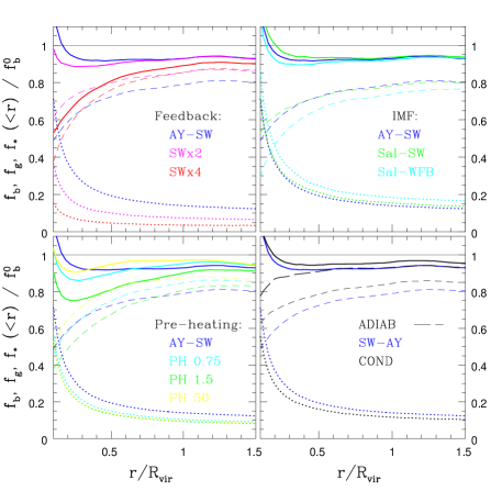
Figure 1: Cumulative mass fractions of the baryon (solid lines), gas (dashed) and stellar (dotted) components of “Virgo” cluster, normalized to the baryon fraction of the cosmic background used (0.12). In the fourth panel the adiabatic curve gives $f_{b}=f_{g}$.

Figure 2: Baryon (thick lines) and gas (thin lines) cumulative mass fractions of groups and “Virgo” simulated with the AY-SW standard scheme, normalized as in previous Fig.

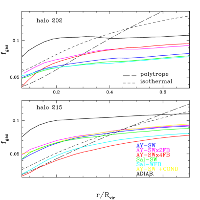
Figure 3: Mass fraction of the ICM gas in the large groups 215 and 202 (all models, solid lines), compared with those derived by Rasmussen & Ponman (2004), assuming either a polytropic or an isothermal temperature profile on two X-ray bright groups of comparable size as our simulated ones (dashed lines): WARPJ0943.5+1640 and WARPJ0943.7+1644.

3.2 Correlations with cluster temperatures

The total baryon fraction distribution is the combined result of the relative contributions given by its gas and stellar components. Evidence for trends in the mean gas fraction with cluster temperature is ambiguous: a decrease in low–T systems would represent a significant contribution to the steepening of the $L_{X}-T$ relation (see Section 6), which could be explained by both lower gas concentration and lower gas fraction (Arnaud & Evrard 1999), especially in models with galactic winds. Several studies have found that the stellar component is predominant in lower-temperature systems, whose lower relative gas content and inflated gas distribution might be consequence of a stronger response to feedback in shallower potential wells (Metzler & Evrard 1994), although probably not at virial sceles: indeed this sequence appears very weak even at $R_{200}$, being more evident only at inner $R_{2000}$, as found by Roussel et al. (2000). Sanderson et al. (2003) have however found a “clear trend” for cooler ($\sim$ 1 keV) virialized systems to have a smaller mass fraction of emitting gas already at $0.3R_{200}$, which gets slightly levelled off when estimated at $R_{200}$ and which is anyway subject to somewhat considerable scatter. In Fig. 4 we actually find a trend in the gas fraction measured at $R_{500}$ with temperature, for the same feedback parameter: in fact the adiabatic curve lies well above the others (because of no star formation) and does not exhibit any systematic trend, whereas an increase is evident in all the AY-SW runs, as well as SWx2 and SWx4 ones. With this regard, the trend we predict is in excellent agreement with the data, although the large scatter of the latter does not allow us to single out a best model among the different physical prescriptions for IMF and feedback.

A constant baryon fraction with size would be consistent with the similarity of $f_{b}$ profiles and an equally constant gas-to-stellar mass ratio (linked to the cold fraction: see Section 7), as found by Roussel et al. (2000), indicating that non-gravitational processes are not dominant in determining the properties of the ICM on large scale (see also White et al. 1993). However both an increase of gas fraction (albeit modest) and $\frac{M_{gas}}{M_{*}}$ with cluster richness have also been separately reported (Arnaud et al. 1992, David et al. 1995), so that the issue is still debatable. From combining the two panels of Fig. 4 it is clear that a trend, if any, would be imputable to the gas component only, given that the stellar fraction follows a fairly constant trend. The $f_{b}$ behaviour confirms that its value is noticeably lowered by galactic feedback by almost one third on average; but above all shows that it is the feedback which is responsible for the increase of about twice in $f_{g}(R_{500})$ going from 1 to 5 keV.

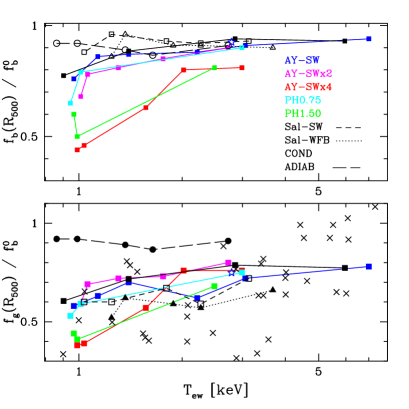
Figure 4: Baryon (upper) and gas (lower) cumulative gas fractions ($f_{b}=f_{g}+f_{*}$) at $R_{500}$, normalized to cosmic $f_{b}$ adopted. Gas data (crosses) from Sanderson et al. (2003).

4 Temperature distribution

Spatially resolved spectroscopical measurements of the ICM temperature provide crucial information on its thermodynamical state: through assuming hydrostatic equilibrium, the total gravitational mass of a cluster is estimable as a function of gas temperature and density profiles. X-ray based determinations of the cluster mass generally assume isothermality for relaxed (non-merging) systems with symmetric morphology, like those in our sample. While to first approximation the ICM appears then to be isothermal, notwithstanding many recent data available from ASCA, XMM, BeppoSAX, Chandra satellites for large samples of rather hot ($T\raisebox{-3.8pt}{$\;\stackrel{{\scriptstyle\textstyle>}}{{\sim}}\;$}4$ keV) systems (Markevitch 1998, Allen et al. 2001, De Grandi & Molendi 2002, Ettori et al. 2002, etc.) agree on presenting declining temperature profiles in the outer regions at $r\raisebox{-3.8pt}{$\;\stackrel{{\scriptstyle\textstyle>}}{{\sim}}\;$}0.2-0.3R_{vir}$, displaying a “universal” shape featuring as $T\propto[1+(\frac{r}{R_{c}})^{2}]^{-\frac{3}{2}\beta(\gamma-1)}$, with $\beta\simeq\frac{2}{3}$, $\gamma\simeq 1.2-1.3$. Such a decline implies that the assumption of hydrostatic equilibrium along with isothermal $\beta$-model of gas density distribution lead to underestimate the gravitating cluster mass enclosed within small radii, whilst overestimating it at large distances. In addition, for most clusters hosting cooling flows a fair temperature descent was reported towards the centre, after a peak at around $0.1R_{vir}$, which reveals the presence of a cooling or cold innermost centre surrounded by a somewhat extended isothermal core: this feature seems to be reproduced by adiabatic simulations in the literature (Borgani et al. 2001, Valdarnini 2003), but it vanishes as soon as cooling is introduced, giving rise to an increasing temperature profile almost to the centre. It has been proposed (Voigt et al. 2002) that thermal conduction, besides conventional heating, could help regulating central gas cooling: heat would be transferred from the outer layers to the centre, allowing diffuse gas to be kept at fairly low temperature ($\sim$ 1 keV) without cooling out. However, observations of cold fronts in many clusters indicate that thermal conduction is significantly suppressed in the ICM.

In Fig. 5 we compare temperature profiles derived from our simulated “Virgo” with the results by De Grandi & Molendi (2002), who analysed spatially resolved data for a sample of rich nearby clusters with BeppoSAX, both cold–core and non cold–core by about the same proportions, finding that their profiles are characterized by a drop in temperature inside of 0.1$R_{vir}$: beyond this they steeply decline outwards following a power-law, which is flatter for the cold–core systems; more specifically, the polytropic indices of the power-law decline are closer to the isothermal value $\gamma=1$ for cold–core clusters and to the adiabatic value $\gamma=\frac{5}{3}$ in clusters without a cold core: the latter are in fact supposed to have undergone more recent major mergers, so that they have not had time enough for heat transport to efficiently flatten their temperature profiles. Such results for cold–core clusters are also confirmed by Piffaretti et al. (2005), who give temperature and entropy profiles of 13 nearby clusters with cooling flows.

In the four panels the separate role of feedback, IMF, pre–heating and conduction may be assessed by varying the relevant parameters and keeping the SW scheme with AY IMF as standard reference for all. The most striking pattern is given by the two extreme runs SWx4 and the weak feedback one, which are the only ones resulting in an unrealistic temperature spike at the centre. As one can notice in Fig. 6, these are also the (only) runs displaying a significant high level (“floor”) of central entropy, almost an order of magnitude higher with respect to others, meaning that they must have a central gas density almost 20 times lower, since $S\propto T/n_{e}^{2/3}$. As a consequence, at the same radial distance their gas has a long cooling time, preventing the onset of cooling flows. The reasons for this peculiar central behaviour root in the structural preparation of these simulations: the WFB simulation, in which gas gets rapidly cooler out of $\sim 0.1R_{vir}$, adopts an almost primordial cooling function due to the very low metallicity in the ICM, so that cooling is far less efficient than for the other runs even in systems larger than groups; on the other hand the weak propagation of stellar feedback from the inner sites of star formation causes the gas to get settled at the centre. On the contary, the strongest super–wind scheme ends up with more violently spreading the gas out to larger radii and thus rarefying the inner density.

With the exception of the Sal-WFB case, all the runs fairly well reproduce the observed decline from $\sim 0.25R_{vir}$ outwards. The introduction of strong feedback and/or preheating smooths out the sharp central temperature peak of the WFB case (typical also of simulations with only cooling and star formation) so that the profiles remind more closely the observational shape; however, the formation of an isothermal core around $0.1R_{vir}$ is not satisfactorily modelled by any of the simulations: temperatures keep rising inwards even beyond $0.1R_{vir}$ and the turn–over occurs only at around $0.05R_{vir}$. Further increasing the feedback strength does not cure the problem, as clearly indicated by the behaviour of the SWx4 run discussed above (first panel).

In the third panel, preheated runs are compared with the standard AY-SW and with the adiabatic one: the effect of early injecting 0.75/1.50 keV or 50 keV$\cdot$cm² per particle are practically equivalent. Both the standard and the preheated runs are clearly less flat than the gravitational-only one at outer distances from $\simeq 0.25R_{vir}$, while the latter is steeper at the core scale.

As for thermal conduction, its main effect is to flatten the profile at large radii, showing that for conductivities of 1/3 the Spitzer value, this mechanism can even temperature gradients out on large scales. In particular, for “Virgo” conduction does somewhat smooth the temperature profile around 0.1 $R_{vir}$, but by far not enough to reconcile it with the observational profiles. The “Coma” simulation discloses instead an interesting feature: the erratic behaviour of the temperature curve around the core, which by direct inspection of the simulated cluster is recognized as due to cold fronts, is completely smoothed out by conduction. Since cold fronts are observed in many clusters, this indicates that thermal conduction is highly suppressed in the ICM, presumably by magnetic fields.

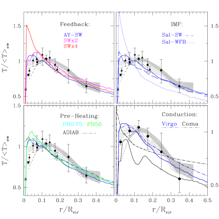
Figure 5: Temperature radial profiles of “Virgo”, normalized to their mean emission-weighted temperature; all panels present AY-SW as reference. At bottom right also shown “Coma”. Data points from De Grandi & Molendi (2002) give the average deprojected profile over a sample of nearby clusters, both CF (dash-shadowed) and non-CF (point-shadowed); also shown some individual CF clusters: A1795 ($<kT>=6.10$ keV, circles), 2A0335 (3.38 keV, squares) and Centaurus (3.77 keV, triangles).

5 Entropy

The dynamic and X-ray properties of the ICM of relaxed clusters are on large scale determined by the entropy distribution of the inter-galactic gas adjusting itself to fit into the dark matter potential well it lies within. The intra-cluster gas entropy (defined as $S=kT/n_{e}^{2/3}$, a quantity conserved in adiabatic processes) gravitationally generated across the growth process of cosmic structure changes its distribution by means of radiative cooling and non-gravitational heating, and in turn determines gas properties such as density and temperature profiles (Voit et al. 2002; Borgani et al. 2001).

Observations of X-ray surface brightness profiles in inner regions of poor clusters and groups ($T\raisebox{-3.8pt}{$\;\stackrel{{\scriptstyle\textstyle<}}{{\sim}}\;$}2$ keV) had pointed towards the existence of an “entropy floor” in the ICM/IGM at around 100 keV$\cdot$cm² (Ponman et al. , 1999, Finoguenov et al. 2002), breaking the self-similarity of group and cluster ICM profiles. Systems at all scales, and in particular low-mass ones, show evidence for excess entropy compared to that expected from pure gravitational entropy increase by shocks (see Introduction).

In our approach we also included a set of simulations with additional preheating, basically following Borgani et al. (2001, 2002) in setting an entropy floor through early instantaneous preheating of 0.75-1.50 keV or 50 keV$\cdot$cm² per particle at $z=3$, which is the epoch at which heating sources are expected to contribute significantly (close to peak of star formation in proto-clusters). An impulsive energy/entropy budget of the order we used is motivated by X–ray phenomenology of ICM, and appears also consistent with detected abundances (see Tornatore et al. 2003).

However, observations of groups have recently hinted towards a lack of large isentropic cores, at variance with predictions of preheating models (Ponman et al. 2003). Especially massive virialized systems with strong cooling flows do not show such cores, rather a monotonically increasing entropy with radius (Piffaretti et al. 2005 and references therein). On the other hand, high entropy excesses have been reported up to large radii even in moderately rich clusters (Finoguenov et al. 2002). In fact, whilst the existence of isentropic cores is still controversial, both analytical estimates of the effect of shock heating on the preheated accreting gas (Tozzi & Norman 2001) and numerical simulations (Borgani et al. 2001) indicate entropy profiles outside the cluster’s central region having a slope $S\propto r^{1.1}$, or closely shallower.

Another explanation could appeal to cooling alone as able to remove low-entropy gas from the haloes’ centre, but this class of models inevitably leads to overcooling (Knight & Ponman 1997, Davé et al. 2002). It is clear that the most natural and comprehensive way to model the inner distribution of entropy, as well as the X-ray emission, is to accompany cooling with heating by feedback subsequent to star formation: this will heat gas particles at low entropy. The entropy threshold in the core would be then set up by equating the gas cooling time to a Hubble time, such that the floor itself will scale as $S_{f}\propto(\tau_{cool}T)^{2/3}$ and will be higher in hotter systems, as to reproduce the observed smooth flat trend with temperature (Voit & Bryan, 2001).

In Fig. 6 the inner pattern of temperature and entropy for particles in the “Virgo” cluster is shown in more detail, from which it is evident that there is not a proper isentropic core or entropy floor: most models exhibit central entropy values of $\sim 10-20$ keV$\cdot$cm², in agreement with inferred values for cold–core clusters (Voit et al. 2003); instead a plateau around 100 keV$\cdot$cm² has formed only in two distinct cases, namely the WFB scheme with Salpeter IMF and the 4-times SW scheme with AY IMF. The former has less efficient cooling and therefore does not develop a low-entropy core; at the same time, the higher star formation rate (because less hampered by weaker feedback) also contributes to absorb larger amounts of low–entropy gas. The SWx4 model ends up with forming a floor around 100 keV$\cdot$cm² at $z=0$, much higher than the entropy level reached by the preheated runs; preheating indeed seems to have a minor impact on the behaviour of the standard SW simulations. The adiabatic run also develops an entropy floor of about 30 keV$\cdot$cm², but only at the very centre ($r\leq 0.01R_{vir}$), where gas keeps accumulating without cooling.

The entropy floor is even more evident in our simulations of groups (Fig. 7), where not only the aforementioned WFB and SWx4, but also the preheated runs, exhibit evidence for an isentropic core at $\sim$ 100-250 keV$\cdot$cm² up to $\sim 0.3R_{vir}$; while the adiabatic one clearly lies the lowest (except that at the innermost $\sim 0.05R_{vir}$) and all other profiles fall in between, following a smooth coreless increase from the centre. In this way, coupling cooling and star formation with feedback allows one to reproduce the entropy excess observed at least at groups scale: namely, cooling and star formation alone make low-entropy gas particles be selectively removed from the diffuse hot phase in central regions, hence leaving a flatter profile. Imposing then an artificial entropy floor at high redshift onto this has a slight effect on increasing the gas cooling time and thus slowing down star formation, so that the final entropy level gets lower due to less efficient cooling. When properly incorporating energy and metal feedback from star formation, one can see how the gas entropy actually ends up at a lower level.

In order to highlight the effects of non-gravitational physics on the gas radial distributions, we show in Fig. 8 the scaled entropy $S/T$ for two groups, whose characteristics are comparable to those of the X-ray bright galaxy groups studied by Rasmussen & Ponman (2004). Indeed self-similar scaling with mass would lead to the relation $S(r)\propto T$ and spherical shock heating models as well as simulations predict the power law $S(r)\propto r^{1.1}$, which is also plotted for comparison. In general all our simulated profiles get steeper than this when approaching the virial radius, whilst they flatten inside $\sim 0.1R_{vir}$ as a result of a core in the density distribution. The mean slope outwards $0.1R_{vir}$ appears however to follow that for clusters (see Piffaretti et al. 2005). The only evident entropy core has formed again in the SWx4 simulation and in any case no core at all can be seen extending beyond this rather small radius: this is consistent with some recent observations of groups (e. g. Pratt & Arnaud, 2003), which do not detect in poor systems the large isentropic cores predicted by simple preheating models.

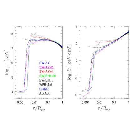
Figure 6: Temperature (left) and Entropy (right) profiles of “Virgo”, all models.

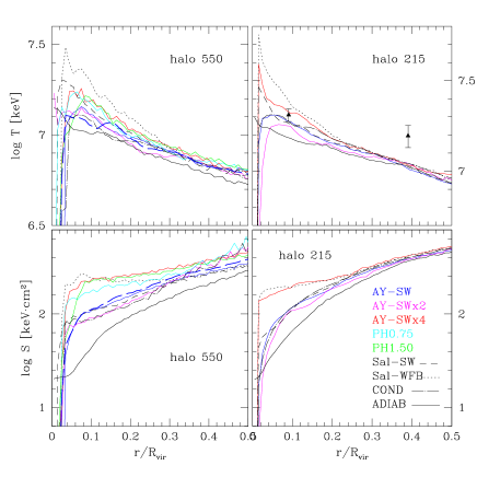
Figure 7: Temperature (top) and Entropy (bottom) profiles of the groups 550 and 215 (all models) at $z$=0. Also shown temperature profile of group 550 at high (8x) resolution (thick long-dashed lines). T-data points from Rasmussen & Ponman, 2004.

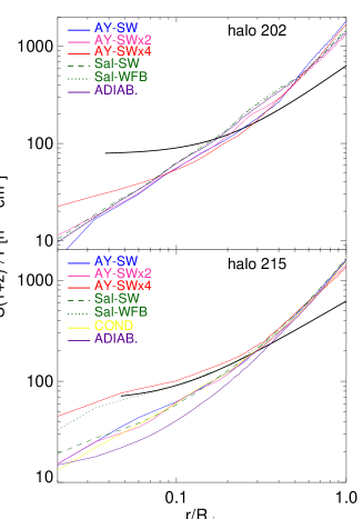
Figure 8: Scaled entropy as a function of radius. Dot-dashed: normalized self-similar profile $S\propto r^{1.1}$ expected from pure gravitational shock-heated spherical accretion. Thick lines: scaled entropy in the two bright groups of Rasmussen & Ponman (2004), obtained by assuming polytropic gas temperature profiles.

6 X-ray Luminosity

The relationship between bolometric luminosity and temperature provides a sensitive diagnostics of the gas to virial mass ratio and an indication as well of the lack of self–similarity in the structure of clusters.

Measurements of ICM temperature by X-ray satellites demonstrate that the observed systems scatter around the curve $L_{X}\propto T^{\alpha}$ with $\alpha\simeq 3$ for clusters at $T\raisebox{-3.8pt}{$\;\stackrel{{\scriptstyle\textstyle>}}{{\sim}}\;$}2$ keV (Mushotzky 1984, Edge & Stewart 1991, David et al. 1993, Markevitch 1998, Arnaud & Evrard 1999, Ettori et al. 2002), approaching to the self-similar scaling only from $T\raisebox{-3.8pt}{$\;\stackrel{{\scriptstyle\textstyle>}}{{\sim}}\;$}8$ keV on. The relation itself has been found fairly constant over redshift up to $z\sim 1$ (see Donahue et al. 1999, Borgani et al. 2001). The largest deviations from it are found for those systems whose emission is strongly associated with a cold core, or “cooling–flow” (Fabian 1994), whose effect has to be corrected for (Markevitch 1998, Allen & Fabian 1998, Arnaud & Evrard 1999, Ettori et al. 2002). This class of clusters represents slightly more than half of all nearby X-ray detected clusters. Moreover there is evidence that low-mass systems ($T\raisebox{-3.8pt}{$\;\stackrel{{\scriptstyle\textstyle<}}{{\sim}}\;$}1$ keV) show a steeper relation, up to $L_{X}\propto T^{8}$ (Ponman et al. 1996, Helsdon & Ponman 2000b).

As sketched in the Introduction, this discrepancy with gravitational-only (non-radiative, or “adiabatic”) hierarchical models of spherical accretion indicates a segregation of dark and gaseous matter. Pre–heating of the ICM later followed by merger shocks could steepen the $L_{X}-T$ dependence of cooler clusters (Cavaliere et al. 1997) and at the same time decrease the luminosity evolution to redshifts $z\sim 1$, as observed. When cooling and star formation were included in the simulations, the resulting emission profiles got flatter at the core due to gas removal from the hotter phase, while incorporating also additional heating on this has produced spikes in the inner X-ray luminosity density if the epoch of pre–heating was as early as $z=9$ (Borgani et al. 2001). Tornatore et al. (2003) have found that cooling plus star formation only are able to fairly suppress the X-ray luminosity, but at the same time are responsible for steepening the temperature profiles, leading to an increase in the emission–weighted temperature; the net effect is to enable a match between simulated and observed clusters in the $L_{X}-T$ plane, though not at group scales. Including later ($z=3$) pre–heating mainly affects small systems, further suppressing their emissivity, so that altogether the combined effect of cooling and pre–heating is for simulations to approach the slope of the observed $L_{X}-T$ relation.

Besides cooling, star formation and energy feedback, our procedure included as well a self–consistent treatment of the metal enrichment of the ICM regulated by the stellar feedback itself, in such a way that it is possible to estimate also the contribution heavy elements make to the emissivity. In general each gas particle has an assigned mass, density (hence a volume $\Delta V_{i}$), temperature, metallicity $Z_{i}$ and energy, so that its bolometric luminosity at X-ray band can be computed as

$$L_{X}=\sum_{i}L_{X}^{i}=\sum_{i}\Lambda(T_{i})_{Z_{i}}\cdot n^{2}_{H_{i}}\cdot\Delta V_{i}$$ (2)

where $\Lambda$ is the metal-dependent cooling function such that the emissivity reads $\epsilon=\Lambda(T,Z)\cdot n_{H}^{2}$, and which scales as $\Lambda(T,Z)\propto\sqrt{T}$ for $T\gg 10^{6}$K. The contribution of metal lines to global emissivity, which is dominated by Bremsstrahlung from a primordial-like gas, gets even more relevant at group scales, where it can make up to half of the total. From this, the emission-weighted temperature is obtained as

$$\langle T\rangle=\frac{\sum_{i}L_{X}^{i}\cdot T_{i}}{\sum_{i}L_{X}^{i}}$$ (3)

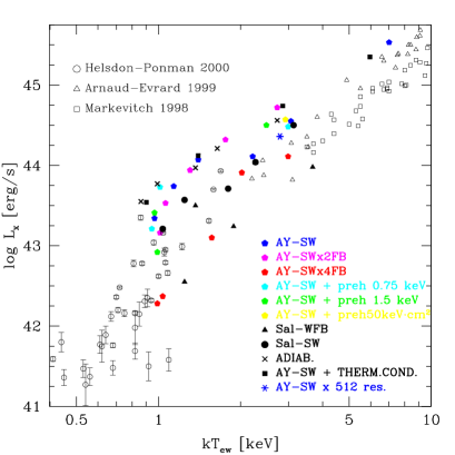
Figure 9: X-ray luminosity - emission weighted temperature scaling relation from the inner 1 Mpc. Simulated points are the average over the last ten frames down to z=0. High-resolution Virgo shown at $z=0.1$. Open symbols are X-ray data from Markevitch (1998), Arnaud & Evrard (1999), Helsdon & Ponman (2000a).

In Fig. 9 the X-ray luminosity–(emission-weighted) temperature relation for all our simulations at $z\simeq 0$ is shown, along with observations. The observed (open) points exhibit the characteristic double-slope behaviour; as expected, the adiabatic runs lie above this curve, but interestingly adding thermal conduction results in a similar overestimate of the X-ray emission as well. Overall, the predicted luminosities are higher than the observed ones; both enhanced feedback and a less top–heavy IMF, however, can lower the X-ray luminosity: the latter effect seems to be dominant, since the runs with Salpeter IMF and Weak Feedback, which result in a low level of metal enrichment as well (see next sections), are those placed lowest. All in all, when strengthening the feedback up to 4 times and using a top–heavy IMF, a satisfactory level seems to be reached at least for clusters, whereas it results in a too drastic suppression of the X-ray luminosity for the lower mass haloes, though matching the slope of the $L_{X}-T$ relation. A preliminary conclusion from these results could be that the success of previous generations of simulations in reproducing both the L-T relation, the surface brightness profiles and the rather high entropy floor, may have been somewhat favoured by the simplistic use of primordial or uniform cooling functions; when making the models more realistic by including chemical evolution and metal-dependent radiative cooling, this promotes the development of fairly strong central cooling flows, which generally lead to excess X-ray luminosities.

Finally, in Fig. 10, we show the effect of the numerical resolution on the computation of the luminosity, in the case of “Virgo”: as it can be noticed, increasing mass resolution by 8 times and force resolution by twice, affects only slightly the global X-ray luminosity, the largest contribution to which being that of the innermost denser region, which is now better resolved.

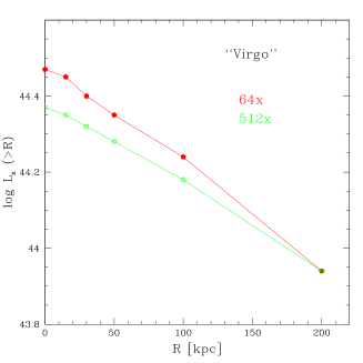
Figure 10: X-ray luminosity emitted from the gas contained between $R$ and $R_{vir}$, for “Virgo” run at normal (red, pentagons) and high (green, stars) mass resolution, both at $z=0.1$.

6.1 X-ray luminosity and star formation evolution

Besides the ICM, star forming galaxies too are known sources of X-ray emission, which can be considered as a tracer of the most energetic phenomena associated with phases of star formation and evolution, such as mass accretion, SN explosions and remnants, hot stellar winds and galactic outflows. While point sources (X-ray binaries, SN remnants) account for the dominant contribution to the overall X-ray emission in the 2-10 keV band, where they give the spectrum a power–law shape, diffuse emission (the thermal component) is significant in the soft X-ray band, arising from the ISM shock heated by supernovæ in the form of shells or winds (Persic & Rephaeli 2002). Moreover, AGN X-ray emission correlates with enhanced star formation (starburst) sites: the X-ray emissivity normally overwhelms that from the host galaxy itself.

A relationship between far-infrared (FIR) and X-ray luminosities in star forming galaxies has often been found in both soft and harder X-ray bands (e. g. David et al. 1992; Lou & Bian 2005 from ROSAT in the soft 0.1-2.4 keV band; Ranalli et al. 2003 from ASCA, Bepposax and Chandra in the hard band; Franceschini et al. 2003 from XMM in the hard 2-10 keV band): since radio and FIR luminosities are well known indicators of star formation, it follows that $L_{X}$ at both 0.5-2 keV and 2-10 keV should as well provide an estimate of the star formation rate (SFR). Besides, spiral galaxies in the field or cluster outskirts may still be embedded in extended reservoirs of hot emitting gas still accreting onto their discs. The gas accretion history of the disc is thus indirectly reflected by the galaxy X-ray luminosity: the hot gas infalling from the halo cools out with a mass cool-out rate inversely proportional to its cooling time and following Rasmussen et al. (2004) it approximately scales with the bolometric luminosity and the emission-weighted mean inverse temperature: $\dot{M}\propto L_{X}\langle\frac{1}{T}\rangle_{ew}$.

In Fig. 11 we check for the same relationship in tracing the redshift evolution of the predicted gas cool-out rate and global star formation rate of the whole cluster for the two largest simulated systems: it is noticeable that the two quantities are well correlated, although the predicted cool-out rate is systematically higher by a factor $\sim$3. The offset between the two quantities is due to: a) the simplistic assumption behind the equation we took from Rasmussen et al. (2004), where $PdV$ work was neglected; and b) the fact that, given the strong galactic super-winds, not all gas which cools out is turned into stars.

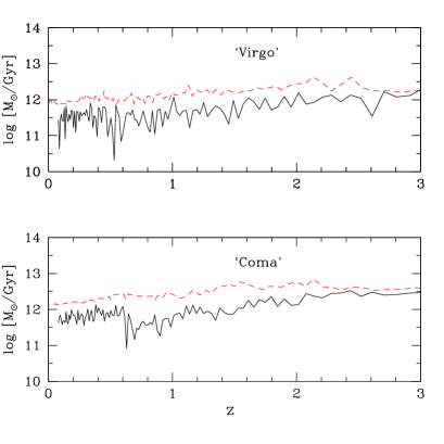
Figure 11: Star formation rate (solid) in “Virgo” (AY-SW) and “Coma”, including the cD and all the stars (both inter- and intra-galactic), compared with the mass cool-out rate $L_{x}\langle\frac{1}{T}\rangle_{ew}$ by X-ray emission (dashed) as predicted by simple model in Rasmussen et al., 2004.

7 The cluster cold components

The baryonic mass of clusters is largely dominated by the hot ICM mass, yet the mass fraction of the cold component (which is the sum of stars and, although to a much smaller extent, the neutral, non X-ray emitting gas phase at $T\mathrel{\hbox to0.0pt{\lower 3.0pt\hbox{$\sim$}\hss}\raise 2.0pt\hbox{$<$}}10^{4}K$) is a crucial constraint for cluster simulations, as it plays a major role in distinguishing the mechanisms responsible for the “excess entropy”: the larger the cold fraction, the larger the contribution given by star formation in removing low entropy gas from the ICM. To match the observed cold fraction of $f_{c}=0.1-0.2$ (see below), strong (pre)heating or feedback are needed to enhance the entropy level (see Section 3.4). Also, the cold fraction constrains the chemical enrichment efficiency of the stellar populations — which are evidently able to enrich to significant levels the hot ICM gas mass $M_{ICM}>>M_{*}$ (Section 8). The cold fraction, defined as the fraction of baryons in the form of cold gas and stars, provides a measure of galaxy formation efficiency and can be recast in terms of the gas and stellar mass-to-light ratios (MLR) as

$$f_{c}^{-1}\simeq 1+\frac{M_{ICM}}{L_{B}}\left(\frac{M_{*}}{L_{B}}\right)^{-1}$$ (4)

Its empirical estimate however is non–trivial: while the ICM gas mass is determined fairly directly from X-ray data, the stellar mass $M_{*}$ can be derived only indirectly from the observed luminosity of cluster galaxies, typically in the B band, and is subject to uncertain assumptions on the stellar mass-to-light ratio; the latter likely spans the range 4-8 $\frac{M_{\odot}}{L_{\odot}}$, according to the IMF (Portinari et al. 2004). Thus, with the ratio $\frac{M_{ICM}}{L_{B}}$ directly observable and typically $\simeq 30h^{-\frac{1}{2}}\frac{M_{\odot}}{L_{\odot}}$ (Moretti et al. 2003; Finoguenov et al. 2003) , the corresponding cold fraction $f_{c}\simeq 10-20\%$ has a factor-of-two uncertainty stemming from the assumed stellar MLR (see Portinari 2005 for a detailed discussion). Due to the importance of this constraint on cluster physics, care should be taken in comparing simulations and observational estimates consistently (i.e. assuming a coherent stellar MLR), especially since the Salpeter and AY IMFs of our simulations are quite “heavy”, i.e. with a significant stellar mass locked in low–mass stars and remnants (Portinari 2005). The corrections can be sometimes quite significant (e.g. in Fig. 13).

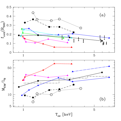
Figure 12: (a) Cold fraction at $R_{500}$ and $z$=0. “Virgo” is shown at both normal and high resolution: the latter (at $z=0.1$) with (star, since $z=2$) and without (open star) cooling flow correction. Data in the K-band from Lin et al. 2003 are provided with an upward arrow indicating a 30% (20%) shift to consistently match the simulations with Salpeter (AY) IMF (see text). (b) Mass-to-light ratio of the hot ICM gas in the B-band. Luminosities have been calculated from all the stars formed within $R_{500}$: for “Virgo” and “Coma” is also shown (dot-longdashed) the effect of dropping the young stars at the very centre of the cD (see text). Data from Finoguenov et al. 2003 (dot-dashed: average over cluster samples). Colours as in Fig. 4 and 18.

In Fig. 12a, the cold fractions of our simulations are compared to the recent data by Lin et al. (2003; hereinafter LMS) who accurately derive stellar masses from K–band luminosity (a better mass tracer than B band), distinguishing between spirals and ellipticals in assigning the MLR. Yet the zero–point of the absolute value for the stellar MLR depends on the assumed IMF; the MLRs adopted by LMS (from Bell & de Jong 2001 for spirals and Gerhard et al. 2001 for ellipticals) are about 30 (20)% smaller than those of the Salpeter (AY) IMF. This implies that, by assuming a Salpeter (AY) IMF consistent with our simulations, the underlying stellar mass and the cold fraction would be 30 (20)% larger than inferred by LMS; these corrections are shown as vertical shifts in Fig. 12, nonetheless they are by far not yet sufficient to bring the Salpeter simulations in agreement with the data; especially those with weak feedback predict too large $f_{c}$.

Good agreement with the data is obtained instead for the “standard” AY-SW simulations, with or without pre-heating and conduction. In Fig. 12a we show the cold fraction of the high resolution “Virgo” simulation (quite close to the normal resolution one), along with the one corrected for the mass of the central cooling flow stars (Section 2.2): neglecting the latter population reduces $f_{c}$ by about 20%. As to the simulations with enhanced feedback efficiency, the SWx2 simulations are still in reasonable agreement with the observations, while the extreme case SWx4 yields too low cold fractions for $T>2$keV, where data are available.

Alternatively, rather than correcting the observational cold fraction consistently with the specific IMF and MLR pertaining to each simulation, we can compute the stellar luminosity of our clusters and compare to the directly observed $\frac{M_{ICM}}{L}$ ratio. The global luminosity within $R_{500}$ is the sum of the luminosities of all the star particles, each computed from SSPs with the corresponding age, metallicity and IMF (see Paper II for details). Again, when computing the cluster luminosity, we neglect the artificial late stellar populations arisen from innermost cooled region (see Section 2.2), in the same way as for the “Virgo” cold fraction above.

In Fig. 12b we plot the ICM MLR from our simulations, compared to the B-band data of Finoguenov et al. (2003), for volumes within 0.4 $R_{vir}$. In agreement with the top panel, the AY-SW simulations best reproduce $\frac{M_{ICM}}{L_{B}}$ and hence the cold fractions; also the trend with temperature is well modelled. For the extreme feedback case AY-SWx4, the low cold fractions on top corresponds as expected to high $\frac{M_{ICM}}{L_{B}}$. For the Salpeter simulations, also consistently with the too large cold fractions found above, the luminosity is too large for the corresponding ICM mass and $\frac{M_{ICM}}{L_{B}}$ is too low; the excess luminosity is even more striking in B band, because in the Salpeter simulations the galaxies are more metal poor and hence bluer, than real cluster galaxies (see the colour-magnitude relation in Paper II).

A number of studies suggest that the cold fraction decreases at increasing cluster mass or X-ray temperature (David et al. 1990; Arnaud et al. 1992; LMS) — though the issue is still debated, and it might depend on the sampled volume in different clusters (Roussel et al. 2000). The trend is usually explained by invoking less efficient star and galaxy formation in hotter systems; indeed LMS have recently found that the stellar mass fraction over the total cluster mass, decreases for more massive clusters. To this regard, an important role is also played by metal dependent cooling, especially when coupled with efficient mechanisms of transportation and mixing of the heavy elements into diffuse gas at outer radii, which has yet to cool out (Scannapieco et al. ., 2005): thus, in more massive haloes the effects from non-primordial cooling function (as that we use, except in the WFB model) are possibly counteracted by chemical mixing occurring at larger scale. Another factor contributing to the trend is the likely gas dispersal out of the shallower potential wells of smaller systems, reducing their ICM mass and overall baryon fraction.

For our simulated sample as well, the cold fraction decreases with increasing mass (Fig. 12a). The trend is driven by the fact that larger clusters better retain the ICM gas, so that the ICM to total mass ratio increases, while the stellar mass fraction remains fairly constant with cluster temperature (cf. Fig. 2 and 4). The latter behaviour is in conflict with observations; notice, however, that the observed stellar mass fraction typically refers to the stars in galaxies: the intra-cluster population is not taken into account here and it might compensate for the observed descrease, if the percentage of intra-cluster stars increases with cluster mass, due to more efficient stripping (LMS; see Paper III).

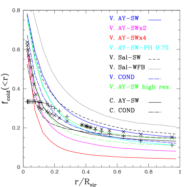
Figure 13: Cold gas plus stellar radial profiles of the two clusters. Also shown “Virgo” at higher resolution (thin lines), both with (long-dashed) and without (solid) cooling flow correction since $z$=2. The observed cold fractions derived from $\frac{M_{*}}{M_{ICM}}$ of Roussel et al. (2000) are overplotted (+ for King light profiles, $\times$ for de Vaucouleur’s).

Non-gravitational heating mechanisms (SN/AGN-driven galactic winds; pre-heating) also affect the radial profiles of the cold fractions. In Fig. 13 we compare our two largest simulated clusters to the observed profiles of Roussel et al. (2000); the + and $\times$ symbols correspond to the results they obtain fitting King or de Vaucouleur light profiles, respectively; the latter are better comparable to our simulated clusters where the light is centrally peaked due to the cD’s. Once more the AY-SW simulations (including the conduction and preheating cases) are those that best reproduce the overall cold fraction within $R_{500}$. Again, as previously in Fig. 12, the effect on the cold fraction of removing stars belonging to the base of the cooling flow is highlighted: in particular the high resolution and corrected “Virgo” simulation (dashed green line) turns out to be in very close agreement with observed profiles.

All in all, it is a positive result that our simulations with supernova feedback (with a top-heavy IMF, but without other energy sources such as AGNs) fairly reproduce the observed low cold fractions. Previous simulations including radiative cooling and star formation typically predicted too large a fraction of gas converted into stars, with SPH as well as with Adaptive Mesh Refinement schemes (Tornatore et al. 2003 and references therein; Kravtsov, Nagai & Vikhlinin 2005). When artificial pre-heating is also invoked, star formation is hampered at high redshift, which helps to reduce the cold fraction but also causes an unrealistic delay in the star formation history (Paper II; Tornatore et al. 2003; Nagai & Kravtsov 2004). Dumping the supernova energy just as thermal energy in the surrounding gas has little effect on the cold fraction (Tornatore et al. 2003; Nagai & Kravtsov 2004); hence the key to our result is a feedback implementation able to represent more realistically the adiabatic phase of super-shell expansion.

8 Metal enrichment

The hot ICM gas in clusters is significantly enriched in metals. In our simulations, the super–winds resulting from SNII enrich the ICM by dispersal of the chemical elements produced by stars (Section 2.3 and  2.1). In this scheme, the dispersal of SNII products is favoured; however, metals ejected by lower mass stars and SNIa are blown out as well (and are important for the ICM enrichment), because the super-winds also expel gas already present in the galaxies.

As to the role of ram pressure stripping, though in principle included in the hydrodynamical simulations, it is here only partially resolved: stripping of hot and diffuse galaxy halo gas is resolved, whilst stripping of high density, cold (HI) gas in the galaxy itself is not. There are however arguments that ram pressure stripping is not the dominant mechanism of extraction of metals from galaxies (Renzini 1997; Aguirre et al. 2001, but see also Domainko et al. 2006 and Section 8.4).

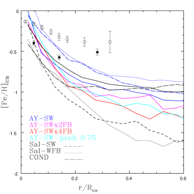
Figure 14: Iron gradients at $z$=0 in the ICM of the two simulated clusters (same symbols as previous figure: “Virgo” at higher resolution as thinner solid line). Data from De Grandi et al. (2004) refer to coldcore (open circles) and non-cold core (filled squares) clusters.

8.1 The iron content of the simulated clusters

In rich clusters the iron abundance is about one third of the solar value, with a rather small dispersion (Arnaud et al. 1992; Renzini 1997; Fukazawa et al. 1998; Baumgartner et al. 2005); detailed iron profiles suggest though that cool core (formerly called cooling flow) clusters have systematically higher ICM metallicities (De Grandi et al. 2004, hereinafter DELM; Fig. 14). The iron abundance profiles show negative gradients: cool–core clusters display a central peak (up to 0.7 solar), while out of the cool core, as well as in non–cool core clusters, the gradients are much milder and consistent with a flat distribution (DELM).

Fig. 14 compares the iron abundance profiles in the ICM from our simulations, to the data for cool core and non-cool core clusters; the former are a better reference for our simulated clusters, which are well relaxed objects with prominent central cDs. Evidently, our profiles are steeper than the observed ones — a general problem in simulations (Tornatore et al. 2004), partly related to the fact that star formation at late times is concentrated toward the central regions.

In Fig. 14, the iron abundances of the Salpeter simulations lie well below the observed ones, at all radii; while the standard AY-SW simulations are closer to the data. However, since the distribution of the metals is different between simulations and real clusters, quantitative comparison of the level of chemical enrichment can be made considering the global metal content of the ICM only.

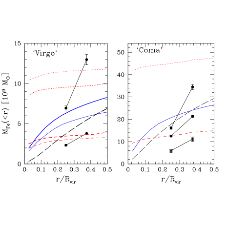
Figure 15: Cumulative Iron mass distributed in stars (red, dotted: uncorrected; dashed: corrected for the cooling flow stars since $z=2$) and in the ICM (blue, solid), for the “Virgo” (thin line at normal and thick at high resolution) and “mini-Coma” AY-SW simulations. Long-dashed is $M_{Fe}^{ICM}$ assuming $\frac{1}{3}$ solar abundance in the ICM (the two for “Virgo” at different resolutions overlap into the same one). Data points for ICM Fe mass from De Grandi et al. (2004): cold-core (circles) and non cold-core (crosses) clusters of size comparable to the simulated ones: A3526 and 2A0335 Virgo-like; A119 (the only non–cold-core), A426 and A1795 Coma-like.

We consider the AY-SW simulations of the two richest clusters in our set, “Virgo” (at normal and high resolution) and “Mini-Coma”. In Fig. 15 we show as solid lines the cumulative iron mass in the ICM within radius $R$, out to $R_{500}$ (which is $\simeq 0.5R_{vir}$). The dashed lines are the expected cumulative profiles assuming for our ICM gas the typical average iron abundance of 0.3 solar (e.g. DELM). Also plotted are the cumulative iron masses within $R_{2500}$ and $R_{1000}$ determined by DELM for individual clusters with emission–weighted temperatures close to those of our simulated “Virgo” and “Coma”, scaled by a factor $\left(\frac{70}{50}\right)^{-\frac{5}{2}}$ consistent with the $H_{0}$ value we adopt. There is quite some scatter in the actual iron masses of individual clusters, but they nicely bracket the simulation results – especially considering the cool core clusters (filled circles). Out to $R_{500}$, the simulations reproduce the expected values (solid vs. dashed lines) fairly well. We note that if the ICM maintains the typical iron abundance of $0.3\,Z_{Fe,\odot}$ beyond $R_{500}$, then the simulation tend to fall short of the expected metal content of the ICM; however, the observed metallicity profiles typically reach less than $R_{500}$ (e.g. Fig. 14) so that some extrapolation is already involved in Fig. 15.

Observationally the “partition” of the iron mass is skewed in favour of the ICM (Renzini et al. 1993; Renzini 1997, 2004); for the AY IMF in particular, the expected partition is about twice more iron in the ICM than in stars (Portinari 2005). In Fig. 15 instead, the partition is skewed in favour of the stars (solid vs. dotted lines), so that only about 1/3 of the total iron content remains in the ICM. The discrepancy may be partly due to the fact that we compute the iron mass from all the star particles (including the cD, its envelope and the intracluster stars), while observational estimates are based only on galaxies. In very relaxed clusters similar to our simulated ones, the amount of iron contained in the envelope of the cD can be significant; if observationally this is not accounted for, one underestimates the actual star–to–ICM iron mass ratio.

However we find that most of the discrepancy is just an artifact due to significant production and lock-up of iron by stars formed at the base of late time cooling flows: subtracting the iron content from these stars from the cumulative stellar iron mass results in the short-dashed line of Fig. 15. The mass of the stars involved in the correction is only about 20% (e.g. Fig. 12, solid vs. open star) but the effects on the locked up iron mass are major: after the correction, the iron mass partition becomes about 2/3 in the ICM to 1/3 in the stars, in much better agreement with the expectations. As the prominent cooling flow stellar population is a non-physical effect (Section 2.2), the corrected iron masses are to be regarded as much more realistic than the uncorrected ones. This highlights that a proper modelling of the metal partition and of the ICM enrichment is strictly related on improved understanding of the physics of the central regions.

In Fig. 16 we plot the star–to–ICM iron mass ratio for different runs of the “Virgo” cluster, with different physical prescriptions, to analyse the effects of the different IMFs and feedback schemes on the iron partition. Within $R_{500}$ there is typically 2–3 times more iron locked in the stars than in the ICM, i.e. the partition is “inverted” with respect to the expected one as we have seen above. However, besides the cooling flow corrected Virgo simulations discussed above (dashed lines), also the AY-SWx2 or AY-SWx4 simulations (with no correction) result in reasonable star–to–ICM iron mass ratios: AY-SWx2 yields iron equipartition, and AY-SWx4 predicts substantially more iron in the ICM than locked in the stellar component. One could than wonder whether a mere general enhancement of the feedback efficiency could solve the problem of the “inverted” partition: unfortunately the enhanced feedback also suppresses the global star formation rate and metal production, so that in spite of the improved partition, these simulations yield a lower ICM metallicity than the standard AY-SW case and do not match the observed metallicities (Fig. 14).

As to the Salpeter simulations, the resulting iron content in the ICM is about an order of magnitude below observations, because both the metal production and the feedback (i.e. metal dispersal) efficiency are too small. In the Sal-WFB case the iron distribution is very strongly skewed towards the stars (ratio 5:1); in the Sal-SW case instead the star–to–ICM iron mass ratio is closer to that of the AY-SW case, but due to the lower iron yield of the Salpeter IMF, both the ICM metallicity (Fig. 14) and the stellar metallicity (as traced by the colour–magnitude relation of the corresponding cluster galaxies, see Fig. 10 in Paper II) are too low.

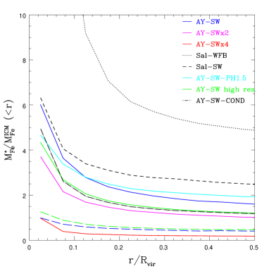
Figure 16: Iron star–to–ICM mass ratios for the different simulations of the “Virgo” cluster. As in Fig. 14, the normal and high resolution AY-SW are shown as well, both uncorrected (solid) and corrected since $z$=2 (long-dashed) for the cooling flow stars.

DELM also point out a correlation between the iron mass within $R_{2500}$ (a region well covered by their profiles) and the X–ray luminosity or temperature. Though few of our simulated clusters overlap with the temperature range of the DELM ones, in Fig. 17 the trend with temperature seems in qualitative agreement with the observed one.

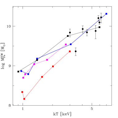
Figure 17: Cumulative Iron masses in the ICM at $R_{2500}$; models shown as squares: AY-SW (blue), AY-SWx2 (magenta), AY-SWx4 (red), COND. (black). Circles: cold–core clusters from De Grandi et al. (2004).

8.2 The Iron Mass-to–Light ratio

A common way of measuring the efficiency of metal production by cluster galaxies is the ICM Iron Mass-to-Light Ratio

$$IMLR_{ICM}\equiv\frac{M^{ICM}_{Fe}}{L_{B}}=\,<Z^{ICM}_{Fe}>\frac{M_{ICM}}{L_{B}}$$ (5)

(Ciotti et al. 1991; Renzini et al. 1993). Observational estimates yield IMLR$\simeq$0.01-0.02 $M_{\odot}/L_{\odot}$, fairly invariant for rich clusters above 2–3 keV (Finoguenov et al. 2000, 2003; DELM). Such a large IMLR indicates a metal production efficiency higher than in the local environment by a factor of 3 or more (Portinari et al. 2004). The above results based on galactic luminosities might however overestimate the actual overall IMLR, and the metal production efficiency, if the contribution of the intra-cluster stars is significant (Lin & Mohr 2004; Zaritsky, Gonzales & Zabludoff 2004).

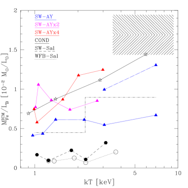
Figure 18: Iron Mass-to-light ratio of the ICM in the B band, from all stars within $R_{500}$. Shaded region: averaged data (along with $1\sigma$-scatter) over nine BeppoSAX nearby rich clusters extrapolated to $R_{500}$, from De Grandi et al. (2004). Step curve: average over ASCA data from Finoguenov et al. (2003). The effect of removing stars formed at the base of the cooling flow since $z=2$ is shown as a dot-longdashed line for the “Virgo” and “Coma” AY-SW simulations.

Fig. 18 illustrates the IMLR of the simulated clusters within $R_{500}$, compared to observational estimates (all scaled to the adopted value of H₀); notice that the BeppoSAX based IMLR of DELM (shaded area) is about twice as large as the ASCA based estimates of Finoguenov et al. (2003; dash-dotted line). Though the BeppoSAX iron profiles are much more accurate, they do not reach as far out as ASCA data and significant extrapolation is required to derive the cumulative iron mass at $R_{500}$, so that the BeppoSAX values should be regarded as upper limits (DELM). As to the IMLR of our simulated clusters, the luminosity is computed considering all stars (both galactic and inter-galactic) within $R_{500}$: in our simulations the distribution of stars is highly skewed toward the cD+intra-cluster stars component, at the expense of the brightest galaxies in the luminosity function (Paper II and III); hence considering only galactic stars in the simulated clusters would seriously bias the luminosity downward. We do however neglect the contribution of the recent star formation at the centre of our cDs where cooling flows onset (Section 2.2): the effect of dropping the luminosity contribution from these innermost young stars is negligible for the lower temperature objects, but turns out to be important for the Virgo and Coma-sized ones (dot-dashed line in Fig. 18).

The IMLR obtained in simulations can be compatible with the observed one if: a) the adopted IMF produces enough metals in the overall; b) the simulations yield the correct partition of metals between the stars and the ICM; c) the star formation history in the simulated cluster is similar to that in real clusters, so that the colours and MLR of the simulated stellar populations are realistic.

The Salpeter simulations evidently have a far too low IMLR in the ICM. Since in principle the Salpeter IMF can produce enough iron to account for the observed enrichment (though not enough $\alpha$–elements, Portinari et al. 2004), the main culprit here is the partition. In the simulations, there is 3-5 times more iron in the stars than in the ICM (Fig. 16); if the expected equipartition (Matteucci & Vettolani 1988; Renzini et al. 1993; Portinari et al. 2004) were reproduced, the iron mass and IMLR of the ICM would be about 3 times larger, hence compatible with at least the ASCA results (step line in Fig. 18). The situation as expected improves with the AY simulations, since this top–heavy IMF both produces more metals and results in stronger feedback and metal dispersion into the ICM (even within the same SW feedback prescription as the Salpeter case).

However, simulations are hardly able to reach the very high levels of IMLR inferred by the BeppoSAX results. Increasing the feedback efficiency to SWx2 and SWx4 evidently increases the IMLR in the ICM, because of the more favourable partition (Fig. 16); nonetheless, as we remarked in the previous section, even if the right level of IMLR were reached, the correct ICM metallicity would not necessarily be achieved in these simulations.

The AY-SW simulations (cooling-flow corrected, with conduction or not) are confirmed to be those that best reproduce the chemical properties of the ICM, including the qualitative trend of decreasing IMLR in poor clusters and groups ($kT\raisebox{-3.8pt}{$\;\stackrel{{\scriptstyle\textstyle<}}{{\sim}}\;$}2$ keV), as a consequence either of strong galactic winds, or of lower enriching efficiency.

8.3 The $\alpha$–elements in the ICM

Mainly produced by SN II, $\alpha$–elements are more direct tracers of star formation and of the massive stars that have enriched the ICM at early times, and also better tracers of the global metallicity — which they dominate by mass. In the ICM $\alpha$–elements are in practice best represented by silicon, the second-best measured element in the ICM after iron; albeit a non–negligible contribution from SNIa, about 80% of the Si production is due to SNII (Portinari et al. 2004).

The [$\alpha$/Fe] abundance ratios in the ICM of rich clusters are supersolar and increase outwards, as $\alpha$ elements have a shallower distribution than iron (Finoguenov et al. 2000; Böhringer et al. 2004; Baumgartner et al. 2005). In particular, they do not mirror the central iron peak in cool core clusters, which is then imputed to SNIa from the central Brightest Cluster Galaxy — in terms of mass, however, this peak represents only a 10% of the global ICM iron content; De Grandi & Molendi 2001; DELM; Böhringer et al. 2004).

Fig. 19 shows that, with the exception of the Sal-WFB simulation where [Si/Fe] is significantly undersolar everywhere, the trend of supersolar [Si/Fe] increasing with radius is present in all our simulations. (The upturn of [Si/Fe] at the very centre in some simulations is due to the recent star formation in the centre of the cD, and is not significant). All the simulations AY-SW and AY-SWx2 also reproduce the correct level of [Si/Fe]; while the Sal-SW and extreme feedback AY-SWx4 simulations have much lower [Si/Fe]. Notice that, although our feedback and enrichment scheme favours the ejection and dispersal of SNII products, SNIa still contribute significantly to the ICM enrichment: for a Salpeter or AY IMF, pure SNII enrichment would correspond to [Si/Fe]$\sim$+0.5, hence, though supersolar, the level of [Si/Fe] in the simulations indicates a significant contribution from SNIa. Actually, for the AY IMF the expected [Si/Fe] for the overall enrichment, including all SNII and SNIa, is [Si/Fe]=+0.2 dex (supersolar since the AY IMF is top–heavy, favouring SNII in proportion to SN Ia); henceforth, for the AY-SW simulations the ICM is enriched by SNII and SNIa in roughly the same proportion as they are in the corresponding IMF.

We can compare our results with those of Tornatore et al. (2004): their simulated cluster is comparable in virial mass to our “Virgo”, and they also present Salpeter and AY IMF simulations with different feedback efficiencies; but their “sub-grid” treatment of star formation and feedback differs from ours. They share our same problem of too steep iron gradients, in all cases; but their abundance ratio profiles behave quite differently from those in Fig. 19. Their [$\alpha$/Fe] is roughly constant, solar or undersolar, over most of the cluster; probably they find lower [$\alpha$/Fe] than we do because their feedback prescription treats SNII and SNIa alike, while ours favours the diffusion of SNII products. Moreover, in the central regions ($R\leq 0.1R_{200}$) they find a peak in [$\alpha$/Fe] due to recent star formation and SNII explosions; indeed their Salpeter models A and B with “standard” wind parameters display profiles very similar to our Sal-WFB simulation. In all our SW simulations, instead, we find at most a mild central enhancement in [$\alpha$/Fe]: our SW feedback prescription seems more efficient at contrasting late star formation at the centre of the cooling flow. Tornatore et al. are able to eliminate such central [$\alpha$/Fe] spikes when invoking additional AGN energy input (Model C), but at the expense of retarding significantly the star formation history — which is not the case in our SW simulations (Paper II). One is then tempted to conclude that their “standard” feedback implementation is as little efficient as our WFB case, and they need to resort to “AGN powering” to eliminate the central spike while we can do it with the sole SNII energy in the SW simulation. But things are not so straightforward: in their model D (AY IMF with “standard” wind paramenters) the high ICM metallicity and [$\alpha$/Fe]$\sim$+0.3 suggest a very efficienct dispersal of metals in the ICM, more than in our AY-SW simulations; their feedback implementation now looks more efficient than our SW one, hence it seems that their scheme is much more sensitive to the underlying IMF. Though more detailed discussion on different implementations is out of the scopes of this paper, we stress the importance of having different algorithms and codes to assess the subtle but important effects of sub-grid physics.

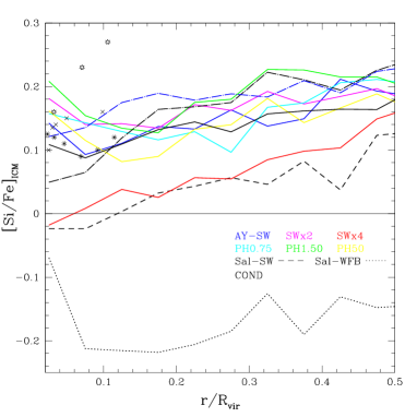
Figure 19: Silicon-over-Iron gradients in the ICM of the two clusters at $z$=0 (“Coma”: dot-dashed). Line colours as in Fig. 14. Data from Finoguenov et al., 2000: two Virgo-sized clusters (Virgo itself, crosses; and A1060, asterisks) and the larger one A3112 (stars).

8.4 The redshift evolution of the ICM metallicity

There is no significant variation in the typical ICM iron abundance of clusters up to $z\simeq 1.2$, implying that the bulk of the enrichment occurs at earlier epochs (Mushotzky & Loewenstein 1997; Donahue et al. 2003; Tozzi et al. 2003). Fig. 20 (top panels) shows that the overall iron abundance, and its profile, in the ICM of simulated clusters is essentially unchanged from $z=0$ to $z=1$, in very good agreement with observations. Any evolution in the ICM metallicity at $z<1$ is limited to the very central regions, $r<0.1R_{vir}$, and is due to the late cooling flows and star formation at the centre of the cD; excluding this effect, since the bulk of the stars in the cluster are formed at $z\raisebox{-3.8pt}{$\;\stackrel{{\scriptstyle\textstyle>}}{{\sim}}\;$}$2 (Papers II and III), at $z$=2 we predict somewhat lower iron metallicities, but such redshift range is not probed by observations yet. The lower panels in the figure show the evolution in [Si/Fe], which as expected decreases in time due to the delayed iron contribution of SNIa with respect to the bulk of the silicon production (from SNII). The change in abundance ratios from $z=0$ to $z=1$ is minor, about 0.1 dex.

There are indications that some evolution in the metallicity of the ICM could be expected due to ram-pressure stripping of the metal richer cold gas from galaxies (Domainko et al. 2006). However, further study of the redshift evolution of metallic abundances and gradients in the ICM (and in the intra-cluster light as well: see Paper III) out of our simulated data is presently on progress.

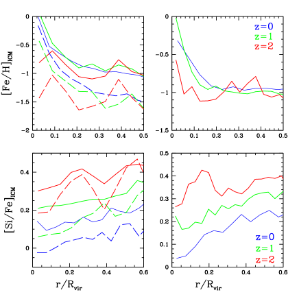
Figure 20: Radial profiles of Iron (top) and Silicon (bottom) abundances in the ICM at z=0,1,2. Left: “Virgo” (solid: AY-SW, dashed: Sal-SW); right: “Coma”. $R_{vir}$ evaluated at z=0.

9 Conclusions

All the results reported are based on cosmological simulations of galaxy clusters including self-consistently cooling, star formation, supernova driven galactic super-winds, chemical evolution, UV field and thermal conduction, as described in Section 2. In relation to modelling the properties of cluster gas and galaxies, especially from the chemical point of view, this represents an important step forward with respect to previous theoretical works on the subject (see also Paper II and III).

In Section 3 the gas distribution has been analysed, in terms of cumulative fractions of baryonic, gas and stellar components. When compared with the “adiabatic” model (no cooling/star formation), the combined effect of cooling and feedback in our simulations makes the gas fraction shift significantly down at all distances. Enhancing feedback, the fraction of gas turned into stars decreases, thus augmenting the cumulative gas fraction up to the virial radius; and at the same time more gas is spread out at larger distances, resulting into a more extended profile (Fig. 1) – this effect becoming even more evident when looking at smaller systems (Fig. 3). From comparing gas distributions reached at $R_{500}$ in systems of different size, we find that feedback and cooling combined together again introduce a trend, with respect to the “adiabatic” run, which is increasing with temperature and which is more prominent in the stronger feedback and in the pre-heating models (Fig. 4); this in turn drives the baryon fraction– temperature correlation, as the stellar fraction seems to follow a fairly constant behaviour which might be compatible with a similarity of the star formation process in systems over a significant mass range.

In modelling the temperature profiles (Section 4), fair agreement has been found with observed distribution from $\sim 0.25R_{vir}$ outwards, while an extended isothermal core and the positive gradient in the innermost regions ($r<0.1R_{vir}$) are still lacking in most models; feedback and pre–heating help to smooth out the steep negative temperature gradient typical of simulations with cooling, yet the temperature profile remains more sharply peaked than the observed one (Fig. 5). Thermal conduction is found to affect the higher temperature, more massive systems in such a way that outer radial temperature gradients are reduced and “cold fronts” are smoothed out.

As for the entropy profiles, we needed to appeal to the most extreme SWx4 scheme in order to lower the central density to values consistent with the presence of an entropy-floor at $\sim 100$keV$\cdot$cm², and even higher in the smaller-scales simulated systems. The observed level and slope of the $L_{X}-T$ relation are also best reproduced by strenghtening the feedback up to the SWx4 case, at least in the probed range 1-6 keV; otherwise, the low-entropy gas at the cluster’s centre induces over-emissivity, as seen in other simulations. Although general results from temperature and entropy distributions still call for the need of balancing cooling by enhancing feedback, it is however a firm result that our AY-SW models can actually fit cold-core systems, reproducing observed values of central entropy at 10-20 keV$\cdot$cm².

The findings on the mass-to-light ratio of the ICM and the cold fraction place both in a fair agreement with observations, when adopting the standard SW scheme for stellar feedback with a top-heavy IMF, while a Salpeter IMF yields too large stellar fractions and masses, giving rise to an excess optical luminosity –as it is evident from the radial profiles (Fig. 13). The cold fraction scales with cluster size, decreasing as system mass or temperature increases, as observed; in the simulations this trend is due to the more extended gas distribution, and the smaller gas and baryonic fraction within $R_{500}$, characterizing systems of lower mass and temperature, rather than to an increase in the efficiency of galaxy formation and in the stellar fraction.

In Section 8 the metal enrichment of the ICM has been analysed. It has been found that the iron abundance profiles show a steep inner gradient, and an iron abundance overall level which is somewhat low relative to observations, at least at $r\ga 0.1R_{vir}$. The steep inner gradient, along with the high iron level within this inner part, is mostly due to the excessive star formation, with subsequent chemical evolution, resulted from the spurious, late-time central cooling flows. This problem would be cured, if e.g. some non-supernova related feedback mechanisms could be invoked for halting the cooling flows (see below).

Regarding the overall level of iron abundance, it is clear from our results that adopting a top-heavier IMF such as Arimoto-Yoshii rather than a Salpeter one, helps to improve the distribution considerably. Enhancing the feedback then helps to balance the partition between metals in stars and in the ICM, favouring a higher iron MLR of the ICM, but this comes at the expense of hampering star formation and metal production itself, resulting in a too low metallicity for the ICM. Rather than a stronger stellar feedback, an improved understanding of the cooling and heating processes in the very central regions and of the formation of the cD seems to be the key to better balancing the total iron content of the stars and ICM. In fact, when excluding from the stellar iron mass the iron produced by stars formed at the base of the cooling flow, the metal partition between stars and ICM gets skewed in favour of the latter, thus much closer to empirical estimates. Then realistic values of metal enrichment through the ICM are attained, as seen from the cumulative iron masses in “Coma” and “Virgo” modelled and well reproduced by AY-SW scheme (Fig. 15). And at the same time, such cooling flow correction helps the cold fraction as well to get reduced to values lower than 20%, excellently matching those observed (Figs. 12-13).

Besides iron, the distribution of silicon as tracer of $\alpha$-elements from SNII in the ICM shows a non-constant, increasing radial trend with respect to iron abundance, where the AY-SW model is fairly efficient in preventing the central peak due to recent star formation, as is clear from comparison with the WFB case (Fig. 19). Although the evolution of the thermal and chemical properties of the ICM over significant redshift ranges will be in perspective treated in another forthcoming paper, here we just stress the attention upon the behaviour of gas metal abundances since $z$=2: iron levels appear to remain essentially unchanged at least from $z$=1 to the present; silicon abundance with respect to iron instead decreases due to the delayed contribution of SNIa (Fig. 20).

In summary, although we can reproduce many observed features of groups and clusters, our results point out the need of a general heating mechanisms which could be able to suppress the overproduction of stars at late times in the central cluster regions, without affecting the overall cluster star formation. Hot unstable buoyant bubbles as observed in X–ray (e.g. Ensslin & Heinz, 2002 for a model), released in association with AGN jets, can transport energy by convection, thus providing a means of keeping the central gas from cooling. Another possibility is that the ICM might contain random magnetic fields of sufficient strength to significantly reduce the gas inflow by the combined effect of magnetic pressure and reconnection. Yet another option could be dissipation of sound waves resulting from AGN induced, turbulent motions, as recently proposed by Fujita & Suzuki (2005).

References

- (1) Abadi M.G., Navarro J.F., Steinmetz M., Eke V.R., 2003, ApJ 591, 499
- (2) Aguirre A., Hernquist L., Schaye J., Katz N., Weinberg D.H., Gardner J., 2001, ApJ 561, 521
- (3) Allen S.W., Fabian A.C., 1998, MNRAS 297, L57
- (4) Allen S.W., Fabian A.C., Johnstone R.M., Arnaud K.A., Nulsen P.E.J., 2001, MNRAS 322, 589
- Antonuccio et al. (2003) Antonuccio-Delogu V., Becciani U., Ferro D., 2003, Comput. Phys. Commun. 155, 159
- (6) Arimoto N., Yoshii Y., 1987, A&A 173, 23
- Arnaud et al. (1992) Arnaud M., Rothenflug R., Boulade O., Vigroux L., Vangioni–Flam E., 1992, A&A 254, 49
- Arnaud and Evrard (1999) Arnaud M., Evrard A.E., 1999, MNRAS 305, 631
- Arnaud et al. (2001) Arnaud M., et al. 2001, A&A 365, L67
- Babul et al. (2002) Babul A., Balogh M.L., Lewis G.F., Poole G.B., 2002, MNRAS 330, 329
- Balogh et al. (1999) Balogh M.L., Babul A., Patton D.R., 1999, MNRAS 307, 463
- Balogh et al. (2001) Balogh M.L., Pearce F.R., Bower R.G., Kay S.T., 2001, MNRAS 326, 1228
- (13) Baumgartner W.H., Loewenstein M., Horner D.J., Mushotzky R.F., 2005, ApJ 620, 680
- (14) Bell E.F., de Jong R.S., 2001, ApJ 550, 212
- (15) Bialek J.J., Evrard A.E., Mohr J.J., 2001, ApJ 555, 597
- (16) Böhringer H., Matsushita K., Churazov E., Finoguenov A., Ikebe Y., 2004, A&A 416, L21
- Borgani et al. (2001) Borgani S., et al., 2001, ApJ 559, 71
- Borgani et al. (2002) Borgani S., et al., 2002, MNRAS 336, 409
- Borgani et al. (2004) Borgani S., et al., 2004, MNRAS 348, 1078
- (20) Bower R.G., 1997, MNRAS 288, 355
- (21) Bower R.G., Benson A.J., Lacey C.G., Baugh C.M., Cole S., Frenk C.S., 2001, MNRAS 325, 497
- (22) Boyle B.J., Terlevich R.J., 1998, MNRAS 239, L49
- (23) Brighenti F., Mathews W.G., 2001, ApJ 553, 103
- (24) Carilli C.L., Taylor G.B., 2002, ARofA&A 40, 319
- (25) Cavaliere A., Fusco-Femiano R., 1976, A&A 49, 137
- (26) Cavaliere A., Menci N., Tozzi P., 1997, ApJ 484, L21
- (27) Cavaliere A., Menci N., Tozzi P., 1998, ApJ 501, 493
- (28) Cavaliere A., Lapi A., Menci N., 2002, ApJ 581, L1
- (29) Cen R., Ostriker J.P., 1994, ApJ 429, 4
- (30) Ciotti L., Ostriker J.P., 1997, ApJ 487, L105
- (31) Ciotti L., Ostriker J.P., 2001, ApJ 551, 131
- (32) Ciotti L., D’Ercole A., Pellegrini S., Renzini A., 1991, ApJ 376, 380
- (33) Cleary P.W., Monaghan J.J., 1990, ApJ 349, 150
- (34) Cowie L.L., McKee C.F., 1977, ApJ 211, 135
- (35) Croton D.J., Springel V., White S.D.M., et al., 2006, MNRAS 365, 11
- (36) Davè R., et al., 2001, ApJ 552, 473
- (37) Davè R., Katz N., Weinberg D.H., 2002, ApJ 579, 23
- (38) David L.P., Arnaud K.A., Forman W., Jones C., 1990, ApJ 356, 32
- (39) David L.P., Jones C., Forman W., 1992, ApJ 388, 82
- (40) David L.P., Slyz A., Jones C., Forman W., Vrtilek S.D., Arnaud K.A., 1993, ApJ 412, 479
- (41) David L.P., Jones C., Forman W., 1995, ApJ 445, 578
- De Grandi et al. (2003) De Grandi S., Ettori S., Longhetti M., Molendi S., 2004, A&A 419, 7 (DELM)
- De Grandi and Molendi (2001) De Grandi S. and Molendi S., 2001, ApJ 551, 153
- De Grandi and Molendi (2002) De Grandi S., Molendi S., 2002, ApJ 567, 163
- (45) Dekel A., Silk J. 1986, ApJ 303, 39
- (46) Domainko W., Gitti M., Schindler S., Kapferer W., 2004, A&A 425, L21
- (47) Domainko W., et al., 2005, A&A 452, 795
- (48) Donahue M. and ROXS Collaboration, 1999, ApJ 527, 525
- (49) Donahue M., Gaskin J.A., Patel S.K., Joy M., Clowe D., Hughes J.P., 2003, ApJ 598, 190
- (50) D’Onghia E., Sommer–Larsen J., Romeo A.D., Burkert A., Pedersen K., Portinari L., Rasmussen J., 2005, ApJL 630, L109
- (51) Edge A.C, Stewart G.C., 1991, MNRAS 252, 414
- Eisenstein & Hut (1998) Eisenstein D. J., & Hut P., 1998, ApJ 498, 137
- (53) Eke V.R., Navarro J.F., Frenk C., 1998, Apj 503, 569
- Eldridge and Tout (2004) Eldridge J.J., Tout C.A., 2004, MNRAS 353, 87
- (55) Ensslin T.A., Heinz S., 2002, A&A 384, 27
- Ettori et al. (2002) Ettori S., De Grandi S, Molendi S., 2002, A&A 391, 841
- (57) Ettori S., Fabian A.C., 2000, MNRAS 317, 57
- Evrard1 (1990) Evrard A.E., 1990, ApJ 363, 349
- Evrard2 (1996) Evrard A.E., Metzler Ch.A., Navarro J.F., 1996, ApJ 469, 494
- Evrard3 (1991) Evrard A.E., Henry J.P., 1991, ApJ 383, 95
- (61) Fabian A.C., 1994, ARofA&A 32, 277
- (62) Finoguenov A., Ponman T.J., 1999, MNRAS 305, 325
- Finoguenov et al. (2000) Finoguenov A., David L.P., Ponman T.J., 2000, ApJ 544, 188
- (64) Finoguenov A., Jones C., Böhringer H., Ponman T.J., 2002, ApJ 578, 74
- Finoguenov et al. (2003) Finoguenov A., Burkert A., Böhringer H., 2003, ApJ 594, 136
- (66) Franceschini A. et al., 2003, MNRAS 343, 1181
- (67) Frenk C.S. et al., 1999, ApJ 525, 554
- (68) Fujita Y., Suzuki T.K., 2005, ApJ 630, L1
- (69) Fukazawa Y., Makishima K., Tamura T., Ezawa H., Xu H., Ikebe Y., Kikuchi K., Ohashi T., 1998, PASJ 50, 187
- (70) Gelato S., Sommer-Larsen J., 1999, MNRAS 303, 321
- (71) Gerhard O., Kronawitter A., Saglia R.P., Bender R., 2001, AJ 121, 1936
- (72) Gerritsen J.P.E., 1997, Ph.D. thesis, Kapetyn Astron. Inst.
- Governato et al. (2004) Governato F. et al. 2004, ApJ 607, 688
- (74) Haardt F., Madau P., 1996, ApJ 461, 20
- Helsdon and Ponman (2000a) Helsdon S.F., Ponman T.J., 2000a, MNRAS 315, 356
- Helsdon and Ponman (2000b) Helsdon S.F., Ponman T.J., 2000b, MNRAS 319, 933
- (77) Jubelgas M., Springel V., Dolag K., 2004, MNRAS 351, 423
- (78) Kaiser N., 1991, ApJ 383, 104
- (79) Kapferer W., et al., 2006, A&A 447, 827
- (80) Katz N., White S.D.M., 1993, ApJ 412, 455
- (81) Kay S.T., Thomas P.A., Theuns T., 2003, MNRAS 343, 608
- (82) Kay S.T., Thomas P.A., Jenkins A., Pearce F.R., 2004, MNRAS 355, 1091
- (83) Knight P.A., Ponman T.J., 1997, MNRAS 289, 955
- (84) Kravtsov A.V., Nagai D., Vikhlinin A.A., 2005, ApJ 325, 588
- (85) Kravtsov A.V., Yepes G., 2000, MNRAS 318, 227
- (86) Larson R.B., 1974, MNRAS 169, 229
- (87) Lewis G.F., Babul A., Katz N., Quinn Th., Hernquist L., Weinberg D.H., 2000, ApJ 536, 623
- Lia et al. (2002a) Lia C., Portinari L., Carraro G., 2002, MNRAS 330, 821
- Lin et al. (2003) Lin Y., Mohr J., Stanford S.A., 2003, ApJ 591, 749 (LMS)
- Lin & Mohr (2004) Lin Y.-T., Mohr J.J., 2004, ApJ 617, 879
- (91) Lloyd-Davies E.J., Ponman T.J., Cannon D.B., 2000, MNRAS 315, 689
- (92) Loewenstein M., Mushotzky R.F., 1996, ApJ 466, 695
- (93) Loewenstein M., 2001, ApJ 557, 573
- (94) Lou Y., Bian F., 2005, MNRAS 358, 1231
- (95) Mac Low, M.-M., Ferrara, A. 1999, ApJ 513, 142
- Markevitch (1998) Markevitch M., 1998, ApJ 504, 27
- (97) Markevitch M. et al., 2000, ApJ 541, 542
- (98) Matteucci F., Vettolani G., 1988, A&A 202, 21
- (99) McCarthy I.G., Balogh M.L., Babul A., Poole G.B., Horner D.J., 2004, ApJ 613, 811
- (100) McNamara B.R. et al., 2000, ApJ 534, L135
- (101) Menci N., Cavaliere A., 2000, MNRAS 311, 50
- (102) Metzler C.A., Evrard A.E., 1994, ApJ 437, 564
- (103) Mo H. J., Mao S., 2002, MNRAS 333, 768
- (104) Monaghan J. J., Lattanzio J. C. 1985, A&A 149, 135
- (105) Moretti A., Portinari L., Chiosi C., 2003, A&A 408, 431
- (106) Mori M., Yoshii Y., Tsujimoto T., Nomoto, K. 1997, ApJ 478, L21
- (107) Mushotzky R.F., 1984, PhScrT 7, 157
- (108) Mushotzky R.F., Loewenstein M., 1997, ApJ 481, L63
- (109) Nagai D., Kravtsov A.V., 2004, in Outskirts of galaxy clusters, IAU Coll. 195, eds. A. Diaferio et al., p.296
- (110) Narayan R., Medvedev M.V., 2001, ApJ 562, L129
- (111) Navarro J.F, Frenk C., White S.D.M., 1995, MNRAS 275, 720
- (112) Pearce F.R., Thomas P.A., Couchman H.M.P., Edge A.C., 2000, MNRAS 317, 1029
- (113) Persic M., Rephaeli Y., 2002, A&A 382, 843
- Piffaretti et al. (2005) Piffaretti R., Jetzer P., Kaastra J. S., Tamura T., 2005, A&A 433, 101
- (115) Pipino A., Matteucci F., Borgani S., Biviano A., 2002, NewA 7, 227
- (116) Ponman T.J., Bourner P.D.J., Ebeling H., Bohringer H., 1996, MNRAS 283, 690
- (117) Ponman T.J., Cannon D.B., Navarro J.F., 1999, Nature 397, 135
- Ponman et al. (2003) Ponman T.J., Sanderson A.J.R., Finoguenov A., 2003, MNRAS 343, 331
- Portinari et al. (1998) Portinari L., Chiosi C., Bressan A., 1998, A&A 334, 505
- Portinari et al. (2004) Portinari L., Moretti A., Chiosi C., Sommer–Larsen J., 2004, ApJ 604, 579
- (121) Portinari L., 2005, in Modelling the Intergalactic and Intracluster Media, V. Antonuccio et al. (eds.), MemSAIt Suppl. in press (astro-ph/0402486)
- (122) Pratt G.W., Arnaud M., 2003, A&A 408, 1
- (123) Ranalli P., Comastri A., Setti G., 2003, A&A 399, 39
- Rasmussen and Ponman (2004) Rasmussen J., Ponman T.J., 2004, MNRAS 349, 722
- Rasmussen et al. (2004) Rasmussen J., Sommer-Larsen J., Toft S., Pedersen K., 2004, MNRAS 349, 255
- (126) Recchi S., Matteucci F., D’Ercole A., 2001, MNRAS 322, 800
- Renzini1 (1997) Renzini A., 1997, ApJ 488, 35
- (128) Renzini A., 2004, in Clusters of galaxies, ed. J.S. Mulchaey, A. Dressler & A. Oemler (Cambridge University Press), p. 260
- (129) Renzini A., Ciotti L., D’Ercole A., Pellegrini S., 1993, ApJ 419, 52
- (130) Ritossa C., Garcia-Berro E., Iben I.Jr., 1996, ApJ 460, 489
- (131) Ritossa C., Garcia-Berro E., Iben I.Jr., 1999, ApJ 515, 381
- Robertson et al. (2004) Robertson B., Yoshida N., Springel V., Hernquist L. 2004, ApJ 606, 34
- (133) Romano D., Silva L., Matteucci F., Danese L., 2002, MNRAS 334, 444
- PaperII (2005) Romeo A.D., Portinari L., Sommer-Larsen J., 2005, MNRAS 361, 983 (Paper II)
- Roussel et al. (2000) Roussel H., Sadat R., Blanchard A., 2000, A&A 361, 429
- (136) Salpeter E.E., 1955, ApJ 121, 161
- Sanderson et al. (2003) Sanderson A.J.R., Ponman T.J., Finoguenov A., Lloyd-Davies E.J., Markevitch M., 2003, MNRAS 340, 989
- (138) Scannapieco C., Tissera P.B., White S.D.M., Springel V., 2005, MNRAS 364, 552
- (139) Schindler S., et al., 2005, A&A 435, L25
- (140) Silk J., Rees M. J. 1998, A&A 331, L1
- Sommer-Larsen et al. (2003) Sommer-Larsen J., Götz M., Portinari L., 2003, ApJ 596, 47 (SLGP)
- PaperIII (2005) Sommer-Larsen J., Romeo A.D., Portinari L., 2005, MNRAS 357, 478 (Paper III)
- Springel and Hernquist (2002) Springel V., Hernquist L., 2002, MNRAS 333, 649
- (144) Springel V., Di Matteo T., Hernquist L., 2005, ApJ 620, L79
- (145) Suginohara T., Ostriker J.P., 1998, ApJ 507, 16
- (146) Sutherland R.S., Dopita M.A., 1993, ApJS 88, 253 (SD)
- (147) Tamura T., Kaastra J.S., den Herder J.W.A., Bleeker J.A.M., Peterson J.R., 2004, A&A 420, 135
- (148) Thacker R. J., Couchman H. M. P. 2000, ApJ 545, 728
- (149) Thacker R. J., Couchman H. M. P. 2001, ApJ 555, L17
- Thomas & Couchman (1992) Thomas P.A., Couchman H.M.P., 1992, MNRAS 257, 11
- (151) Thomas P.A., Muanwong O., Kay S.T., Liddle A.R., 2002, MNRAS 330, L48
- Tornatore et al. (2003) Tornatore L., Borgani S., Springel V., Matteucci F., Menci N., Murante G., 2003, MNRAS 342, 1025
- Tornatore et al. (2004) Tornatore L., Borgani S., Matteucci F., Recchi S., Tozzi P., 2004, MNRAS 349, L19
- (154) Tozzi P., Norman C., 2001, ApJ 546, 63
- (155) Tozzi P., Rosati P., Ettori S., Borgani S., Mainieri V., Norman C., 2003, ApJ 593, 705
- VS (1) Valageas P., Silk J., 1999a, A&A, 347, 1
- VS (2) Valageas P., Silk J., 1999b, A&A, 350, 725
- Valdarnini (2003) Valdarnini R., 2003, MNRAS 339, 1117
- (159) Vikhlinin A., Forman W., Jones C., 1999, ApJ 525, 47
- (160) Voigt L.M., Fabian A.C., 2004, MNRAS 347, 1130
- (161) Voigt L.M., Schmidt R.W., Fabian A.C., Allen S.W., Johnstone R.M., 2002, MNRAS 335, L7
- Voit & Bryan (2001) Voit G.M., Bryan G.L., 2001, Nature 414, 425
- Voit et al. (2002) Voit G.M., Bryan G.L., Balogh M.L., Bower R.G., 2002, ApJ 576, 601
- Voit et al. (2003) Voit G.M., Balogh M.L., Bower R.G., Lacey C.G., Bryan G.L., 2003, ApJ 593, 272
- (165) Yamada M., Fujita Y., 2001, ApJ 553, L145
- White et al. (1993) White S.D.M., Navarro J.F., Evrard A.E., Gnedin N., 1993, Nature 366, 429
- Wu et al. (2000) Wu K.K.S., Fabian A.C., Nulsen P.E.J., 2000, MNRAS 318, 889
- (168) Zanni C., Murante G., Bodo G., Massaglia S., Rossi P., Ferrari A., 2005, A&A 429, 399
- Zaritsky, Gonzalez & Zabludoff (2004) Zaritsky, D., Gonzalez, A.H, & Zabludoff, A.I., 2004, ApJ, 613, L93