Challenges for Precision Cosmology with X-ray and Sunyaev-Zeldovich Effect Gas Mass Measurements of Galaxy Clusters

Abstract

We critically analyze the measurement of galaxy cluster gas masses, which is central to cosmological studies that rely on the galaxy cluster gas mass fraction. Using synthetic observations of numerically simulated clusters viewed through their X-ray emission and thermal Sunyaev-Zeldovich effect (SZE), we reduce the observations to obtain measurements of the cluster gas mass. We utilize both parametric models such as the isothermal cluster model and non-parametric models that involve the geometric deprojection of the cluster emission assuming spherical symmetry. We are thus able to quantify the possible sources of uncertainty and systematic bias associated with the common simplifying assumptions used in reducing real cluster observations including isothermality and hydrostatic equilibrium. We find that intrinsic variations in clusters limit the precision of observational gas mass estimation to $\sim$10% to $1\sigma$ confidence excluding instrumental effects. Gas mass estimates performed via all methods surprisingly show little or no trending in the scatter as a function of cluster redshift. For the full cluster sample, methods that use SZE profiles out to roughly the virial radius are the simplest, most accurate, and unbiased way to estimate cluster mass. X-ray methods are systematically more precise mass estimators than are SZE methods if merger and cool core systems are removed, but X-ray methods slightly overestimate (5-10%) the cluster gas mass on average. SZE methods are more precise and accurate than X-ray methods at mass estimation if the sample is contaminated by merging, disturbed, or cool core clusters. In fact we find that cool core clusters in our samples are particularly poor candidates for observational mass estimation, even when excluding emission from the core region. The effects of cooling in the cluster gas alter the radial profile of the X-ray and SZE surface brightness outside the cool core region, leading to poor gas mass estimates in cool core clusters. Finally, we find that methods using a universal temperature profile estimate cluster masses to higher precision than those assuming isothermality.

1. Introduction

Measuring the apparent change of cluster gas fraction with redshift produces constraints on the dark energy equation of state, $w$ (e.g. Pen (1997), Sasaki (1996), Rines et al. (1999), Vikhlinin et al. (2005)). Determining cluster gas fractions requires high precision estimation of cluster gas mass and total mass from observables. In order for such methods to provide strong constraints on cosmological parameters, cluster mass estimators must be accurate to $\sim$10% (Haiman et al., 2001). Previous studies (e.g. Evrard et al. (1996)) suggest that this level of precision may be difficult to achieve. The often used scaling relation between cluster total mass and X-ray spectral temperature has relatively small scatter compared to other methods, but the normalization is still uncertain to $\sim$30% (e.g. Sanderson et al. (2003)). Additionally, using X-ray observations and the assumption of hydrostatic equilibrium appears to lead to a bias in cluster total mass estimates (Rasia et al., 2006). While it is necessary to estimate both the cluster gas and total mass to determine the gas fraction, this study aims first to determine the limiting accuracy of various X-ray and Sunyaev-Zeldovich effect (SZE) observational methods of cluster gas mass estimation. This analysis will help determine whether cluster methods can be accurate enough to do precision cosmology. This study addresses the key question: What is the best way to measure cluster gas masses with precision in order to do cosmology?

High resolution X-ray or SZE observations of clusters coupled with assumptions about the gas distribution lead to estimates of the gas mass in the cluster dark matter potential well. The electron number density is often assumed to fit a $\beta$ model,

$$n_{e}(r)=n_{e0}\left(1+\left(\frac{r}{r_{c}}\right)^{2}\right)^{-3\beta/2}.$$ (1)

Fitting an observed X-ray or SZE profile to these projected $\beta$ model X-ray surface brightness and SZE $y$ parameter distributions results in a description of the density distribution, which can be integrated to obtain the gas mass. The difference in dependence on gas density and temperature of X-ray emissivity and the SZE $y$ parameter makes the combination of these two methods of observation very powerful. Because of this difference, the observability of clusters via each method is affected differently by the impact of central physics including radiative cooling and feedback mechanisms, as well as the transient boosting of surface brightness and spectral temperature generated during merging events. Thus these two methods not only select a different sample of clusters, but combined SZE/X-ray observations of individual clusters allow one to extract the density and temperature of the gas without relying on X-ray spectral temperatures.

Recent numerical (e.g. Loken et al. (2002)) and observational studies (e.g. Vikhlinin et al. (2005)) suggest that the cluster gas is not isothermal, but fits more closely to a universal temperature profile (UTP), for this study written as

$$T(r)=\langle T\rangle_{500}T_{0}\left(1+\left(\frac{r}{\alpha r_{500}}\right)^{2}\right)^{-\delta},$$ (2)

where $\langle T\rangle_{500}$ is the average temperature inside a projected overdensity radius of $r_{500}$. Here the subscript indicates that the ratio of the average overdensity inside this radius with respect to the comoving universal mean is equal to 500. $T_{0}$, $\alpha$, and $\delta$ are parameters whose mean value is measured from the entire cluster population at some redshift. We perform a deprojection of the X-ray and SZE profiles and use this additional assumption about the gas temperature to calculate the density profile and the mass.

With observations of both X-ray and SZE for a particular cluster, an observer can deproject the surface brightness of each simultaneously to determine the gas density. This method is particularly powerful due to the difference in dependence of X-ray and SZE emission on density and temperature. With combined observations, one can in principle determine the cluster gas mass with no assumptions about the cluster temperature profile, using only the weaker assumption of spherical symmetry in the deprojection. In this study, we also perform such a combined deprojection of X-ray and SZE profiles to obtain the gas density radial profile with no assumption about the temperature profile.

We examine the effect of the assumption of the gas temperature and density profile on the determination of the true cluster gas mass. Using adaptive mesh hydro/N-body cosmological simulations, we have extracted clusters with $M\geq 10^{14}M_{\odot}$ out to a redshift of z = 2. This sample has $\sim$100 such clusters at z=0 and $\sim$10 clusters at z = 2. For each cluster, we have fit the X-ray and SZE surface brightness profiles to those produced by a best-fit $\beta$-model gas distribution. We also perform a direct geometric deprojection of the SZE and X-ray surface brightness. We analyze them separately assuming the gas temperature follows a UTP, as well as jointly with no assumptions about the temperature distribution to determine a density profile and thus the mass. The joint method requires spatially resolved X-ray and SZE profiles for each cluster and assumes only spherical symmetry. We also compare profile methods with cluster X-ray and SZE scaling relations for accuracy in mass determination.

The outline of this work is as follows: Section 2 describes the numerical simulations performed, Section 3 details the methods of observational cluster gas mass estimation used, Section 4 contains results of that mass estimation, and Section 5 states conclusions.

2. Simulations

The simulations described here use the cosmological hydro/N-body adaptive mesh refinement (AMR) code Enzo (O’Shea et al. (2005); http://cosmos.ucsd.edu/enzo) to evolve both the dark matter and baryonic fluid in the clusters utilizing the piecewise parabolic method (PPM) for the hydrodynamics. We achieve a peak resolution of 15.6$h^{-1}$kpc with seven levels of refinement. Refinement of high density regions is done as described in Motl et al. (2004). We assume a concordance $\Lambda$CDM cosmological model with the following parameters: $\Omega_{b}=0.026,\Omega_{m}=0.3,\Omega_{\Lambda}=0.7,h=0.7,$ and $\sigma_{8}=0.928$.

The simulations used for this study were briefly described in Motl et al. (2005). The same four sets of simulation data are used here, including progressively more baryonic physics. The baseline simulation was run with purely adiabatic physics for the baryons. The other three simulations add radiative cooling, star formation, and star formation with a moderate amount of thermal feedback from supernovae using the Cen & Ostriker (1992) algorithm. The radiative cooling is calculated via a Raymond-Smith model for the X-ray emission.

3. Methods of Gas Mass Estimation

We use the catalog of AMR refined clusters identified in each simulation volume which was described in Motl et al. (2005). Each catalog from the four simulations contains $\approx$ 100 clusters from the current epoch in the mass range $10^{14}M_{\odot}\leq M\leq 2\times 10^{15}M_{\odot}$ ($\sim 15$% of Virgo mass to $\sim$Coma mass) and also contains all clusters above $10^{14}M_{\odot}$ for a series of twenty redshift bins out to $z=2$. This corresponds to roughly 1500 clusters in the interval $0<z<2$ in each catalog.

Our objective was to determine the reliability of observational cluster mass estimation methods. We examine the relative accuracy of these methods with the cluster observables in their simplest form, uncontaminated by instrumental effects. This allows us to determine the limiting accuracy of any particular method for a realistic, mass-limited set of clusters in a cosmological environment. In order to perform a mass estimation for these clusters in a method similar to that done observationally, we first generate projected maps of each cluster volume of their X-ray surface brightness and SZE y parameter. The X-ray surface brightness at any point in the projected map is generated by integrating along the line of sight the bremsstrahlung emissivity

$$S_{X}=\frac{1}{4\pi(1+z)^{4}}\int n_{e}(l)n_{H}(l)\Lambda(T(l))dl$$ (3)

where $\Lambda$ is the emission function for the cluster gas. Generally this will include thermal bremsstrahlung emission in addition to spectral line emission. For most of this study, $\Lambda$ is simply

$$\Lambda(T)=\Lambda_{0}T^{1/2},$$ (4)

which is a simple approximation to the X-ray emission representing the thermal bremsstrahlung which dominates massive clusters with high virial temperatures ($>$ 2 keV). However, for a subset of the clusters evolved to z=0, we have calculated the thermal emissivity via a Raymond-Smith model assuming a metallicity of 0.3 of the solar value (Brickhouse et al., 1995).

The SZE Compton $y$ parameter is calculated on each line of sight as (Sunyaev & Zeldovich, 1972),

$$y=\int\sigma_{T}n_{e}(l)\frac{k_{b}T(l)}{m_{e}c^{2}}dl.$$ (5)

One additional map that is very helpful in mass estimation is that of the spectral temperature. In this study we have used the emission weighted temperature as

$$T_{ew}=\frac{\int[n_{e}n_{H}\Lambda(T)]Tdl}{\int n_{e}n_{H}\Lambda(T)dl}.$$ (6)

For our subset of z=0 clusters for which we have generated Raymond-Smith emissivities to calculate the X-ray surface brightness, we have used a projected “spectroscopic-like temperature” ($T_{sl}$ as in Rasia et al. (2005)). This value for the projected temperature more closely approximates the spectral temperature of the cluster that would be determined from the X-ray spectrum. The value of $T_{sl}$ used here is

$$T_{sl}=\frac{\int n_{e}n_{H}T^{a}/T^{1/2}dl}{\int n_{e}n_{H}T^{a}/T^{3/2}dl},$$ (7)

where a=0.75 is a fitted parameter from Rasia et al. (2005).

From the simulation data, we are able to generate these three maps at three orthogonal orientations of the cluster. We then have spatially resolved images and spectral temperatures for each cluster. From these maps, we can use typical observational techniques to estimate the cluster gas mass, and compare to the true mass of each cluster on the simulation grid. For this study we have restricted ourselves to methods which require only radial profiles of the surface brightness and average spectral (emission-weighted) temperature. X-ray methods that use spectral temperature profiles require much deeper observations in order to achieve good photon statistics at large radius, and therefore are costly observations for large cluster samples.

3.1. Beta Models

As in Eq. 1, the gas density distribution is often described as a beta model (Cavaliere & Fusco-Femiano, 1978). A beta model density distribution results in an X-ray projected radial surface brightness distribution of the form

$$S_{X}(r)=S_{X0}\left(1+\left(\frac{r}{r_{c}}\right)^{2}\right)^{\frac{1}{2}-3\beta}$$ (8)

where

$$S_{X0}\propto n_{e0}^{2}\langle T\rangle^{\frac{1}{2}}.$$ (9)

This proportionality holds in the bremsstrahlung limit, but the temperature dependence is weaker in a fixed X-ray band (Mohr et al., 1999). In the above relation, $n_{e0}$ is the central density normalization of the beta model, and $\langle T\rangle$ indicates the average spectral temperature inside a given radius. Similarly for the SZE, a beta model density distribution results in a projected radial distribution of the Compton $y$ parameter

$$y(r)=y_{0}\left(1+\left(\frac{r}{r_{c}}\right)^{2}\right)^{\frac{1}{2}-\frac{3\beta}{2}}$$ (10)

where

$$y_{0}\propto n_{e0}\langle T\rangle.$$ (11)

Note particularly the stark difference in dependence on density and temperature for the X-ray surface brightness and Compton $y$ parameter. This difference contributes to the subsequent variation in the quality of mass estimates using X-ray or SZE methods.

Bolstered by earlier observational evidence, the hot gas in clusters is commonly assumed to be isothermal (e.g., Shimizu et al. (2003)). In the isothermal case, the $\beta$-model has a physical interpretation, namely it is the density profile which approximates an isothermal King model (King, 1966, 1972). By fitting isothermal $\beta$-model relations to radial profiles of X-ray surface brightness and Compton $y$ parameter, respectively, we obtain a value for $\beta$, as well as a normalization of the profile. We use an average spectral temperature (in this case emission weighted temperature) to then calculate a value for $n_{e0}$. Integrating the density profile then results in an estimate of the gas mass for each cluster.

3.2. Universal Temperature Profile Methods

It has been shown both in our simulations (Loken et al., 2002) and in X-ray observations (Vikhlinin et al., 2005) that hot gas in many clusters is not isothermal, but follows a universal temperature profile (UTP) where temperature declines with radius. We have also performed mass estimates using the assumption of a UTP in the cluster gas. The method of mass estimation in this case involves a geometric deprojection of the cluster radial surface brightness or Compton $y$ parameter distribution. This deprojection is performed in a similar way to previous studies, via the method of Kriss et al. (1983), originally described in Fabian et al. (1981), seen more recently in Buote (2000). Under the assumption of spherical symmetry, the emissivity as a function of radius in three dimensions can be recovered by recognizing that the luminosity of each projected annulus of the cluster results from contributions from spherical shells which overlap one another.

For the X-ray, the emissivity profile can be converted to a density profile, provided one knows the temperature in each shell. This information is provided by the UTP, the normalization of which is set by the value for the average projected emission weighted temperature inside $r_{500}$. Similarly for the SZE, one can calculate the value of Compton $y$ per unit volume in each shell, and with a temperature from UTP, extract the density in each shell. Then, in either the case of X-ray deprojection or SZE deprojection, we simply add up the mass in the shells out to some fiducial radius to get the total gas mass. In the X-ray method, one also has the option of simultaneously deprojecting the spectral temperature to get a three-dimensional temperature profile, calculating the mass in that way. This method is limited due to the necessity of a large number of photon counts in bins at large radius.

3.3. Joint SZE/Xray Methods

Ideally, if one has both an X-ray and SZE profile of each cluster, one need not make any assumption about cluster temperature. Due to the different dependence of SZE and X-ray emissivity on density and temperature, a profile of each can be used to eliminate the temperature dependence (e.g. Patel et al. (2000)). With deprojected X-ray and SZE profiles, we are able to directly calculate the density profile with no reliance on UTP or any information about temperature whatsoever. We have also calculated mass estimates in this way for each cluster in our simulated dataset.

3.4. Scaling Relations

For completeness, we should mention that cluster total mass is often deduced from X-ray scaling relations, and can be deduced in a similar way from SZE scaling relations. Scaling relations between various X-ray observables and derived quantities are noted to follow well behaved power laws. Similar scaling relations between physical quantities in clusters are predicted from theory. A typically used scaling relation relates average X-ray spectral temperature to cluster total mass (e.g. Finoguenov et al. (2001); Vikhlinin et al. (2006)), and X-ray spectral temperature to cluster gas mass (e.g. Mohr et al. (1999); Vikhlinin et al. (1999)). Observed scaling relations are noted to differ from these simple expectations for low mass clusters, which has been interpreted as an entropy floor (Cavaliere et al., 1998; Bialek et al., 2001; Voit et al., 2002).

As we have shown in previous work (Motl et al., 2005), there is also a tight correlation between integrated SZE $y$ parameter and the cluster total mass. In this study, we show these results in comparison to the other types of estimates detailed above. The scaling relations used in this study to estimate mass are best-fit relations for the simulated cluster catalogs.

Figure 1.— Top: Left panel shows a plot of estimated gas mass to true gas mass inside $r_{2500}$ ($\sim 0.5h^{-1}$ Mpc) for each cluster at z=0 in the simulation. Mass is estimated using the X-ray surface brightness distribution and fitting to a $\beta$-model. Right panel is similar plot for deprojection of X-ray assuming a UTP model for temperature. Bottom: Left panel is similar mass plot for fitting the SZE $y$ parameter distribution to a $\beta$-model; right panel is similar but for SZE deprojection assuming a UTP for temperature. Line in each case represents $M_{est}=M_{true}$. Bottom plot in each panel is log base e deviation of mass ratio $M_{est}/M_{true}$ from 1.0.

4. Results

For each cluster in each of the four simulation catalogs in each redshift interval, we have calculated estimated and true masses via the above methods. We calculate gas mass estimates from two randomly selected orthogonal projections using each method, and for each of three radii, $r_{2500}(\sim 0.5h^{-1}Mpc),r_{500}(\sim 1.0h^{-1}Mpc)$ and $r_{200}(\sim 1.5h^{-1}Mpc)$. In each case the subscripted number indicates the relative average overdensity of the gas inside that radius with respect to the comoving mean density at each redshift. We have calculated each overdensity radius directly from the three-dimensional simulation data, because here we are interested in understanding the best case scenario for cluster mass estimation. In real clusters, the radius corresponding to each overdensity must be derived from the observations, thus contributing additional instrumental errors to the mass estimate. The radii are chosen in the three cases to match, respectively, the approximate cluster overdensity radii which can be imaged by Chandra ($r_{2500}$) for many clusters, approximate overdensity radius which can be imaged by XMM-Newton ($r_{500}$), and the approximate virial radius of the cluster in a $\Lambda$CDM universe ($r_{200}$). In all cases we have excised cool cores from the calculation of spectral temperature, projected quantities and mass estimates. We cut the profiles at the point where the projected temperature profile peaks, so that the region excluded extends from the center to the point where the temperature profile begins to decrease again. Observationally, the cool core could also be excluded by excising the strongly peaked surface brightness region from the radial profile.

Figure 2.— Top: Left panel shows a plot of estimated gas mass compared to true gas mass inside $r_{200}$ for each cluster at z=0 in the simulation. Mass is estimated using X-ray surface brightness distribution and fitting to a $\beta$-model. Right panel is similar plot for deprojection of X-ray assuming a UTP model for temperature. Bottom: Left panel is a similar mass plot for fitting SZE $y$ parameter distribution to a $\beta$-model; right panel is similar but for SZE deprojection assuming a UTP for temperature. Line in each case represents $M_{est}=M_{true}$. Bottom plot in each panel is log base e deviation of mass ratio $M_{est}/M_{true}$ from 1.0.

Figure 3.— Top: Left panel shows median ratio of estimated gas mass to true gas mass inside various radii as indicated for all clusters above $10^{14}M_{\odot}$ at z=0 in the simulation for X-ray isothermal mass estimate. Error bars are 1$\sigma$ scatter. Right panel is similar plot for deprojection of X-ray assuming a UTP model for temperature. Bottom: Left panel is mass ratio for fitting SZE $y$ parameter distribution to isothermal model, right panel is similar but for SZE deprojection assuming a UTP for temperature. Line in each case represents $M_{est}=M_{true}$.

4.1. Mass Estimates for z=0 Clusters

First, we show results for the simulated cluster catalog which were generated including all of the following: adiabatic physics, radiative cooling, star formation, and energy feedback from stars (hereafter SFF). Figure 1 shows the true mass of the cluster plotted against the mass estimated via 4 methods for clusters at z=0 in the simulation. The top two panels show X-ray mass estimates, and the bottom show estimates using synthetic SZE data. The left column plots result from use of the $\beta$ model, and the right from deprojection and UTP. All four plots estimate mass inside $r_{2500}$. At first glance, it is clear that the X-ray methods have a smaller scatter about the median value than do the SZE methods. Using UTP for the X-ray data appears to eliminate some of the outliers generated using the assumption of isothermality. Otherwise, there appears to be little difference in the accuracy of the mass estimation whether using isothermal or UTP methods in either X-ray or SZE case. However, in Figure 2, we show mass estimates for the same clusters using data which extends to a radius of $r_{200}$. Here, using a UTP generates a substantial improvement in the scatter of the mass estimates with SZE images. No such major improvement occurs with X-ray images. Tables 1 and 2 show the relative scatter for these methods for $r_{2500}$ and $r_{200}$ respectively. This result is consistent with our previous work (Motl et al., 2005), which indicates that when SZE data are available to larger radii, cluster core effects are smoothed out, resulting in better correlation of the signal with mass. Since X-ray emissivity is proportional to $n^{2}$, it is always core dominated, and so shows no improvement with inclusion of data from larger radii.

This issue is underscored by the plots in Figure 3. These show for the same methods as Figures 1 and 2 the trend of the median value of the ratio of estimated to true mass with limiting radius. Error bars are $1\sigma$ limits. They show that the upper error bars at all radii for the X-ray UTP method are smaller than for the isothermal method. The X-ray methods gain no significant improvement if we have data out to larger radii. This trend indicates that X-ray mass estimates performed from observational data which can give radial profiles to a fraction of the virial radius are as good as those done with profiles which extend to the virial radius.

We also see that for the SZE method, use of the UTP results in smaller errors when mass is estimated to larger radii, whereas the isothermal method gives no improvement regardless of radius used. SZE estimates, by contrast to X-ray, have significantly reduced scatter when Compton $y$ parameter profiles can be determined out to the virial radius of the cluster, provided we use a realistic model for the temperature profile. Isothermality is a better approximation at small radii to the true temperature profile, but it breaks down at larger radii.

Also significant in these plots is the apparent bias of the median value of the X-ray mass estimates. It is clear that both isothermal and UTP methods have a a median value which is biased high, outside the $1\sigma$ error range for all but the smallest radius of estimation. This bias is approximately 5-10%, and results from the greater sensitivity of X-ray emissivity to transient boosting by substructure, cooling, and mergers which are ubiquitous in clusters. This result is consistent with previous work (Mohr et al., 1999; Mathiesen et al., 1999), which claim a bias of cluster gas mass of 10-12% from simulated clusters. We will discuss this in more detail in Section 4.4.

Table 1Scatter in $M_{est}/M_{true}$, $r_{2500}$, z=0

Method	Model	Median	Mean	+1$\sigma$	-1$\sigma$
X-ray	UTP	1.08	1.13	1.15	1.00
SZE	UTP	1.06	1.08	1.29	0.87
X-ray	Isothermal	1.08	5.66	1.16	1.01
SZE	Isothermal	0.99	1.18	1.18	0.85
Joint	Geometric	1.09	1.11	1.16	1.04

Lastly, in Table 1 and Table 2 we list the scatter from the joint X-ray/SZE geometric deprojection, which requires no assumptions about the gas temperature. It provides an estimate of the mass of similar accuracy to X-ray data alone assuming a UTP for the clusters.

It is clear from Tables 1 and 2 that if measurements of cluster SZE profiles out to $r_{200}$ are available, then the SZE method of cluster gas mass estimation using a UTP produces the smallest scatter of the methods examined here. In addition, there is no bias in the median values within the errors, which is not true of the X-ray methods. For the full sample of clusters in the catalog, UTP SZE method is the most accurate at estimating gas masses.

Table 2Scatter in $M_{est}/M_{true}$, $r_{200}$, z=0

Method	Model	Median	Mean	+1$\sigma$	-1$\sigma$
X-ray	UTP	1.09	1.13	1.22	1.04
SZE	UTP	0.99	0.99	1.07	0.93
X-ray	Isothermal	1.10	1.17	1.19	1.06
SZE	Isothermal	1.12	1.15	1.31	0.92
Joint	Geometric	1.12	1.16	1.26	1.05

For a randomly selected sub-sample of 26 clusters at z=0 ($\sim 25\%$ of the sample), we have generated projections of the X-ray surface brightness via the Raymond-Smith model assuming a metallicity of 30% of the solar value. We also calculated the spectroscopic-like temperature ($T_{sl}$) maps for each of the projections in this sub-sample. The purpose of this exercise was to determine if there are significant differences in the cluster mass estimation when using realistic X-ray model emission instead of a simple bremsstrahlung model. The analysis of each set of images is identical to that described for the full sample of clusters.

Table 3 summarizes the results of mass estimation using an isothermal $\beta$-model method for the sub-sample of cluster projections out to a radius of $r_{500}$ compared to the results for the full sample. We have done the sub-sample analysis for two X-ray bands, 0.5-2.0 keV and 2.0-8.0 keV. The table shows that there is a reduction from the simple bremsstrahlung analysis in the precision of mass estimation in both the soft and hard band. The $1\sigma$ scatter has gone up by a factor of roughly 2-3. It is interesting to note that the mean value for the bolometric bremsstrahlung case is much higher than for the fixed X-ray band case. This is largely a result of the increased boosting of cool core clusters in the bolometric method, which we will describe in more detail later. It appears from our analysis that the simple bremsstrahlung case represents a lower limit on the scatter.

Table 3X-ray Estimates of $M_{est}/M_{true}$, $r_{500}$, z=0

X-ray Energy Band	Median	Mean	+1$\sigma$	-1$\sigma$
Bremsstrahlung	1.09	2.59	1.16	1.05
0.5-2.0 keV	1.09	1.18	1.27	1.02
2.0-8.0 keV	1.17	1.24	1.40	1.06

4.2. Mass Estimates as a Function of Redshift

We have also examined the evolution of our target mass estimation techniques with redshift, back to z = 2. For SZE methods, this is particularly important due to the redshift independence of the flux of the SZE, since many clusters at redshifts above z=1.0 will be observable with current and upcoming instruments. Figure 4 shows plots of the trend of the ratio of estimated mass to true mass for each of the four methods and cluster sample described above, but as a function of simulation redshift and for $r_{200}$. It is obvious that the relative scatter of mass estimates is to first order redshift independent. This is somewhat surprising, considering we have not eliminated any obviously merging or disturbed clusters from the sample, and that these should represent a higher fraction of the total sample at higher redshift. This trend suggests that a higher major merger rate in clusters as a whole does not necessarily indicate a poorer overall quality of gas mass estimates. The effect of continuous infall of subgroups and diffuse matter over the lifetime of clusters may be as important a contributor to scatter in gas mass estimates as the frequency of major mergers.

Figure 4.— Mass Estimation as a function of redshift in the simulation cluster catalog. Top: Left panel shows mean (solid line) and median (dashed line) ratio of estimated gas mass to true gas mass inside $r_{200}$ for isothermal X-ray method. Dot-dashed line represents range within which the middle 50% of clusters are estimated, dotted is for 1$\sigma$ limits. Right panel is similar plot for deprojection of X-ray assuming a UTP model for temperature. Bottom: Left panel is mass ratio for fitting SZE $y$ parameter distribution to isothermal model, right panel is similar but for SZE deprojection assuming a UTP for temperature.

It is obvious from the solid line indicating the mean value for the X-ray isothermal $\beta$-model method that there are some outliers which drive the mean very high at two redshifts in particular, which do not have an analogous effect in the UTP model method. However, in the X-ray, using UTP does not significantly improve the overall scatter. This is likely due to the weak temperature dependence of X-ray emissivity. For the SZE, however, it is obvious that at all redshifts, one gains an advantage by using the UTP. The stronger dependence on temperature of the SZE means that poor assumptions about temperature lead to larger errors in mass estimation.

Figure 5.— Top: Distribution of X-ray estimated to true gas mass ratios inside $r_{500}$ for all cluster projections in the simulation of clusters over $10^{14}M_{\odot}$ from z=0 to z=2. Dashed line is for $\beta$-model method, solid is for UTP method. Bottom: Distribution of mass estimates for same cluster sample as top panel, but for SZE methods.

Figure 6.— Mass Estimation as a function of redshift in the simulation cluster catalogs. Top: Left panel shows mean (solid line) and median (dashed line) ratio of estimated gas mass to true gas mass inside $r_{500}$ for X-ray UTP method for the adiabatic catalog (AD). Dot-dashed line represents range within which the middle 50% of clusters are estimated, dotted is for 1$\sigma$ limits. Right panel is similar plot but for the catalog of clusters including adiabatic physics and radiative cooling (RC). Note that for RC plot, vertical scale differs from the other panels. Bottom: Left panel is mass ratio for the SF catalog, right panel is similar to the others but for the SFF catalog.

Figure 7.— Similar to Fig. 6, but for mass estimation using the SZE UTP method. Each plot shows mean (solid line) and median (dashed line) ratio of estimated gas mass to true gas mass inside $r_{500}$. Dot-dashed line represents range within which the middle 50% of clusters are estimated, dotted is for 1$\sigma$ limits. Labels above plots indicate baryonic physics included in each catalog.

In Figure 5 we have plotted the histograms indicating the ratio of estimated to true cluster gas mass for the full mass limited SFF sample of clusters from z=0 to z=2. The solid lines are for the deprojection methods assuming a universal temperature profile, and the dashed are for isothermal $\beta$-model methods. It is clear that for X-ray methods, shown in the top panel, there is very little difference in the mass estimates from one method to another (both show a $\sim 10-12\%$ bias), but in the case of the SZE, there is a significant difference in the distribution of mass estimates. Not only is the scatter much smaller and more symmetric in the UTP method, but there is almost no bias ($\sim-4\%$)in gas mass estimates for the full sample, whereas the isothermal method gives a 13% bias. This result is due to the stronger dependence on temperature of the SZE, hence the larger effect on mass estimates of the temperature assumption.

4.3. Variations with Baryonic Physics

Lastly, we compare the mass estimates as a function of redshift for each of the four simulation cluster catalogs. First, in Figure 6, we see the mass estimation for the X-ray UTP model in each of the four catalogs. The catalogs are identified as adiabatic (AD), adiabatic plus radiative cooling (RC), RC plus star formation (SF), SF plus thermal feedback from supernovae (SFF). Irrespective of the physics included, the mass estimation has similar median values (including 5-10% bias of the median) and relative scatter, with the exception of the simulation which includes radiative cooling with no other additional physics. This results in a very high median estimate of the mass, even when excluding the cool core of the cluster from the analysis. For the SZE UTP method, shown in Figure 7, only the radiative cooling catalog suffers from a significant deviation of the scatter from the other samples, but shows no strong bias. A summary of the median values for the z=0 set of clusters in each of the four physics samples and for four estimation methods is shown in Table 4. It is clear from this table and Figure 6 that the UTP methods are relatively insensitive to input physics as far as the bias and scatter in mass estimates, except for the extreme RC case. SZE methods are less sensitive than X-ray methods to strong cooling, and assuming isothermality in SZE methods is more problematic than for X-ray methods.

Table 4Median $M_{est}/M_{true}$, $r_{500}$, z=0

Method	Model	AD	RC	SF	SFF
X-ray	UTP	1.07	1.78	1.07	1.08
SZE	UTP	1.00	1.07	0.99	1.01
X-ray	Isothermal	1.09	1.58	1.08	1.09
SZE	Isothermal	1.10	1.30	1.04	1.08

The scatter does not vary significantly with redshift for any of these methods, indicating that the gas mass estimation techniques are relatively robust even for high redshift clusters where mergers are more common. However, there is slight trending of the mean and median with redshift apparent in Figure 6. This is worrisome for methods which assume a constant gas fraction in clusters. Though we can not say from this study if there is a similar trend in total mass estimates from observables, if the trends do not match, the gas fraction will vary spuriously as a function of redshift when measured in this way. Using the UTP deprojection method of the X-ray surface brightness to $r_{500}$, we find a maximum deviation in the SFF sample from the median value of $M_{est}/M_{true}$ at z=0 of only about +3% at z=2. For the same sample of clusters using the SZE method, we find a maximum deviation of -11% at z=1. Additionally, if we use instead the adiabatic sample of clusters, the median mass ratio from the X-ray analysis shows a +17% deviation from the z=0 value at z=2, though for clusters likely detectable in X-rays (z $<$ 1), it is about +10%. The SZE method for adiabatic clusters shows a +9% deviation at z=1.5. These trends could be problematic, particularly because they appear to depend on the assumed cluster physics. The SZE results in fact show opposite trending, from overestimation in the adiabatic case to underestimation in the SFF sample, when varying the physics. A full analysis of the gas fraction measurement, including total mass estimation from observables is necessary to understand the impact of these trends on cosmological studies. We defer that analysis to later work.

The effect of gas mass overestimation in the cooling only sample of clusters is in conflict with earlier suggestions (e.g. Allen (1998)) that cool core clusters may be good candidates for mass estimation since it is presumed that they are more relaxed dynamically. In our samples, cool core clusters do not qualitatively appear to be particularly relaxed systems, as has been previously shown in Motl et al. (2004). Indeed, in our analysis of cool core clusters, the X-ray mass estimates are biased very high on average, and have much larger scatter than non-cool core clusters. SZE mass estimators suffer from a smaller bias in the median value of the sample, but have larger scatter than estimates from non-cool core clusters. This indicates that the effects of radiative cooling in the simulation extend beyond the cool core region, rendering assumptions about temperature and density profiles less applicable. Though the case of radiative cooling only in the simulations is very extreme, and no real clusters are likely to cool to that degree, an explanation for this apparent problem is discussed in Section 4.4.

4.4. Cleaning the Cluster Samples

To more closely mimic observational studies of cluster mass estimation, we have attempted a qualitative cleaning of the SFF cluster sample at z=0. We have examined all the cluster projections and removed those which have obvious double peaks in the X-ray or SZ surface brightness images, have disturbed morphology within R = $1h^{-1}$ Mpc, exhibit edges consistent with shocked gas, or those that have cool cores. The cool core clusters are identified as those with a projected emission-weighted temperature profile which declines at small radius, and can be removed by observers on that basis, or upon observation of strongly peaked X-ray emission. The cool core clusters are eliminated because, as we have already shown, they lead to strong biases in the X-ray estimates, and increase the overall scatter of SZE estimates. While it is straightforward to clean the simulated cluster sample, it is difficult if not impossible to effectively clean an observed cluster sample of all non-relaxed objects. In any case, the appearance on the sky of the cluster is not a sufficient determinant of its dynamical state. Even with infinitely “deep” synthetic images, contamination of our sample still remains. As shown in earlier sections, SZE methods are more accurate at gas mass estimation when the sample can not be effectively cleaned of disturbed clusters.

Figure 8 shows for the SFF sample at z=0 the change in median value and scatter for the mass estimates when one cleans the sample in this way. Table 5 summarizes these results.

Figure 8.— Comparison of median values and $1\sigma$ scatter of gas mass estimates inside $r_{500}$ for full SFF cluster sample (triangles) and cleaned SFF sample (diamonds) at z=0 for each of four methods, UTP X-ray (U-X), UTP SZE (U-SZ), isothermal X-ray (I-X), and isothermal SZE (I-SZ) as described in the text

Table 5Scatter in $M_{est}/M_{true}$, $r_{500}$, z=0

Method	Model	Sample	Median	Mean	+1$\sigma$	-1$\sigma$
X-ray	UTP	Full	1.08	1.11	1.18	1.04
X-ray	UTP	Clean	1.06	1.07	1.12	1.04
SZE	UTP	Full	1.01	1.02	1.13	0.92
SZE	UTP	Clean	1.01	1.01	1.09	0.90
X-ray	Isothermal	Full	1.09	2.59	1.16	1.05
X-ray	Isothermal	Clean	1.08	1.08	1.13	1.04
SZE	Isothermal	Full	1.05	1.09	1.21	0.91
SZE	Isothermal	Clean	1.08	1.07	1.17	0.99

All methods of gas mass estimation show reduced scatter upon removal of disturbed and cooling clusters from the cluster catalogs. The reduction in scatter for X-ray methods results almost entirely from removal of overestimates, while the reduction is more or less symmetric in SZE methods. We believe this difference explains the small bias of the X-ray methods. Any clusters that appear disturbed have their gas masses preferentially overestimated by X-ray methods. The bias remains even after this cleaning of the sample, since we have removed only clusters which appear obviously disturbed, some of which are also in the process of merging. The effect of boosting by mergers has been predicted in earlier studies (e.g. Roettiger et al. (1996); Ricker & Sarazin (2001)).

Not only is it very difficult to determine whether a cluster is relaxed or not from its surface brightness profile, but even a very minor merger can result in boosting significant enough to contaminate the mass estimation. Essentially, no clusters in the sample match the model assumptions closely, and this fact manifests itself as a bias in the mass estimates. Removal of obviously disturbed clusters brings down the mean and median values slightly, along with the high end scatter, but does not improve the scatter at the low end. With a cleaned sample, however, the X-ray methods actually have smaller scatter in gas mass estimation than do SZE methods, as illustrated in Table 5.

While the distribution of gas mass estimates for apparently disturbed or merging clusters is consistent with an unbiased sample, the disturbed clusters do show a bias in the UTP X-ray sample. In all cases the cool core clusters show a high mass estimation bias, which is particularly marked in the isothermal methods. This is unexpected, since we have excised the cool core from the surface brightness profiles in order to do the gas mass calculation. Figure 9 shows the median values and $1\sigma$ scatter for the mass estimates of cooling clusters and those with disturbed morphology in each case. We find that most of the improvement in the overall scatter comes from the removal of the cool core clusters, and a marginal improvement comes from removing clusters which look non-relaxed in projection. This is particularly true in the case of the isothermal model fits to the cluster surface brightness. In fact, for X-ray methods, removing only cool core clusters results in nearly identical scatter in mass estimates as a fully cleaned sample. Therefore, it is clear that removal of clusters with apparently disturbed morphology contributes little to reducing bias and scatter in mass estimation in these samples. A similar result is described in O’Hara et al. (2006) for real clusters, who find that the scatter in observables and mass estimates from cool core clusters is higher than for non-cool core clusters, and that clusters that appear to be disturbed or merging do not increase scatter in those same quantities. This result is consistent with the lack of strong trending in the relative scatter of gas mass estimates with redshift. In fact, it is likely given the results of this cleaning analysis that the scatter is generally dominated by cool core clusters, since cool core clusters represent a roughly constant fraction with redshift of the SFF cluster sample.

Figure 9.— Comparison of median values and $1\sigma$ scatter of gas mass estimates inside $r_{500}$ for disturbed clusters in the SFF sample (triangles) and cool core clusters (diamonds) at z=0 for each of four methods, UTP X-ray (U-X), UTP SZE (U-SZ), isothermal X-ray (I-X), and isothermal SZE (I-SZ) as described in the text

4.4.1 Example Clusters: Differences in SZE and X-ray methods

In order to understand why cool core clusters should give biased mass estimates, and the 5-10% bias of the median values of the X-ray estimates, we look at some of the simulated clusters below in Figure 10. Images from three of the simulated clusters from the star formation with feedback catalog are shown. The top row contains images of a mostly relaxed, high mass cluster ($M=1.5\times 10^{15}M_{\odot}$), the middle row is a cluster that appears disturbed in morphology, with $M=5.3\times 10^{14}M_{\odot}$, and the bottom row is a lower mass ($M=1.4\times 10^{14}M_{\odot}$), apparently relaxed cluster with a very cool core. The columns show from left to right, projected X-ray luminosity, projected Compton y-parameter, and projected emission weighted temperature. The middle row cluster has a clear double-peaked structure in both X-rays and SZE images, and would be classified as a merging cluster purely based on appearance.

Table 6 shows the gas mass estimation for geometric deprojections inside $r_{500}$ assuming a UTP model for temperature for both X-ray and SZE synthetic observations of the three clusters shown in Figure 10. For the relaxed cluster, both methods do a reasonable job at measuring the gas mass in the cluster accurately, though the SZE method is about a 6% underestimate. In the disturbed morphology case, the X-ray method generates a more than 50% overestimate of the cluster gas mass, while the SZE shows just a 7% overestimate. In the cluster where the gas is strongly cooled in the core, even though we have excluded the cold core from the analysis, again the X-ray estimate is much higher than that computed from SZE information. These examples indicate a common trend throughout the data, when cluster masses tend to be overestimated by observations (e.g.,when the emission is boosted by mergers or cooling) the X-ray is more strongly affected than the SZE emission. This is expected and results from the X-ray emission having an $n_{e}^{2}$ dependence, thus being dominated by boosting effects in the cluster core.

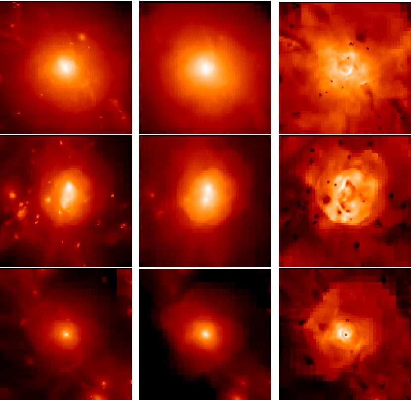
Figure 10.— Three clusters. Top row appears relaxed, middle row has disturbed morphology and bottom row has a cool core. Left column shows X-ray surface brightness from simulated cluster, middle column is Compton $y$ parameter and right column is emission weighted temperature. Images are $\sim 5h^{-1}Mpc$ on a side.

Table 6Gas Mass Estimates for Three Clusters

State	X-ray $M_{est}/M_{true}$	SZE $M_{est}/M_{true}$	$M_{tot}$ ($M_{\odot}$)
Relaxed	1.00	0.94	$1.5\times 10^{15}$
Disturbed	1.54	1.07	$5.3\times 10^{14}$
Cooling	1.39	1.10	$1.4\times 10^{14}$

4.4.2 The Problem with Weighing Cool Core Clusters

Though it is clear the SZE is less affected than the X-ray when calculating gas mass for the cool core clusters in the simulation, it is still not obvious why there should be a bias at all. A look at the cluster projected radial profiles helps to illustrate the difference between cool core and non-cool core clusters. Figure 11 shows images of X-ray surface brightness, and radial profiles of X-ray surface brightness, SZE, and projected emission-weighted temperature of the same cluster from two different simulations. One was run with only adiabatic physics and the other with radiative cooling turned on, otherwise the simulations are identical. Where the Compton y-parameter profiles are nearly identical outside the cool core ($\sim 200\;kpc$), the X-ray surface brightness profiles are significantly different. In the adiabatic sample, the surface brightness has a well defined core, and the slope breaks outside of the core. In the cool core case, the radial X-ray surface brightness profile has a very different appearance. Fitting a $\beta$-model to this profile overestimates the density profile, and hence the mass. It is apparent that the result of radiative cooling in the simulation is to impact the cluster in regions outside the cool core as well as inside. Whether heating effects in real clusters will offset such deviations remains to be seen.

For a more direct comparison, Figure 12 shows the radial temperature and surface brightness profiles of two nearly equal mass clusters from the SFF simulation volume. The main difference is that one has a cool core at z=0, and one does not. It is obvious that the cool core extends to roughly 200 kpc in this cluster as well as the one in Figure 11. The profiles of surface brightness are quite different, the non-cool core (NCC) cluster (solid line) has a profile shape well approximated by a $\beta$-model, while the cool core (CC) cluster clearly does not. Table 7 shows the results of fitting a $\beta$-model to each of two projections of each of these clusters. For the NCC cluster, we get close to the correct gas mass, the numbers are slightly high, consistent with the full sample of X-ray clusters. The CC cluster has significantly biased gas mass estimates, a result of the $\beta$-model fit to the profile. Several indications exist identifying the $\beta$-model fitting as the problem, one of which was illustrated earlier in Figure 9. The bias in gas mass estimates for UTP deprojection models is slightly higher than for the full sample of clusters, the bias is much larger for the isothermal $\beta$-model fits. In fact for the clusters in Table 7, the UTP X-ray method overestimates a gas mass only by about 20%.

A first indication of differences is that CC clusters fit to systematically lower values of the core radius than do NCC clusters, and for the CC clusters, the small core radius fit correlates to higher mass overestimates. Table 8 shows the comparison of median fitted values for $\beta$-model parameters for all clusters at z=0, separated into CC and NCC samples. Figure 13 shows the correlation between the ratio of estimated to true mass for the clusters plotted against the value of the fitted core radius. There is a wide distribution of core radii for NCC clusters, but fitting CC clusters typically results in small core radius values. There appears to also be some correlation between smaller core radii and larger mass overestimates for CC clusters. These effects are indications that fitting the $\beta$-model to a CC cluster’s surface brightness profile is problematic. It is clear that the shape of the surface brightness profile is significantly different in CC clusters than in NCC clusters.

For the two clusters whose profiles are shown in Figure 12, we show the comparison of the $\beta$-model fits in Figure 14. The top panels are for the fit to the X-ray surface brightness in each case, where the CC cluster fit applies to the region outside the cool core. While both models (solid line) appear to fit the data fairly well in the radius regime of interest, the lower panels address the true problem. The $\beta$-models which correspond to the upper panels are shown compared to the true density profile of each cluster. For the NCC case, the model is a good fit, leading to a good mass estimate for the cluster. In the CC case, the model strongly overestimates the density profile, leading the the overestimate in mass. This effect is very typical in cool core clusters in our sample. Clearly there is a breakdown in the assumptions of the $\beta$-model for cool core clusters. The physical reasons for this discrepancy are not obvious, and are likely complicated. One expects, however, that if there is more gas contributing to the surface brightness with temperatures below the assumed isothermal temperature in CC clusters that may lead to overestimates in the density. This explanation may help explain the bias in UTP method gas mass estimates. It is clear that directly deprojecting the X-ray and SZE emission from CC clusters also results in somewhat biased estimates. We plan further investigations of cool core clusters in future studies.

Table 7Comparison of Equal Mass Clusters, SFF

Cluster	Proj	$M_{est}/M_{true}$	$r_{c}$ (Mpc)	$\beta$	True $M_{tot}$ ($M_{\odot}$)
CC	1	2.46	0.084	0.70	$1.91\times 10^{14}$
CC	2	2.87	0.071	0.69	$1.91\times 10^{14}$
NCC	1	1.16	0.17	0.93	$1.94\times 10^{14}$
NCC	2	1.08	0.15	0.92	$1.94\times 10^{14}$

Table 8Comparison of X-ray $\beta$-model Parameters, z=0, $r_{500}$

Cluster Sample	$\langle S_{X0}\rangle$	$\langle r_{c}\rangle$	$\langle\beta\rangle$
CC	$4.42\times 10^{10}$	0.12	0.77
Non Cool Core	$1.41\times 10^{10}$	0.18	0.80

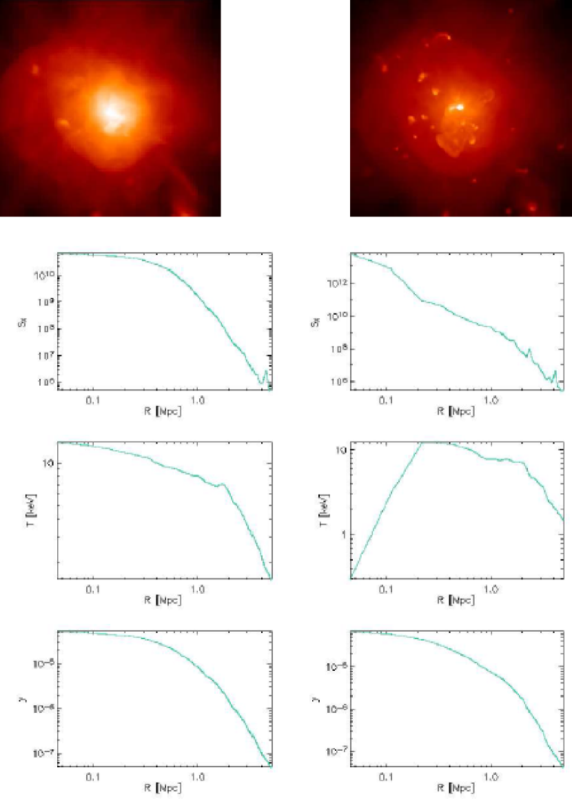
Figure 11.— Same cluster from different cluster catalogs. Left column is from adiabatic physics only simulation, right column is from catalog run with addition of radiative cooling. Top row are images of X-ray surface brightness, second row are X-ray surface brightness radial profiles, third row are radial profiles of projected emission-weighted temperature, bottom row are radial Compton $y$ parameter profiles. Images are $\sim 5h^{-1}Mpc$ on a side.

In cases where the gas is strongly cooled, or has disturbed morphology, the X-ray gas mass determinations are more strongly overestimated. While SZE methods show bias for individual clusters, it is generally smaller than for the X-ray methods. The stronger density dependence of the X-ray emission, and its resultant boosting from density enhancements from cooling, mergers and substructure apparently is responsible for the bias persisting even using profiles to large radii. Any effects which enhance density in localized areas of the cluster will tend to cause overestimates in the cluster total gas mass when using X-ray methods. We expect that X-ray methods of mass estimation for cluster gas will result in a slight bias (5-10%).

4.5. Prospects for Cluster High Resolution SZE Observations

A growing number of SZE telescopes either are active now, or are expected to come online in the next few years. The largest of the single dish instruments capable of resolving radial SZE profiles for many clusters, will be the Large Millimeter Telescope (LMT). Cluster radial SZE profiles will also be generated with the Atacama Large Millimeter Array (ALMA) in a few years time. With ALMA and the LMT, we expect to be able to measure cluster SZE profiles to relatively large radii. In that case, gas mass estimation using SZE profiles can be done to fairly high accuracy. Cluster X-ray profiles are available for many clusters out to $r_{500}$ with XMM-Newton and Chandra imaging. We expect the LMT to observe cluster profiles to similar or larger radii.

In order to estimate the expected cluster radial coverage for the LMT using the Astronomical Thermal Emission Camera (AzTEC) bolometer array, we use the minimum detectable flux density calculation from Pacholczyk (1970)

$$F_{min}=\frac{\sqrt{2}k_{B}T_{sys}}{A_{d}\sqrt{t\Delta\nu}},$$ (12)

where $T_{sys}=54K$, and $\Delta\nu=42\;GHz$ is an estimate for the AzTEC band centered at 144 GHz, and $A_{d}=\pi(50/2)^{2}m^{2}$. This gives a minimum detectable flux density for the LMT of

$$F_{min}=0.26\frac{1}{\sqrt{t}}\;mJy.$$ (13)

To calculate the flux density at $r_{500}$ and $r_{200}$ for simulated clusters, we determine that the typical radial profile average value for clusters of $y(r_{500})\approx 10^{-8}$ and $y(r_{200})\approx 10^{-9}$. Calculating the change in intensity of the CMB at 144 GHz, we estimate

$$\Delta S_{r_{500}}=2.53\times 10^{-7}\;mJy/arcsec^{2}.$$ (14)

The value at $r_{200}$ then is a factor of 10 lower. At $r_{500}(\approx 1h^{-1}Mpc)$ set at z=0.1 in a ring $10\arcsec$ wide, the total flux density from that ring will be F = $12.5\mu Jy$. For $r_{200}(\approx 1.5h^{-1}Mpc)$ at z=0.1, the flux density is F = $1.87\mu Jy$. To observe these with the LMT would require $t\approx 433s$ and $t\approx 72$ minutes per pointing, respectively. These times are very short compared to a typical, high quality, X-ray observation of $t\approx 50ks\approx 14hours$. While this estimate is probably generous, considering the difficulties of atmospheric subtraction and the removal of other instrumental effects, observation of cluster SZE signal out to $r_{200}$ appears to be possible with the LMT.

Table 9Rating of Mass Estimates with Cleaned Samples

Method	Model	Radius	Median	Mean	+1$\sigma$	-1$\sigma$
Xray	UTP	$r_{500}$	1.06	1.07	1.12	1.04
Xray	Iso	$r_{500}$	1.08	1.08	1.13	1.04
SZE	UTP	$r_{200}$	0.98	0.99	1.04	0.94
Joint	Geometric	$r_{500}$	1.09	1.09	1.15	1.04
SZE	y-M	$r_{500}$	0.96	0.98	1.09	0.92
SZE	UTP	$r_{500}$	1.01	1.01	1.09	0.90
SZE	Iso	$r_{500}$	1.08	1.07	1.17	0.99
Xray	$T_{X}$-M	$r_{500}$	1.03	1.01	1.24	0.79

SZE with UTP methods out to large cluster radius produce high precision mass estimates, even without filtering the sample for merging or disturbed clusters. Therefore, from a standpoint of accuracy and simplicity, SZE methods appear to be excellent tools to generate reliable cluster mass measurements to enable precision cosmology with clusters of galaxies.

Figure 12.— Top: Emission weighted projected temperature radial profiles for two clusters of nearly equal mass at z=0 in the SFF sample. Solid line is for a cluster without a cool core, dashed is a cluster with a cool core. Bottom: Surface brightness profiles of same two clusters.

Figure 13.— Ratio of estimated to true gas mass of clusters plotted against fitted value of the $\beta$-model core radius for the SFF sample of clusters at z=0 with a fitting radius of $r_{500}$. Cool core clusters are represented by triangles. Cool core clusters show consistent overestimates in gas mass from X-ray fitting and the magnitude of the overestimate is correlated to the size of the core radius.

Figure 14.— Top Left: X-ray surface brightness profile for non-cool core cluster (NCC) described in text overlaid with best fit $\beta$-model. Top right: X-ray surface brightness profile and best fit model for cool core cluster. Bottom left: True gas density profile of the non-cool core cluster in above panel, again overlaid with best fit $\beta$-model from the surface brightness. Bottom right: same as bottom left, but for cool core cluster whose surface brightness is shown in above panel.

5. Conclusions

The highest precision to which cluster gas masses can be measured using typical assumptions and either X-ray, SZE or a combination of both measurements is $\sim 10$% to $1\sigma$ confidence. This study does not include instrumental or other observational effects, and so is an indication of the limiting ability of observations to correctly gauge the mass of clusters in the ideal case. Our study suggests that when using X-ray observations in a fixed band the scatter is likely higher by a factor of 2-3. These limits in precision are a direct result of the deviation of the simulated clusters from simple assumptions about their physical and thermodynamic properties, dynamical state, and sphericity. To summarize our results, we include Table 9, which shows the relative error for the best cluster gas mass methods compared to one another in order of limiting accuracy. Table 9 also includes scatter estimates for SZE out to $r_{200}$, as well as scatter in total mass estimates using cleaned samples for $y_{500}$ versus mass and the cluster $T_{X}-M$ relation as calculated in Motl et al. (2005).

SZE methods of gas mass estimation assuming a universal temperature profile in the cluster gas produce the smallest scatter when estimating masses in a raw sample of clusters. Cleaning the cluster sample for disturbed or merging clusters is much less important in SZE methods, particularly when profiles can be observed to large radius. As a practical matter, SZE methods are superior for mass estimation for large samples of clusters out to high redshift. This is consistent with previous work, which shows that cluster SZE observations to large cluster radius smooth out boosting effects in the cluster core, and therefore is more representative of the true cluster potential than the X-ray emission.

X-ray mass estimation methods using radial profile fitting do slightly better than SZE methods as far as relative scatter when using a sample cleaned of obvious mergers and disturbed morphology clusters. However, X-ray methods show a 5-10% bias in median values which is absent is SZE methods. The bias is a result of substructure and mergers in clusters, events which enhance the gas density locally. The stronger density dependence of X-ray emissivity tends to drive up the X-ray mass estimates more than the SZE estimates.

Mass estimates fitting radial profiles to a universal temperature profile (UTP) have smaller scatter than similar estimates assuming isothermality, particularly for SZE methods. Also, the accuracy of X-ray mass estimates improves only marginally by increasing the available radius of the observational profiles. This effect can be explained by the strong dependence of the X-ray emission on density, thus on the properties of the cluster core. SZE methods however improve dramatically with profile data out to higher radii, provided one uses a UTP and does not assume the cluster to be isothermal. This is expected since UTP models are a better fit to the real temperature distribution in clusters than isothermal models, and the SZE depends more strongly on temperature than does the X-ray emission.

While the scatter in these estimates varies from method to method, in principle this could be overcome by using a large cluster sample. However, the bias can not be removed in this way. Conveniently, the very small variation in gas mass estimate bias when varying baryonic physics in the simulation suggests that one can use the simulations to correct the bias in observationally determined gas masses. In all but the most extreme case (radiative cooling only) of our samples, the bias in X-ray estimated gas masses is about 7-9%. The bias is also the same (9%) when using a soft (0.5-2.0keV) band and spectroscopic-like temperature to estimate masses. This indicates that the bias is relatively robust, and can be corrected.

Cool core clusters in our catalogs are particularly poor candidates for precision mass estimation in disagreement with previous assumptions. Even when excising the cool core from the analysis, mass estimation shows larger scatter in both X-ray and SZE methods than for non-cool core clusters. X-ray methods also generate a very high ($\sim 50-100\%$) bias in the median value of the cluster gas mass. The proximate cause of bias in cool core clusters is the poor fit of the $\beta$-model from the X-ray surface brightness profiles to the cluster’s true gas density profile. The shape of the surface brightness profile in cool core clusters is markedly different from the profile in non-cool core clusters, and is similar throughout the cool core samples of clusters. This results in $\beta$-model parameters which have systematically small values of the core radius, and large central surface brightness values. When using UTP deprojection methods, the bias and scatter in cool core cluster gas mass estimates is greatly reduced. This remaining bias may also be due to a larger amount of cooler gas contributing to the X-ray surface brightness. This difference in cool gas content is possibly related to differences in merging history between CC and NCC clusters.

In order for this study to provide direct guidance to observers, it remains to include instrumental effects. To truly gauge the likely accuracy of gas mass estimates, we need to examine these effects in detail by simulating the instrumentation and background. Additionally, it is important to examine the systematic errors generated when computing cluster total masses from either the assumption of hydrostatic equilibrium in the cluster, or from lensing data. This is left to future work.

References

- Allen (1998) Allen, S. W. 1998, MNRAS, 296, 392
- Bialek et al. (2001) Bialek, J. J., Evrard, A. E., & Mohr, J. J. 2001, ApJ, 555, 597
- Brickhouse et al. (1995) Brickhouse, N. S., Raymond, J. C., & Smith, B. W. 1995, ApJS, 97, 551
- Buote (2000) Buote, D. A. 2000, ApJ, 539, 172
- Cavaliere & Fusco-Femiano (1978) Cavaliere, A. & Fusco-Femiano, R. 1978, A&A, 70, 677
- Cavaliere et al. (1998) Cavaliere, A., Menci, N., & Tozzi, P. 1998, ApJ, 501, 493
- Cen & Ostriker (1992) Cen, R. & Ostriker, J. P. 1992, ApJ, 399, L113
- Evrard et al. (1996) Evrard, A. E., Metzler, C. A., & Navarro, J. F. 1996, ApJ, 469, 494
- Fabian et al. (1981) Fabian, A. C., Hu, E. M., Cowie, L. L., & Grindlay, J. 1981, ApJ, 248, 47
- Finoguenov et al. (2001) Finoguenov, A., Reiprich, T. H., & Böhringer, H. 2001, A&A, 368, 749
- Haiman et al. (2001) Haiman, Z., Mohr, J. J., & Holder, G. P. 2001, ApJ, 553, 545
- King (1966) King, I. R. 1966, AJ, 71, 64
- King (1972) —. 1972, ApJ, 174, L123+
- Kriss et al. (1983) Kriss, G. A., Cioffi, D. F., & Canizares, C. R. 1983, ApJ, 272, 439
- Loken et al. (2002) Loken, C., Norman, M. L., Nelson, E., Burns, J., Bryan, G. L., & Motl, P. 2002, ApJ, 579, 571
- Mathiesen et al. (1999) Mathiesen, B., Evrard, A. E., & Mohr, J. J. 1999, ApJ, 520, L21
- Mohr et al. (1999) Mohr, J. J., Mathiesen, B., & Evrard, A. E. 1999, ApJ, 517, 627
- Motl et al. (2004) Motl, P. M., Burns, J. O., Loken, C., Norman, M. L., & Bryan, G. 2004, ApJ, 606, 635
- Motl et al. (2005) Motl, P. M., Hallman, E. J., Burns, J. O., & Norman, M. L. 2005, ApJ, 623, L63
- O’Hara et al. (2006) O’Hara, T. B., Mohr, J. J., Bialek, J. J., & Evrard, A. E. 2006, ApJ, 639, 64
- O’Shea et al. (2005) O’Shea, B. W., Bryan, G., Bordner, J., Norman, M. L., Abel, T., Harkness, R., & Kritsuk, A. 2005, in Adaptive Mesh Refinement: Theory and Applications (Berlin: Springer), 341
- Pacholczyk (1970) Pacholczyk, A. G. 1970, Radio astrophysics. Nonthermal processes in galactic and extragalactic sources (Series of Books in Astronomy and Astrophysics, San Francisco: Freeman, 1970)
- Patel et al. (2000) Patel, S. K., Joy, M., Carlstrom, J. E., Holder, G. P., Reese, E. D., Gomez, P. L., Hughes, J. P., Grego, L., & Holzapfel, W. L. 2000, ApJ, 541, 37
- Pen (1997) Pen, U. 1997, New Astronomy, 2, 309
- Rasia et al. (2006) Rasia, E., Ettori, S., Moscardini, L., Mazzotta, P., Borgani, S., Dolag, K., Tormen, G., Cheng, L. M., & Diaferio, A. 2006, ArXiv, astro-ph/0602434
- Rasia et al. (2005) Rasia, E., Mazzotta, P., Borgani, S., Moscardini, L., Dolag, K., Tormen, G., Diaferio, A., & Murante, G. 2005, ApJ, 618, L1
- Ricker & Sarazin (2001) Ricker, P. M. & Sarazin, C. L. 2001, ApJ, 561, 621
- Rines et al. (1999) Rines, K., Forman, W., Pen, U., Jones, C., & Burg, R. 1999, ApJ, 517, 70
- Roettiger et al. (1996) Roettiger, K., Burns, J. O., & Loken, C. 1996, ApJ, 473, 651
- Sanderson et al. (2003) Sanderson, A. J. R., Ponman, T. J., Finoguenov, A., Lloyd-Davies, E. J., & Markevitch, M. 2003, MNRAS, 340, 989
- Sasaki (1996) Sasaki, S. 1996, PASJ, 48, L119
- Shimizu et al. (2003) Shimizu, M., Kitayama, T., Sasaki, S., & Suto, Y. 2003, ApJ, 590, 197
- Sunyaev & Zeldovich (1972) Sunyaev, R. A. & Zeldovich, Y. B. 1972, Comments on Astrophysics and Space Physics, 4, 173
- Vikhlinin et al. (1999) Vikhlinin, A., Forman, W., & Jones, C. 1999, ApJ, 525, 47
- Vikhlinin et al. (2006) Vikhlinin, A., Kravtsov, A., Forman, W., Jones, C., Markevitch, M., Murray, S. S., & Van Speybroeck, L. 2006, ApJ, 640, 691
- Vikhlinin et al. (2005) Vikhlinin, A., Markevitch, M., Murray, S. S., Jones, C., Forman, W., & Van Speybroeck, L. 2005, ApJ, 628, 655
- Voit et al. (2002) Voit, G. M., Bryan, G. L., Balogh, M. L., & Bower, R. G. 2002, ApJ, 576, 601