Gravitational Waves from Phase-Transition Induced Collapse of Neutron Stars

Abstract

We study the gravitational radiation from gravitational collapses of rapidly rotating neutron stars induced by a phase transition from normal nuclear matter to a mixed phase of quark and nuclear matter in the core of the stars. The study is based on self-consistent three-dimensional hydrodynamic simulations with Newtonian gravity and a high-resolution shock-capturing scheme and the quadrupole formula of gravitational radiation. The quark matter of the mixed phase is described by the MIT bag model and the normal nuclear matter is described by an ideal fluid EOS. While there is a broad range of interesting astrophysics problems associated with the phase-transition-induced gravitational collapse, we focus on the following: First, we determine the magnitudes of the emitted gravitational waves for several collapse scenarios, with gravitational wave amplitudes ranging from $0.3\times 10^{-22}$ to $1.5\times 10^{-22}$ for a source distance of 10 Mpc and the energy being carried away by the gravitational waves ranging between $0.3\times 10^{51}$ and $2.8\times 10^{51}\ {\rm ergs}$. Second, we determine the types and frequencies of the fluid oscillation modes excited by the process. In particular, we find that the gravitational wave signals produced by the collapses are dominated by the fundamental quadrupole and quasi-radial modes of the final equilibrium configurations. The two types of modes have comparable amplitude, with the latter mode representing the coupling between the rotation and radial oscillations induced by the collapse. In some collapse scenarios, we find that the oscillations are damped out within a few dynamical timescales due to the growth of differential rotations and the formation of strong shock waves. Third, we show that the spectrum of the gravitational wave signals is sensitive to the EOS, implying that the detection of such gravitational waves could provide useful constraints on the EOS of newly born quark stars. Finally, for the range of rotation periods studied, we find no sign of the development of nonaxisymmetric dynamical instabilities in the collapse process.

1 Introduction

When nuclear matter is squeezed to a sufficiently high density, it turns into uniform two-flavor quark matter ($u$ and $d$) and subsequently to three-flavor ($u$, $d$, and $s$) strange quark matter (SQM), since it is expected that SQM may be more stable than nuclear matter (Bodmer, 1971; Witten, 1984). Up to now there is still no definitive conclusion on the exact conditions for the phase transition to occur. But it is reasonable to assume that deconfined quark matter appears when the density is so high that the nucleons are “touching” each other. At this point, where the number density of nucleons $n\sim 0(1\ {\rm fm}^{-3})$, the quarks lose their correlation with individual nucleons and appear in a deconfined phase. Since the density required for this to happen is not much higher than nuclear matter density ($0.16\ {\rm fm}^{-3}$), the dense cores of neutron stars are the most likely places where the phase transition to quark matter may occur astrophysically. It should be noted that strange quarks (in a confined phase) could already exist in neutron stars with a hyperon core.

If SQM is absolutely stable, then once an SQM seed is formed inside the core of a neutron star, it will begin to swallow the nuclear matter in its surroundings. The SQM region will grow, and the neutron star will become a strange star consisting only of deconfined quarks. In principle, the existence of a thin crust of normal matter is possible at the surface of a strange star. On the other hand, if SQM is metastable at zero pressure, so that it is relatively more stable than nuclear matter only because of the high pressure in the cores of neutron stars, then the final products of the phase transition would be hybrid stars, which consist of quark matter cores surrounded by normal matter outer parts. In this case, the quark matter cores can be either in a pure quark matter phase or a mixed phase of quark and hadronic matter (see, e.g., Glendenning (2002); Madsen (1999) for reviews). In this paper, we do not distinguish between the two different scenarios, and we simply call the final product of the phase transition a quark star.

Since it was first realized that quark stars may exist in nature, much efforts has been put into their study. For example, the possibility that the conversion of neutron stars into strange stars might power cosmological $\gamma$-ray bursts has been considered (see, e.g., Cheng & Dai (1996); Ma & Xie (1996); Bombaci & Datta (2000)). Because the equation of state (EOS) describing the SQM is “softer” than that of the nuclear matter, quarks stars are in general more compact than neutron stars. The phase transition softens the EOS and leads to a collapse, and the conversion process liberates a huge amount of binding energy, on the order of $10^{52}$ ergs, which is required to power a $\gamma$-ray burst. Recently, the formation of quark stars has been invoked to explain the apparent bi modality of Type Ic supernovae (Paczyński & Haensel, 2005). The prospect of detecting the gravitational wave signals emitted by quark stars has also been considered (e.g., Cheng & Dai (1998); Andersson et al. (2002); Marranghello et al. (2002); Gondek-Rosinska et al. (2003); Oechslin et al. (2004); Limousin et al. (2005); Yasutake et al. (2005)).

On the observational side, it has recently been suggested that the compact X-ray source RXJ1856 is a quark star (Drake et al., 2002). But the evidence is not yet conclusive. In fact, recent results suggest that RXJ1856 is more likely to be a neutron star endowed with a strong magnetic field (Thoma et al., 2004). The observational difficulty in distinguishing quark stars (if they exist) from neutron stars arises from the fact that gravity dominates over the strong interaction for compact objects with masses larger than $\sim 1.4M_{\odot}$. This in turn implies that there is no significant difference between the radii of neutron stars and quark stars.

One possible situation in which such phase-transition-induced collapses can occur is accreting neutron stars in low-mass $X$-ray binaries (LMXBs). Neutron stars in these systems are spun up by accreting matter from their lower mass companions. The neutron stars can accrete a mass $\gtrsim 0.5M_{\odot}$ in a timescale of $\sim 10^{8}$ yr and become relatively massive millisecond pulsars. The density in the cores of these neutron stars may be high enough for the nuclear matter to undergo phase transition. It has been suggested (Cheng & Dai, 1998) that the gravitational wave signals emitted from the phase-transition induced collapse of neutron stars in these systems may be detectable by advanced gravitational wave detectors such as LIGO II.

While an initial estimate by Olinto (1987) suggested that the conversion of neutron stars into quark stars should proceed in a slow mode, later investigations by Horvath & Benvenuto (1988) and Lugones et al. (1994) pointed out that the conversion may in fact proceed at a much faster pace in a detonation mode, with the process being completed in a timescale about 0.1 ms. Nevertheless, it is important to stress that at the moment there is still no definitive conclusion on the timescale of this conversion process.

In this paper, we take the first step to investigate the dynamics of phase-transition-induced collapses by performing three-dimensional numerical simulations in Newtonian hydrodynamics and gravity. In particular, we study the gravitational wave signals emitted during the collapse of rotating neutron stars. We assume that (1) initially an SQM seed is formed inside the core of a neutron star, (2) the conversion process is completed within a timescale much shorter than the dynamical timescale of the star, and (3) the result of the conversion is a quark star with a mixed phase of nuclear and quark matter inside the high density core surrounded by a normal nuclear matter region that extends to the star’s surface.

Our initial stellar model before the phase transition is a uniformly rotating equilibrium neutron star modeled by a polytropic EOS $P=k\rho^{\Gamma_{0}}$. The collapse is induced by changing the polytropic EOS to a “softer” EOS for the mixed phase of quark and nuclear matter throughout the star initially. The star undergoes a gravitational collapse due to the reduction of the pressure. When the core of the star reaches a high enough density, the pressure gradient becomes large enough to balance the gravitational force and the star bounces back and oscillates. Due to the coupling between the star’s rotation and oscillations, the quadrupole mass moment of the star changes rapidly leading to strong gravitational radiations.

The main focus of this paper is to study the features of the gravitational wave signals emitted from this kind of phase-transition-induced collapse of neutron stars. Our simulations suggest that the gravitational wave signals are dominated by the fundamental quasi-radial and quadrupole modes of the final equilibrium stars. While the frequencies of the fluid modes depend sensitively on the EOS model of the resulting quark stars, which is not yet established, we find that the excitation of these two fluid modes is quite general and does not depend much on the EOS model. The detection of such gravitational wave signals would provide important information about the EOS of quark matter. For the range of rotation periods we studied, we found no sign of development of nonaxisymmetric dynamical instabilities in the collapse process. For the collapse models considered in this paper, we find that the gravitational wave signals have frequencies of $\sim 2-3$ kHz and amplitudes of $\sim 10^{-22}$ for sources located 10 Mpc away, and the energy carried away by the gravitational waves ranges from $0.27\times 10^{51}$ to $2.76\times 10^{51}\ {\rm ergs}$.

The plan of this paper is as follows: In Sec. 2 we outline the Newtonian hydrodynamics equations and the finite differencing scheme used in the numerical simulations. We also describe the numerical quadrupole formalism for the extraction of gravitational wave signals. Sec. 3 describes the EOS models used in this paper. In Sec. 4 we present the numerical results. Finally, we summarize and discuss our results in Sec. 5.

2 Newtonian Hydrodynamics Equations

In this section, we present the system of Newtonian hydrodynamics equations for a non-viscous fluid flow and the numerical method that we use in the simulations. We also describe the numerical quadrupole formalism for the extraction of gravitational wave signals. Various consistency and convergence tests have been done to validate our numerical code. This includes the “standard” Riemann shock tubes, static and boosted neutron stars, and binary neutron stars in orbit (Gressman et al., 1999). Recently, we have also demonstrated the capability of our code to evolve a rapidly rotating neutron star accurately for long-term simulation (Gressman et al., 2002; Lin & Suen, 2004).

2.1 Equations

The system of equations describing the non viscous Newtonian fluid flow is given by

$$\frac{\partial\rho}{\partial t}+\nabla\cdot\left(\rho{\bf v}\right)=0,$$ (1)

$$\frac{\partial}{\partial t}\left(\rho v_{i}\right)+\nabla\cdot\left(\rho v_{i}{\bf v}\right)+\frac{\partial P}{\partial x_{i}}=-\rho\frac{\partial\Phi}{\partial x_{i}},$$ (2)

$$\frac{\partial\tau}{\partial t}+\nabla\cdot\left(\left(\tau+P\right){\bf v}\right)=-\rho{\bf v}\cdot\nabla\Phi,$$ (3)

where $\rho$ is the mass density of the fluid, ${\bf v}$ is the velocity with Cartesian components $v_{i}$ ($i=1,2,3$), $P$ is the fluid pressure, $\Phi$ is the Newtonian potential, and $\tau$ is the total energy density, defined by

$$\tau=\rho\epsilon+\frac{1}{2}\rho{\bf v}^{2},$$ (4)

in which $\epsilon$ is the internal energy per unit mass of the fluid. The Newtonian potential $\Phi$ is determined by

$${\nabla}^{2}\Phi=4\pi G\rho.$$ (5)

The system is completed by specifying an EOS $P=P(\rho,\epsilon)$.

The system of equations (1)-(3) represents a hyperbolic system of first-order, flux-conservative equations in the form of:

$$\frac{\partial}{\partial t}\vec{U}+\nabla\cdot\vec{F}=\vec{S}.$$ (6)

The evolved variables $\vec{U}$, the fluxes $\vec{F^{j}}$ and the sources $\vec{S}$ are given by

$$\vec{U}=\left[\begin{array}[]{c}\rho\\ \rho v_{i}\\ \rho\epsilon+\frac{1}{2}\rho{\bf v}^{2}\end{array}\right],$$ (7)

$$\vec{{F}^{j}}=\left[\begin{array}[]{c}\rho v_{j}\\ \rho v_{i}v_{j}+P\delta^{j}_{i}\\ \left(\rho\epsilon+\frac{1}{2}\rho{\bf v}^{2}+P\right)v_{j}\end{array}\right],$$ (8)

$$\vec{S}=\left[\begin{array}[]{c}0\\ -\rho\frac{\partial\Phi}{\partial x_{i}}\\ -\rho{\bf v}\cdot\nabla\Phi\end{array}\right].$$ (9)

In each vector above, $i$ ranges from 1 to 3 (for $x$, $y$, and $z$), thus making the vector five-dimensional. Also note that in the case of $\vec{F^{j}}$, $j$ goes from 1 to 3, so that we have a total of five vectors, each with five components.

2.2 Spectral Decomposition of the Characteristic Matrix

Our Newtonian hydrodynamics code uses a high resolution shock capturing (HRSC) scheme (Hirsch, 1992) to solve Eq. (6). A HRSC scheme, using either exact or approximate Riemann solvers, with the characteristic fields (eigenvalues) of the system, has the ability to resolve discontinuities in the solution (e.g., shock waves). Moreover, such schemes have high accuracy in regions where the fluid flow is smooth.

To implement the HRSC schemes, it is necessary to decompose the characteristic matrix of the system, $\frac{\partial\vec{F^{j}}}{\partial\vec{U}}$, to determine the characteristic fields (eigenvectors) and the characteristic speeds of those fields (the corresponding eigenvalues). For any EOS in which the pressure $P$ is a function of $\rho$ and $\epsilon$, the speed of sound in the fluid $c_{s}$ is given by

$$c_{s}^{2}={\left.\frac{\partial P}{\partial\rho}\right|}_{\cal S}={\left.\frac{\partial P}{\partial\rho}\right|}_{\epsilon}+\frac{P}{\rho^{2}}{\left.\frac{\partial P}{\partial\epsilon}\right|}_{\rho},$$ (10)

where ${\cal S}$ is the entropy per particle. The characteristic matrix possesses a complete set of linearly independent eigenvectors ${\vec{r}}_{i}$ rendering the system strongly hyperbolic. For example, the $x$ component of the flux term, $\vec{F^{x}}$, in Eq. (6), has the characteristic matrix $\frac{\partial\vec{F^{x}}}{\partial\vec{U}}$. Its five eigenvectors satisfy the equation

$$\left[\frac{\partial\vec{F^{x}}}{\partial\vec{U}}\right]\left[{\vec{r}}_{i}\right]={\lambda}_{i}\left[{\vec{r}}_{i}\right]\ ;\ i=1,\cdots,5,$$ (11)

where the eigenvalues $\lambda_{i}$ are given by:

$$\lambda_{1}=\lambda_{2}=\lambda_{3}=v_{x},$$ (12)

$$\lambda_{4}=v_{x}+c_{s},$$ (13)

$$\lambda_{5}=v_{x}-c_{s}.$$ (14)

Explicitly, the five right eigenvectors of the Jacobian are

$$\vec{r}_{1}={\left[1,v_{x},v_{y},v_{z},H-\frac{c_{s}^{2}}{\gamma-1}\right]}^{T},$$ (15)

$$\vec{r}_{2}={\left[0,0,\rho,0,\rho v_{y}\right]}^{T},$$ (16)

$$\vec{r}_{3}={\left[0,0,0,\rho,\rho v_{z}\right]}^{T},$$ (17)

$$\vec{r}_{4}=\frac{\rho}{2c_{s}}{\left[1,v_{x}+c_{s},v_{y},v_{z},H+v_{x}c_{s}\right]}^{T},$$ (18)

$$\vec{r}_{5}=\frac{\rho}{2c_{s}}{\left[1,v_{x}-c_{s},v_{y},v_{z},H-v_{x}c_{s}\right]}^{T},$$ (19)

where the total enthalpy $H=\epsilon+\frac{{\bf v}^{2}}{2}+\frac{P}{\rho}$ is introduced along with $\gamma=1+\frac{1}{\rho}\frac{\partial P}{\partial\epsilon}$. The superscript $T$ denotes transpose. The eigenvalues and eigenvectors for the $y$ and $z$ components can be obtained from a cyclic permutation of spatial indices and components of each $\vec{r}_{i}$.

2.3 Finite Differencing Method

To solve equations (1)-(3) numerically, the system must be suitably discretized in both space and time. In our code we use a discretization scheme that is second-order accurate in time. The spatial order, however, depends on which cell reconstruction method we choose (see below).

We first consider the discretization in space. We show the discretization in the $x$-direction only; the other spatial dimensions are handled in a similar manner. We also consider the equations in the absence of source terms since the discretization of the source terms does not present any difficulties.

The problem, then, is reduced to finding the appropriate update of the state vector $\vec{U}$ for fluxes in the $x$-direction:

$$\frac{\partial\vec{U}}{\partial t}+\frac{\partial\vec{F^{x}}}{\partial x}=0.$$ (20)

The spatial discretization of this equation can be written in the standard manner:

$$\frac{\partial\vec{U}_{i}}{\partial t}+\frac{(\vec{f^{\ast}})_{i+1/2}-(\vec{f^{\ast}})_{i-1/2}}{\Delta x}=0,$$ (21)

where $(\vec{f^{\ast}})_{i\pm 1/2}$ is the “numerical flux” evaluated at the interfaces $i\pm 1/2$ of the spatial cell $i$ using information from the left and right sides. The state variables $\rho$, $\epsilon$, and ${\bf v}$, which are cell-centered quantities, must be properly reconstructed and interpolated to the cell interfaces. This cell-reconstruction procedure controls the spatial order of the numerical scheme. In our implementation, we use the third-order piecewise parabolic method (PPM Collela & Woodward (1984)) for the reconstruction.

To calculate the numerical fluxes, we make use of Roe’s approximate Riemann solver (Roe, 1981). Roe’s solver is well-established and widely used. It has good shock capturing capability and can be used for a wide range of equations of state. For a detailed discussion of the Roe’s scheme, see for example, Hirsch (1992). With the fluid state interpolated to the cell interfaces, the formula for the numerical flux then becomes

$$(\vec{f^{\ast}})_{i+1/2}=\frac{1}{2}\left[\vec{F^{x}_{L}}+\vec{F^{x}_{R}}-\sum_{j=1}^{5}|\tilde{\lambda}_{j}|{\Delta\tilde{\omega}_{j}}\tilde{\vec{r}_{j}}\right].$$ (22)

Here $\vec{F^{x}_{L}}$ and $\vec{F^{x}_{R}}$ are the fluxes computed using, respectively, the primitive variables to the left and right of the interface between the $i$-th and $(i+1)$-th cells. Both $\tilde{\lambda}_{j}$ and $\tilde{\vec{r}_{j}}$ are computed by Eqs. (12)-(19) using the following weighted quantities:

$$\tilde{\rho}=\sqrt{\rho_{i}\rho_{i+1}},$$ (23)

$$\tilde{\bf v}=\frac{({\bf v}\sqrt{\rho})_{i}+({\bf v}\sqrt{\rho})_{i+1}}{\sqrt{\rho_{i}}+\sqrt{\rho_{i+1}}},$$ (24)

$$\tilde{H}=\frac{(H\sqrt{\rho})_{i}+(H\sqrt{\rho})_{i+1}}{\sqrt{\rho_{i}}+\sqrt{\rho_{i+1}}}.$$ (25)

Finally, the quantities $\Delta\tilde{\omega}_{j}$ represent the jumps in the characteristic variables across each characteristic field, and are obtained from

$$\vec{U}_{R}-\vec{U}_{L}=\sum_{j}{\Delta\tilde{\omega}_{j}}\tilde{\vec{r}_{j}}.$$ (26)

Next we turn to temporal discretization. To achieve second-order accuracy in time, we employ a basic two-step method. Given the fluid state at the mesh points $\vec{U}_{i}^{n}$, where $i$ represents the spatial mesh and $n$ represents the time coordinate of the state variables, we calculate $\vec{U}_{i}^{n+1/2}$, the fluid state midway between the time $t$ and $t+\Delta t$, to first order:

$$\frac{\vec{U}_{i}^{n+1/2}-\vec{U}_{i}^{n}}{(\Delta t/2)}+\frac{(\vec{f^{\ast}})_{i+1/2}^{n}-(\vec{f^{\ast}})_{i-1/2}^{n}}{\Delta x}=\vec{S}_{i}^{n}.$$ (27)

Here we have included the source term $\vec{S}_{i}^{n}$. The fluid state $\vec{U}_{i}^{n+1}$ is then given by:

$$\frac{\vec{U}_{i}^{n+1}-\vec{U}_{i}^{n}}{\Delta t}+\frac{(\vec{f^{\ast}})_{i+1/2}^{n+1/2}-(\vec{f^{\ast}})_{i-1/2}^{n+1/2}}{\Delta x}=\vec{S}_{i}^{n+1/2}.$$ (28)

2.4 Generation of gravitational waves

We calculate the gravitational wave signals emitted during a gravitational collapse using the standard quadrupole approximation, which is valid for a nearly Newtonian system (see, e.g., the recent review by Flanagan & Hughes (2005) for details). The power emitted in gravitational waves is given by

$${dE\over dt}={G\over 5c^{5}}{Q}_{ij}^{(3)}{Q}_{ij}^{(3)},$$ (29)

where the superscript (3) indicates the third time derivative and the traceless quadrupole moment of the mass distribution $Q_{ij}$ is defined by

$$Q_{ij}=\int{\rho(x^{i}x^{j}-{1\over 3}\delta^{ij}r^{2})d^{3}x}.$$ (30)

The total energy radiated in the form of gravitational wave is calculated by

$$\Delta E_{\rm GW}(t)=\int_{0}^{t}dt{dE\over dt}.$$ (31)

For simplicity we evaluate the gravitational waveforms on the $x$-axis (where the $z$-axis is the rotation axis). The nonvanishing components of the leading order radiative gravitational field $h_{ij}^{\rm TT}$ are

$$h_{+}\equiv h_{yy}^{\rm TT}=-h_{zz}^{\rm TT}={G\over c^{4}r}\left(\ddot{Q}_{yy}-\ddot{Q}_{zz}\right),$$ (32)

$$h_{\times}\equiv h_{yz}^{\rm TT}={2G\over c^{4}r}\ddot{Q}_{yz}.$$ (33)

where $\ddot{Q}_{ij}$ denotes the second time derivative of $Q_{ij}$. Using direct finite-differencing method to calculate the high-order time derivatives of $Q_{ij}$ in numerical simulation would generate a large amount of unwanted noise. In our simulations, we follow a standard approach to reexpress $\ddot{Q}_{ij}$ as an integral over the fluid variables and calculate them on each time slice (see, e.g., Blanchet et al. (1990); Finn & Evans (1990); Zwerger & Müller (1997)).

We also calculate the gravitational wave signal using the angle-averaged waveforms for the polarization states $h_{+}$ and $h_{\times}$ (Centrella & McMillan, 1993):

$$<(rh_{+})^{2}>={1\over 4\pi}\int(rh_{+})^{2}d\Omega,$$ (34)

$$<(rh_{\times})^{2}>={1\over 4\pi}\int(rh_{\times})^{2}d\Omega,$$ (35)

where $d\Omega$ is a solid angle element. The angle brackets denote averaging over all source orientations. In terms of $\ddot{Q}_{ij}$ they are given explicitly by (Centrella & McMillan, 1993)

$$<(rh_{+})^{2}> = {G\over c^{8}}\left[{4\over 15}(\ddot{Q}_{xx}-\ddot{Q}_{zz})^{2}+{4\over 15}(\ddot{Q}_{yy}-\ddot{Q}_{zz})^{2}+{1\over 10}(\ddot{Q}_{xx}-\ddot{Q}_{yy})^{2}+{14\over 15}(\ddot{Q}_{xy})^{2}\right.$$ (38)

$$\left.+{4\over 15}(\ddot{Q}_{xz})^{2}+{4\over 15}(\ddot{Q}_{yz})^{2}\right],$$

$$<(rh_{\times})^{2}>={G\over c^{8}}\left[{1\over 6}(\ddot{Q}_{xx}-\ddot{Q}_{yy})^{2}+{2\over 3}(\ddot{Q}_{xy})^{2}+{4\over 3}(\ddot{Q}_{xz})^{2}+{4\over 3}(\ddot{Q}_{yz})^{2}\right].$$ (39)

3 Equation of State

3.1 Initial neutron star model

We model our initial equilibrium rotating neutron star before the phase transition by a polytropic EOS

$$P=k_{0}\rho^{\Gamma_{0}},$$ (40)

where $k_{0}$ and $\Gamma_{0}$ are constants. On the initial time slice, we also need to specify the specific internal energy $\epsilon$. For the polytropic EOS, the thermodynamically consistent $\epsilon$ is given by

$$\epsilon={k_{0}\over\Gamma_{0}-1}\rho^{\Gamma_{0}-1}.$$ (41)

Note that the pressure in Eq. (40) can also be written as

$$P=(\Gamma_{0}-1)\rho\epsilon.$$ (42)

3.2 Quark matter

In the literature, the so-called MIT bag model EOS has been used extensively to describe quark matter inside compact stars (see, e.g., Glendenning (2002); Madsen (1999)). In our study, we assume that the quarks are massless. We note that while it is a good approximation to neglect the $u$- and $d$-quark masses, since they are much smaller than the quark chemical potential, which is on the order of 300 MeV, this is not the case for the $s$-quark mass, $m_{s}\sim O(100)$ MeV. Nevertheless, the inclusion of the $s$-quark mass would decrease the pressure by only a few percent (Alcock & Olinto, 1988). Hence, we do not expect that the inclusion of the $s$-quark mass would change our results qualitatively.

Assuming that the quarks are massless, the MIT bag model EOS is given by

$$P={1\over 3}(\rho_{\rm tol}-4B),$$ (43)

where $\rho_{\rm tol}$ is the (rest frame) total energy density and $B$ is the so-called bag constant. The quarks are asymptotically free in the limit $\rho_{\rm tol}\rightarrow\infty$. At finite densities, the quark interactions, and hence the confinement effect must be taken into account. The bag constant $B$ is a phenomenological parameter that describes this confinement. It should be noted that at the moment there is no general consensus on the best value of $B$ to describe quark matter. The result from fits of the hadronic spectrum gives $B^{1/4}\approx 145$ MeV (in units of $\hbar=c=1$) (DeGrand et al., 1975), while the calculation of hadronic structure functions suggests $B^{1/4}\sim 170$ MeV (Steffens et al., 1995). On the other hand, lattice QCD results suggest a value up to $B^{1/4}\sim 190$ MeV (Satz, 1982). Many investigators have used different values of $B$ within the range $B^{1/4}\sim 145-200$ MeV to study quark matter inside neutron stars. In our simulations, we employ the MIT bag model with $B^{1/4}=170$ MeV for the quark matter in the mixed phase EOS described below.

In our Newtonian simulations, we use the rest-mass density $\rho$ and specific internal energy $\epsilon$ as fundamental variables in the hydrodynamics equations. The total energy density $\rho_{\rm tol}$, which includes the rest-mass contribution, is decomposed as (in our code units $G=c=M_{\odot}=1$)

$$\rho_{\rm tol}=\rho+\rho\epsilon.$$ (44)

In terms of our hydrodynamic variables the expression for the MIT bag model becomes

$$P_{\rm q}={1\over 3}\left(\rho+\rho\epsilon-4B\right).$$ (45)

The MIT bag model is a relativistic EOS. One might worry that using this EOS in a Newtonian simulation is somewhat inconsistent. However, it should be noted that the MIT bag model is a microscopic phenomenological model, whereas the Newtonian hydrodynamic equations are used to describe the global structure of the star.

3.3 Mixed Phase

As discussed in the introduction, we assume that once a SQM seed is formed inside the core of a neutron star, the star will transform to a quark star on a timescale much shorter than the dynamical timescale of the neutron star. In this short timescale limit, we do not need to model the complicated and poorly known dynamical process of the conversion itself. Instead, we focus on the collapse process of the star due to the softening of the EOS after the conversion is completed. In our simulations, the collapse is induced by changing the initial polytropic EOS (see Eq. (40)) to a “softer” EOS to describe the quark star in the initial time slice.

The model EOS that we consider for the quark star is composed of two parts: (1) a mixed phase of quark and nuclear matter in the core at a density higher than a certain critical value $\rho_{\rm NM}$; (2) a normal nuclear matter region extending from $\rho=\rho_{\rm NM}$ to the surface of the star. Explicitly, the pressure is given by

$$P=\left\{\begin{array}[]{cc}\alpha P_{\rm q}+(1-\alpha)P_{\rm n}&\ \mbox{for}\ \ \rho>\rho_{\rm NM}\\ \\ P_{\rm n}&\mbox{for}\ \ \rho\leq\rho_{\rm NM},\end{array}\right.$$ (46)

where

$$\alpha=\left\{\begin{array}[]{cc}{(\rho-\rho_{\rm NM})/(\rho_{\rm QM}-\rho_{\rm NM})}&\ \mbox{for}\ \ \rho_{\rm NM}<\rho<\rho_{\rm QM}\\ \\ 1&\mbox{for}\ \ \rho_{\rm QM}<\rho,\end{array}\right.$$ (47)

is defined to be the scale factor of the mixed phase, and where $P_{q}$ is the pressure contribution of the quark matter, while $P_{n}$ is that of the nuclear matter. In Eq. (47), $\rho_{\rm QM}$ is defined to be the critical density above which a pure quark matter phase is energetically favored over the mixed phase.

We take $P_{q}$ to be given by the MIT bag model (see Eq. (45)) with a bag constant $B^{1/4}=170$ MeV. The critical density of the phase transition from nuclear matter to pure quark matter is model dependent; it could range from 4 to $8\rho_{\rm nuc}$ (Cheng & Dai, 1998; Haensel, 2003; Bombaci et al., 2004), where $\rho_{\rm nuc}=2.8\times 10^{14}\ {\rm g\ cm^{-3}}$ is the nuclear density. Cheng & Dai (1996) have argued that the accretion induced phase transition from neutron stars to strange stars in low-mass X-ray binaries could be the origin of $\gamma$-ray bursts. They choose the transition density $\sim 8-9\rho_{\rm nuc}$, so that the phase transition cannot occur until a large amount of mass has been transferred from the lower mass companion to the neutron star; otherwise, there may be too many $\gamma$-ray bursts produced from this mechanism. We choose $\rho_{\rm QM}=9\rho_{\rm nuc}$ in our simulation, which can produce stronger gravitational radiation. Other choices of $\rho_{\rm QM}$ are not ruled out but the gravitational radiation will be relatively weaker. In all cases studied in this paper, the maximum value of $\alpha$ is always less than unity during the time evolutions. Also, we define the transition density from the mixed phase to nuclear matter $\rho_{\rm NM}$ to be at the point where $P_{q}$ vanishes initially. This corresponds to $\rho_{\rm NM}=7.25\times 10^{14}\ {\rm g\ cm^{-3}}=2.6\rho_{\rm nuc}$ for $B^{1/4}=170$ MeV in our study.

For the normal nuclear matter, we use an ideal-fluid model

$$P_{\rm n}=(\Gamma-1)\rho\epsilon,$$ (48)

where $\Gamma$ is the effective adiabatic index. In our mixed-phase EOS model, we allow for the possibility that the nuclear matter EOS can be different from that before the phase transition. This is achieved by using values of $\Gamma$ different from the initial value $\Gamma_{0}$. In particular, we choose $\Gamma<\Gamma_{0}$ in our simulations. It is possible that the nuclear matter may not be stable during the phase transition process, and hence some quark seeds could appear inside the nuclear matter. In the presence of the quark seeds in the nuclear matter, the effective adiabatic index will be reduced. In our simulations, $B$, $\rho_{\rm NM}$, and $\rho_{\rm QM}$ are fixed to be the values given above for all cases studied. We consider $\Gamma$ as the only free parameter of the mixed phase EOS.

4 Numerical Results

4.1 General Considerations

The gravitational collapse of compact stellar objects is one of the most promising sources of gravitational waves for interferometer detectors such as LIGO, VIRGO, GEO600, and TAMA300. In the past decade, numerous multidimensional (two- or three-dimensional) hydrodynamic simulations have been performed to study the gravitational wave signals emitted from some collapse processes. For example, the signals from the rotational core collapse to a proto neutron star have been studied in both Newtonian (e.g., Finn & Evans (1990); Mönchmeyer et al. (1991); Bonazzola & Marck (1993); Zwerger & Müller (1997); Rampp et al. (1998); Fryer et al. (2002)) and general relativistic frameworks (Dimmelmeier et al., 2002; Siebel et al., 2003; Shibata & Sekiguchi, 2004; Dimmelmeier et al., 2005; Shibata & Sekiguchi, 2005). While it is still consistent to use Newtonian dynamics to study the rotational core collapse, as gravity is relatively weak in this process, fully general relativistic simulation is required to study the more extreme scenario: the gravitational collapse of rotating neutron stars to black holes. The gravitational wave signals emitted from such a process were studied 20 years ago by Stark & Piran (1985) in two dimensions, and more recently by Baiotti et al. (2005) in three dimensions.

In this paper, we study the gravitational wave signals emitted from the gravitational collapses of rapidly rotating neutron stars to quark stars. In this collapse scenario, gravity is stronger than that in the rotational core collapse, but still not strong enough to produce a black hole (we will return to this point later). To the best of our knowledge, our work is the first hydrodynamic simulation to study this kind of collapse process and the emitted gravitational wave signals in three dimensions.

Before we present our numerical results for the phase-transition induced collapse models based on the mixed phase EOS discussed in Sec. 3.3, in this section we study the features of the gravitational wave signals emitted from such process using a simplified collapse model. Our simulations suggest that the emitted gravitational wave signals are dominated by two fluid oscillation modes. In particular, we demonstrate that these two modes are the fundamental quasi-radial and quadrupole modes of the final equilibrium star. The excitation of these fluid modes is a general feature that does not depend sensitively on the EOS model.

In this study, we use the same initial neutron star configuration as that of the reference model R in the mixed-phase collapse models (see Sec. 4.2). The neutron star is modeled by a polytropic EOS $P=k\rho^{2}$, with the polytropic constant $k=k_{0}=60$. The collapse is induced by reducing the pressure by using a smaller polytropic constant $k=54$ (i.e., a 10% reduction of the pressure) during the evolution. This simplified collapse model has the advantage that it can produce the general feature of the gravitational waveforms that we see in the mixed-phase model, while remaining simple enough that the fluid oscillation modes of the final equilibrium configuration can be studied in detail.

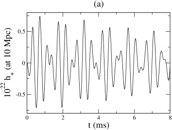
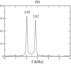
Figure 1: (a) Gravitational waveform $h_{+}$ on the $x$ axis for a simplified collapse model. The initial neutron star is the same as that of the reference model R in Table 1. The neutron star is modeled by a polytropic EOS $P=k\rho^{2}$, with $k=60$. The collapse is induced simply by reducing the value of $k$ by 10%. (b) Fourier transform of $h_{+}$ for the same case.

In Fig. 1 (a) we show the evolution of the gravitational wave amplitude $h_{+}$ on the $x$-axis for this collapse model. For all cases studied in this paper, it is assumed that the source is located at a distance of 10 Mpc (i.e., the distance to nearby galaxies). Our simulations are performed in full three dimensions without any symmetry assumptions. Any non-axisymmetric fluid flow during the evolution can in general produce a nonzero contribution to the wave field $h_{\times}$. Nevertheless, we see that for all models studied in this paper $h_{\times}$ is essentially zero (within numerical accuracy) during the evolution. This suggests that the fluid flow remains axisymmetric during the collapse and no non axisymmetric fluid oscillations are excited. This implies that for the range of rotation periods studied, there are no nonaxisymmetric dynamical instabilities in the collapse process. Hence, we will consider only $h_{+}$ in the rest of this paper.

Fig. 1 (a) shows clearly that the waveform is not dominated by a single oscillation mode. The Fourier transform of $h_{+}$ plotted in Fig. 1 (b) shows that the waveform is composed of two oscillation modes at frequencies 2.03 and 2.82 kHz. To show that these two excited modes are respectively the fundamental quadrupole and quasi-radial modes, we compare the mode frequencies with those obtained by perturbing a configuration that is the same as the final equilibrium star.

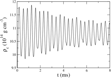
Figure 2: Time evolution of the central density for the simplified collapse model.

To begin, we first need to construct an unperturbed configuration that is the same as the final equilibrium star resulting from the collapse. In Fig. 2 we show the time evolution of the central density $\rho_{\rm c}$. It is seen that $\rho_{\rm c}$ oscillates around its final equilibrium value after the initial collapse phase. However, it is computationally too expensive to run the simulation until the final equilibrium state is reached. Instead, we use the time-average value of $\rho_{\rm c}$ in the period $2-6$ ms, $1.08\times 10^{15}\ {\rm g\ cm^{-3}}$, to approximate the central density of the final equilibrium configuration. To fully specify the configuration, we also need to determine the final spin rate. More generally, we need the profile of the rotational velocity, since differential rotation can develop during the collapse. As we show in Sec. 4.3, for some of the mixed-phase collapse models studied in this paper, the stellar oscillations triggered by the collapse are damped very quickly by the growth of differential rotation. However, it has been shown by Stergioulas et al. (2004) that the frequencies of the quasi-radial and quadrupole modes do not depend sensitively on rotation along a sequence of stellar models with the same central density. Hence, for our purpose, it is accurate enough to study the oscillations of a nonrotating star model that has the same central density as the final equilibrium star produced by the rotational collapse.

The unperturbed nonrotating star is modeled by the polytropic EOS with $k=54$. It has a central density $\rho_{\rm c}=1.08\times 10^{15}\ {\rm g\ cm^{-3}}$, and baryonic mass $M=1.73M_{\odot}$ and radius $R=13.46$ km. To excite a particular mode we add initial perturbation to the equilibrium star. For the fundamental radial ($l=0$) mode, we perturb the velocity by adding a radial perturbation of the form

$$\delta v_{r}=\alpha\sin\left({\pi r\over R}\right),$$ (49)

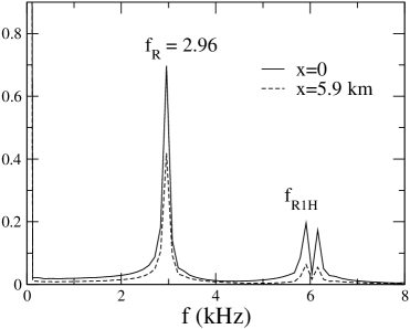
Figure 3: Fourier transforms of the time evolution of the density at $x=0$ and 5.9 km for the radially perturbed nonrotating model discussed in the text. The peaks at $f_{\rm R}$ and $f_{\rm R1H}$ correspond to the fundamental radial mode and its first harmonic respectively.

where $\alpha$ is the amplitude of the perturbation. We use $\alpha=0.03$, which corresponds to 3% of the speed of light. We follow the evolution of the perturbed star using our fully nonlinear evolution code. In Fig. 3 we show the Fourier transforms of the time evolution of the density at $x=0$ and 5.9 km. Fig. 3 shows that the fundamental radial mode at frequency $f_{\rm R}=2.96$ kHz is excited and dominates the time evolution. It is seen that the first harmonic $f_{\rm R1H}$ has also been excited.

For a nonrotating star, the radial mode does not radiate gravitational wave. However, the non radial modifications of the mode eigenfunction due to rotation implies that the radial mode becomes quasi-radial and is capable of emitting gravitational waves (Chau, 1967). We see that the frequency of the fundamental radial mode $f_{\rm R}=2.96$ kHz agrees with the second peak in Fig. 1 (b) to about 5%. This shows that the second peak in Fig. 1 (b), at a frequency of 2.82 kHz, corresponds to the fundamental quasi-radial mode of the final equilibrium star. The fact that the frequencies are so close to one another reinforces the conclusion of Stergioulas et al. (2004), that the frequency of the fundamental quasi-radial mode does not depend sensitively on rotation for a sequence of stellar models with fixed central density.

To excite the fundamental quadrupole mode, we perturb the $\theta$-component of the velocity by (Font et al., 2001; Stergioulas et al., 2004)

$$\delta v_{\theta}=\alpha\sin\left({\pi r\over R}\right)\sin\theta\cos\theta.$$ (50)

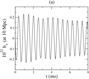
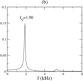
Figure 4: (a) Time evolution of the gravitational wave amplitude $h_{+}$ on the $x$-axis emitted by the quadrupole mode of the nonrotating model discussed in the text. (b) Fourier transform of $h_{+}$ for the same case.

The form of the polar-angle ($\theta$) dependence is motivated by the fact that the $\delta v_{\theta}$ of spheroidal oscillation modes is proportional to $\partial Y_{lm}/\partial\theta$, where $Y_{lm}$ represents the usual spherical harmonics and we want to excite the $l=2$, $m=0$ mode. In Fig. 4 (a) we show the time evolution of the gravitational wave amplitude $h_{+}$ on the $x$ axis. The waveform is dominated only by the excited quadrupole mode. The Fourier transform of $h_{+}$ plotted in Fig. 4 (b) shows that the frequency of the quadrupole mode is $f_{\rm Q}=1.90$ kHz, which agrees with the first peak in Fig. 1 (b) to about 6%. We can thus identify the first peak in Fig. 1 (b) as the fundamental quadrupole mode of the final equilibrium star. Similar to the case of the quasi-radial mode, the difference in the frequencies is due mainly to rotation.

The above results show that the gravitational waveform produced by the simplified collapse model is dominated by two oscillation modes. By studying the oscillations of a nonrotating star model that has the same central density as the final equilibrium star resulting from the collapse, we demonstrated that the two oscillation modes are the fundamental quasi-radial and quadrupole modes of the final star. This conclusion does not depend on the EOS of the collapse model. We have repeated the above simplified collapse model and mode-identification analysis with a different polytropic constant $k=48$ (i.e., a 20% reduction of the initial value $k_{0}=60$) and found that the conclusion still holds. We conclude that the excitation of the fundamental quasi-radial and quadrupole modes is a general feature of the phase-transition-induced collapse of a rapidly rotating neutron star, which does not depend much on the EOS model. In particular, we show that these two modes are excited in all collapse scenarios based on the mixed-phase EOS model.

4.2 Numerical models

In this section, we present the details of the phase-transition induced collapse models based on the mixed phase EOS. To generate initial equilibrium neutron star models for this study, we solve the time-independent hydrodynamics equations using the self-consistent field technique developed by Hachisu (1986). The initial neutron star is uniformly rotating and modeled by a polytropic EOS $P=k_{0}\rho^{\Gamma_{0}}$. We take $\Gamma_{0}=2$ and $k_{0}=60$ in our code units $G=c=M_{\odot}=1$. Unless otherwise noted, we use $129^{3}$ Cartesian grid points with $\Delta x=\Delta y=\Delta z=0.56$ km. We choose the $z$ axis to be the rotation axis in our simulations.

The collapse of the equilibrium neutron star is induced by reducing the pressure via the use of the mixed phase EOS (see Eq. (46)). As discussed in Sec. 3.3, we choose the effective adiabatic index $\Gamma$ as the only free parameter of the mixed phase EOS. We have performed simulations using $\Gamma=1.95$, $1.85$, and $1.75$. Besides the effect of $\Gamma$, we have also compared the gravitational waveforms due to the difference in masses and spin rates of the initial neutron star models. We have performed the seven specific collapse models listed in Table 1. In the table we list the initial central densities $\rho_{\rm c}$, rotation periods $P$, ratios of the rotational kinetic energy to the potential energy $T/|W|$, baryonic masses $M$, equatorial radii $R_{\rm e}$, polar radii $R_{\rm p}$, and the values of $\Gamma$ for the collapse models. Note that we are interested in neutron star models with baryonic masses $\gtrsim 2M_{\odot}$, since it is expected that accreting neutron stars with masses over $2M_{\odot}$ in LMXB are most likely to lead to a phase transition (Cheng & Dai, 1996).

Model R is a reference model to which the other models are compared. The initial neutron star of model R has a (baryonic) mass 2.2 $M_{\odot}$. The rotation period is 1.2 ms. The equatorial radius $R_{\rm e}=17.95$ km. The ratio of the polar to equatorial radii is 0.69. We take $\Gamma=1.85$ for this collapse model. Models G1.95 and G1.75 have the same initial neutron star configuration as that of model R. But their $\Gamma$ values are different. Model G1.95 (G1.75) has a value $\Gamma=1.95\ (1.75)$. On the other hand, models M2.0 and M2.4 have different masses compared to model R. Model M2.0 (M2.4) has a mass 2.0 (2.4) $M_{\odot}$. Finally, models P1.4 and P1.6 have initial rotation period 1.4 and 1.6 ms respectively, with the same baryonic mass 2.2 $M_{\odot}$ as the reference model R.

4.3 Collapse and gravitational waveforms

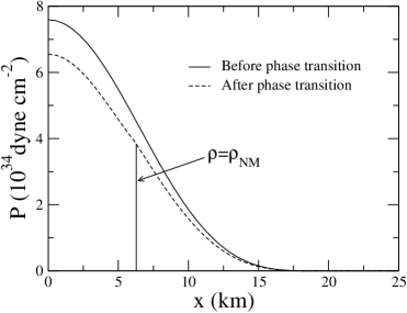
Figure 5: Model R. Pressure profiles along the $x$-axis of the initial neutron star model (solid line) and that immediately after the phase transition (dashed line). The interface between the mixed phase and normal nuclear matter is marked by the vertical line $\rho=\rho_{\rm NM}$.

Fig. 5 shows the pressure profiles along the $x$-axis for the initial neutron star (solid line) and those immediately after the phase transition (dashed line) of the reference model R. The dashed line in Fig. 5 corresponds to the initial state of the pressure profile for the dynamical evolution. Note that the outer boundary of the computational domain is at $x=35.89$ km ($\approx 2R_{\rm e}$) , although we show only up to $x=25$ km in the figure. The interface between the mixed phase and normal nuclear matter is marked by the vertical line $\rho=\rho_{\rm NM}$. Due to the reduction of the pressure after the phase transition, the star undergoes a gravitational collapse. The pressure gradient will balance the gravitational force, halting the collapse, when the core of the star reaches a high enough density. The star subsequently goes into an oscillation phase.

We note that the maximum densities achieved in some of the cases studied reach $2GM_{\rm c}/R_{\rm c}c^{2}\sim 0.5$, where $M_{\rm c}$ is the mass enclosed in the core region with radius $R_{\rm c}$ defined by the point $\rho=\rho_{\rm NM}$. This suggests that while it is still consistent to use Newtonian mechanics to study the collapse, the phase-transition induced collapse is getting quite close to the point of collapsing to a black hole, and an examination of this point using general relativistic simulations is called for. We will revisit this point in the next paper with the full set of the Einstein equations coupled to the relativistic hydrodynamics equations.

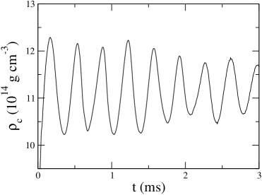
Figure 6: Time evolution of the central density for the collapse model R.

In Fig. 6 we show the time evolution of the central density for the model R. It is seen that the collapse continues until the central density rises up to $1.23\times 10^{15}\ {\rm g\ cm^{-3}}$, at which point the collapsing star bounces back and oscillations are excited subsequently.

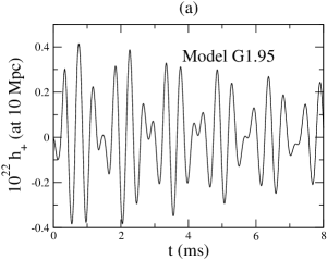
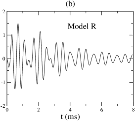
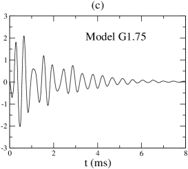
Figure 7: Gravitational waveforms $h_{+}$ on the $x$-axis for models G1.95 (a), R (b), and G1.75 (c). The source is assumed to locate at a distance 10 Mpc in all cases.

The coupling between the star’s rotation and oscillations leads to a rapidly changing quadrupole mass moment and hence a strong gravitational wave signal. In Figs. 7 (a)-(c), we show the time evolution of the gravitational waveforms $h_{+}$ on the $x$ axis for models G1.95, R, and G1.75. As listed in Table 1, the only difference among the three models in Figs. 7 (a)-(c) is the effective adiabatic index $\Gamma$ for the nuclear matter after phase transition. The figures show that the peak value of the gravitational wave amplitude increases as the value of $\Gamma$ decreases. This is expected, since a smaller value of $\Gamma$ corresponds to a larger reduction of the pressure. The collapsing star reaches a larger compactness before it bounces back, and hence the peak value of the gravitational wave amplitude is larger. We have also calculated the angle-averaged waveforms (see Sec. 2.4) for models G1.95, R, and G1.75. We found that the peak value of $<h_{+}^{2}>^{1/2}$ rises from $0.3\times 10^{-22}$ to $1.53\times 10^{-22}$ when $\Gamma$ decreases from 1.95 (model G1.95) to 1.75 (model G1.75).

Figs. 7 (a)-(c) show that the gravitational wave signals for the three models are qualitatively similar, except that for models R and G1.75 the wave amplitudes drop significantly within 8 ms. The damping of the gravitational wave amplitudes is mostly due to the development of differential rotations; and partly due to the formation of shock waves leading to the ejection of matter at the stellar surface.

We first consider the collapse model G1.75 and estimate the amount of energy available for stellar oscillations triggered by the collapse. We note that at any instant the total kinetic energy $T={1\over 2}\int\rho v^{2}d^{3}x$ of the star consists mainly of the rotational energy (uniform and differential rotation) $T_{\rm rot}$, with the rest associated with oscillations. We estimate the maximum amount of energy available for oscillations by the difference between $T$ and $T_{\rm rot}$ when the central density reaches the first maximum.

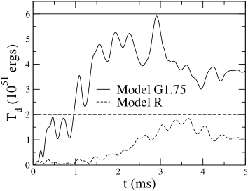
Figure 8: Time evolution of the kinetic energy associated with differential rotation $T_{\rm d}$. The horizontal lines correspond to the level of the maximum oscillation energy (see text) triggered by the collapse for models G1.75 (solid line) and R (dashed line).

For model G1.75, the central density reaches the first maximum at $t=0.149$ ms, and $T=7.3\times 10^{52}$ ergs at that instant. The rotational energy is mainly due to uniform rotation at that point (see Fig. 8) and is given by $T_{\rm rot}=J\bar{\Omega}/2=6.7\times 10^{52}$ ergs, where $J$ is the (conserved) total angular momentum and $\bar{\Omega}$ is the average angular velocity of the star at that time. The oscillation energy as defined is therefore approximately $T-T_{\rm rot}\approx 6\times 10^{51}$ ergs. Carrying out the same analysis, we find that the oscillation energy for the collapse model R is $\approx 2\times 10^{51}$ ergs.

To show that the energy associated with oscillations is mostly converted into the energy associated with differential rotation, we define the kinetic energy associated with differential rotation by

$$T_{\rm d}\equiv{1\over 2}\int\rho(v_{\phi}-\bar{v}_{\phi})^{2}d^{3}x,$$ (51)

where $\bar{v}_{\phi}=\bar{\Omega}(x^{2}+y^{2})^{1/2}$. For a uniformly rotating star, $T_{\rm d}$ vanishes identically. (Note that the sum of the energy associated with differential rotation as defined and the energy associated with uniform rotation does not equal to the total rotational energy.) In Fig. 8, we plot $T_{\rm d}$ versus time for models G1.75 and R. The horizontal lines correspond to the level of the maximum oscillation energy calculated above for models G1.75 (solid) and R (dashed). Fig. 8 shows that, for both models G1.75 and R, $T_{\rm d}$ grows rapidly to a level comparable to the oscillation energy by $t\approx 3$ ms. As can be seen from Figs. 7 (b)-(c), the amplitude $h_{+}$ has dropped significantly by $t\approx 3$ ms.

The above consideration suggests that the strong damping of the oscillations seen in models G1.75 and R can be attributed to the growth of differential rotation during the evolution. Most of the oscillation energy is converted to the kinetic energy associated with differential rotation. Differential rotation will be damped by viscosity (not modeled in our simulations).

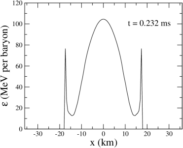
Figure 9: Profile of the specific internal energy $\epsilon$ (expressed as MeV per baryon) along the $x$-axis for model G1.75 at time $t=0.232$ ms.

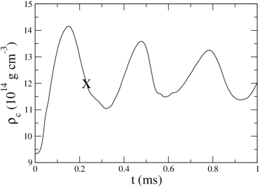
Figure 10: Time evolution of the central density of model G1.75. The point marked by an “X” represents the point when the shock shown in Fig. 9 is captured.

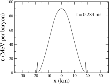
Figure 11: Profile of the specific internal energy $\epsilon$ along the $x$ axis for model G1.95 at time $t=0.284$ ms.

Furthermore, some of the oscillation energy is carried away by the shock waves formed at the star surface. Fig. 9 shows the profile of the specific internal energy $\epsilon$ (expressed as mega-electron volts per baryon) along the $x$ axis for model G1.75 at time $t=0.232$ ms. It is seen that a strong shock wave forms and reaches the surface of the star shortly before the end of the first oscillation. In Fig. 10 we plot the time evolution of the central density for model G1.75. The point marked by an “X” in the figure corresponds to the time of Fig. 9. Shock waves with weaker amplitudes are formed similarly in each oscillation. The oscillations are also damped by the shock waves carrying kinetic energy away from the star through the ejection of matter from the stellar surface. In the model G1.75, we find that the shock waves can dissipate $\approx 10\%$ of the oscillation energy by the end of the simulation. For comparison, Fig. 11 shows the first shock wave for model G1.95 at $t=0.284$ ms. The amplitude of the shock wave is much smaller. In this case, the oscillations are less damped by differential rotation and shocks, and the gravitational wave signals can last for longer period as shown in Fig. 7 (a).

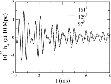
Figure 19: Convergence of the gravitational waveform $h_{+}$, at three different resolutions ($97^{3}$, $129^{3}$, and $161^{3}$), for the reference model R.

It should be noted that a small part of the oscillation energy is also lost in numerical damping arising from a finite differencing error, which depends on the grid resolution used in the simulation. As we see in Fig. 19, for the resolutions used in the simulations, numerical damping is important only for the late-time evolution, $t\gtrsim 4$ ms, at which point the oscillations have already been damped significantly by the development of differential rotation and shock waves. Another indicator of the accuracy of the simulations is that the total energy and angular momentum of the system are conserved to about 5% by the end of the simulations for all the collapse models considered in this paper.

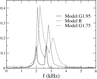
Figure 12: Fourier transforms of the wave amplitude $h_{+}$ for models G1.95, R, and G1.75 shown in Fig. 7.

Figs. 7 (a)-(c) show that the gravitational waveforms are not dominated by a single oscillation mode: the existence of interference between different oscillation modes in the gravitational wave signals is clear. We plot in Fig. 12 the Fourier transforms of the time evolution of $h_{+}$ shown in Figs. 7 (a)-(c). Fig. 12 shows that the gravitational wave signals are dominated by two oscillation modes. The frequencies of the oscillation modes increase as the value of $\Gamma$ decreases. The difference between the two oscillation frequencies $\Delta f$ also increases with a decreasing value of $\Gamma$. It changes from $\Delta f=0.66$ to 0.87 kHz, respectively, for models G1.95 and G1.75.

As we demonstrated in Sec. 4.1, for the models studied in this paper, the higher frequency mode is the fundamental quasi-radial mode of the final equilibrium star, while the lower frequency one corresponds to the fundamental quadrupole mode. In particular, the excitation of these two modes is a general feature of phase-transition-induced collapse of a rapidly rotating neutron star that does not depend sensitively on the EOS model.

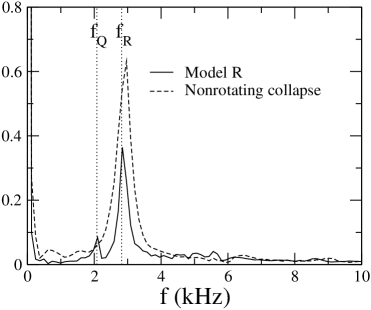
Figure 13: Fourier transforms of the time evolutions of the central density $\rho_{\rm c}$ for model R and its nonrotating counterpart. The positions of the two peaks in the Fourier spectrum of $h_{+}$ for model R are denoted by the vertical dotted lines $f_{\rm Q}$ and $f_{\rm R}$.

The quasi-radial mode becomes purely radial when the angular velocity of the star is zero, in which case it does not radiate gravitational wave. In Fig. 13 we plot the Fourier transforms of the time evolution of the central density $\rho_{\rm c}$ for model R and its corresponding nonrotating counterpart (defined by having the same set of EOS parameters and initial central density as model R). It is seen that for the nonrotating collapse model (dashed line) the spectrum is dominated by the fundamental radial mode at frequency 2.96 kHz. In the case of rotational collapse (solid line), the frequency of the radial mode decreases slightly to $f_{\rm R}=2.82$ kHz. The lower peak at $f_{\rm Q}=2.08$ kHz is the fundamental quadrupole mode. These two modes are the dominant fluid modes excited in the rotational collapse that radiate gravitational waves.

Fig. 12 also shows that the Fourier amplitudes of the higher frequency mode (the quasi-radial mode) for models R and G1.75 are smaller than that of the lower frequency one (the quadrupole mode). But for model G1.95 the contributions of the two modes to the gravitational wave signal are roughly the same. This is due to the severe damping of the quasi-radial oscillations by strong shock waves in models R and G1.75. In these cases, the quadrupole mode becomes the dominant gravitational-wave-radiating mode. On the other hand, the amplitudes of the shock waves formed in model G1.95 are much smaller, and the quasi-radial oscillations can radiate gravitational waves as strongly as the quadrupole mode.

To further quantity the damping effects, we use the following function to fit the gravitational wave amplitude $h_{+}$:

$$h_{+}(\bar{t})={A_{*}\over 2}\left[\exp\left({-{\bar{t}\over\tau_{\rm Q}}}\right)\cos(2\pi f_{\rm Q}\bar{t})+\exp\left({-{\bar{t}\over\tau_{\rm R}}}\right)\cos(2\pi f_{\rm R}\bar{t})\right],$$ (52)

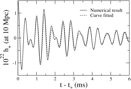
Figure 14: Gravitational waveform $h_{+}$ on the $x$-axis for model R. The solid line is the numerical result, while the dashed line is fitted to the function defined in Eq. (52).

where $A_{*}$ is the absolute maximum of the wave amplitude occurring at the time $t=t_{*}$, the time coordinate $\bar{t}$ is defined by $\bar{t}=t-t_{*}$, the $f$ values are the frequencies of the modes, the $\tau$’s are the damping time constants of the modes. For model R, from the numerical waveform and its Fourier transform, we have $t_{*}=0.704$ ms, $A_{*}=1.49\times 10^{-22}$, $f_{\rm Q}=2.08$ kHz, and $f_{\rm R}=2.82$ kHz. The two constants $\tau_{\rm Q}$ and $\tau_{\rm R}$ are determined by fitting Eq. (52) to the numerical data. Fig. 14 shows the best-fitted curve (dashed line) together with the numerical result (solid line). It is seen that the fitted curve agrees pretty well with the numerical result. The two damping time constants are determined to be $\tau_{\rm Q}=4.73$ ms and $\tau_{\rm R}=2.56$ ms. The smaller value of $\tau_{\rm R}$ compared to $\tau_{\rm Q}$ suggests that the quasi-radial mode is damped almost 2 times faster than the quadrupole mode. As we have mentioned above, this is due to the strong damping of the quasi-radial mode by the shock waves. For comparison, the damping time constants for model G1.75 are $\tau_{\rm Q}=2.53$ ms and $\tau_{\rm R}=0.42$ ms, while those for model G1.95 are $\tau_{\rm Q}=10.42$ ms and $\tau_{\rm R}=10.39$ ms. For the latter model, the two modes are less damped differential rotation and shock waves, and hence they have basically the same (relatively) large damping time constants. On the other hand, the modes are damped much faster in model G1.75. In particular, due to the generation of strong shock waves (see Fig. 9), the quasi-radial mode is damped 6 times faster than the quadrupole mode. We have also used Eq. (52) to determine the damping time constants for the other collapse models studied below. The values are presented in Table 2.

The change in the value of $\Gamma$ at the start of the dynamical evolution is to mimic the softening of the nuclear matter EOS in the mixed-phase model after the phase transition. Our results suggest that the gravitational wave amplitude emitted from the collapse and the duration of the wave signal depend quite sensitively on the value of $\Gamma$. The gravitational wave amplitude can reach a higher peak value if the subsequent EOS is significantly softer than that before the phase transition. However, the wave will be damped out quickly by the growth of differential rotation and the formation of strong shock waves. On the other hand, if the stiffness of the EOS is comparable to that before the phase transition, the gravitational wave signal will last for a significantly longer period. A long period could in turn facilitate the detection of the gravitational waves. We have also performed a simulation with $\Gamma=\Gamma_{0}=2$, which corresponds to the special case where the nuclear matter EOS does not change after the phase transition. We find that the emitted gravitational wave amplitude is too small to be resolved accurately by our grid resolutions. Nevertheless, we estimate that the upper bound of the angle-averaged wave amplitude $<h_{+}^{2}>^{1/2}$ is about $10^{-24}$ for a source located at 10 Mpc.

In our simulations, we study the effects of the EOS model on the gravitational wave signals by varying $\Gamma$, with the bag constant fixed to $B^{1/4}=170$ MeV. One might also want to vary the value of $B$ in order to study the effects of the EOS in details. However, by varying $\Gamma$ alone, we have already captured the general feature of what would happen to the gravitational wave signals if $B$ was varied instead. As suggested by Eq. (45), a smaller value of $B$ implies a stiffer quark-matter EOS, and hence the reduction of pressure after the phase transition is smaller. This in turn suggests that, if a smaller value of $B$ is used, the gravitational waveform of the reference model R (see Fig. 7 (b)) will become closer to that of model G1.95 (see Fig. 7 (a)): the emitted gravitational wave has a smaller amplitude and is less damped. On the other hand, if a larger value of $B$ is used, the gravitational wave signal will be closer to that of model G1.75 (see Fig. 7 (c)).

Besides the effect of $\Gamma$, we have also studied the gravitational wave signals emitted from the collapse process with different initial neutron star models. For all cases studied, we find that the gravitational waveforms are qualitatively the same as those shown in Figs. 7 (a)-(c). In particular, the excitation of the fundamental quasi-radial and quadrupole modes in the collapse process does not depend much on the mass and spin rate of the initial neutron star model.

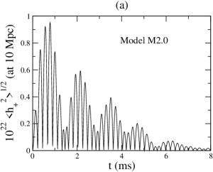
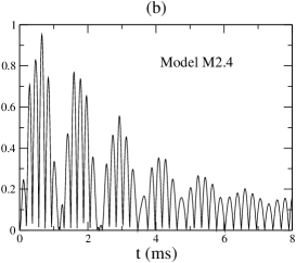
Figure 15: Effect of mass on the gravitational wave signals: Angle-averaged wave amplitude $<h_{+}^{2}>^{1/2}$ for models M2.0 (a) and M2.4 (b).

We first study the effect of mass. Figs. 15 (a) and (b) show the evolution of the angle-averaged wave amplitude $<h_{+}^{2}>^{1/2}$, respectively, for models M2.0 and M2.4. These models have the same initial rotation period $P=1.2$ ms as the reference model R. But note that model M2.0 has the largest $T/|W|$ value among all the collapse models (see Table 1). We find that the peak value of $<h_{+}^{2}>^{1/2}$ is about $0.95\times 10^{-22}$ for a source located at 10 Mpc away in both models. The Fourier spectra of the wave amplitude $h_{+}$ for these models also show that the fundamental quasi-radial ($f_{\rm R}$) and quadrupole ($f_{\rm Q}$) modes are the dominant contributions to the gravitational wave signals. The mode frequency $f_{\rm R}$ ($f_{\rm Q}$) increases from 2.54 (1.87) kHz to 3.02 (2.21) kHz, when the mass of the star increases from $2.0$ to $2.4M_{\odot}$. The damping time constants as determined by Eq. (52) for model M2.0 are $\tau_{\rm Q}=1.58$ ms and $\tau_{\rm R}=3.23$ ms, while those for model M2.4 are $\tau_{\rm Q}=4.30$ ms and $\tau_{\rm R}=2.26$ ms. Note that for model M2.0, $\tau_{\rm Q}$ is about 2 times smaller than $\tau_{\rm R}$ indicating that the quadrupole mode is damped faster. This is quite different from other collapse models in which $\tau_{\rm Q}$ is either comparable to or a few times larger than $\tau_{\rm R}$ (see Table 2).

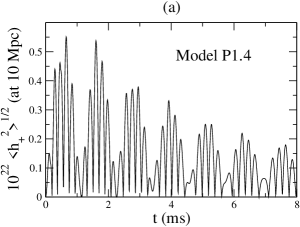
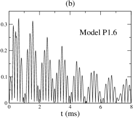
Figure 16: Effect of rotation on the gravitational wave signals. Angle-averaged wave amplitude $<h_{+}^{2}>^{1/2}$ for models P1.4 (a) and P1.6 (b). These two models have the same baryonic mass, $M=2.2M_{\odot}$, as the reference model R.

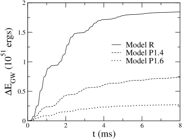
Figure 17: Total energy radiated in the form of gravitational waves for models R, P1.4, and P1.6.

To study the effect of rotation, we plot in Figs. 16 (a) and (b) the evolution of $<h_{+}^{2}>^{1/2}$, respectively, for models P1.4 and P1.6. These models have the same baryonic mass $M=2.2M_{\odot}$ as the reference model R. In contrast to the comparison between models M2.0 and M2.4, it is seen that the maximum amplitude of $<h_{+}^{2}>^{1/2}$ depends quite sensitively on the spin rate of the star. The strong dependence on the spin rate can also be seen from the energy radiated $\Delta E_{\rm GW}$ in the form of gravitational waves. Fig. 17 shows the total energy radiated for models R, P1.4, and P1.6. The total energy radiated for model R (with initial rotation period $P=1.2$ ms) is $1.85\times 10^{51}$ ergs. It drops down to $0.27\times 10^{51}$ ergs for model P1.6. This strong dependence on the spin rate can be understood from a dimensional analysis, which suggests that the gravitational wave luminosity $dE/dt$ is proportional to $\Omega^{6}$, where $\Omega$ is the angular velocity of the star. Form the Fourier transforms of the wave amplitudes $h_{+}$, we find that the frequencies of the two excited modes do not depend sensitively on the spin rate of the star (see Table 2).

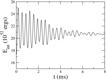
Figure 18: Time evolution of the total internal energy of model R.

It is also instructive to compare the energy carried away by the gravitational waves to the increase in internal energy of the collapsed object. In Fig. 18 we plot the time evolution of the total internal energy $E_{\rm int}=\int\rho\epsilon d^{3}x$ for the collapse model R. After the initial collapse phase, it is seen that $E_{\rm int}$ oscillates around its final equilibrium value, which we approximate by the time-average value of $E_{\rm int}$ in the period 2-6 ms. The change in the total internal energy in this case is $\Delta E_{\rm int}=3.57\times 10^{52}\ {\rm ergs}$. This value corresponds approximately to the difference in the internal energy between the final equilibrium configuration and the initial one. On the other hand, the energy that would be carried away by the gravitational wave $\Delta E_{\rm GW}=1.85\times 10^{51}\ {\rm ergs}$ amounts to only about 5% of $\Delta E_{\rm int}$. (Note that we do not have gravitational radiation reaction in the hydrodynamic equations [1]-[3], and hence the dynamical system is conservative.)

We have performed the same comparison for all the collapse models studied in this paper. We find that the energy ratio $\Delta E_{\rm GW}/\Delta E_{\rm int}$ ranges from 0.007 to 0.052. In the first few milliseconds covered by our simulations, the remaining kinetic energy is mostly in the form of the bulk motion (uniform and differential rotation). This kinetic energy will be converted to heat in the viscous timescale of the matter in a realistic collapse, longer than that covered by our simulations.

In Table 2 we summarize the results of the seven rotational collapse models studied in this paper. In the table, $f_{\rm Q}$ ($\tau_{\rm Q}$) and $f_{\rm R}$ ($\tau_{\rm R}$) are, respectively, the frequencies (damping time constants) of the fundamental quadrupole and quasi-radial modes obtained from the gravitational wave signals, $<h^{2}_{+}>_{\rm peak}^{1/2}$ is the peak value of the angle-averaged wave amplitude for a source at 10 Mpc, and $\Delta E_{\rm GW}/Mc^{2}$ is the ratio of the total energy emitted in the form of gravitational wave to the rest-mass energy of the star. To facilitate the comparison between our Newtonian results and future relativistic simulations, we also list in the table the angular frequency ($\omega$) of the modes by the dimensionless quantity $\omega M$ in units of $G=c=1$, where $M$ is the mass of the star.

To end this section, we demonstrate the accuracy of our numerical results by showing the convergence of the gravitational waveforms as we increase the grid-point resolution. In Fig. 19 we plot the evolution of $h_{+}$ on the $x$ axis for the reference model R with three different grid resolutions $97^{3}$, $129^{3}$, and $161^{3}$. Fig. 19 shows that the gravitational waveform converges very well as we increase the resolution. In particular, we see that the three different resolutions agree to high accuracy during the initial evolution. We conclude that the grid resolution $129^{3}$ used for all collapse models in this paper is in the convergence regime for the physics results reported in this paper.

5 Summary and Discussion

We have performed dynamical evolutions of phase-transition-induced collapse of rapidly rotating neutron stars using a three-dimensional Newtonian hydrodynamic code. We assume that once a seed of strange quark matter is formed inside the core of a neutron star, the star will convert to a quark star in a timescale much shorter than the dynamical timescale of the system. The resulting quark star is described by a mixed phase EOS model. Due to the reduction of the pressure, the star collapses promptly and stellar oscillations are excited. We have calculated the emitted gravitational wave signals by the quadrupole formula.

In our simulations, we use an ideal-fluid EOS $P=(\Gamma-1)\rho\epsilon$ to model the nuclear-matter phase. The MIT bag model with a bag constant $B^{1/4}=170$ MeV is used to describe the quark-matter phase. We consider $\Gamma$ as the only free parameter in our mixed-phase EOS model. We have found that the gravitational wave amplitudes depend quite sensitively on the value of $\Gamma$. The gravitational waves have higher amplitudes if the subsequent EOS of the matter is significantly softer than that before the phase transition. For our models, the peak value of the angle-averaged waveform $<h_{+}^{2}>_{\rm peak}^{1/2}$ can reach the order $10^{-22}$ for a source distance of 10 Mpc. However, the waves are damped very quickly by the growth of differential rotation and the formation of strong shock waves at the stellar surface. On the other hand, if the stiffness of the EOS does not change much after the phase transition (i.e., $\Gamma\lesssim\Gamma_{0}$), the fluid oscillations are less damped and the emitted gravitational wave signals will last for a longer period, albeit with smaller amplitudes. Furthermore, for all cases studied in this paper, we find that the energy carried away by the gravitational waves amounts to only a few percent or less of the increase in internal energy of the collapsed stars. This suggests that in a realistic collapse scenario, most of the gravitational potential energy released in the collapse will be converted into heat due to viscous damping and be carried away by radiation (neutrino and electromagnetic) in a much longer timescale.

Besides the effect of the EOS model, we have also studied the effects of mass and spin rate of the initial neutron star model on the gravitational wave signals. We find that for a fixed initial spin rate, the amplitude of the gravitational waves does not depend sensitively on the mass of the star. On the other hand, rotation of the star can enhance the amplitude of the gravitational waves significantly. The peak value of the angle-averaged waveform $<h_{+}^{2}>^{1/2}$ for a source at 10 Mpc can rise from $0.32\times 10^{-22}$ to $1.09\times 10^{-22}$ when the initial rotation period decreases from 1.6 ms (for model P1.6) to 1.2 ms (for model R).

We have found that the gravitational wave emission is dominated by two particular oscillation modes excited by the collapse. By studying a simplified collapse model and the oscillation modes of the corresponding final equilibrium star, it is found that the two excited fluid modes are the fundamental quasi-radial and quadrupole modes. The excitation of these two particular modes is quite general and does not depend sensitively on the EOS model. Hence, we expect that regardless of the EOS model of the quark star, which is not well understood at the moment, the gravitational wave signals emitted from the phase-transition induced collapse of rapidly rotating neutron stars are dominated by the fundamental quasi-radial and quadrupole modes of the final equilibrium stars. While it is generally expected that nonradial oscillation modes and various instabilities associated with them are the most promising sources of gravitational waves emitted from isolated neutron stars (Andersson, 2003), we have shown explicitly that the fundamental quasi-radial modes in rapidly rotating compact stars can also lead to significant emission of gravitational waves. For some of the collapse models studied in this paper, they can contribute to the gravitational wave signals as strongly as the fundamental quadrupole modes.

Our simulations are performed in full three-dimensions without any symmetry assumptions, and we do not see any excitation of non axisymmetric modes for the collapse models studied in this paper. The collapse scenarios that can lead to the development of nonaxisymmetric dynamics will be studied in a future paper.

Are the gravitational wave signals from phase-transition induced collapses detectable? Table 2 shows that the gravitational wave signals emitted from our collapse models have frequencies $\sim 2-3$ kHz and peak amplitudes $\sim 10^{-22}$ for a source distance of 10 Mpc. The relatively high frequency range puts the signals below the sensitivity of LIGO. However, for sources located within our Galaxy ($\sim 10$ kpc), the signals attain values well above the noise level of LIGO. With our conclusion that the waveforms are sensitive to the EOS, the detection of such gravitational wave signals would provide information regarding the EOS of newly born quark stars.

Finally, we conclude with several remarks. (1) Although our numerical simulations are performed in Newtonian gravity, we expect the same two dominant fluid modes to be excited in phase-transition induced collapse in full general relativity (GR). (2) For the models studied in this paper, we checked that at the maximum contraction point although the collapse (in Newtonian dynamics) is not strong enough to produce a black hole, gravity is so strong that general relativistic effects could be significant, and we will revisit this point with a full GR simulation in the next paper. (3) While the MIT bag model is only a simple phenomenological model for quark matter, we believe the main features found in this paper is generic to phase-transition induced collapse. (4) We have ignored the neutrino emission in our study. This is consistent with the maximum internal energy achieved in the collapse. The dynamics in the first few milliseconds is not strongly affected by neutrino emission, which, however, will be essential in the subsequent cooling (in the timescale of seconds or more; Shapiro & Teukolsky (1983)) of the collapsed object. (5) We have also ignored the effect of internal fluid dissipation in our simulations. The shear viscosity damping timescale of strange quark matter is comparable to that of normal nuclear matter and is on the order of $10^{8}$ s for a star model with mass $M=1.4M_{\odot}$, radius $R=10$ km, and temperature $T=10^{9}$ K. The bulk viscosity damping timescale for the same star model is on the order of seconds (assuming a rotation period of 1 ms and an $s$-quark mass $m_{s}=100$ MeV; Madsen (2000)). We thus conclude that viscosity damping is not important to the dynamics in the timescale $\sim 10$ ms studied in this paper.

Table 1: Phase-transition-induced collapse models

Model	$\rho_{\rm c}\ {\rm(10^{14}g\ cm^{-3})}$	$P\ {\rm(ms)}$	$T/|W|$	$M(M_{\odot})$	$R_{\rm e}\ {\rm(km)}$	$R_{\rm p}\ {\rm(km)}$	$\Gamma$
R	9.34	1.2	0.08	2.2	17.95	12.34	1.85
G1.95	9.34	1.2	0.08	2.2	17.95	12.34	1.95
G1.75	9.34	1.2	0.08	2.2	17.95	12.34	1.75
M2.0	7.73	1.2	0.11	2.0	21.31	11.78	1.85
M2.4	10.55	1.2	0.07	2.4	17.39	12.34	1.85
P1.4	10.30	1.4	0.05	2.2	16.26	12.90	1.85
P1.6	10.69	1.6	0.03	2.2	15.14	13.46	1.85

Table 2: Gravitational wave signals from the phase-transition induced collapse models

Model	$f_{\rm Q}$ ($\omega_{\rm Q}M$)	$\tau_{\rm Q}$	$f_{\rm R}$ ($\omega_{\rm R}M$)	$\tau_{\rm R}$	$<h_{+}^{2}>_{\rm peak}^{1/2}\ (10^{-22})$	$\Delta E_{\rm GW}/Mc^{2}$
R	2.08 (0.142)	4.73	2.82 (0.192)	2.56	1.09	$4.7\times 10^{-4}$
G1.95	2.00 (0.136)	10.42	2.66 (0.181)	10.39	0.30	$7.1\times 10^{-5}$
G1.75	2.25 (0.153)	2.53	3.12 (0.212)	0.42	1.53	$7.0\times 10^{-4}$
M2.0	1.87 (0.116)	1.58	2.54 (0.157)	3.23	0.95	$3.1\times 10^{-4}$
M2.4	2.21 (0.164)	4.30	3.02 (0.224)	2.26	0.95	$3.9\times 10^{-4}$
T1.4	2.18 (0.148)	3.88	3.01 (0.205)	3.31	0.55	$1.9\times 10^{-4}$
T1.6	2.12 (0.144)	4.08	3.11 (0.212)	4.56	0.32	$6.9\times 10^{-5}$

References

- Alcock & Olinto (1988) Alcock C., & Olinto A. 1988, Ann. Rev. Nucl. Part. Sci., 38, 161
- Andersson et al. (2002) Andersson N., Jones D.I., & Kokkotas K.D. 2002, MNRAS, 337, 1224
- Andersson (2003) Andersson N. 2003, Class. Quantum Grav., 20, R105
- Baiotti et al. (2005) Baiotti L., Hawke I., Rezzolla L., & Schnetter E. 2005, Phys. Rev. Lett., 94, 131101
- Blanchet et al. (1990) Blanchet L., Damour T., & Schäfer G. 1990, MNRAS, 242, 289
- Bodmer (1971) Bodmer A.R. 1971, Phys. Rev. D, 4, 1601
- Bombaci & Datta (2000) Bombaci I., & Datta B. 2000, ApJ, 530, L69
- Bombaci et al. (2004) Bombaci, I., Parenti, I. & Vidana, I. 2004, ApJ, 614, 314
- Bonazzola & Marck (1993) Bonazzola S., & Marck J.A. 1993, A&A, 267, 623
- Centrella & McMillan (1993) Centrella J.M., & McMillan S.L.W. 1993, ApJ, 416, 719
- Chau (1967) Chau W.Y. 1967, ApJ, 147, 667
- Cheng & Dai (1996) Cheng K.S., & Dai Z.G. 1996, Phys. Rev. Lett., 77, 1210
- Cheng & Dai (1998) Cheng K.S., & Dai Z.G. 1998, ApJ, 492, 281
- Collela & Woodward (1984) Collela P., & Woodward P.R. 1984, J. Comput. Phys., 54, 174
- DeGrand et al. (1975) DeGrand T., Jaffe R.L., Johnson K., & Kiskis J. 1975, Phys. Rev. D, 12, 2060
- Dimmelmeier et al. (2002) Dimmelmeier H., Font J.A., Müller E. 2002, A&A, 393, 523
- Dimmelmeier et al. (2005) Dimmelmeier H., Novak J., Font J.A., Ibáñez J.M., & Müller E. 2005, Phys. Rev. D, 71, 064023
- Drake et al. (2002) Drake J.J., et al. 2002, ApJ, 572, 996
- Finn & Evans (1990) Finn L.S., & Evans C.R. 1990, ApJ, 351, 588
- Flanagan & Hughes (2005) Flanagan E.E., & Hughes S.A. 2005, New J. Phys., 7, 204
- Font et al. (2001) Font J.A., Dimmelmeier H., Gupta A., & Stergioulas N. 2001, MNRAS, 325, 1463
- Fryer et al. (2002) Fryer C.L., Holz D.E., & Hughes S.A. 2002, ApJ, 565, 430
- Glendenning (2002) Glendenning N.K. 2002, Compact Stars: Nuclear Physics, Particle Physics, and General Relativity (New York: Springer-Verlag)
- Gondek-Rosinska et al. (2003) Gondek-Rosinska D., Gourgoulhon E., & Haensel P. 2003, A&A, 412, 777
- Gressman et al. (1999) Gressman P., Miller M., & Suen W.-M. 1999, Technical report, Washington University Gravity Group, St. Louis
- Gressman et al. (2002) Gressman P., Lin L.-M., Suen W.-M., Stergioulas N., & Friedman J.L. 2002, Phys. Rev. D, 66, 041303(R)
- Hachisu (1986) Hachisu I. 1986, ApJ, 61, 479
- Haensel (2003) Haensel, P. 2003, in Final Stages of Stellar Evolution, ed. C. Motch & J.M. Hameury (Les Ulis: EDP Sciences) p.249
- Hirsch (1992) Hirsch C. 1992, in Numerical Computation of Internal and External Flows, ed. R. Gallagher & O. Zienkiewicz (New York: Wiley-Interscience)
- Horvath & Benvenuto (1988) Horvath J.E., & Benvenuto O.G. 1988, Phys. Lett. B, 213, 516
- Limousin et al. (2005) Limousin F., Gondek-Rosinska D., & Gourgoulhon E. 2005, Phys. Rev. D, 71, 064012
- Lin & Suen (2004) Lin L.-M., & Suen W.-M. 2004, preprint (gr-qc/0409037)
- Lugones et al. (1994) Lugones G., Benvenuto O.G., & Vucetich H. 1994, Phys. Rev. D, 50, 6100
- Ma & Xie (1996) Ma F., & Xie B.R. 1996, ApJ, 462, L63
- Madsen (1999) Madsen J. 1999, Lect. Notes Phys., 516, 162
- Madsen (2000) Madsen J. 2000, Phys. Rev. Lett., 85, 10
- Marranghello et al. (2002) Marranghello G.F., Vasconcellos C.A.Z., & de Freitas Pacheco J.A. 2002, Phys. Rev. D, 66, 064027
- Mönchmeyer et al. (1991) Mönchmeyer R., Schäfer G., Müller E., & Kates R.E. 1991, A&A, 246, 417
- Oechslin et al. (2004) Oechslin R., Ury K., Poghosyan G., & Thielemann F.K. 2004, MNRAS, 349, 1469
- Olinto (1987) Olinto A.V. 1987, Phys. Lett. B, 192, 71
- Paczyński & Haensel (2005) Paczyński B., & Haensel P. 2005, MNRAS, 362, L4
- Rampp et al. (1998) Rampp M., Müller E., & Ruffert M. 1998, A&A, 323, 969
- Roe (1981) Roe P.L. 1981, J. Comput. Phys. 43, 357
- Satz (1982) Satz H. 1982, Phys. Lett. B 113, 245
- Shapiro & Teukolsky (1983) Shapiro S.L., & Teukolsky S.A. 1983, Black Holes, White Dwarfs and Neutron Stars (John Wiley & Sons: New York)
- Shibata & Sekiguchi (2004) Shibata M., & Sekiguchi Y. 2004, Phys. Rev. D, 69, 084024
- Shibata & Sekiguchi (2005) Shibata M., & Sekiguchi Y. 2005, Phys. Rev. D, 71, 024014
- Siebel et al. (2003) Siebel F., Font J.A., Müller, & Papadopoulos P. 2003, Phys. Rev. D, 67, 124018
- Stark & Piran (1985) Stark R.F., & Piran T. 1985, Phys. Rev. Lett., 55, 891
- Steffens et al. (1995) Steffens F.M., Holtmann H., & Thomas A.W. 1995, Phys. Lett. B, 358, 139
- Stergioulas et al. (2004) Stergioulas N., Apostolatos T.A., & Font J.A. 2004, MNRAS, 352, 1089
- Thoma et al. (2004) Thoma M.H., Trümper J., & Burwitz V. 2004, J. Phys. G, 30, S471
- Witten (1984) Witten E. 1984, Phys. Rev. D, 30, 272
- Yasutake et al. (2005) Yasutake N., Hashimoto M. & Eriguchi Y. 2005, Prog. Theor. Phys., 113, 953
- Zwerger & Müller (1997) Zwerger T., & Müller E. 1997, A&A, 320, 209