Disc orientations in pre-main-sequence multiple systems

Classical T Tauri stars are encircled by accretion discs most of the time unresolved by conventional imaging observation. However, numerical simulations show that unresolved aperture linear polarimetry can be used to extract information about the geometry of the immediate circumstellar medium that scatter the starlight. Monin, Ménard & Duchêne (1998) previously suggested that polarimetry can be used to trace the relative orientation of discs in young binary systems in order to shed light on the stellar and planet formation process. In this paper, we report on new VLT/FORS1 optical linear polarisation measurements of 23 southern binaries spanning a range of separation from $0.8^{\prime\prime}$ to $10^{\prime\prime}$. In each field, the polarisation of the central binary is extracted, as well as the polarisation of nearby stars in order to estimate the local interstellar polarisation. We find that, in general, the linear polarisation vectors of individual components in binary systems tend to be parallel to each other. The amplitude of their polarisations are also correlated. These findings are in agreement with our previous work and extend the trend to smaller separations. They are also similar to other studies, e.g., Donar et al. 1999; Jensen et al. 2000, 2004; Wolf et al. 2001. However, we also find a few systems showing large differences in polarisation level, possibly indicating different inclinations to the line-of-sight for their discs.

1 Introduction

Observational studies of low-mass stellar formation show that a large fraction of T Tauri stars (TTS) form in binary or multiple systems (e.g., Ghez, et al. 1993; Leinert et al., 1993; Simon et al. 1995; Ghez et al. 1997; Padgett et al. 1997). Theoretical studies have shown that fragmentation appears as the most likely binary formation mechanism to meet the observational constraints (e.g., Bate, 2000). Fragmentation mechanisms include fragmentation of a molecular cloud core (e.g., Pringle 1989) and growth of an instability in the outer parts of a massive circumstellar disc (e.g., Bonnell 1994). In the first case, neglecting long term tidal interactions, fragmentation could yield non-coplanar systems provided that the initial cloud is elongated and the rotation axis oriented arbitrarily with respect to the cloud axis (Bonnell et al. 1992). In the second case, the discs around both binary components will always be co-planar, thus the stellar spin axes aligned. The outcome of the fragmentation process depends on the initial conditions in the cloud and so do the final orientations of the rotation axes of the discs in binary systems. Most published theoretical fragmentation calculations have produced aligned discs, but with adequate initial conditions, misaligned systems are also a possible outcome (Bate et al. 2000).

Measuring this simple geometrical parameter of young binary systems, the relative orientation of the discs, is important to disentangle between various formation models. For example, it can provide very useful constraints on the initial distribution of angular momentum in the parent pre-stellar cores.

Unfortunately, circumstellar discs in multiple systems have been imaged in very few cases only around TTS (HK Tau: Stapelfeldt et al., 1998; HV Tau: Monin & Bouvier, 2000; LkH$\alpha$ 263: Chauvin et al., 2002). In each of these systems only one disc is visible and it is seen edge-on, a favorable orientation for detection. However, it is not secure to conclude on strong misalignment from these measurements only. Indeed, only a slight tilt of the other disc away from edge-on can abruptly reduce its detectability as the central star becomes visible directly. Nonetheless, and if both components have discs in these cases, it is possible to exclude a perfect alignment to within $\approx$ 15 degrees.

On the other hand, discs are often associated with jets. In some cases, multiple jets emerge from a common unresolved location (e.g., Davis et al. 1994). This may indicate the presence of multiple sources in the center, with different disc orientations. Apart from these few examples, i.e., in most other systems, the individual structure of the two components in a binary is unresolved and the determination of the relative orientation of the discs is a difficult challenge.

Previously, Monin et al. (1998) have proposed that individual aperture polarisation of the PMS binary components could be used to determine the relative orientation of CS discs projected in the plane of the sky, even when the individual discs are not resolved. They reviewed the literature for polarimetric measurements on wide binaries ($>8^{\prime\prime}$) and performed CCD imaging polarimetry on closer binaries. Their first results showed that discs appear to be preferentially aligned, with a few exceptions only. They also showed that the method is very sensitive to contamination by interstellar polarisation (ISP) that could mimic a common disc alignment. Other authors have obtained similar results in the near-IR (2.2 $\mu m$) for the Taurus region (Jensen et al. 2000; 2004), but their results could also be impaired by IS polarisation.

In this paper, we present new results obtained in the optical range with a dual beam imaging polarimeter with a large field-of-view that allows to estimate, simultaneously, the polarisation on the objects and on surrounding field stars, i.e., provide a simultaneous estimation of the ISP. We believe these new measurements are better suited to remove the contribution of the ISP and should provide a better view of the relative orientations of the individual components in binary systems. The method is recalled in section 2, and its limitations are briefly discussed. The observations performed with the VLT FORS1 polaro-imager (Appenzeller et al. 1998), and the data reduction process are presented in section 3. The results and a discussion are provided in section 4 section 5.

2 Determining disc orientation from linear polarimetry

2.1 The method

The method was presented in details by Monin et al. (1998): models of disc and bipolar reflection nebulae by Bastien and Ménard (1990) show that the position angle of the integrated linear polarisation of the scattered starlight is parallel to the equatorial plane of the disc, provided that its inclination is sufficiently large to mask the direct light from the star. The method is thus likely to give good results when circumstellar discs are simultaneously present around both stars in a binary, i.e. when both are Classical TTS (CTTS) and we have restricted our study to binaries where at least the primary is a known CTTS and/or an emission line star. This is justified because in most T Tauri pairs, when one of the components has an active disc, so has the other (see, e.g., Prato & Monin 2000, and references therein), with mixed pairs (CTTS+WTTS) being rare.

2.2 The contamination by interstellar polarisation

Interstellar polarisation is the main limitation to estimate the intrinsic polarisation of young objects because they are found in molecular clouds. As such, they are subject to superimposed polarisation from the cloud they are embedded into as well as from the interstellar medium to the observer. When two different polarisation directions are measured for the components of a binary system, it is fairly secure to say that they are intrinsically different. However, when they are similar, there is a chance that this identity is due to a common interstellar polarisation. Previous studies of disc alignment in binaries have tried to estimate the local ISM polarisation pattern from measurements found in the literature (Monin et al. 1998, Jensen et al. 2000; 2004). However, these estimations rely on few measurements made at different wavelengths, at different epochs, and sometimes quite far away from the binary under scrutiny.

In this paper, we have used a polaro-imager with a large field-of-view that can simultaneously measure the polarisation of the binary and of numerous nearby field stars. It is thus possible to estimate the local interstellar polarisation pattern around each source studied in this paper, under the assumption that the majority of these nearby probes are intrinsically unpolarised.

2.3 Measuring projected angles only

It should be noted that the method described in this paper can only determine the orientation of the disc projected on the plane of the sky, i.e, its position angle. The inclination angle of the source has no effect on the polarisation position angle, only on the polarisation amplitude. A full determination of the relative 3D orientations of discs in a binary system would require complementary observations of rotational periods and $V\sin i$, or direct images, which it outside the scope of this paper. However, Wolf et al. (2001) have shown that this problem can be addressed statistically. They showed that the probability distribution function of position angle differences will peak toward zero if discs have a tendency to be aligned. It remains possible however, for a given binary, to assess that its discs are not aligned when the PA difference is large.

3 Observation and data reduction

3.1 Source selection

The sources we studied are taken from the list of Reipurth & Zinnecker (1993, RZ93). The same source names are used. The angular separation of the binaries ranges from $0.8^{\prime\prime}$ to $10.6^{\prime\prime}$, corresponding to linear separations from 70 to 1900 AU, assuming the distance values given in RZ93, and Geoffray & Monin (2001) for Hen 3-600. The binaries were chosen in various southern star formation regions (SFR) with the condition that at least the primary is a known CTTS or emission line star. They are listed in Table 1, sorted by SFR of increasing right ascension, and, within a given SFR, by increasing separation. We keep this classification order throughout the rest of the paper.

Table 1: Source parameters, listed by SFR of increasing RA, and increasing angular separation within a given SFR.

Source	HBC	SFR	Sep (′′)	Sep (AU)
ESO H$\alpha\,29$		Gum	4.2	1900
Hen 3-600		TW Hya	1.5	70
Sz 30		Cha I	1.2	170
Sz 2	564	Cha I	2.2	310
Glass-I		Cha I	2.4	340
Sz 15		Cha I	10.6	1500
Sz 48		Cha II	1.31	260
Sz 62		Cha II	1.7	330
Sz 60		Cha II	3.4	670
HO Lup	612	Lup	1.5	220
Sz 116	625	Lup	1.6	240
SZ 81	604	Lup	1.9	285
SZ 65	597	Lup	6.4	960
WSB 20		Oph	0.8	130
WSB 18		Oph	1.1	170
WSB 26		Oph	1.2	130
WSB 19		Oph	1.5	24
WSB 35		Oph	2.3	360
WSB 4		Oph	2.8	450
WSB 42		Oph	5.1	820
WSB 28		Oph	5.1	1400
HBC 679	679	CrA	4.5	580
AS 353	292	L673	5.7	1700

The measure the interstellar polarisation near the targets of our study, we use background stars. We have estimated the number of foreground stars that can be expected in a FORS1 field-of-view (see § 3.2) toward each target is very small. We have used the galactic model from Bahcall & Soneira (1984) to compute how many stars should be present in the field in front of every source, given its galactic coordinates and distance. The result shows that in all cases but two, the foreground contamination is less than one star per field. Therefore, we use the stars present in each field to estimate the interstellar polarisation. The foreground-contaminated sources are ESO H$\alpha$ 29 (20 possible foreground objects) and AS 353 (7 objects).

Note that the polarisation of background stars is distance dependent (e.g., Serkowski et al., 1975). We suggest a method to test the reliability of our estimate in section 4.3. However, the regular pattern as well as the uniform degree of the polarisation observed around many of our sources suggest that the interstellar polarisation originates from a slab of dust (presumably that of the molecular cloud) rather than the diffuse interstellar medium (see section 4 and Figure 1 and 2).

3.2 Observations

Observations were made in the I-band during 5 nights on 2000 May 24-29. The weather conditions were good and the seeing was measured between 0.5 and $1.7^{\prime\prime}$ with a median value of $0.7^{\prime\prime}$ over the 5 nights. A good seeing is important because it sets the effective separation down to which binaries can be resolved. Integration times between 0.5 s and 2 min were used depending on the brightness of and the contrast needed in, each binary system.

The FORS1/IPOL instrument is equipped with a Wollaston prism that splits the incident beam in two different directions with orthogonal polarisation states, the so-called ordinary ($o$) and extraordinary ($e$) beams. A stepped half-wave plate retarder is placed at the entrance of the incident beam and can be rotated, in this case by multiples of 22.5^o so that 16 positions are needed for a complete rotation. The separation of the two $o$ and $e$ beams on the CCD is performed by the Wollaston prism and a 9-slit focal mask. Each slit is $\sim 20^{\prime\prime}$ wide. For each position of the rotating retarder plate, an image is recorded. The images are then combined to yield the Stokes parameters I, Q and U.

The total field-of-view of FORS1/IPOL is $6.8^{\prime}\times 6.8^{\prime}$ in the Standard Resolution (SR) mode with a focal scale of $0.2^{\prime\prime}$/pixel. To obtain the polarisation, the normalized flux difference between the ordinary and extraordinary images, either from aperture photometry on point sources or pixel by pixel on extended objects, was calculated and a Fourier series computed to derive the Stokes parameter Q and U In aperture photometry, with an aperture 3 FWHM in size and using all 16 rotations of the waveplate (yielding 8 independent estimations of $Q$ and $U$), the error on the polarisation is estimated at 0.1 % or better from photon noise only.

3.3 Data Reduction Pipeline

A dedicated data reduction pipeline was written using NOAO/IRAF. The images are first bias and bad pixel corrected, and then flat-fielded. In the next step the images go through a polarisation extraction routine. Two options are then available: the polarisation information can be estimated on a pixel per pixel basis, a useful possibility to map extended structures like reflection nebulosities, at the cost of a loss of accuracy on point sources when the image quality (FWHM) changes during acquisition of a full data set (i.e. between different positions of the half-wave plate). The other option uses aperture photometry to estimate precise polarisation measurements on point-like objects. In aperture photometry mode, any FWHM change can be accounted for if a large enough aperture is used, typically 3 FWHM. For a few of the tightest binaries of our sample, we modeled a point spread function from reference stars to extract the photometric signal of the two components by PSF subtraction.

The errors were estimated using 2 independent methods: first, from the photon noise on the $e-$ and $o-$beams separately, and then propagating the errors in the calculations of Q, U, P and $\Theta$; second, by measuring the standard deviation on the 4, 8 or 16 images from the half-wave plate rotation. Both estimations give consistent results except in a few pathological cases like, e.g., severe hit by a cosmic ray, sources too close to dead zones between orthogonal polarisation strips, etc.

The estimated error is less than $\sigma$(P)=0.1% (absolute value) when the binary components are well separated ($\geq$1.3 arcsec). However, in Table 2 and in subsequent computations, we conservatively use the worse value of the error estimated from the two methods. The resulting signal to noise ratio on the measured polarisation is usually high ($P/{\sigma}>10$) and we present our results without correction for low signal to noise bias (e.g., Wardle & Kronberg, 1974).

3.4 Instrumental polarisation at the center of the FORS1 field

Of crucial importance is the determination of the instrumental polarisation, $P_{\rm inst}$. We have carefully estimated it by measuring nearby (i.e., high proper motion) unpolarised targets. We have observed GJ 781.1 and GJ 2147, two high proper motion stars. Because the immediate solar neighborhood is remarkably devoid of dust, the interstellar polarisation of nearby stars can be considered null. The average of 4 measurements on both GJ objects gives $P_{\rm inst}=0.02\%\pm 0.03\%$. As a further check of very low instrumental polarisation at the center of the field, many binaries in our sample have low linear polarisation, known from previous publications. Our measurements with FORS1 are very close to previously published data. We therefore believe that FORS1/IPOL instrumental polarisation is very low on-axis, well below 0.1% at the center of the field, and we did not attempt to remove it from the measurements. We address the case of the spatial dependence of the instrumental polarisation in section 5.1.

4 Results

4.1 Polarisation data

For each field observed, the polarisation level, $P$, and the position angle, $\Theta$, is measured for every star for which S/N$\geq 1000$ ($\sigma_{P}=0.1\%$). Figures 1 and 2 show the polarisation maps obtained around the 23 binaries listed in Table 1. Across most of the fields, the polarisation presents a smooth pattern, both in $P$ and $\Theta$. However, in some of the fields the polarisation appears more chaotic, in amplitude and/or in position angle; this is the case for instance around WSB 19.

Figure 1: I band polarisation maps for the first 12 sources in our list.

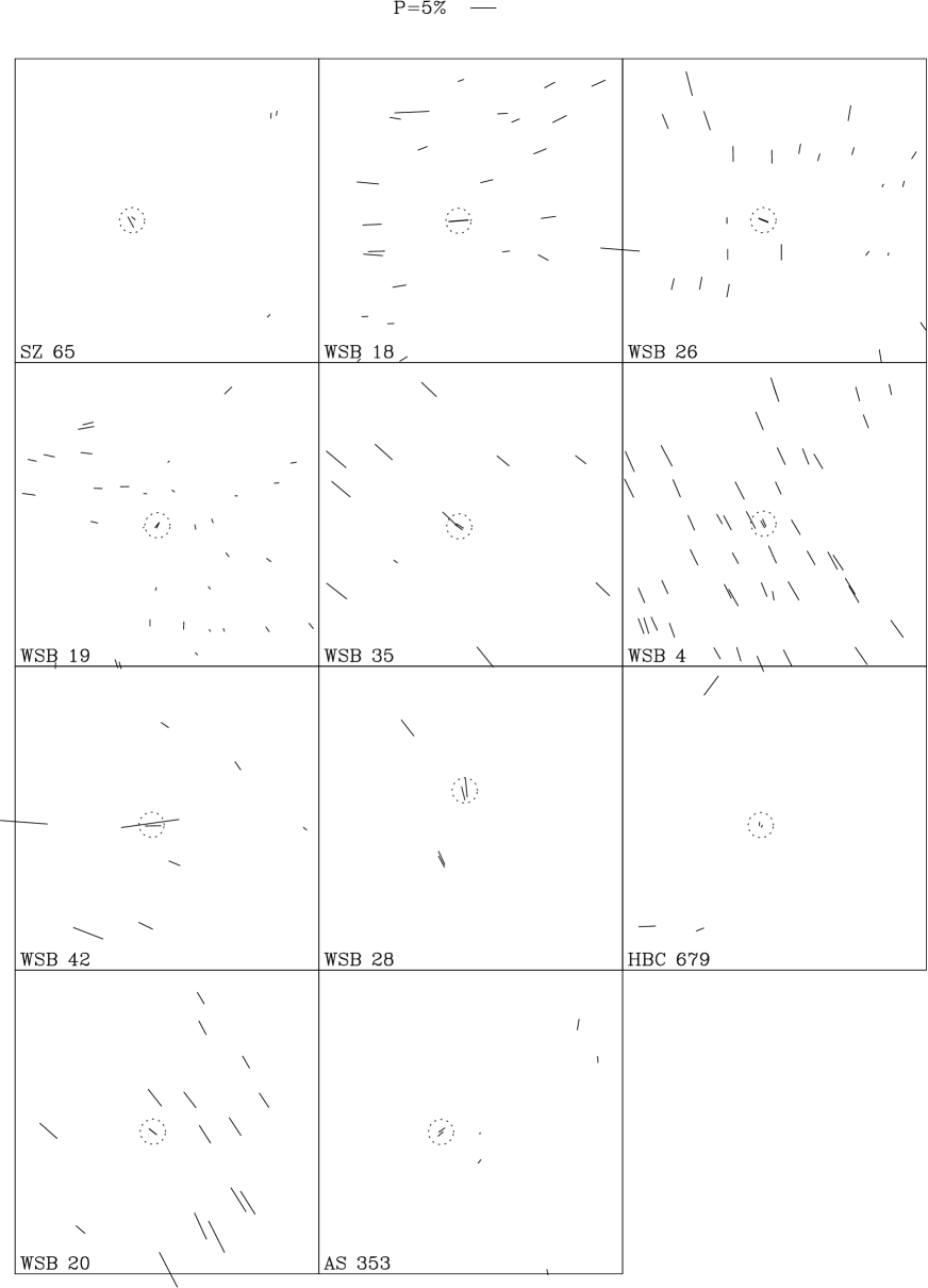
Figure 2: I band polarisation map of the last 11 sources in our list.

Table 2 lists the values computed for $P$ and $\Theta$ on the central binary components and on the surrounding interstellar medium for all sources. The method used to extract the interstellar polarisation (col. 6 & 7) is detailed in sect. 4.2.

Table 2: Polarisation measurements of the individual components (A,B) and estimation of the Interstellar polarisation (IS, computed in sect. 4.2, see text for details). In every column, the number in parenthesis gives the $1\,\sigma$ uncertainty. The three rightmost columns list the visual extinction from the literature and the references: (a) Prato et al. 2003; (b) Brandner & Zinnecker 1997; (c) Geoffray & Monin 2001.

Source	PA (%)	$\Theta_{A}(^{o})$	PB (%)	$\Theta_{B}(^{o})$	PIS (%)	$\Theta_{IS}(^{o})$	$A_{V}(A)$	$A_{V}(B)$	Ref.
ESO H$\alpha\,29$	1.39 (0.06)	65 (2)	2.47 (0.08)	122 (1)	3.2 (0.1)	105 (1)
Hen 3-600	0.27 (0.04)	9 (5)	0.02 (0.05)	171 (80)	0.84 (0.07)	53 (2)	0.7	0.7	c
Sz 30	1.3 (0.05)	156 (1)	1.4 (0.05)	155 (1)	5.3 (0.2)	154 (1)	0.58	0.19	b
Sz 2	1.53 (0.05)	112 (1)	4.10 (0.05)	116 (0.5)	5.4 (0.2)	112 (1)
Glass-I	4.15 (0.05)	135 (1)	4.88 (0.06)	24 (1)	7.46 (0.2)	118 (1)
Sz 15	1.28 (0.04)	32 (0.8)	4.81 (0.15)	24 (0.8)	4.0 (0.15)	22 (0.6)
Sz 48	3.62 (0.03)	116 (0.3)	3.70 (0.04)	116 (0.3)	1.29 (0.04)	120 (0.5)	3.41	3.58	b
Sz 62	2.76 (0.11)	122 (1)	2.72 (0.12)	121 (1)	2.88 (0.09)	121 (1)	1.08	1.58	b
Sz 60	3.47 (0.04)	135 (1)	2.94 (0.04)	125 (0.5)	3.0 (0.1)	117 (1)
HO Lup	1.21 (0.07)	12 (2)	1.51 (0.06)	19 (1)	0.8 (0.03)	7 (1)	1.25		c
Sz 116	0.04 (0.07)	158 (46)	0.18 (0.1)	71 (15)	3.55 (0.12)	165 (1)	0	0.9	a
SZ 81	0.4 (0.05)	39 (4)	1.11 (0.06)	30 (2)	0.79 (0.04)	7 (1)
SZ 65	0.89 (0.06)	53 (2)	2.3 (0.2)	29 (3)	0.84 (0.12)	168 (4)
WSB 20	2.84 (0.05)	113 (1)	2.85 (0.05)	113 (1)	4.10 (0.04)	124 (0.3)	2.3		c
WSB 18	3.8 (0.04)	95 (0.3)	3.79 (0.03)	95 (0.3)	2.08 (0.07)	99 (1)	4.04	3.41	b
WSB 26	1.95 (0.04)	68 (0.5)	1.95 (0.04)	68 (0.6)	1.72 (0.06)	175 (0.5)
WSB 19	1.09 (0.06)	139 (2)	1.26 (0.1)	152 (2)	0.42 (0.03)	55 (2)	1.7	2.7	b
WSB 35	1.58 (0.04)	59 (0.7)	1.81 (0.05)	54 (1)	4.34 (0.14)	48 (1)
WSB 4	1.52 (0.04)	31 (1)	1.57 (0.04)	25 (1)	2.75 (0.1)	21 (1)	0	0.4	a
WSB 42	3.10 (0.04)	91 (1)	11.4 (0.1)	98 (1)	5.2 (0.2)	81 (1)
WSB 28	2.67 (0.04)	14 (0.3)	3.75 (0.3)	5 (2)	2.52 (0.09)	28 (0.5)	5.1	2.5	a
HBC 679	0.47 (0.04)	156 (2)	0.73 (0.22)	176 (9)	1.71 (0.06)	106 (1)	4.8	1.6	a
AS 353	1.40 (0.04)	125 (1)	1.25 (0.09)	133 (2)	1.0 (0.1)	176 (3)		2.1	a

Figure 3: Measured polarisation level in the secondary versus in the primary. The dashed line traces an identical polarisation level in both components.

In Figure 3, we have plotted the polarisation level of the secondary component against that of the primary for all the binaries in our list except for WSB 20 which is too tight to obtain a reliable estimation of the individual polarisations. WSB 20 will not be considered in this study from now on. The plot shows that the polarisation levels of both components in a given binary are correlated. This result is expected if the discs of each components are similar in optical thickness and have the same inclination. It may also reflect a lack of intrinsic polarisation but a common contamination by the ISP. At first sight, Figure 3 also suggests that the polarisation level of the secondaries’ are often larger than the primaries’. This result is hard to explain if the measurements are dominated by the interstellar polarisation. It will be further analyzed and discussed in section 5.2.

4.2 Estimation of the nearby interstellar polarisation

In order to estimate the ISP at the center of each field, it is assumed that none of the surrounding stars are intrinsically polarised. In that case, the noise-weighted averages of their $Q$ and $U$ Stokes parameters, computed over the whole field-of-view and excluding the central binary, can be used as an estimation of the ISP.

$$\overline{Q} = {{\Sigma{{Q}\over{\sigma^{2}_{Q}}}}\over{\Sigma{{1}\over{\sigma^{2}_{Q}}}}}$$ (1)

$$\overline{U} = {{\Sigma{{U}\over{\sigma^{2}_{U}}}}\over{\Sigma{{1}\over{\sigma^{2}_{U}}}}}$$ (2)

However, estimation of the ISP based on the computation method described in Eq (1) and (2) requires caution. For example, accurately estimated single measurements can be spread over a large range of values (in $P$ and/or $\Theta$), possibly from superimposed interstellar clouds at various distances along the line of sight, and thus lead to a poorly representative estimation of the ISP at the distance of the binary. Therefore, further inspection of each polarisation map is also needed to disentangle ‘regular’ from ‘irregular’ ISP. Usually a quick visual inspection is sufficient. For example, WSB 19 shows two superimposed ISP components without any clear trend around the central position. WSB 19 is discarded from the sample for now on.

In general however, the observations show smaller fluctuations of the ISP across the field (e.g., ESO H$\alpha$ 29, and HO Lup), and the mean of the of the peak in the histogram of the position angles can be used to estimate the orientation of the ISP. In other cases, the ISP is very well defined across the field and its evaluation is straightforward. This is the case, e.g., for the fields around SZ 2 or SZ 62.

In practice, the average value of the ISP computed in equations (1) and (2) explicitly removes the influence of poor quality measurements (e.g., with large errors) while the median value eliminates spurious values (possibly measured with small errors). When both values, median and average, coincide the determination of the local ISP is considered reliable. Otherwise, no attempt is made to subtract an ISP component.

In Figure 4 and 5, we have plotted the weighted estimate of the ISP PA and percentage level vs the median value, showing that both estimates give the same result, except for 3 sources (SZ 48, WSB 42 and Hen 3-600).

As the weighted average is best evaluated from a signal-to-noise point of view, we keep it for further ISP subtraction. We do not attempt to subtract an interstellar component from the 3 discordant sources, 18 sources remain in the sample.

Figure 4: Median versus weighted Position Angle estimation of the interstellar polarisation for all sources in Table 1 except WSB 20.

Figure 5: Median versus weighted percentage level estimation of the interstellar polarisation for all sources in Table 1 except WSB 20.

4.3 Binary vs. interstellar polarisation

Before subtracting the local ISP, we consider in this section the results from the raw polarisation measurements. Figure 6 shows that there is no strong correlation between the interstellar polarisation and the polarisation levels of the individual components.

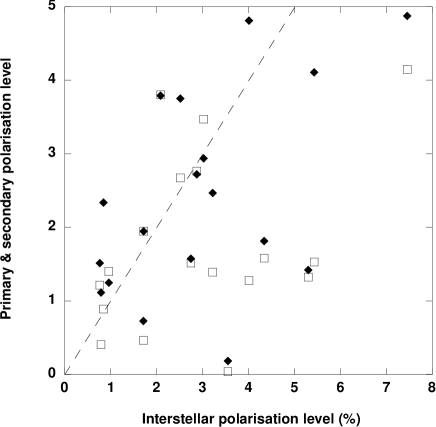
Figure 6: Polarisation level of the binary components (primary: open squares; secondary: full diamonds) vs interstellar polarisation for the 18 sources where the ISP is best evaluated. The dashed line traces the locus of fully influenced sources.

Similarly, Figure 7 shows the histograms of the position angle difference between the components and the interstellar polarisation for the primary and the secondary in the 18 sources with individual measurements and a reliable estimate of the ISP. Two thirds of the sources show both polarisations parallel to the ISP, to within 30 degrees (20 degrees for the primaries). Yet, one third of the sources are not aligned with the ISP. It indicates that at a fraction of their observed polarisation is intrinsic, different from the estimated ISP. On these sources, the results can be used to trace the actual orientation of the discs.

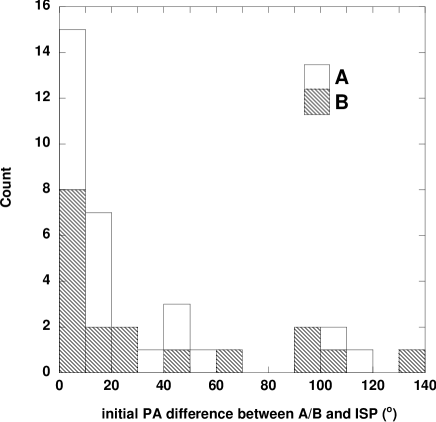
Figure 7: Distribution of the polarisation angle difference on 18 binary components vs interstellar polarisation. Primaries are open squares, secondaries are shaded.

At this point, it must be stressed that the absence of correlation between the interstellar and the individual polarisation levels (see Figure 6) could also result from an erroneous estimation of the interstellar polarisation. For instance, if the probe stars are placed at a larger distance than the binary, i.e., behind the cloud, then the interstellar polarisation level will likely be overestimated. This point will be addressed in details in sect. 5.3. However, even if the interstellar polarisation level is overestimated, its orientation is likely to remain correct. Hence the absence of a complete correlation between the various polarisation orientations (on the primary, the secondary and the ISP) indicates that at least about 30% of our measurements are most probably not strongly influenced by the ISP.

4.4 Polarisation measurements corrected for ISP

For the remaining 18 sources, we use the local ISP $\overline{Q}$ and $\overline{U}$ components and we compute the calibrated polarisation of the central binary components A/B:

$$Q^{\prime}_{A/B} = Q_{A/B}-\overline{Q}$$ (3)

$$U^{\prime}_{A/B} = U_{A/B}-\overline{U}$$ (4)

$$P^{\prime} = \sqrt{Q^{\prime 2}+U^{\prime 2}}$$ (5)

$$\Theta^{\prime} = 1/2\arctan(U^{\prime}/Q^{\prime})$$ (6)

Table 3 lists the values of the ISP-corrected level and PA for these sources.

Table 3: ISP-corrected polarisations for all the remaining 18 sources where both the object and surrounding interstellar polarisation can be correctly evaluated

Source	$P^{\prime}_{A}$ (%)	$\Theta^{\prime}_{A}(^{o})$	$P^{\prime}_{B}$ (%)	$\Theta^{\prime}_{B}(^{o})$
ESO H$\alpha\,29$	3.33 (0.12)	27 (1)	1.75 (0.14)	171 (2)
Sz 30	3.98 (0.14)	64 (1)	3.88 (0.14)	64 (1)
Sz2	3.90 (0.13)	22 (1)	1.48 (0.07)	11 (1)
Glass-I	4.67 (0.16)	12.7 (0.5)	12.3 (0.4)	26 (0.5)
Sz 15	2.84 (0.13)	107 (1)	0.88 (0.16)	35 (5)
Sz 62	0.12 (0.12)	23 (28)	0.17 (0.12)	43 (20)
Sz 60	2.07 (0.08)	165 (1)	0.82 (0.05)	169 (1.5)
HO Lup	0.48 (0.08)	20 (4)	0.89 (0.07)	30 (2)
Sz 116	3.5 (0.13)	75 (1)	3.73 (0.16)	75 (1)
SZ 81	0.7 (0.05)	82 (3)	0.80 (0.07)	53 (2)
SZ 65	1.56 (0.14)	65 (3)	2.37 (0.3)	39 (3)
WSB 18	1.77 (0.07)	90 (1)	1.76 (0.07)	89 (1)
WSB 26	3.52 (0.12)	76 (0.5)	3.5 (0.12)	76 (0.6)
WSB 35	2.9 (0.1)	132 (0.5)	2.6 (0.1)	134 (1)
WSB 4	1.38 (0.06)	102 (1)	1.2 (0.05)	108 (1)
WSB 28	1.28 (0.06)	159 (1)	2.7 (0.3)	164 (3)
HBC 679	1.84 (0.07)	9 (0.7)	2.3 (0.24)	10 (2)
AS 353	1.88 (0.12)	110 (2)	1.54 (0.14)	113 (2.5)

5 Discussion

5.1 Spatial dependence of the instrumental polarisation

Patat & Romaniello (2005) recently showed that FORS1 suffers from variable instrumental polarisation across the field of view, following a centrally symmetric pattern. A fit to the data shows the polarisation level to vary radially as $0.057\,r^{2}$ (in % with $r$ in arcmin), from 0% at the center up to $\approx 1$% at the corners. Such an instrumental pattern is of great concern in our measurements as we use the surrounding field stars to estimate the average value of the interstellar polarisation at the center of the field where the binary object is located.

The instrumental polarisation level remains below 0.1% within one arcmin from the geometrical center of the detector. In order to estimate the effect of a spatial variation of the instrumental polarisation in our data, we used three of our images where the polarisation appears smooth (i.e., SZ2, WSB 4, WSB 20, see figs. 1 and 2). Assuming that the actual interstellar polarisation is uniform across the field, we computed the average polarisation of the objects in a circle of radius 1 arcmin from the center (excluding the central binary), and we subtracted it from all the other measurements in the field in an attempt to remove the (large) interstellar polarisation and isolate an instrumental component.

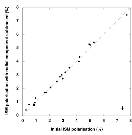
Figure 8: Comparison of the estimated interstellar polarisation with and without subtracting an instrumental radial component. The cross at the lower right indicates the typical error. The impact of intrumental polarisation on the measurements appears negligible.

Our results are consistent with an increase of instrumental polarisation with distance from the center, increasing as $0.06\,r^{2}$. We have then modeled a centrally symmetric instrumental polarisation component with such a variation and verified its influence on the parameters we extract from our images. None of them is significantly modified. As an example, Figure 8 shows that this effect on the estimation of the interstellar polarisation is very small and can be neglected. This is so because the interstellar polarisation in the clouds we observed is significantly larger than the instrumental polarisation and because this instrumental contamination is centrally symmetric, i.e., it cancels upon averaging when numerous, well distributed stars accross the fields are used. We are therefore confident that this instrumental effect does not modify significantly our conclusions on the alignment of discs in young binaries.

5.2 Why would the secondaries be more polarised?

Figure 3 shows that the measured polarisation level in the secondary component is almost always equal or larger than that of the primary, independently of the primary’s polarisation level.

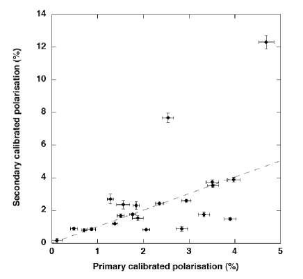
Figure 9: ISP-corrected polarisation level in the secondary versus in the primary.

To verify that trend, Figure 9 contains a plot of the ISP-corrected polarisation on the secondary versus the primary. The error bars are larger due to the subtraction of the ISP. After ISP subtraction the plot still suggests that a majority of systems have similar intrinsic polarisations. However, about a third of the systems show a significant difference between the polarisation level in both components, but contrary to Figure 3, there is no more tendency for one of the component (B) to be statistically more polarised than the other (A).

A possible explanation of this effect is a difference in the relative disc inclinations of the two components. In that case, a large polarisation difference may occur as the more extinct component (by the disc on the line-of-sight) will also be the more polarised (Monin et al. 1998).

This situation is similar to the case of HK Tau, where Duchêne et al. (2003) have found that each component of the binary has a disc, based on thermal emission at millimeter wavelengths, but they are not parallel to each other as seen on optical images: the fact that the (almost edge-on) secondary disc is visible when the primary one is not can be explained by a relative inclination $\Delta i$ larger than $15^{o}$. Such a difference is fully consistent with our results as about one third of our sources show (ISP-corrected) PA differences larger than $10^{o}$ (see fig. 10).

5.3 Can we confidently remove the ISP component?

In this section, we dicuss only the 18 binaries where both the central binary and the surrounding ISP can be measured reliably. However, even on very regular fields like around SZ 116 or SZ 2, the actual interstellar polarisation orientation might be correctly estimated, but its amplitude can be overestimated if the probe stars are situated far behind the cloud where the binary is placed.

If we call $Q,U$ the true interstellar polarisation Stokes parameters actually superimposed on the true $Q^{o}_{A,B},U^{o}_{A,B}$ binary polarisation parameters (A: primary, B: secondary), the estimators $\overline{Q},\overline{U}$ we compute from the background star distribution can overestimate $Q,U$ so that :

$$Q^{o}_{A,B}=Q_{A,B}-\alpha\,\overline{Q}$$

$$U^{o}_{A,B}=U_{A,B}-\alpha\,\overline{U}$$

Where $0<\alpha<1$ if we assume that the background stars can be anywhere but between the source and the observer.

Taking $\alpha=0$ is equivalent to ignore the influence of the local interstellar polarisation, hoping that it will not statistically change the result of the analysis. This is the choice made by previous authors who did not measure the IS polarisation. Using $\alpha=1$ is the choice made so far in this paper.

We now examine the intermediate case: $0<\alpha<1$. This is necessary whenever the ISP value is overestimated, e.g., by measuring stars much farther in the background.

To check the influence of an overestimation, one can look for a unique value of $\alpha$ allowing to build simultaneously $Q_{A},U_{A}$ and $Q_{B},U_{B}$ from $\overline{Q},\overline{U}$. The best estimation of $\alpha$ that would simultaneously null $Q_{X},U_{X}$ is:

$$\alpha(X)={Q_{X}\overline{Q}+{U_{X}\overline{U}}\over{{\overline{Q}}^{2}+{\overline{U}}^{2}}}$$

($X\equiv A,B$).

The goal is to find a value of $\alpha$ that would null both polarisations. In that case, the measured polarisation of the two components of the binary is very likely to be entirely of interstellar origin. Three binaries are found in the sample where the polarisation of both components can be simultaneously cancelled by the same fraction of interstellar polarisation. Those binaries are: Sz 30 ($\alpha(A)=0.25$ ; $\alpha(B)=0.27$); Sz 62 ($\alpha(A)=0.96;\alpha(B)=0.95$); Sz 116 ($\alpha(A)=0.02;\alpha(B)=0.05$). In the latter case, the initial polarisation of the binary is very weak and if it is not entirely from interstellar origin, it can hardly be used to study disc alignment anyway. In these 3 cases, we can not disentangle the polarisation of the sources from a possible interstellar origin. They are removed for any further statistical analysis. For the other systems, no common value of $\alpha$ can be found, suggesting differences in the intrinsic polarisation of each component.

For the discussion below we choose to keep $\alpha=1$ for the remaining 15 sources. In Figure 10, we have plotted the histogram of the ISP-corrected position angle difference between the primary and the secondary. 60% (9/15) of the sources show alignment better than 10^o, and 73% (11/15) better than 20^o. Only 4 sources show angle difference exceeding 25^o, and there is a unique case (Sz 15) where the polarisations are almost perpendicular to each other.

The error bars are of the order of a few degrees on the position angle ($\leq 5^{o}$). The good correlation between both polarisation position angles suggest that if the polarisation PA correctly traces the intrinsic disc orientation, then there is a strong alignment tendency between discs in binaries during the T Tauri phase of early stellar evolution.

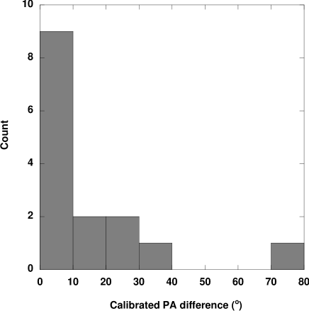
Figure 10: Histogram of the calibrated position angle difference in the 15 remaining binaries.

5.4 Alignment versus separation

In this section we compare the polarisation position angle difference with the projected linear binary separation. The result is presented in Figure 11 for the remaining 15 sources of the sample. No clear correlation appears but the distribution of angle differences is consistent with a larger difference for wider sources, although this could also reflect random alignment for non physical pairs. If the general trend is real, this is consistent with the results of Bate et al.(2000) that show that due to the shortness of the alignment time-scale, strongly misaligned discs are only likely to occur in binaries with separations larger than 100 AU. In our sample, we find that in 80% of the binaries with separation less than 700 AU, the discs are aligned to better than $15^{o}$. In this number, we have counted out Sz 2 because a strong polarisation level difference exists between the primary and the secondary, that can be interpreted in terms of inclination angle difference.

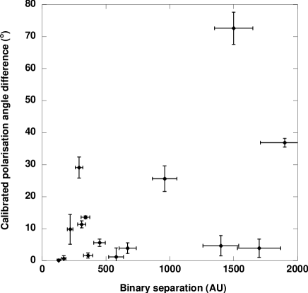
Figure 11: Discs orientation difference versus separation in AU. The error bars on the position angles are determined in our data reduction pipeline; we plot a 10% error on the distance determination.

5.5 Alignment pattern and timescale in various SFR

Our results are in line with previous estimates for wide binaries (Monin et al. 1998) and for binaries with similar separations in Taurus (Jensen et al. 2004). Thus, it appears that a disc alignment tendency is a common phenomenon in young SFR. Bate et al. (2000) suggest that in very dense star forming environments, misaligned discs could occur due to close dynamical interactions with other cluster members. The lack of misaligned discs in our results suggest that either the SFR’s we surveyed were not dense enough for strong misalignment to persist, or the disc alignment timescale is short enough that whatever the low age of the SFR, the discs always had time to re-align.

We also find that if closely aligned discs exist, there are also pairs that are misaligned, with PA differences larger than 30^o. This is also consistent with results from Bate et al. (2000), namely that the alignment timescale depends on the degree of initial misalignment: strongly misaligned discs take very little time to reduce their large difference in orientation but take a much longer time to reach perfect alignment, hence the existence of a tail in the distribution of position angle difference.

6 Conclusion

We have presented the results of a polarimetric survey on 23 southern pre-main sequence binaries closer than 2000 AU in separation, half of them being closer than 340 AU.

We have obtained $6.8^{\prime}\times 6.8^{\prime}$ polarimetric maps around all the binaries. The observations allow to estimate the linear polarisation of the central binary and an estimation of the local interstellar polarisation from surrounding background stars. We find that estimating the interstellar polarisation on the central binary is a difficult task. In particular, ‘by eye’ estimation of the local polarisation from the literature leads to significant errors.

In every binary, we have estimated an ISP-corrected polarisation for each component. We find that the polarisation levels for the primary and the secondary are correlated, although in some cases a strong difference exists between the two. Such a difference can be interpreted in term of a difference in the inclination of the discs relative to the line-of-sight. Indeed, the orientation we determine are projection on the plane of the sky, so for a given binary, we cannot rule out that discs have different inclinations, even if the position angle of the two components are similar. However, the fact that the calibrated polarisation levels remain highly correlated between primaries and secondaries is consistent with both discs sharing also similar orientations toward the line of sight. This is in agreement with Wolf et al. (2001) who calculated that a position angle difference distribution peaking toward zero is consistent with a disc alignment tendency.

We find that after interstellar polarisation subtraction, 73% (11/15) of the disc polarisation, hence the putative rotation axes of the components, are aligned within $20^{o}$, a result consistent with previous work (see Monin et al., 1998; Donar et al. 1999; Jensen et al. 2000; Wolf et al. 2001; Jensen et al. 2004). This proportion falls to 60% (9/15) when one takes into account the large polarisation level difference that exists between components with aligned discs in the plane of the sky. This result can be interpreted in terms of large difference between the inclination angles of the discs. In any case, this large proportion of aligned discs may reflect a primordial alignment during star formation.

- (1) Appenzeller, I., Fricke, K., Fürtig, W., et al. 1998, Msngr, 94, 1
- (2) Bahcall, J. N., & Soneira, R. M. 1984, ApJS 55, 67
- (3) Bastien, P., & Ménard, F. 1990, ApJ, 364, 232
- (4) Bate, M. R. 2000, MNRAS, 314, 33
- (5) Bate, M. R., Bonnell, I. A., Clarke, C. J., et al. 2000, MNRAS, 317, 773.
- (6) Bonnell, I., Arcoragi, J.-P., Martel, & H., Bastien, P. 1992, ApJ 400, 579
- (7) Bonnell, I. A. 1994, MNRAS, 269, 837
- (8) Brandner, W., & Zinnecker, H. 1997, A&A, 321, 220
- (9) Chauvin, G., Ménard, F., Fusco, T., et al. 2002, A&A, 394, 949
- (10) Davis, C. J., Mundt, & R., Eislöffel, J. 1994, ApJ 437, L57
- (11) Donar, A., Jensen, E. L. N., & Mathieu, R. D. 1999, AAS, 195, 7904
- (12) Duchêne, G. 1999, A&A, 341, 547
- (13) Duchêne, G., Monin, J.-L., Bouvier, J., & Ménard, F. 1999, A&A, 351, 954
- (14) Duchêne, G., Ménard, F., Stappelfeldt, K., & Duvert, G. 2003, A&A, 400, 559.
- (15) Geoffray, H., & Monin, J.-L. 2001, A&A 369, 239
- (16) Ghez, A. M., Neugebauer, & G., Matthews, K. 1993, AJ 106, 2005
- (17) Ghez, A. M., McCarthy, D. W., Patience, J. L., & Beck, T. L. 1997, ApJ 481, 378
- (18) Jensen, E. L. N., Donar, A. X., & Mathieu, R. D. 2000, IAUS 200, 85.
- (19) Jensen, E. L. N., Donar, A. X., & Mathieu, R. D. 2001,‘Aligned discs in Pre–Main Sequence Binaries’. In: The formation of Binary Stars, IAU Symposium, Vol 200, H. Zinnecker and R. D. Mathieu, eds., poster p 85
- (20) Jensen, E. L. N., Mathieu, R. D., Donar, A. X., & Dullighan, A. 2004, ApJ, 600, 789
- (21) Leinert, Ch, Zinnecker, H., Weitzel, et al. 1993, A&A, 278, 129.
- (22) Meyer, M.R., Calvet, N., & Hillenbrand, L.A. 1997, AJ, 114, 288
- (23) Ménard, F., & Duchêne, G. 2004, A&A, 425, 973
- (24) Monin, J.-L., & Bouvier, J. 2000, A&A 356, L75
- (25) Monin, J.-L., Ménard, F., & Duchêne, G. 1998 A&A, 339, 113
- (26) Padgett, D. L., Strom, S. E., & Ghez, A. 1997, ApJ 477, 705
- (27) Patat, F., & Romaniello, M. 2005, PASP, in press.
- (28) Prato, L., & Monin, J.-L. 2000, in The formation of Binary Stars, IAU Symposium, Vol 200, H. Zinnecker and R. D. Mathieu, eds., p 313
- (29) Prato, L., Greene, T. P., & Simon, M. 2003, ApJ, 584, 853.
- (30) Pringle, J. E. 1989, MNRAS, 239, 361
- (31) Reipurth, B., & Zinnecker, H. 1993, A&A, 278, 81
- (32) Serkowski, K., Mathewson, D. L., & Ford, V. L. 1975, ApJ, 196, 261.
- (33) Shu, F. H., Adams, F. C., & Lizano S. 1987, ARA&A, 25, 23
- (34) Simon, M., Ghez, A. M., Leinert, Ch., et al. 1995, ApJ 443, 625
- (35) Stapelfeldt, K.R., Krist, J.E., Ménard, F., et al. 1998, ApJ, 502, L65
- (36) Wardle, J.F.C., & Kronberg, P.P. 1974, ApJ 194, 249
- (37) Whitney, B.A., & Hartmann, L. 1992, ApJ 402, 605
- (38) Wichmann, R., Torres, G., Melo, C. H. F., et al. 2000, A&A, 359, 181
- (39) Wolf, S., Stecklum, B., & Henning, T. 2001, ‘Pre-main sequence binaries with aligned discs?’ In The formation of Binary Stars, IAU Symposium, Vol 200, H. Zinnecker and R. D. Mathieu, eds., p 295