Evolution and environment of early-type galaxies

Abstract

We study the photometric and spectral properties of 39320 early-type galaxies within the Sloan Digital Sky Survey (SDSS), as a function of both local environment and redshift. The distance to the nearest cluster of galaxies (scaled by the virial radius of the cluster) and the distance to the $10^{th}$ nearest luminous neighbor ($M_{r}<-21.5$) were used to define two extremes in environment. The properties of early-type galaxies are weakly but significantly different in these two extremes. In particular, the Fundamental Plane of early–type galaxies in the lowest density environment is systematically brighter in surface brightness (by $\sim 0.08$ mag/arcsec² in $r$) compared to the high density environment. A similar brightening is seen in the SDSS $g$ and $i$ photometric passbands. Although the Fundamental Plane is slightly thicker in the bluer passbands, we do not find any significant correlation between the thickness and the environment.

Chemical abundance indicators are studied using composite spectra, which we provide in tabular form. Tables of line strengths measured from these spectra, and parameters derived from these line strengths are also provided. From these we find that, at fixed luminosity, early-type galaxies in low density environments are slightly bluer, with stronger OII emission and stronger H$\delta$ and H$\gamma$ Balmer absorption lines, indicative of star–formation in the not very distant past. These galaxies also tend to have systematically weaker D4000 indices. The Lick indices and $\alpha$–element abundance indicators correlate weakly but significantly with environment. For example, at fixed velocity dispersion, Mg is weaker in early–type galaxies in low density environments by 30% of the rms scatter across the full sample, whereas most Fe indicators show no significant environmental dependence.

The galaxies in our sample span a redshift range which corresponds to lookback times of $\sim$1 Gyr. We see clear evidence for evolution of line-index strengths over this time. Since the low redshift population is almost certainly a passively aged version of the more distant population, age is likely the main driver for any observed evolution. We use the observed redshift evolution as a model independent clock to identify indicators which are more sensitive to age than to other effects such as metallicity. In principle, for a passively evolving population, comparison of the trends with redshift and environment constrain how strongly the luminosity-weighted ages and metallicities depend on environment. We develop a method for doing this which does not depend upon the details of stellar population synthesis models. Our analysis suggests that the galaxies which populate the densest regions in our sample are older by $\sim 1$ Gyrs than objects of the same luminosity in the least dense regions, and that metallicity differences are negligible.

We also use single burst stellar population synthesis models, which allow for non-solar $\alpha$-element abundance ratios, to interpret our data. The combination H$\beta$, Mg$b$ and $\langle$Fe$\rangle$ suggests that age, metallicity and $\alpha$-enhancement all increase with velocity dispersion. The objects at lower redshifts are older, but have the same metallicities and $\alpha$-enhancements as their counterparts of the same $\sigma$ at higher redshifts, as expected if the low redshift sample is a passively-aged version of the sample at higher redshifts. In addition, objects in dense environments are less than $1$ Gyr older and $\alpha$-enhanced by $\sim 0.02$ relative to their counterparts of the same velocity dispersion in less dense regions, but the metallicities show no dependence on environment. This suggests that, in dense regions, the stars in early-type galaxies formed at slightly earlier times, and on a slightly shorter timescale, than in less dense regions. Using H$\gamma_{\rm F}$ instead of H$\beta$ leads to slightly younger ages, but the same qualitative differences between environments. In particular, we find no evidence that objects in low density regions are more metal rich.

1 Introduction

There are two competing scenarios for the formation and evolution of giant early-type galaxies: Either they formed from an early monolithic collapse, and have evolved passively since, or they formed from the stochastic mergers of smaller systems. Both scenarios predict that the observed properties of galaxies should correlate with their environments.

In the first scenario, correlations with environment may arise because of a host of plausible physical effects associated with dense environments: these include ram pressure stripping of gas due to the hot, intra-cluster medium (Gunn & Gott 1972), galaxy harassment (Moore et al. 1999), tidal interactions (Bekki, Couch, & Shioya 2001) and strangulation (Balogh et al. 2001). In the second scenario also such effects may be important, but there is another natural reason to expect correlations with environment. In hierarchical clustering models, the oldest stars in the present day universe likely formed in the most massive systems present at high redshift (White & Rees 1978; White & Frenk 1991), those massive high-redshift systems merged with one another to form the most massive systems at the present time (Lacey & Cole 1993), and, at any given time, the most massive systems populate the densest regions (Mo & White 1996). Hence, the oldest stars, and the most massive galaxies, should populate the densest regions; since mass and age influence early-type galaxy observables, a correlation with environment is expected (Kauffmann 1996; Kauffmann & Charlot 1998). Since the two scenarios may make different predictions for trends with environment, it is interesting to quantify such trends. Our goal in what follows is not so much to distinguish between these models, as to develop techinques which allow one to quantify and interpret environmental trends, since both models predict that trends should exist.

Many early-type galaxy observables correlate with one another. Amongst the best-studied are the color-magnitude relation (e.g. Sandage & Viswnathan 1978a,b; Bower, Lucey & Ellis 1992a,b), the luminosity-velocity dispersion relation (Poveda 1961; Faber & Jackson 1977), the Fundamental Plane (Dressler et al. 1987; Djorgovski & Davis 1987), and correlations between chemical abundance indicators such as Mg and the velocity dispersion (e.g. Jørgensen 1997; Bernardi et al. 1998; Colless et al. 1999; Kuntschner et al. 2001). The search for correlations with environment has generally taken the form of measuring some of these correlations, and then trying to quantify if the relation is different in dense cluster-like regions than in less dense regions. For instance, the Mg-$\sigma$ relation shows only a weak dependence on environment (Bernardi et al. 1998), and recent work with the SDSS indicates that the color-magnitude relation also shows little dependence on environment (Bernardi et al. 2003d; Hogg et al. 2004; Balogh et al. 2004; Wake et al. 2005).

Interpreting these weak differences is more complicated. It is not clear if the small differences reflect genuinely small differences in the ages and metallicities of galaxies in low and high density environments, or if large changes in age are compensated-for by changes in metallicity (e.g. Worthey et al. 1994; Kuntschner et al. 2001), leaving the observables essentially unchanged. In addition, because early-types evolve relatively rapidly only when they are younger than a few Gyrs, small differences in formation times lead to only small differences in observables at later times.

In this study, we attempt to separate out the effects of age from other effects in two ways. In the first method, we study the spectroscopic and photometric properties of massive early-type galaxies over a wide range in environment and over a relatively small range in redshift. The small redshift range helps ensure that the galaxy population at the low redshift end of the sample is essentially a passively aged version of the population at higher redshifts. Comparison of the observed evolution with the observed dependence on environment provides a relatively model independent estimate of the typical age differences between environments. Our second method is more model dependent. We compare a variety of absorption line-strengths in the spectra of early-type galaxies with the latest generation of stellar population synthesis models. These models account for the fact that early-type galaxies are $\alpha$-enhanced relative to solar (e.g. Tripico & Bell 1995; Trager et al. 2000; Thomas, Maraston & Bender 2003 (TMB03); Thomas, Maraston, Korn 2004 (TMK04); Tantalo & Chiosi 2004).

The requirements of relatively small redshift coverage, but relatively large numbers of galaxies with well calibrated photometry and spectroscopy (so that small evolutionary and environmental trends can be detected) make the Sloan Digital Sky Survey (SDSS; York et al. 2000) the ideal database for this study. Section 2 describes various aspects of the dataset: how the early-type galaxy sample was selected (similar to Bernardi et al. 2003a), how composite spectra suitable for line-index measurements were assembled (similar to Bernardi et al. 2003d), and how estimates of the local environment for each galaxy were made. Section 3 presents evidence from the Fundamental Plane that cluster galaxies are slightly different from their counterparts in low density regions. Correlations between environment and various chemical abundance indicators are studied in Section 4. Section 5 compares the dependence on environment with that on redshift, and discusses how these observed trends can begin to distinguish age effects from those associated with changes in metallicity. It then provides a more quantitive argument which does not depend on the use of stellar population synthesis models. Such models are used to interpret our data in Section 6. A final section summarizes our findings, and discusses some implications. Appendices A and B discuss how we correct for selection effects and flux-calibration issues, respectively. Tables of the composite spectra we use, the line-strengths measured from them, and the ages, metallicities, and $\alpha$-element abundance ratios derived from the line-strengths are available, in their entirety, in the electronic version of the journal. Where necessary, we assume a background cosmological model which is flat, with matter accounting for thirty percent of the critical density, and a Hubble constant at the present time of $H_{0}=70$ km s^-1 Mpc^-1.

2 Sample selection

All the objects we analyze were selected from the Sloan Digital Sky Survey (SDSS) database. See York et al. (2000) for a technical summary of the SDSS project; Stoughton et al. (2002) for a description of the Early Data Release; Abazajian et al. (2003) et al. for a description of DR1, the First Data Release; Gunn et al. (1998) for details about the camera; Fukugita et al. (1996), Hogg et al. (2001) and Smith et al. (2002) for details of the photometric system and calibration; Lupton et al. (2001) for a discussion of the photometric data reduction pipeline; Pier et al. (2002) for the astrometric calibrations; Blanton et al. (2003) for details of the tiling algorithm; Strauss et al. (2002) and Eisenstein et al. (2001) for details of the target selection.

We selected all objects targeted as galaxies and having Petrosian (1976) apparent magnitude $14.5\leq r_{\rm Pet}\leq 17.75$. To extract a sample of early-type galaxies we then chose the subset with the spectroscopic parameter eclass < 0, which classifies the spectral type based on a Principal Component Analysis, and the photometric parameter fracDev_r > 0.8, which is a seeing-corrected indicator of morphology. fracDev_r is obtained by taking the best fit exponential and de Vaucouleurs fits to the surface brightness profile, finding the linear combination of the two that best-fits the image, and storing the fraction contributed by the de Vaucouleurs fit. We removed galaxies with problems in the spectra (using the zStatus and zWarning flags). From this subsample, we finally chose those objects for which the spectroscopic pipeline had measured velocity dispersions (meaning that the signal-to-noise ratio in pixels between the restframe wavelengths 4200Å and 5800Å is S/N $>10$). This gave a sample of 39320 objects, with photometric parameters output by version ${\tt V5.4}$ of the SDSS photometric pipeline and ${\tt V.23}$ reductions of the spectroscopic pipeline. For reasons given in Bernardi et al. (2003a), the luminosities and sizes we use in what follows are not derived from Petrosian quantities, but from fits of deVaucoleur profiles to the images.

2.1 Local environment

There is some debate in the recent literature over the optimal method for defining the local environment of galaxies (Eisenstein 2003; Kauffmann et al. 2003; Balogh et al. 2004). The options include using catalogs of clusters and groups of galaxies, adaptive measurements of local galaxy density, like distance to the $n^{th}$ nearest neighbor, and physical measurements of density based on expectation from simulations. Each of these methods has its own set of pros and cons. In this study, we attempt to minimize the problems associated with any one of these measurements of environment by using a combination.

We have chosen to represent the environment of a galaxy in two ways. One is to estimate the comoving distance to the nearest cluster, and the other defines a local density proportional to the inverse of the volume which encloses the nearest ten galaxies at $M_{r}<-21.5$ (Petrosian magnitudes). As our sample is magnitude limited, and the abundance of luminous galaxies drops exponentially at the bright end, the sample is much sparser at high redshifts. As a result, distances to the $n$th nearest neighbour will all be larger at high redshifts, unless we also specify that all $n$ neighbours were sufficiently luminous that they would have been seen at all redshifts in our catalog. Our brightness cut was chosen to satisfy the competing constraints of having enough objects from which to estimate distances, and of ensuring that those objects would satisfy the SDSS magnitude limits over as wide a range as possible. Since such objects cannot be seen beyond $z=0.15$, we limit our catalog to $z\leq 0.14$.

For each galaxy in our sample, we estimate comoving (three-dimensional) distances to all the objects which are more luminous than $1.75\times 10^{11}h_{100}^{-2}\,L_{\odot}$ in the C4 cluster catalog (Miller et al. 2004). This catalog is more than 90% complete out to $z=0.14$. Estimates of the mean redshift $z_{\rm cl}$, virial radius $r_{\rm cl}$, and velocity dispersion $\sigma_{\rm cl}$, are available for each C4 cluster. Given the redshift, the virial radius defines an angular scale, $\theta_{\rm cl}$. We label as cluster galaxies all those which lie within $\theta_{\rm cl}$ and $3\sigma_{\rm cl}$ of a C4 cluster.

The typical absolute magnitude of the early-type galaxies in our catalog is $M_{r}\simeq-21$. The absolute magnitude of the Sun is $4.62$ in this band, so the luminosity of a typical early-type is $\sim 1.77\times 10^{10}h_{70}^{-2}L_{\odot}$: the C4 clusters are $\sim 10$ times more luminous than a typical early-type galaxy. This means that smaller groups are not included in the C4 catalog; early-type galaxies in such groups will be assigned to denser environments only if such groups typically cluster around C4 clusters. Since such group members inhabit environments which are intermediate between rich clusters and low density environments, if we wish to define a sample in low density environments, we would like to include as few group galaxies as possible.

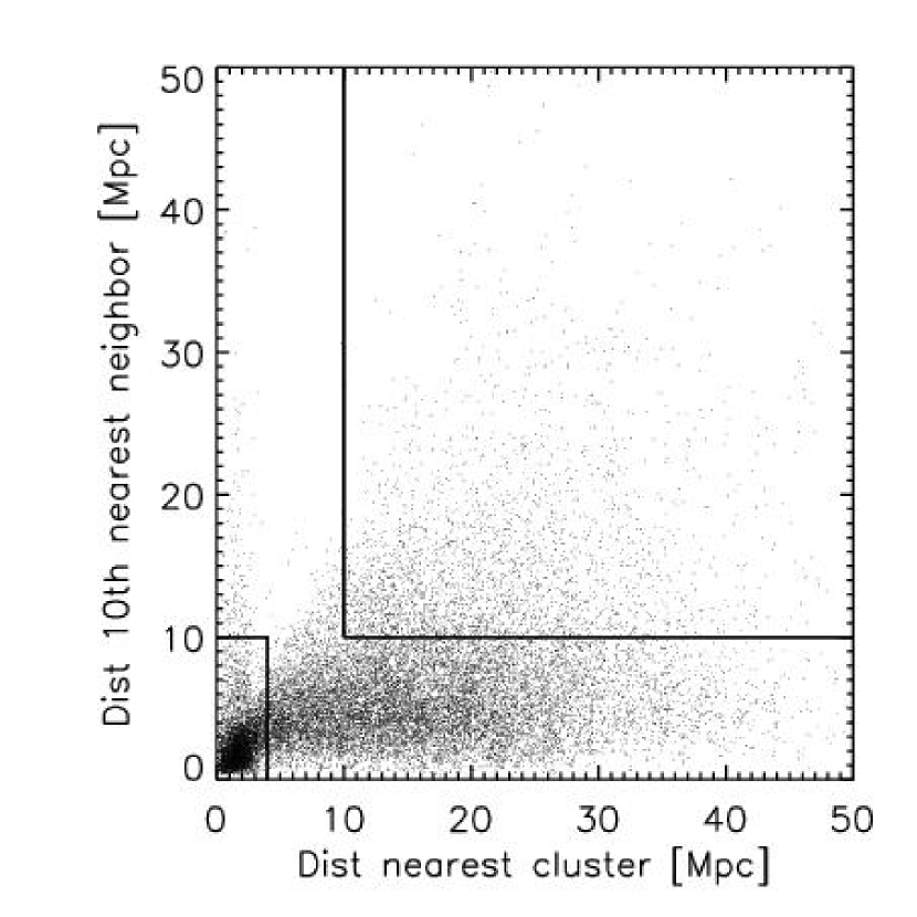
Figure 1: Classification into high density (lower left) and low density environments (upper right) is based on the comoving distance to the tenth nearest luminous ($L>3L_{*}$) neighbour, and on the comoving distance to the nearest massive cluster in the C4 catalog (Miller et al. 2004; each cluster is more luminous than $1.75\times 10^{11}h^{-2}L_{\odot}$ $\sim 10L_{*}$).

With this in mind, we define a sample of galaxies in less dense environments when the distance to the nearest cluster and the distance to the tenth nearest neighbour galaxy is larger than 10 Mpc. Our cut on tenth neighbour distance is supposed to eliminate most group galaxies from our low density environment sample. Thus, only objects in the densest (bottom left) and least dense (top right) environments of Figure 1 are used in the analysis which follows: in all there were 3112 and 5711 early-types in the two environments at $z\leq 0.14$.

There is a supercluster in the SDSS sample at $z\sim 0.08$. In what follows, we see some peculiarities in the redshift bin which contains this structure, so it may be that our estimates of environmental effects are altered by the supercluster.

2.2 Line indices

Later in this paper, we will study how various chemical abundance indicators of the early-type galaxy population depend on redshift and environment. The typical signal-to-noise ratio of an individual SDSS spectrum in our sample, $\sim$18, is considerably smaller than the value ($\sim$50) required to make reliable estimates of line-strengths. Therefore, for each environment, we construct high S/N composite spectra, suitable for line-index measurements, by co-adding the spectra of similar objects. We use narrow bins in luminosity, size, velocity dispersion, and redshift, chosen so that the resulting composite spectra had signal-to-noise ratios of $\sim$100. See Bernardi et al. (2003d) for details of the co-addition procedure. Briefly, spectra are normalized to have the same flux between 3900 and 7000Å, and then co-added, weighting by the observed error estimate in each pixel. Table 1 describes the bins we have chosen. The 925 composite spectra themselves are available from the electronic edition of the journal. Figure 2 shows the distribution of the number of objects per composite, as well as the distribution of S/N ratios. The results which follow have been obtained by using all the composites, although we have checked that the main conclusions do not change if only the subset with S/N$>40$ is used. The left panel of the Figure shows the difference between the full set of composites, and the higher signal-to-noise subset.

We measure the strengths of the original Lick indices (Worthey et al. 1994; Trager et al. 1998), as well as a number of other spectral features in each composite. This is because, with the exception of H$\beta$, none of the Lick indices are particularly sensitive to recent star-formation. Although we do not expect to find objects with large star-formation rates in our sample, some of the objects in it may have been forming stars at relatively small look-back times. Therefore, we also study some Balmer lines in absorption, H$\delta_{\rm A}$, H$\delta_{\rm F}$, H$\gamma_{\rm A}$ and H$\gamma_{\rm F}$, defined following Worthey & Ottaviani (1997), which are expected to indicate star-formation activity in the less distant past. Our estimates of the Balmer line strengths should be treated as lower limits because they may be filled-in by emission for which we have not corrected. However, we do correct H$\beta$ by adding 0.05 OII to the measured value. The standard correction uses OIII (e.g. Trager et al. 1998), but this is very noisy in our sample: OII shows a cleaner correlation.

In addition, many of these lines are close to the edge of the SDSS spectrograph, where flux calibration problems may bias our measurements. We discuss this more fully shortly.

Although our sample selection excludes strong emission lines, some weak emission is permitted. We find weak emission in OII which indicates very recent star formation, and/or AGN activity. We also study the strength of the break at 4000Å, and combinations of indices which are expected to be indicators of the metallicity and the relative abundances of $\alpha$-elements.

Where available (e.g. Jørgensen 1997), small aperture corrections have been applied to the measured values. These corrections are typically of the form $(8r/r_{e})^{\alpha}$ with $|\alpha|\sim 0.05$ (where $r_{e}$ is the half-light radius). Where no prescription was available in the literature, we used $|\alpha|=0.05$. This correction only matters for the trends with redshift which are presented in Section 5; but they are unimportant for the trends with environment, because we always study environmental effects at fixed redshift, and we see no significant dependence of galaxy size on environment. We have also corrected all line indices for the effects of velocity dispersion calibrated using the Bruzual & Charlot (2003) models and assuming Gaussian velocity distributions. In principle, the correction is different for non-Gaussian velocity distributions (e.g. Kuntschner 2004); we have chosen the Gaussian because our analysis is based on composite spectra, so choosing the appropriate non-Gaussian model to make the correction is not straightforward.

Tables 2–4 give our measurements of the index strengths in these composite spectra. In Section 6 we use stellar population synthesis models to interpret these measurements. These assume measurements at Lick rather than SDSS resolution, so, in that section only, we smooth the spectra to Lick resolution before correcting for the effects of velocity dispersion. The line-strengths at Lick resolution, for the indices used in that section, are given in Table 7.

3 The Fundamental Plane

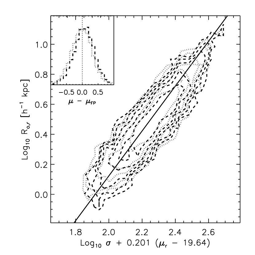
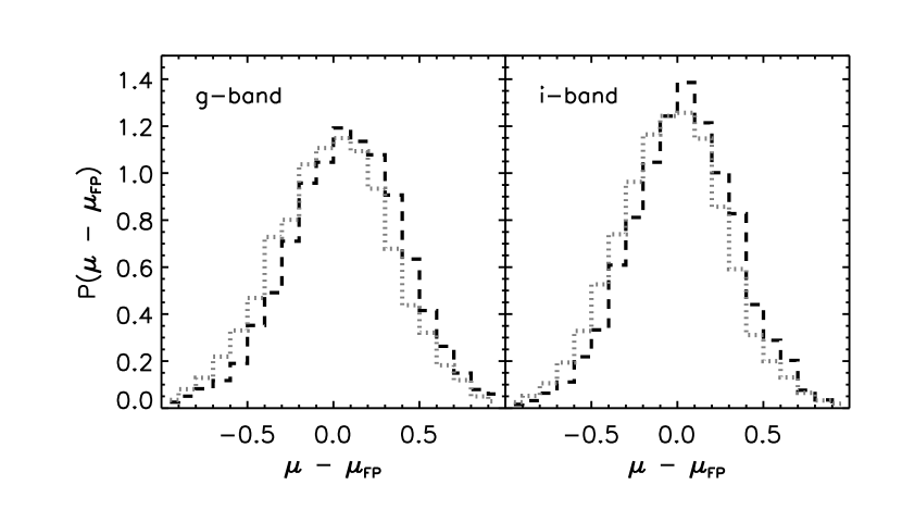
Figure 3: Top: The Fundamental Plane in the $r$ band. Solid line shows the fit from Bernardi et al. (2003c). Dashed and dotted lines represent the subset of galaxies which populate dense and less dense regions. Inset shows the distribution of residuals in surface brightness: galaxies in dense regions tend to be $\sim 0.08$ mag fainter than those in the least dense regions. Bottom panels show the distribution of residuals in surface brightness with respect to the FP in the $g$ and $i$ bands; the offset between low density and high density samples is similar to that in the $r$ band. Notice that the width of the distribution of residuals is approximately independent of environment.

There are a number of small but significant differences between our early-type galaxy samples in low and high-density environments. A traditional way to search for trends with environment is to study the distribution of galaxies in the space of log(size), log(velocity dispersion) and log(surface brightness). In this space, early-type galaxies populate a Fundamental Plane (e.g., Dressler et al. 1987; Djorgovski & Davis 1987). The solid line in the top panel of Figure 3 shows the best orthogonal-fit (determined following the methods described in Bernardi et al. 2003c) Fundamental Plane in the $r$ band using all early-type galaxies in our sample, whatever their environment. (Although, the old photometric reductions output by the SDSS pipeline photo were incorrect, using the new corrected photometry has not changed significantly the coefficients of the Fundamental Plane from those reported in Bernardi et al. 2003c). The dashed contours show the distribution of the subset of cluster galaxies in dense regions around the plane, while the dotted contours represent galaxies in less dense regions. The dependence on environment is weak. To show the dependence more clearly, the inset shows the distribution of residuals from the plane: evidently, galaxies in dense regions tend to have slightly ($0.075\pm 0.008$ mag) fainter surface brightnesses than their counterparts in less dense regions. The bottom panel shows a similar analysis of Fundamental Plane residuals in the $g$ and $i$ bands, for which the shifts are $0.081\pm 0.008$ mags and $0.069\pm 0.007$ mags, respectively. Note that the typical scatter around the plane is not significantly smaller in the cluster sample than in the low density sample. (Table 5 gives the mean offsets in each band for the two environments, as well as the rms residual.)

Our findings are consistent with a model in which the stars in any given early-type galaxy formed in a single burst, and, for the galaxies which are now in dense regions, this burst happened at higher redshifts. But a model in which the chemical abundances (e.g. metallicities) depend on environment would also work. In Section 6 we use single burst stellar population synthesis models to interpret these trends in terms of age and/or metallicity differences between the two populations. A more model independent analysis is the subject of Section 5.

4 Additional trends with environment

This section studies how various structural parameters and chemical abundance indicators depend on environment. In the figures that follow, we will often group together observables that are expected to trace similar physics. To facilitate comparison of different observables with one another, we standardize as follows: for each observable $Y$, we compute the mean $\langle Y\rangle$ and the rms simply by summing over the entire sample of composite spectra weighting each by the number of galaxies in the composite. We then show $(Y-\langle Y\rangle)/{\rm rms}(Y)$, rather than $Y$ itself. To simplify interpretation of selection effects, we show results from subsamples in different redshift bins. The values of $\langle Y\rangle$ and rms$(Y)$ are provided in Table 6.

The mean and rms values we quote are obtained by number weighting the composites when averaging, rather than averaging over the galaxies themselves. We have chosen to do this because line strengths computed from individual rather than composite spectra are very unreliable, so for most choices of $Y$ we must use composites. Therefore, although the mean values we quote should be accurate, the quoted rms values may underestimate the true scatter, because they do not include the contribution from the scatter among objects which make up each composite. However, because our composites are constructed from sufficiently small bins in the parameters which correlate most strongly with index strengths, it is likely that the scatter within a bin is negligible compared to the scatter between bins.

As a check, we performed all the analysis which follows using individual rather than composite spectra, subtracting the measurement errors in quadrature when computing rms values. This showed that our quoted rms values actually do not underestimate the true scatter substantially. Using the individual spectra rather than the composites has no effect on any of our qualitative conclusions, but because quantitative measurements based on composites are more robust, we have chosen to present all results using the composites only.

Note that a variety of emission and absorption lines, as well as the Lick indices, are known to correlate with luminosity and/or velocity dispersion. We have measured a number of such correlations (for a selection, see Bernardi et al. 2003d as well as Appendix B): for most, the primary correlation is with velocity dispersion, the correlation with luminosity (if present) being primarily a consequence of the index-$\sigma$ and luminosity-$\sigma$ correlations. In this respect, many line-strengths behave similarly to color (Bernardi et al. 2003d, 2005). Therefore, if we find that these line-strengths vary with environment, it is important to check if the environmental trend is entirely a consequence of a correlation between luminosity and/or velocity dispersion and environment, or if the environment did indeed play an additional role.

4.1 Structural parameters

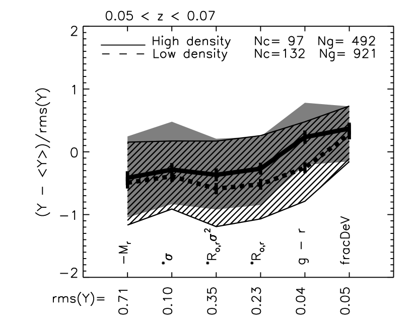
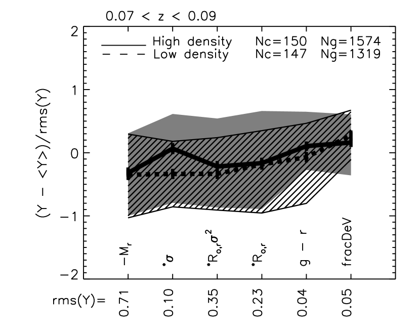
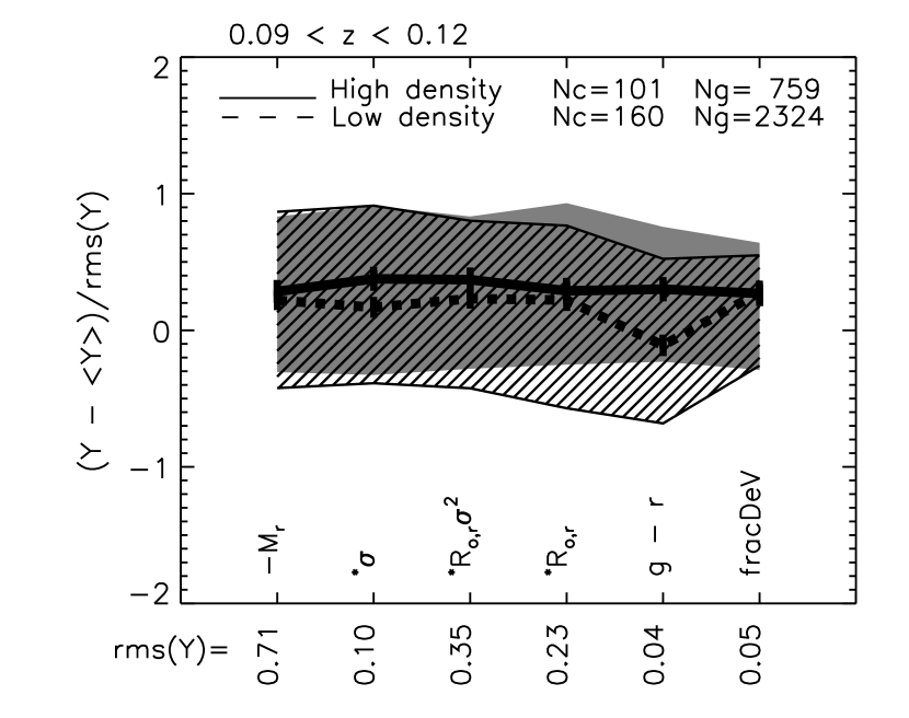
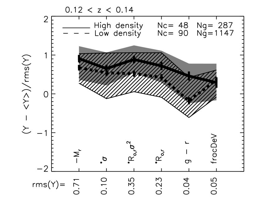
Figure 4: Median values of luminosity, velocity dispersion, mass, size, color, and light-profile shape fracDev (i.e. morphological type) in dense and underdense regions. To facilitate comparison with one another, all observables have been rescaled by subtracting the mean and then dividing by the rms spread across the entire sample (i.e. across all redshifts and luminosities). The x-axis lists the observable and the value of the rms. An asterisk denotes that the quoted rms is for $\log_{10}$ of the parameter. Shaded regions show the 25th and 75th percentile values. Different panels show subsamples at $0.05<z<0.07$, $0.07\leq z<0.09$, $0.09\leq z<0.12$ and $0.12\leq z<0.14$. Text in top right of each panel indicates the total number of composites in each redshift bin, and the total number of galaxies which made-up those composites. Top right panel contains a supercluster, so environmental effects may not be accurate.

Since we will be interested in whether or not environment plays a role over and above determining the structural parameters of galaxies, Figure 4 shows the typical values of luminosity, velocity dispersion, mass, size, color and light-profile shape fracDev in dense and less dense regions. All observables have been rescaled by subtracting the mean in the entire sample, and then dividing by the rms. The x-axis lists the observable and the value of the rms. Solid and dashed lines show the median values in dense and less dense regions, respectively. Error bars show the error on this median value, and shaded regions show the 25th and 75th percentile values. (An asterisk signifies that the quoted rms is for $\log_{10}$ of the index.) To simplify interpretation of selection effects, we show results from subsamples at $0.05<z<0.07$, $0.07\leq z<0.09$, $0.09\leq z<0.12$ and $0.12\leq z<0.14$. The text in the top right of each panel indicates the total number of composites in each redshift bin, and the total number of galaxies which made-up those composites.

Note that the supercluster at $z\sim 0.08$ is obvious: the ratio of the number of galaxies in high density regions to that in regions of lower density is considerably higher in the $0.07<z<0.09$ bin. In what follows, we see some peculiarities in this redshift bin.

The main point of this figure is not to compare the different panels with one another, but to compare the two environments in each panel with one another. This is because the primary difference between the different panels is caused by the magnitude limit: the higher redshift samples contain objects which are more luminous, have higher velocity dispersions, larger masses and sizes. However, the figure shows that, in any given redshift bin, trends with environment are weak: in all cases where there is a small difference, the objects in the low density environments tend to be slightly less luminous, to have smaller velocity dispersions, masses and sizes, and to be slightly bluer, although these differences are usually less than twenty percent of the rms variation across the entire sample (i.e., two tickmarks), except in the highest redshift bin.

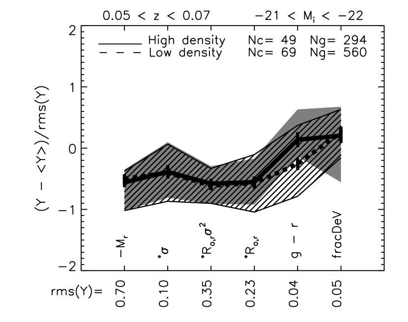
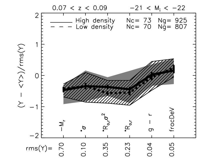
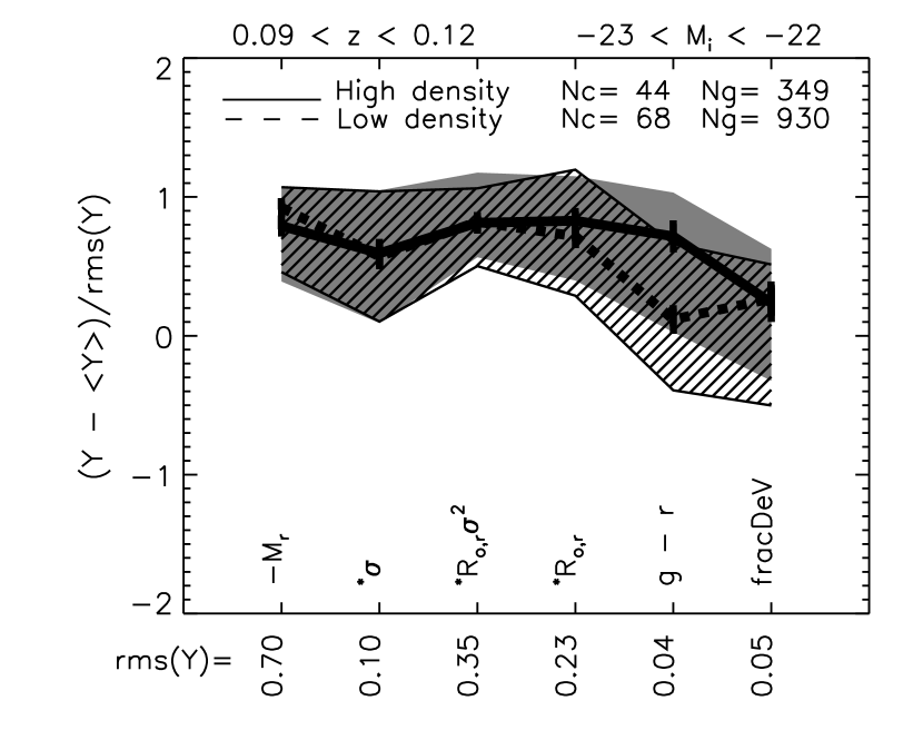
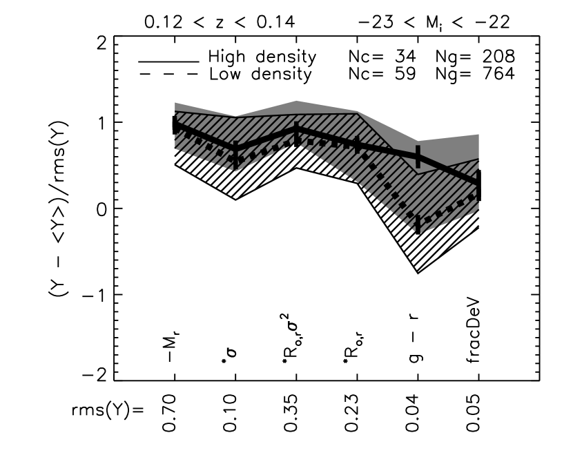
Figure 5: As for the previous figure, but now only results from objects with a narrow range of luminosities (indicated in the top right of each panel) are shown. The magnitude limit of the sample means that the low redshift bins contain objects with smaller luminosities than the higher redshift bins. (An asterisk signifies that the quoted rms is for $\log_{10}$ of the index.) In these narrow bins of redshift and luminosity, the mean velocity dispersions are similar in dense and less dense environments (this is not quite true for the bottom right panel, in which $\sigma$ seems to scatter to smaller values in lower density regions). The top-right panel is different from the others; it happens to contain a supercluster, and this may have compromised our estimates of environmental effects.

To remove the effects of correlations with luminosity or velocity dispersion, we have further divided each redshift bin into narrow bins in luminosity. Figure 5 shows that the small environmental trends evident in Figures 4 are seen consistently in all the panels. The top two panels of Figure 5 show the values of the structural parameters of galaxies which are slightly more luminous than $L_{*}$: in the lowest redshift bin (i.e., the panel on the left), the luminosities, velocity dispersions, masses, sizes and profile shapes (fracDev) of the high and low density environment samples are virtually identical, whereas a small but significant difference is detected in the color. Except for the color, the panel on the right shows similar trends, but recall that this redshift bin contains a supercluster, and this may bias our results.

The bottom two panels show results in the two higher redshift bins, for which the bin in luminosity is necessarily brighter. In these panels, the sample in low dense regions is significantly bluer, even though the median luminosity and velocity dispersion are the same as that in the higher density sample (this is not quite true for the bottom right panel, in which $\sigma$ seems to scatter to smaller values in lower density regions). This illustrates clearly that the environment plays a role in determining galaxy colors. A K-S test confirms what is obvious to the eye: the only cases in which the distributions of the parameters in low and high-density regions are significantly different ($p_{\rm KS}<0.05$) are for the $g-r$ color in the top left, and bottom two panels.

The trends in Figure 5 are reported in Table 6. Comparison of the two values of fracDev in each panel of this and the preceding figure (also see Table 6) show that the mean fracDev is the same in both dense and less dense regions. (We do not expect fracDev to distinguish between S0s and ellipticals—for our purposes, S0s and ellipticals are both early-type galaxies.) Since fracDev is an indicator of morphology, this shows that any trends with environment are probably not driven by a correlation between morphology and density (e.g. Dressler 1980). If some of the trends we see are indeed associated with the morphology-density relation, then the differences we detect in the properties of galaxies in high and low density regions are overestimates of the true differences. This places even tighter limits on the possible role played by the environment.

4.2 OII, Balmer lines, D4000, and $\alpha$-elements

This subsection studies the correlation between emission line strengths (OII), absorption lines which are not part of the original Lick system (Worthey et al. 1994; Trager et al. 1998), i.e. the Balmer line indices H$\delta$ and H$\gamma$ (Worthey & Ottaviani 1997), the strength, D4000, of the break in the spectrum at 4000Å (e.g. Balogh et al. 1999), and some combinations of the Mg and Fe lines, i.e. [MgFe]^′ (e.g. TMB03) and Mg/$\langle$Fe$\rangle$, with the environment. The OII emission line is an indicator either of very recent star-formation or of AGN activity, the Balmer (absorption) line indices are sensitive to star formation, the 4000Å break is an indicator of age (although all these observables also depend on metallicity and $\alpha$-element abundance ratios of the stellar population), Mg/$\langle$Fe$\rangle$ is an indicator of the $\alpha$-element abundance ratios (in early-type galaxies, this ratio is enhanced relative to the solar value), and [MgFe]^′ is an index which is an indicator of metallicity that is not expected to be very sensitive to the $\alpha$-element abundance ratios.

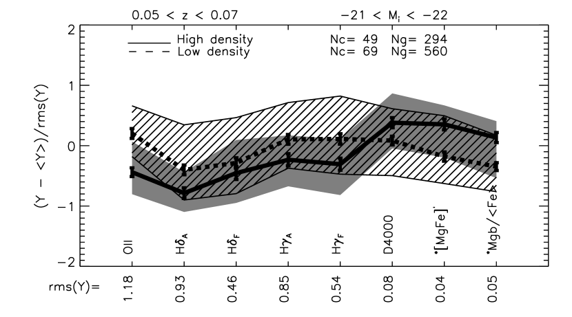
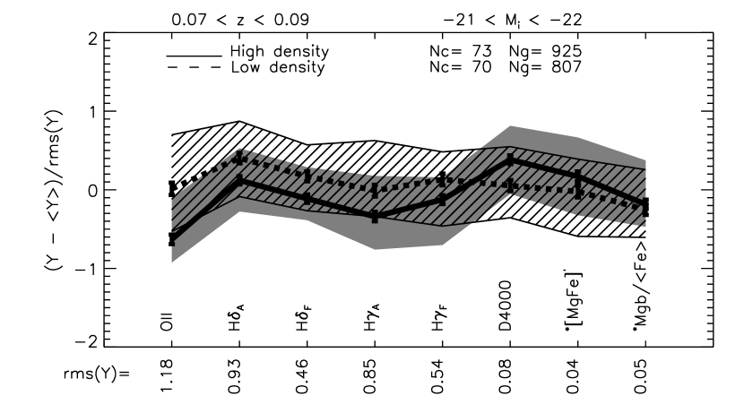
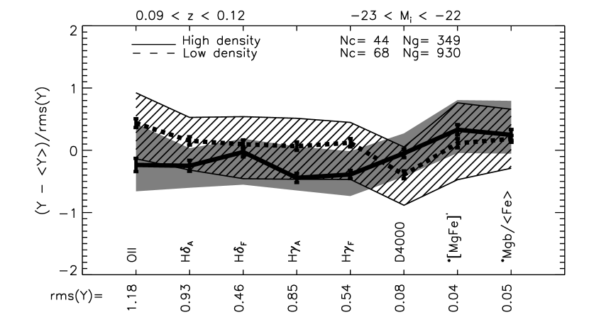
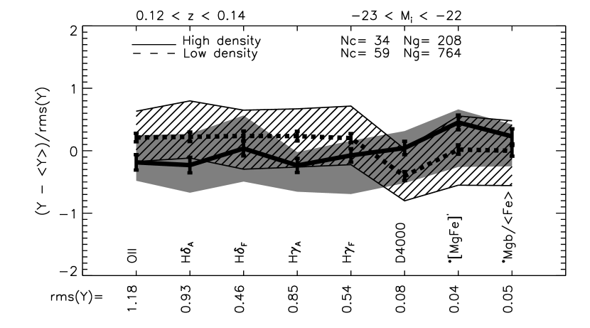
Figure 6: Emission line strengths (OII), star-formation indicators (H$\delta$, H$\gamma$), the strength of the break at 4000Å(D4000), and the combinations [MgFe]^′ and Mg/$\langle$Fe$\rangle$, for objects with the same narrow range of redshifts and luminosities as in the previous figure. An asterisk signifies that the quoted rms is for $\log_{10}$ of the index.

To simplify interpretation of the results, Figure 6 presents measurements in the same narrow bins in redshift and luminosity as were used in Figure 5. Recall that, for these bins, the effects of correlations between luminosity, velocity dispersion and environment are unimportant. (Plots similar to Figure 4 show similar trends to those in Figure 6, but are harder to interpret). Galaxies in low density regions have stronger emission lines, stronger Balmer lines, and weaker 4000Å breaks. They also tend to have lower values of [MgFe]^′ and Mg/$\langle$Fe$\rangle$. (KS tests indicate that the distributions are not significantly different if the small error bars shown for each parameter overlap.) In all observables, the high and low density samples differ by about three tickmarks, indicating that the difference is about 30% of the rms spread across the entire sample. Table 6 gives more precise values for these differences.

Recall that the mean luminosities and velocity dispersions are the same in dense and less dense environments. Therefore, trends with environment in Figure 6 are not the result of index-$\sigma$ and $\sigma$-environment correlations. We have already argued that these trends are probably not due to the morphology-density relation either.

4.3 Lick indices

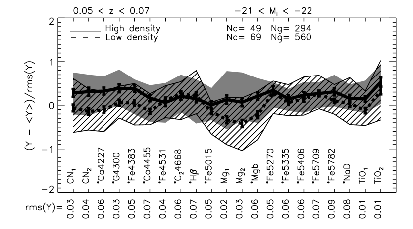
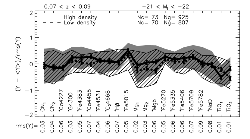
Figure 7: Lick indices for objects with the same narrow range of redshifts and luminosities as in the previous figure. (An asterisk signifies that the quoted rms is for $\log_{10}$ of the index.) Recall that the mean luminosity and velocity dispersions are the same in dense and less dense environments, so trends with environment are not caused by correlations with $\sigma$. Bottom panel contains a supercluster, so environmental effects may not be accurate.

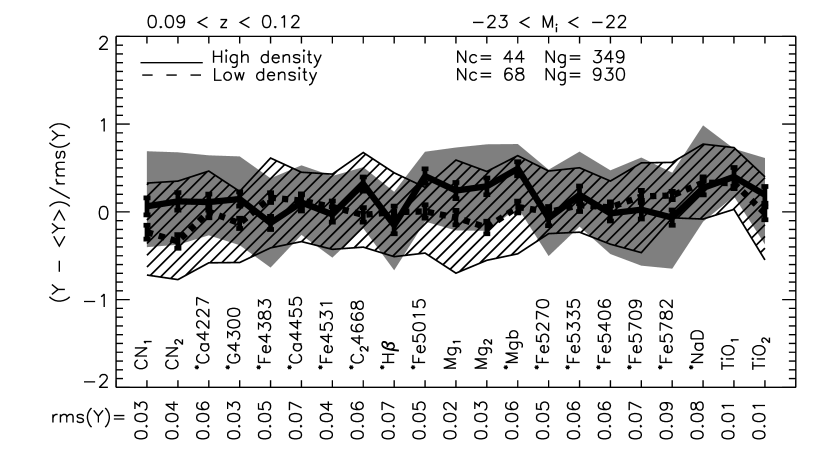
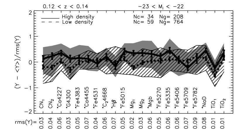
Figure 7: Continued.

Lick indices (defined as in Trager et al. 1998) for objects with the same narrow range of redshifts and luminosities as in the previous figure are shown in Figure 7. The indices are arranged in order of increasing wavelength, so the figure can be thought of as illustrating how (little) the spectrum depends on environment. Notice that the Mg line strengths tend to be slightly weaker in the low dense regions (about 30% of the rms across the full sample, making Mg₂ and Mg$b$ weaker by about $0.01\pm 0.004$ mags and $0.2\pm 0.06$ Å, respectively). On the other hand, most of the Fe indicators show no significant dependence on environment. Once again, KS tests indicate that the error bars provide a reasonably accurate guide to the significance of the difference between environments: overlapping error bars indicate no significant difference.

Table 6 quantifies the trends we have detected; recall that they are not the result of index-$\sigma$ and $\sigma$-environment correlations, and that they are unlikely to have arisen from a morphology-density relation. Presumably, age, metallicity and $\alpha$-element abundance differences play some role in the dependence on environment. By studying which indices behave similarly in these plots, one can begin to identify which elements respond similarly to variations in age, metallicity, and $\alpha$-abundance. We discuss this in the next section.

5 Evolution and environment

The previous section showed that, at any given redshift, many line strengths depend weakly, but significantly, on environment. On the other hand, many of the line strengths have evolved significantly between $z=0.05$ and $z=0.15$ (Bernardi et al. 2003d). Section 6 uses stellar population synthesis models to interpret our measurements. This section describes a relatively model independent interpretation of what our measurements mean.

5.1 Measurements of evolution

The luminosity function of this sample changes slightly with redshift (Bernardi et al. 2003b). The observed evolution can be accounted-for if one assumes that the number densities are not changing, but the higher redshift population is more luminous than that at lower redshifts: the change is $1.15z$, $0.85z$ and $0.75z$ in the $g$-, $r$- and $i$-bands. Since a pure luminosity evolution model is consistent with the data, it is plausible that the population at lower redshifts is a passively evolved sample of the population at higher redshifts. If so, then the observed evolution with redshift can be used as a clock. The argument is as follows.

The dashed lines in Figures 8–10 show how the structural parameters and line-strengths vary as the redshift changes. These dashed lines (the same in all four panels of each figure) represent the evolution of galaxies with $2.35\leq\log_{10}\sigma\leq 2.4$ over the redshift range $0.06\leq z\leq 0.17$. The actual values are reported in Table 6. (The redshift limits were set by requiring that these objects be seen over the entire redshift range, so as to minimize selection effects. Appendix A discusses why selection effects are important, why we chose this bin in $\sigma$, and why our estimates of evolution are almost certainly upper-limits.)

By using the same dashed curve in all four panels (note that the solid curves in the top two panels in each figure are for a lower luminosity bin), we are implicitly assuming that evolution is not differential (i.e., all galaxies evolve similarly). Since age is likely the main driver for the dependence on redshift, indices with similar values traced by the dashed line may have a similar fraction of the total scatter across the whole sample arising from changes in age. For reference, the range $0.06\leq z\leq 0.17$ corresponds to a time interval of $\sim 1.3$ Gyr.

Before we consider these figures in detail, recall that the Fundamental Plane indicates that galaxies in cluster-like environments are fainter than their counterparts in less dense regions (c.f. Table 5). Pure luminosity evolution between $0.06\leq z\leq 0.17$ gives approximately the same shift in magnitudes as those listed in Table 5 (e.g. in the $r$-band, the difference between environments is $\sim 0.08$ mags, and the evolution is $0.85\Delta z\sim 0.09$ mags). If the difference between the two environments is entirely due to age effects, then the objects in cluster-like environments must be older by 1.3 Gyrs. If the other structural parameters and line-strengths show environmental differences which are similar to those seen by comparing populations at redshifts which are separated by 1.3 Gyrs, then this would constrain the roles played by age and metallicity in determining environmental differences.

Figure 8 indicates that color is different from the other parameters such as size and velocity dispersion: 1.3 Gyrs of evolution appears to account for the entire spread in color values, but accounts for a negligible fraction of the spread in velocity dispersions, sizes and masses. Evidently, color responds very differently to age than do the other parameters. We discuss this in more detail shortly.

The dashed lines in Figure 9 indicate that the Balmer lines are weaker at low redshift, whereas D4000, [MgFe]^′ and Mg/$\langle{\rm Fe}\rangle$ are slightly stronger. The sign of the evolution is consistent with that of an aging single-burst population. Taken at face value, Figure 9 indicates that an age difference of 1.3 Gyrs can produce a change in the Balmer line strengths, and in D4000, which is almost as large as the rms spread across the whole sample. However, this apparently dramatic evolution should be treated cautiously. At low redshifts, the Balmer lines, and D4000, are close to the edge of the SDSS spectrograph where there are known to be flux-calibration problems at the 3% level. Evidence that this may have compromised our estimates of evolution is presented in Appendix B: the apparent evolution of H$\delta_{\rm A}+$H$\gamma_{\rm A}$ is about three times larger than measurements from the literature (Kelson et al. 2001) suggest. Hence, the dotted lines in Figure 9 show the result of dividing all estimates of evolution for the Balmer lines and D4000 by a factor of three. When this is done, 1.3 Gyrs of evolution produces a similar fraction of the rms spread ($\sim 30\%$) for OII, [MgFe]^′ and Mg/$\langle{\rm Fe}\rangle$. Note that this is a smaller fraction of the rms spread than it was for color.

The dashed lines in Figure 10 show that evolution accounts for different fractions of the rms spread across the sample for the different Lick indices. (We have again corrected for potential flux calibration problems by reducing the measured values, for indices with rest wavelengths shorter than 4350Å, by a factor of three: the dotted curves show these corrected values). For instance, an age difference of 1.3 Gyrs produces a change in Mg which is 50 percent of the spread in Mg line-strengths. If the spread in ages across the sample is 1.3 Gyrs, as color indicates, then we must conclude that other effects (such as metallicity) are responsible for the remaining scatter. Similarly, evolution changes the Fe index strengths by a negligible fraction of the spread in Fe index values (typically about 0.06 dex). Evidently, this spread must be due to effects other than (or in addition to) age. In this respect, our results indicate that Fe and Mg respond differently to age and metallicity, and that C₂4668 and NaD are more similar to Mg than to Fe.

Notice that H$\beta$ appears to evolve slightly less than the other Balmer lines shown in the previous figure. Although it is more sensitive to fill-in by emission than the other Balmer lines, we have attempted to correct for this (recall we add 0.05 OII to the measured value). Since emission is more likely in the higher redshift population, it may be that the deeping of the H$\beta$ absorption feature with redshift is compensated by fill-in due to emission, and our correction has not completely accounted for this.

5.2 Dependence on environment

The solid lines in Figures 8–10 show variations with environment. Each panel shows environmental differences for galaxies in small bins in luminosity and redshift (as indicated). Before we discuss individual parameters and indices further, notice how similar the solid curves are in each set of panels: environmental effects are approximately the same in all our redshift and luminosity bins (with the possible exception of the $z\sim 0.08$ bin which includes the supercluster). Table 6, which quantifies trends with redshift, also quantifies these enviromental trends.

Some of the differences between indices arise because the different observables correlate differently with luminosity (e.g. mass correlates more strongly with luminosity than size or velocity dispersion, and they all correlate more strongly with luminosity than does color). If an observable correlates strongly with luminosity, the rms spread reported along the bottom of each panel may be dominated by the rms spread in luminosities, rather than by the scatter at fixed luminosity (we discuss this again in the next section). The solid curves in the different panels show results for galaxies in a narrow bin in luminosity. In this case, even if age effects account for the full scatter in index strength at fixed luminosity, they will not account for the full (i.e., the one computed using the full range of luminosities) rms spread.

Previous work indicates that the slope of the color magnitude relation does not evolve out to redshifts of order unity, and this has been used to argue that residuals from the color magnitude relation are indicators of age (e.g. Kodama et al. 1998; Blakeslee et al. 2003). Since the various panels in Figure 8 are for a small range in luminosity, in essence, the value of the dashed line for color shows the mean color residual from the color magnitude relation. Hence, it is an age indicator. Since it shows the same variation as the solid line in the Figure (the difference between cluster and lower density environments), the mean age difference between environments is approximately the same as the mean age difference between the two indicated redshifts: on average, objects in dense regions are less than $\sim$1.3 Gyr older.

Like color, Mg shows approximately the same trends with environment as with redshift (Figure 10), although the magnitude of both trends for Mg appears to be approximately half that for color. However, Mg correlates strongly with luminosity, and a substantial part of this apparent difference is because we are only considering Mg for a small range in luminosity. If we account for this difference, then Mg and color are remarkably similar. If the age difference between cluster and low density environments is $\sim$1.3 Gyr, as suggested by color, then the similarity between the solid and dashed lines for Mg leaves little room for, e.g., metallicity effects. The next section provides a more quantitative model of these trends.

5.3 Interpretation: Evolution as a clock

The typical age, metallicity and $\alpha$-abundance may change with environment. If trends with redshift primarily reflect age effects, then a comparison of the dashed and solid lines allows one to constrain the relative roles of age and metallicity and/or $\alpha$-abundance on the different indices. A quantitative model is developed below.

Suppose that the spread in index strength $I$ is

$$\sigma^{2}_{II}(z)=\Bigl{[}f_{T}^{I}(z)\,\sigma_{T}(z)\Bigr{]}^{2}+\Bigl{[}f_{X}^{I}(z)\,\sigma_{X}(z)\Bigr{]}^{2}$$ (1)

where $T=\log_{10}$(age) and $X$ represents other effects (e.g., it could be $\log_{10}$(metallicity), $f_{T}^{I}$ describes how sensitive index $I$ is to age, $f_{X}^{I}$ describes how sensitive index $I$ is to other effects (e.g. metallicity), and $\sigma_{T}$ and $\sigma_{X}$ denote the spread in ages and the spread in everything else. Note that it is the combination $f_{T}\sigma_{T}$, rather than the two terms individually, which determines the contribution of age effects to the spread in index values. Also note that $\sigma_{T}$ and $\sigma_{X}$ are the same for all indices. (The expression above really follows from assuming that index strengths are determined by some, possibly degenerate, combination of age and other effects. For instance, if $X$ is mainly sensitive to metallicity, then the expression above is a consequence of the age-metallicity degeneracy. Models suggest that, in this case, $f_{X}/f_{T}=3/2$.)

If the only difference between the population at two redshifts is age, then the change in index strength is

$$\Delta I_{evol}=f_{T}^{I}\,\Delta T_{evol},$$ (2)

where $\Delta T$ denotes the change in $T$ between the two epochs. (This actually assumes that $f_{T}^{I}$ is the same for the two epochs, and that the other effects such as metallicity are also. This is unlikely to be correct if the age difference between the two epochs is large, so this really assumes that the two epochs are close in units of the timescale over which the relations between index strength and age and metallicity change.) This provides an estimate for $f_{I}^{T}$ in terms of observables.

Consider what this implies for color. It is often argued that residuals from the color magnitude relation are indicators of age. In such a model, the full spread in colors comes from the scatter in color at fixed magnitude, plus a term which accounts for additional effects:

$$\sigma_{CC}^{2}=\sigma_{C|M}^{2}+(f_{X}^{C}\sigma_{X})^{2}$$ (3)

Therefore,

$$f_{T}^{C}\sigma_{T} = \sigma_{C|M}\equiv\sigma_{CC}\sqrt{1-\xi_{CM}^{2}}\quad{\rm and}$$

$$f_{X}^{C}\sigma_{X} = \sqrt{\sigma_{CC}^{2}-\sigma_{C|M}^{2}}\equiv\sigma_{CC}\xi_{CM}.$$ (4)

(The previous section included a discussion of the relative roles of the scatter at fixed luminosity, and the slope of the index-luminosity relation. In the present context of the scatter in color, these are $\sigma_{C|M}$ and $\xi_{CM}\sigma_{CC}$: the scatter in colors at fixed magnitudes dominates if $|\xi_{CM}|\ll 1$.)

Since $\Delta C=f_{T}^{C}\,\Delta T$, $\sigma_{T}$ equals that $\Delta T$ for which $\Delta C=\sigma_{C|M}$. To illustrate, in the SDSS dataset studied in the main text, $\Delta C_{evol}=0.031$ when $\Delta T_{evol}$ corresponds to a time interval of 1.3 Gyrs. Therefore the time interval required to produce a color change of $\sigma_{C|M}$ is

$$\sigma_{T}=(\Delta T_{evol}/\Delta C_{evol})\,\sigma_{C|M}.$$ (5)

Since $\sigma_{C|M}$ is also measurable (the data indicate $\sigma_{C|M}=0.037$), one has calibrated the relation between age and color.

Now consider other indices. We observe a change $\Delta I_{evol}=f_{T}^{I}\,\Delta T_{evol}$, so, over the range $\sigma_{T}$, the change in index strength would have been

$$f_{T}^{I}\,\sigma_{T} = f_{T}^{I}\,\Delta T_{evol}\,(\sigma_{T}/\Delta T_{evol})=\Delta I_{evol}\,(\sigma_{T}/\Delta T_{evol})$$ (6)

$$= \Delta I_{evol}\,(\sigma_{C|M}/\Delta C_{evol}).$$

All the terms on the right hand side are observables, so $f_{T}^{I}\,\sigma_{T}$ can be estimated from the data. Since $f_{T}^{I}\,\sigma_{T}$ is the first term on the right hand side of equation (1), and the left hand side of equation (1) is also measured,

$$f_{X}^{I}\,\sigma_{X}=\sqrt{\sigma_{II}^{2}-\Delta I_{evol}^{2}\,(\sigma_{C|M}/\Delta C_{evol})^{2}}$$ (7)

can also be estimated from the data.

The relative importance of age to other effects on the distribution of index strengths is given by the ratio

$${f_{X}^{I}\sigma_{X}\over f_{T}^{I}\sigma_{T}} = \sqrt{\left({\sigma_{II}\over\Delta I_{evol}}{\Delta T_{evol}\over\sigma_{T}}\right)^{2}-1}$$ (8)

$$= \sqrt{\left(1.74{0.33\sigma_{II}\over\Delta I_{evol}}{\Delta C_{evol}/\sigma_{C|M}\over 0.031/0.037}\right)^{2}-1},$$

where the first line follows from equations (1) and (2), and the second line uses the fact that $\sigma_{C|M}/\Delta C_{evol}=\sigma_{T}/\Delta T_{evol}$ (equation 5), and writes everything in units of typical observed values (e.g., Mg, [MgFe’], D4000) all have $\Delta I_{evol}/\sigma_{II}\approx 0.4$). Since $\Delta T_{evol}/\sigma_{T}$ is the same for all indices, larger values of $\Delta I_{evol}/\sigma_{II}$ indicate that a larger fraction of the spread in index strengths comes from age-related effects. Thus, age determines a larger fraction of the observed spread in colors than it does for Mg, and ages matter even less for the spread in Fe values.

In addition to comparing the relative roles of age and other effects for a given index, we can also compare indices with one another. For instance, although $\sigma_{X}$ is not known, we know that it is the same for all indices $I$. Therefore, if we measure $\sigma_{II}^{2}-\Delta I_{evol}^{2}\,(\sigma_{C|M}/\Delta C_{evol})^{2}$ for two indices and compute the ratio, then the result equals the ratio of $(f_{X}^{I})^{2}$ for the two indices. This allows a calibration of the relative sensitivities of the two indices to effects included in $X$. Thus,

$${f_{X}^{{\rm Mg}b}\over f_{X}^{C}}={\sqrt{0.06^{2}-(0.020\,\sigma_{C|M}/0.031)^{2}\over\sigma_{CC}^{2}-\sigma_{C|M}^{2}}}=3.44,$$ (9)

whereas

$${f_{X}^{{\rm Mg}b}\over f_{X}^{\rm Fe}}=\sqrt{0.06^{2}-(0.020/0.031)^{2}\sigma_{C|M}^{2}\over 0.05^{2}-(0.005/0.031)^{2}\,\sigma_{C|M}^{2}}=1.11.$$ (10)

This indicates that color is less sensitive to effects such as metallicity than are Mg or Fe (or, e.g., metallicity and $\alpha$-enhancement effects on color cancel each other, whereas they do not cancel as strongly for Mg and Fe).

We can proceed further if we are willing to make more model-dependent assumptions. In models where residuals from the color-magnitude relation are age indicators, it is usually assumed that metallicity $\propto L^{\beta}$. Therefore, $\sigma_{Z}=0.4\beta\,\sigma_{MM}$, where $\sigma_{MM}$ denotes the rms spread in magnitudes. If $X$ is mainly sensitive to metallicity, then

$$f_{X}^{I}={2.5\over\beta}{\sigma_{CC}\over\sigma_{MM}}\,\sqrt{\left({\sigma_{II}\over\Delta I_{evol}}{\Delta C_{evol}\over\sigma_{CC}}\right)^{2}-1+\xi_{C|M}^{2}}.$$ (11)

If we set $\sigma_{CC}=0.04$, $\sigma_{MM}=0.71$, $\xi_{C|M}=0.4$, $\Delta C_{evol}=0.031$ and $\Delta I_{evol}/\sigma_{II}\approx 0.33$ (as it is for Mg, [MgFe]^′ and D4000), then

$${f_{X}^{I}\over f_{T}^{I}}={2.5\over\beta}{0.04\over 0.71}\,{2.16\over f_{T}^{I}}={0.30\over\beta}{\Delta T_{evol}\over\Delta C_{evol}}={0.44\over\beta}.$$ (12)

To obtain $f_{X}=(3/2)f_{T}$ as models suggest would require $\beta=0.3$: this is not inconsistent with single-burst models (e.g. Bruzual & Charlot 2003) of the color-magnitude relation (Bernardi et al. 2004). The implied spread in metallicity across the population is $\sigma_{Z}=0.4\beta\sigma_{MM}=0.08$.

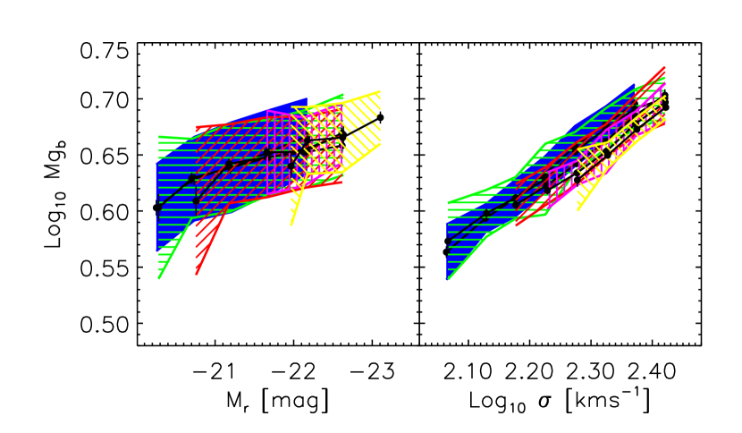
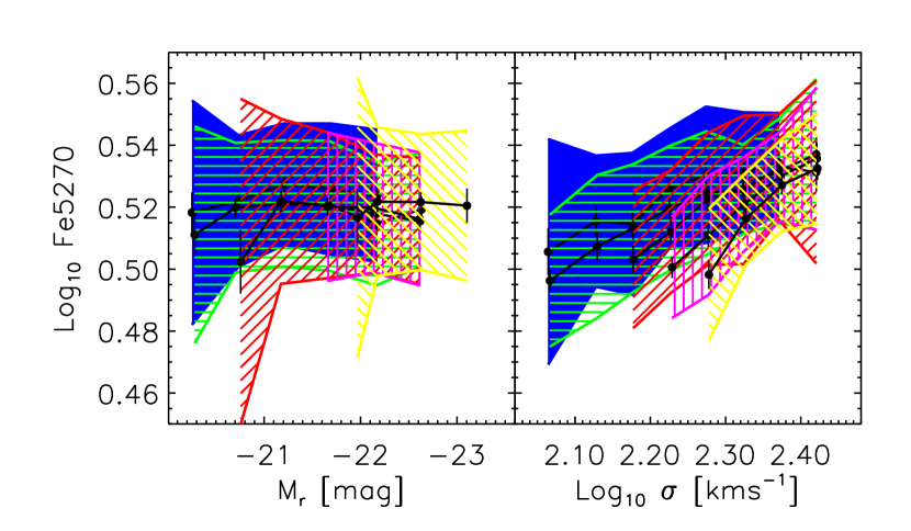
Figure 18: Top: correlation between Mg_b and magnitude (left panel) and velocity dispersion (right panel). Hashed regions show different redshift bins. Bottom: correlation between Fe5270 and magnitude (left panel) and velocity dispersion (right panel). The differential evolution see in the Fe-$\sigma$ relation is due to selection effects (see text for details).

The behaviour of Fe is difficult to explain in such a model. Figure 10 indicates that the trends with redshift and environment are weak. The lack of evolution is suggestive of Fe being sensitive to effects other than age. But if there is a metallicity-luminosity correlation, as suggested above, one would expect to see an Fe-luminosity correlation. There is no such correlation in our dataset (e.g., see Figure 18).

5.4 Comparison of evolution and environment

The previous subsection studied the effects of fixing the metallicity and varying the redshift by a small amount. Here, we fix the redshift and vary the environment. In this case,

$$\Delta I_{env}=f_{T}^{I}\sigma_{T}\,{\Delta T_{env}\over\sigma_{T}}+f_{X}^{I}\sigma_{X}\,{\Delta X_{env}\over\sigma_{X}}.$$ (13)

This illustrates that age differences can be compensated-for by associated changes in $X$.

Many of the indices have $\Delta I_{env}=\Delta I_{evol}$. In this case

$$f_{T}^{I}\,\Delta T_{evol}=f_{T}^{I}\sigma_{T}\,{\Delta T_{env}\over\sigma_{T}}+f_{X}^{I}\sigma_{X}\,{\Delta X_{env}\over\sigma_{X}},$$ (14)

so

$${\Delta T_{env}\over\sigma_{T}}={\Delta T_{evol}\over\sigma_{T}}-{f_{X}^{I}\sigma_{X}\over f_{T}^{I}\sigma_{T}}\,{\Delta X_{env}\over\sigma_{X}}.$$ (15)

If $\Delta X_{env}=0$, then the mean age difference between environments is the same as the mean age difference between two epochs, but in general, a larger or smaller age difference can be compensated-for by an associated change in $X$, and $(f_{X}\sigma_{X}/f_{T}\sigma_{T})$ governs how large this change must be.

For the indices where $\Delta I_{env}\approx\Delta I_{evol}\approx 0.33\sigma_{II}$ (e.g. Mg), $(\Delta T_{env}/\sigma_{T})=(\Delta T_{evol}/\sigma_{T})-1.42\,({\Delta X_{env}/\sigma_{X}})=0.84-1.42\,({\Delta X_{env}/\sigma_{X}})$; evidently, objects in the densest regions of our sample are older than those in the least dense regions, unless they have larger $X$ values (e.g., they are more metal rich) by $(0.84/1.42)\sigma_{X}$. Alternatively, if the objects in dense regions have smaller $X$ values (e.g., they are metal poor), then the age difference between environments can be larger than 0.84 times the rms age variation across the sample.

The age-$X$ degeneracy can be broken if we again consider color. Our estimate of environmental effects uses a small range of magnitudes in any given redshift bin, so, in effect, we are studying residuals from the color magnitude relation in different environments. If these residuals are only sensitive to age, they have $f_{X}^{C|M}=0$. Therefore, $\Delta T_{env}=\Delta C_{env}/f_{T}^{C|M}=\Delta C_{env}/(\Delta C_{evol}/\Delta T_{evol})$. It happens that $\Delta C_{env}\approx\Delta C_{evol}$, so $\Delta T_{env}\approx\Delta T_{evol}$. This age difference must be independent of the index which was used to estimate it. Now consider other indices for which $\Delta I_{env}\approx\Delta I_{evol}$ (e.g. Mg, Fe, D4000). Since equation (15) describes these indices, and $f_{X}^{I}\sigma_{X}/f_{T}^{I}\sigma_{T}$ is of order unity (equation 8), it must be that $\Delta X_{env}/\sigma_{X}\ll 1$.

The fact that Mg behaves similarly to color suggests that the entire environmental variation of Mg can be accounted for by age effects: metallicity effects are not very important. This leads to a provocative conclusion: claims that metallicity effects are important for explaining the weak environmental dependence of Lick index strengths like Mg are incompatible with currently popular interpretations of the color-magnitude relation.

6 Comparison with stellar population synthesis models

The previous section argued that our data are consistent with the hypotheses that the stellar populations of early-type galaxies in dense regions are slightly older than in less dense regions, and that metallicity differences between environments are negligible. This section shows that using single-burst stellar population synthesis models to interpret our data results in qualitatively similar conclusions.

6.1 The models

The models are characterized by three numbers: age, metallicity, and $\alpha$-enhancement. In most of the plots which follow, these models are evaluated on a grid of age = 2, 3, 5, 10 and 15 Gyrs, metallicity [Z/H] = $-0.33$, 0, 0.35 and 0.67, and [$\alpha/$Fe] = 0, 0.3 and 0.5, and we interpolate linearly between these grid points.

The effects of non-solar [$\alpha/$Fe] values have been considered by Tripico & Bell (1985), and incorporated into models by Trager et al. (2000), TMB03, TMK04 and Tantalo & Chiosi (2004). In what follows, we have chosen to concentrate on the models of TMB03-TMK04. However, the interpretations which follow are necessarily model dependent, and we caution that different models sometimes defer substantially from one another, so the resulting interpretations should be treated with caution. Indeed, Tantalo & Chiosi (2004) show that their $\alpha$-enhanced models can differ substantially from those of other groups, and have argued that uncertainties in how one treats [Ti/Fe] can have important effects. Hence, they argue strongly that the tendency to draw strong conclusions from such models is unwarranted.

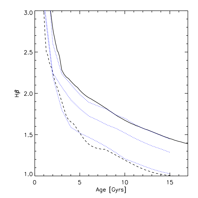
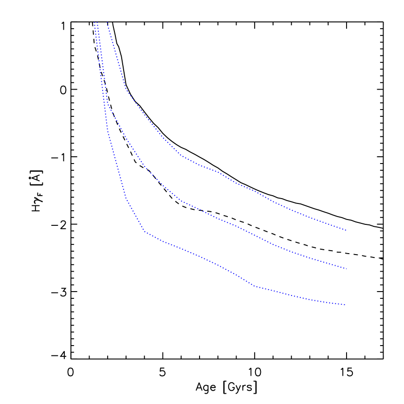
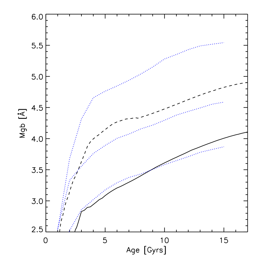
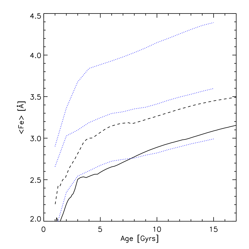
Figure 11: Evolution of various absorption line strengths in single burst stellar population synthesis models at solar $\alpha$-enhancement. Solid and dashed lines show the models of Bruzual & Charlot (2003) at solar metallicity and higher. Dotted lines show the models of TMB03-TMK04 at solar metallicity and higher. The models agree at solar metallicity (bottom curves in Mg$b$ and $\langle$Fe$\rangle$, top curves in H$\beta$ and H$\gamma_{\rm F}$), but, in general, do not agree at the higher metallicities which are expected to be characteristic of the early-type population.

To illustrate the point that all quantitative conclusions which follow are model dependent, Figure 11 compares the evolution of H$\beta$, H$\gamma_{\rm F}$, Mg$b$, and Fe, in the models of TMB03-TMK04 with the models of Bruzual & Charlot (2003). The model tracks are for solar [$\alpha$/Fe], because the Bruzual-Charlot models do not yet include non-solar [$\alpha$/Fe]. The solid and dashed curves in each panel show the Bruzual-Charlot models for two values of the metallicity (solar and greater than solar). The three dotted curves in each panel show the TMB03-TMK04 models for three different metallicities (solar and above, all at solar $\alpha$-enhancement). In all panels, the models agree at solar metallicity (the solid curve is close to the dotted one). However, in some panels the Bruzual-Charlot models are more like the highest metallicity TMB03-TMK04 models (e.g. H$\beta$), whereas in others, they are more like the intermediate metallicity models (e.g. H$\gamma_{\rm F}$).

To see that these differences matter, consider the two curves close to the center in the top right panel. Although the two models differ by 10 percent at fixed age, they differ by 100 percent at fixed $\langle$Fe$\rangle$. Since it is $\langle$Fe$\rangle$ which is observed, any quantitative conclusions about metallicity and age are strongly model dependent. The Figure also shows that the differences between the ages infered from the models will depend on whether one uses H$\beta$ or the higher-order Balmer lines H$\gamma_{\rm F}$, and that these differences can be substantial. The plot above suggests that one would infer younger ages from H$\gamma_{\rm F}$ than from H$\beta$, a point we will return to later.

6.2 The method

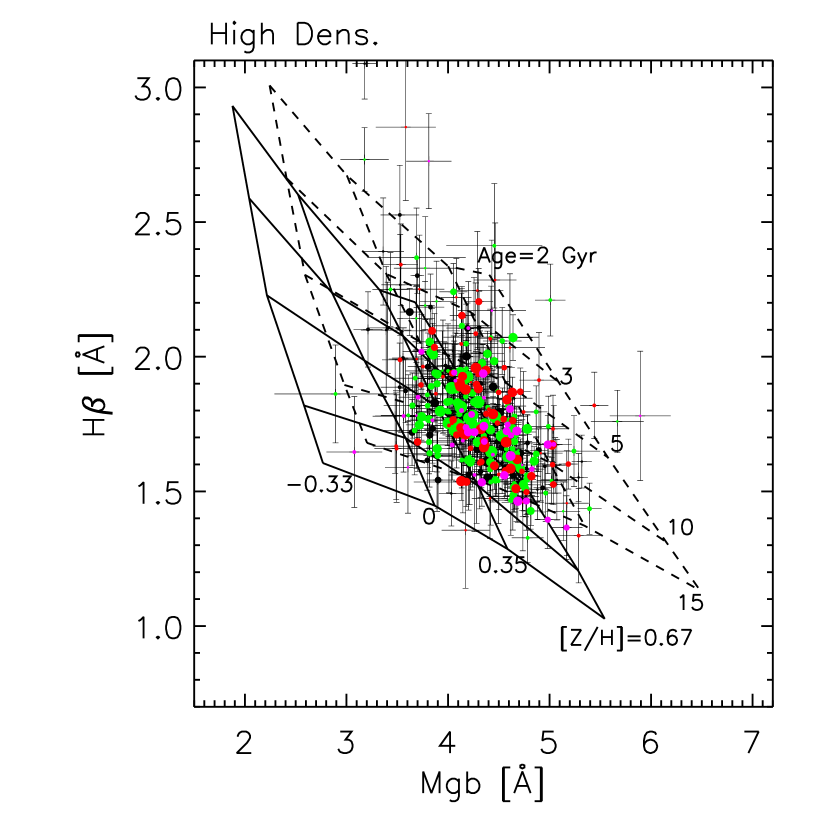
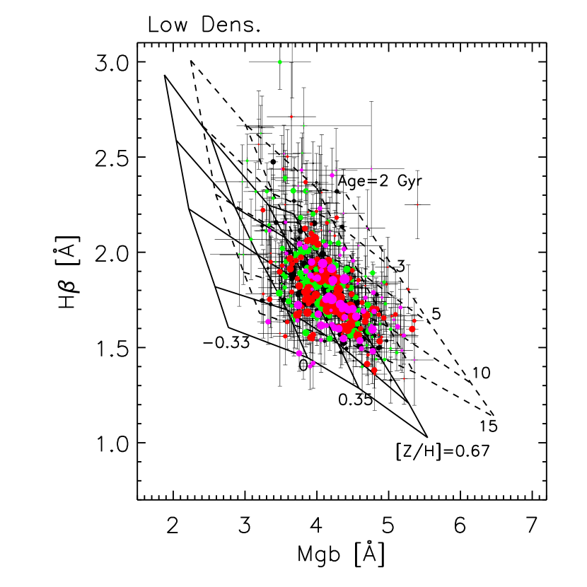
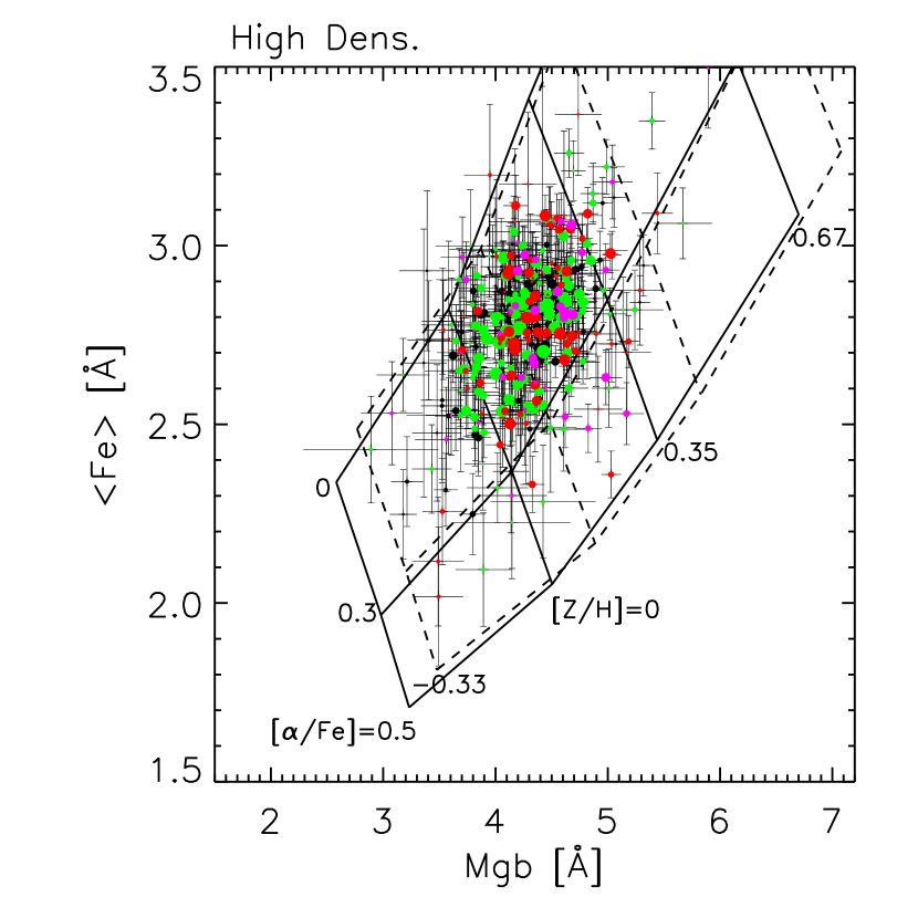
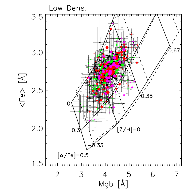
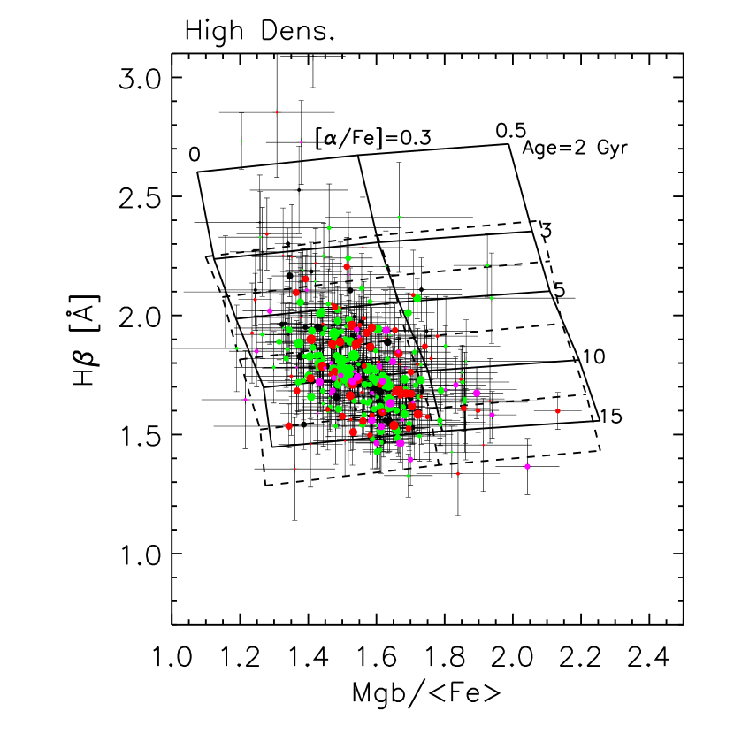
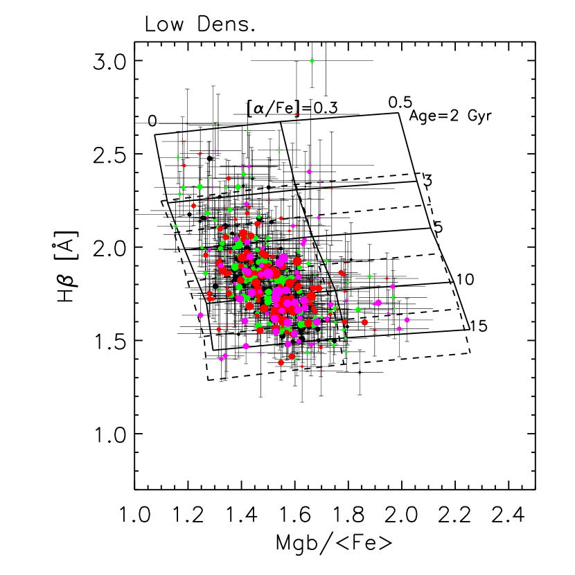
Figure 12: Distribution of H$\beta$ vs Mg (top), $\langle$Fe$\rangle$ vs. Mg (middle) and H$\beta$ vs Mg/$\langle$Fe$\rangle$ (bottom). Symbol sizes indicate the number of galaxies in the associated composite. Symbol colors indicate redshift: black, green, red and magenta points represent objects at $0.05<z<0.07$, $0.07\leq z<0.09$, $0.09\leq z<0.12$ and $0.12\leq z<0.14$. Grids show the models of TMB03. Solid and dashed grids show age and metallicity at $\alpha$-enhancements which are 0 (solar) and 0.3 (top panels), metallicity and $\alpha$-enhancement for ages of 10 and 15 Gyrs (middle panels), and ages and $\alpha$-enhancements when [Z/H] is 0 and 0.35 (bottom panels).

Figure 12 shows the distribution of H$\beta$ vs Mg (top), $\langle$Fe$\rangle$ vs. Mg (middle) and H$\beta$ vs Mg/$\langle$Fe$\rangle$ (bottom). Table 7 gives these index strengths at Lick, rather than SDSS, resolution. (Recall that $\langle$Fe$\rangle=$(Fe5270$+$Fe5335)$/2$.) In this, and the Figures which follow, we have divided the sample into the same small bins in redshift as in the previous figures, so as to be able to separate out the effects of evolution. Black, green, red and magenta points represent objects at successively higher redshifts ($0.05<z<0.07$, $0.07\leq z<0.09$, $0.09\leq z<0.12$ and $0.12\leq z<0.14$). In addition, symbol sizes have been scaled to reflect the number of galaxies which made-up the composites they represent.

The grids in each panel show the TMB03 models. The solid and dashed grids in the top panels show age and metallicity at $\alpha$-enhancements which are 0 (solar) and 0.3. This choice of observables separates out age and metallicity quite clearly. The observables in the middle panel separate out metallicity and $\alpha$-enhancement nicely: solid and dashed grids show metallicity and $\alpha$-enhancement for ages of 10 and 15 Gyrs. And the solid and dashed grids in the bottom panels show ages and $\alpha$-enhancements when the metallicity is solar and 0.35 respectively.

We determine ages, metallicities and $\alpha$-enhancements for each data point from these grids as follows. We begin with a guess for the $\alpha$-enhancement (say, solar). Then the H$\beta$-Mg plot provides estimates of the age and metallicity (by linear interpolation in the model grid). We then use the $\langle$Fe$\rangle$-Mg grid associated with the age estimate to estimate a metallicity and $\alpha$-enhancement. If this new $\alpha$-enhancement differs substantially from our initial guess, we return to the H$\beta$-Mg plot, but now use the new $\alpha$-enhancement to re-estimate the age and metallicity from the model, and use the new age estimate to determine the appropriate $\langle$Fe$\rangle$-Mg model with which to estimate [Z/H] and [$\alpha$/Fe] for the data point. We continue iterating this procedure until consistent ages, metallicities and $\alpha$-enhancements have been obtained. Typically, this happens after about five iterations. These provide our first estimates of self-consistent values of age, [Z/H] and [$\alpha$/Fe].

We then repeat this process, but now using the $\langle$Fe$\rangle$-Mg and H$\beta$-Mg/$\langle$Fe$\rangle$ plots. (I.e. we begin with a guess for the age, determine metallicity and $\alpha$-enhancement from the model grid for $\langle$Fe$\rangle$-Mg, and we use this metallicity to determine the model grid to use for the H$\beta$-Mg/$\langle$Fe$\rangle$ diagnostic. In turn, this provides revised estimates for the age and $\alpha$-enhancement; the new age estimate is then used in the $\langle$Fe$\rangle$-Mg diagram. This is repeated until a new self-consistent triple of age, [Z/H] and [$\alpha$/Fe] has been found.) Finally, we repeat all this using the H$\beta$-Mg/$\langle$Fe$\rangle$ and H$\beta$-Mg plots. Thus, we have three estimates of age, [Z/H] and [$\alpha$/Fe] which we can use to test for self-consistency (see next subsection).

It is particularly important to estimate the typical uncertainty on the derived parameters which are due to the measurement errors because the model grids are not aligned with the axes of observables in Figure 12, so these uncertainties will be correlated (e.g. Trager et al. 2000). We do this as follows. We compute the typical uncertainties in the measurements of H$\beta$, Mg and $\langle$Fe$\rangle$ (the errors on Mg/$\langle$Fe$\rangle$ are easily derived from those on Mg and $\langle$Fe$\rangle$). We then generate twenty seven mock ‘galaxies’ by adding and subtracting the reported measurement errors to the mean observed values of H$\beta$, Mg and $\langle$Fe$\rangle$, and hence Mg/$\langle$Fe$\rangle$ (we use mean, mean plus error, and mean minus error for each of the three observables). We then run the algorithm described in the previous section for each of these model ‘galaxies’. This provides three estimates of age, [Z/H] and [$\alpha$/Fe] for each of the twenty seven ‘objects’. The resulting distribution of points in the age, [Z/H] and [$\alpha$/Fe] plane forms our estimate of the full uncertainties in the derived parameters.

6.3 Results

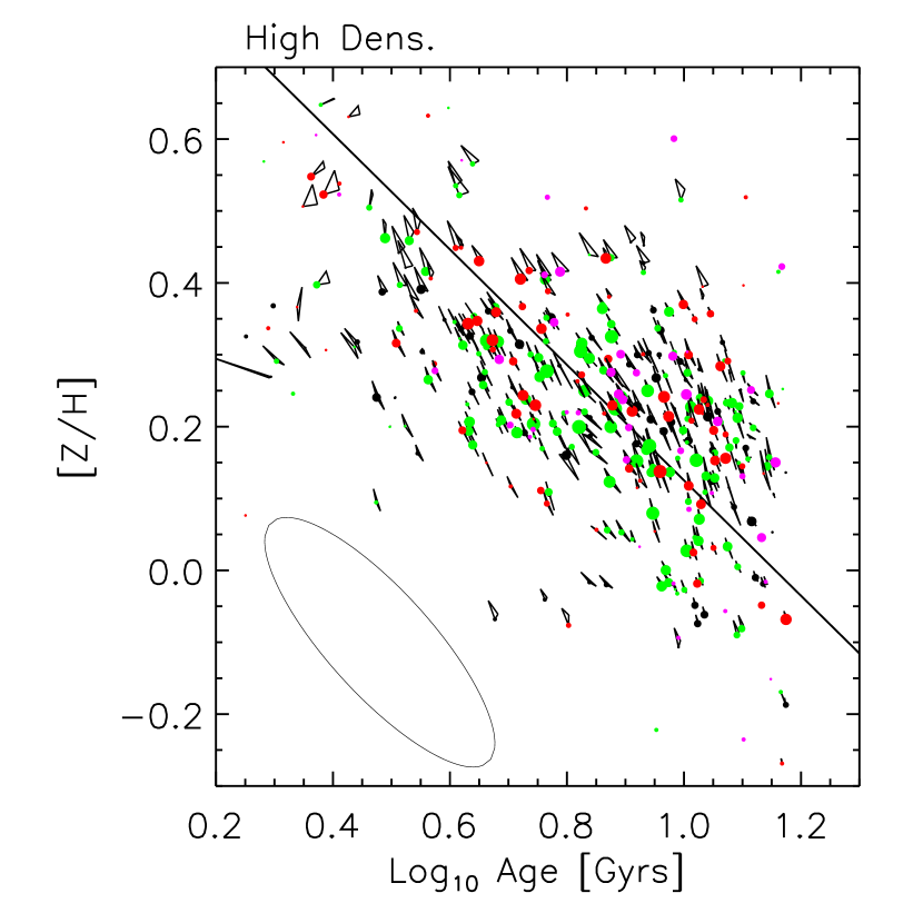
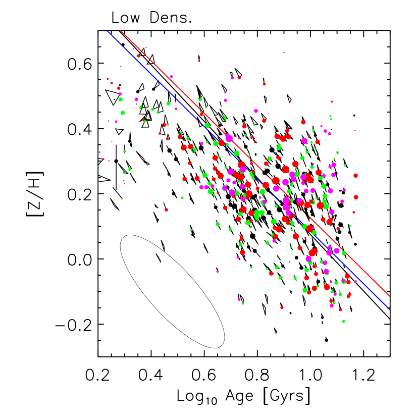
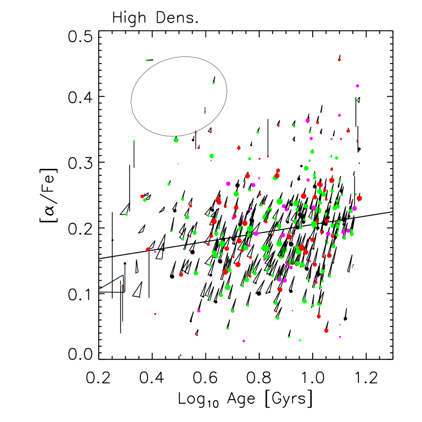
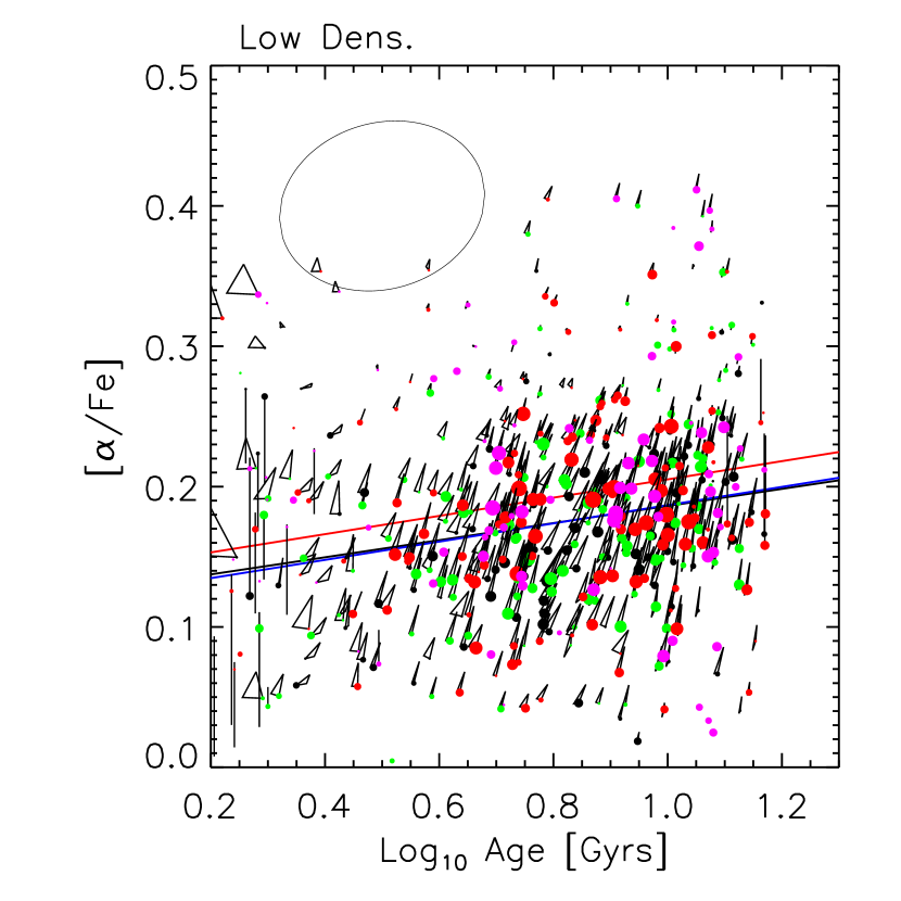
Figure 13: Pairwise correlations between derived ages, metallicities and $\alpha$-enhancements. The vertices of the triangle associated with each data point show the three estimates (see text) of each quantity; these provide a rough estimate of the systematic uncertainty in the derived quantities. The ellipse in the left-hand corner of each plot shows the typical uncertainty arising from the errors associated with measuring the line-indices. The shape of the ellipse in the top panels reflects the well-known degeneracy between age and metallicity. Solid lines in left panels show bisector (top left) and direct (bottom left) fits. Red and blue lines in the panels on the right compare the offset between high and low density environments if both samples are required to have the same slope as that shown in the left panel.

From the three combinations of plots described in the previous subsection, we have three different estimates of age, [Z/H] and [$\alpha$/Fe]. If the procedure just described is self-consistent, and the models are sufficiently realistic, one expects these three estimates to be similar. The extent to which this is the case is shown in Figure 13. Associated with each data point is a triangle, the vertices of which represent the three estimates of the derived age, [Z/H] and [$\alpha$/Fe]. The size of the triangle gives a rough estimate of the systematic uncertainty in the derived quantities associated with the model (i.e., assuming perfect measurements). The figure indicates that this uncertainty does not contribute significantly to the scatter in the various panels. Solid lines show the bisector fit to the relation in the top left panel, and the direct fit to the relation in the bottom panels. These suggest that older systems tend to have smaller metallicities (top panels) and slightly larger $\alpha$-enhancements (bottom panels).

The ellipses in the left corner of each panel show the typical uncertainty on the derived parameters which come from the measurement errors; these dwarf the systematic uncertainties associated with our algorithm. In the top panels especially, the errors are strongly correlated, so that much of the apparent anti-correlation between age and metallicity is due to the errors. This anti-correlation of the errors tracks the well-known age-metallicity degenaracy associated with such models. Table 8 provides the derived ages, [Z/H] and [$\alpha$/Fe] values, with associated error estimates, for each composite spectrum.

In all panels of Figure 13, the distribution of derived parameters is slightly, but not substantially, broadened by the errors. In particular, although the long-axis of the distribution shown in the top panels has been broadened by the correlated errors, the shape of the error ellipse shows that the distribution along the shorter axis cannot have been significantly broadened. Trager et al. (2000) argued that the scatter in this direction is primarily due to scatter in $\sigma$: objects with the same $\sigma$ lie parallel to this relation, with larger $\sigma$ objects lying at larger ages and metallicities. A similar statement applies if we substitute [$\alpha$/Fe] for $\sigma$. This is true of our dataset also: at fixed $\sigma$ (or [$\alpha$/Fe]), older objects appear to be metal poor.

The panels on the right allow a comparison between environments. Red lines show the fits from the panels on the left, and blue lines shows the result of fitting for the shift in zero-point while requiring the same slope as the red line. Black lines show the fit (bisector in top right panel, direct in bottom right) which allows the slope to vary as well. These fits indicate that there is a small offset between the age-metallicity correlation in the two environments, and that objects in dense regions tend to have slightly larger $\alpha$-enhancements than their counterparts of the same age in less dense regions.

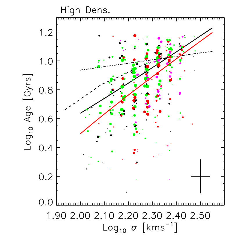
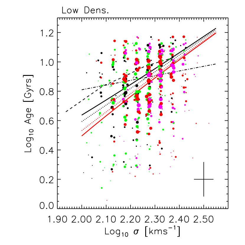
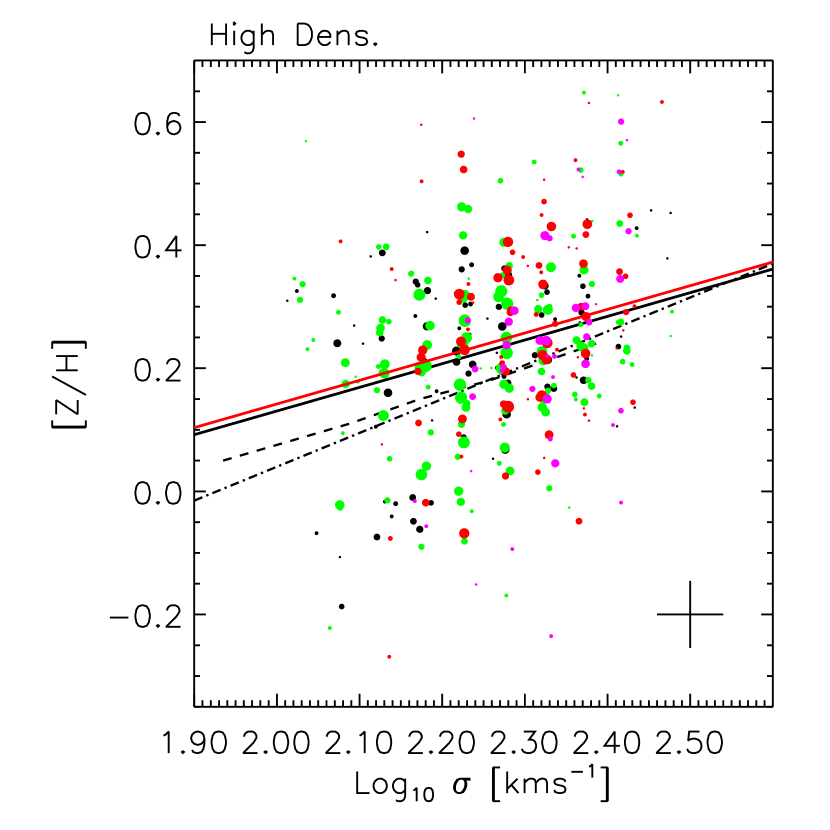
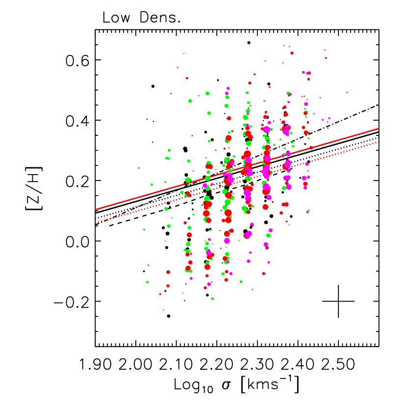
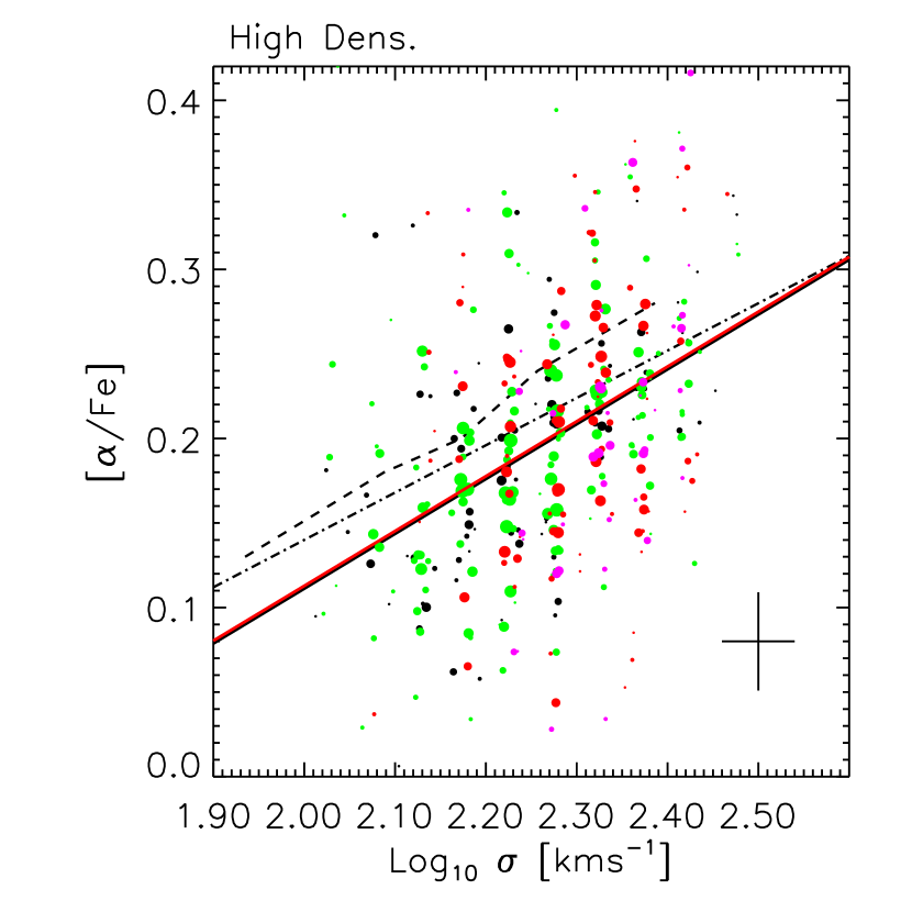
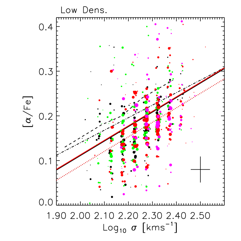
Figure 14: Objects with large $\sigma$ tend to be older (top panels), have larger metallicities (middle panels), and larger $\alpha$-enhancements (bottom). This is true at all redshifts in our sample: black lines show the mean relation at $z\sim 0.06$ and red lines show the result of fitting for the shift in Gyrs for the sample at $z\sim 0.11$. Moreover, note that there is clear evolution in the age-$\sigma$ relation, but not in [Z/H]-$\sigma$ or [$\alpha$/Fe]-$\sigma$. In addition, at fixed $\sigma$, objects in dense regions (solid lines) tend to have similar ages and metallicities as their counterparts in less dense regions (dotted lines in panels on right), and slightly larger $\alpha$-enhancements. Cross in the bottom right corner of each panel shows the typical uncertainty. Dashed and dot-dashed lines show the relations obtained by Nelan et al. 2005 and Thomas et al. (2005) in their analysis of other datasets.

Figure 14 shows all three derived quantities as a function of velocity dispersion in the two environments. (Because our three estimates of the derived quantities tend to be so similar, we have not shown the triangles associated with each point. Also, note the selection effect—the high redshift bins do not have objects at small $\sigma$). In each panel, black solid lines show direct fits to the relations in the high density regions at $z\sim 0.06$; red solid lines show the offset in Gyrs, [Z/H] and [$\alpha$/Fe] required to fit the relations at $z\sim 0.11$. Dotted lines in the panels on the right show the result of fitting for the offsets (in Gyrs, [Z/H] and [$\alpha$/Fe]) from the solid curves which best fit the relations for the low density sample. These fits show that, at any given redshift and in any environment, objects with large $\sigma$ tend to be older (top panels), have larger metallicities (middle panels), and larger $\alpha$-enhancements (bottom). These fits are given in Table 9, which also quantifies trends with redshift and environment.

Comparison of the red and black curves shows that the high and low density samples are both qualitatively consistent with the hypothesis of passively evolving populations: at fixed $\sigma$, the high redshift objects are younger, but there is no evolution in [Z/H] and [$\alpha$/Fe]. Moreover, the age difference is consistent with the redshift difference in our assumed cosmology.

Comparison of the solid and dotted lines in the panels on the right allows a study of the effects of environment. These indicate that, at fixed $\sigma$, objects in dense regions tend to have the same ages and metallicities as their counterparts in less dense regions, but they have slightly larger $\alpha$-enhancements. In constrast, Thomas et al. (2005) found that objects in less dense regions are slightly younger and metal rich, but they find no $\alpha$-enhancement effect (see also Kuntschner et al. 2001).

To study this further, dot-dashed lines show the fits reported by Thomas et al. (2005). Whereas our metallicity-$\sigma$ and [$\alpha$/Fe]-$\sigma$ values tend to be slightly different from theirs, our age-$\sigma$ relations are very different, especially in dense regions. On the other hand, our derived correlations in the high-density regions in are slightly better agreement with those of the NOAO-FP survey (Nelan et al. 2005) of clusters (dashed curves).

In the lower density regions, one might worry that our decision to compare low and high density environments by keeping the slope of the correlations with $\sigma$ fixed and simply fitting for an offset appears to be unreasonable for the [Z/H]-$\sigma$ relation. The slope of this relation appears to be steeper in the low density regions. Allowing for this would bring it into better agreement with that of Thomas et al. (2005). But the significant differences at high densities remain.

As a check, we have run our algorithm on the data analyzed by Thomas et al. (2005), and verified that the derived ages, metallicities and $\alpha$-enhancements we derive are within a few percent of those they obtained using a slightly different algorithm. For example, for an object with (H$\beta$, Mg $b$, $\langle$Fe$\rangle$) = (1.59Å, 4.73Å, 2.84Å), our procedure returns an age of 10.7 Gyr, [Z/H]=0.26 and [$\alpha$/Fe]=0.24. Thus, differences in our methods used to derive ages, [Z/H] and [$\alpha$/Fe] from the model grids are unimportant. Hence, we do not have a good explanation for why our correlations with $\sigma$, and the environmental dependences of these correlations, in our data set differ from the correlations in theirs—while our definitions of environment differ in detail, it is not obvious that this should lead to the relatively large qualitative differences we see.

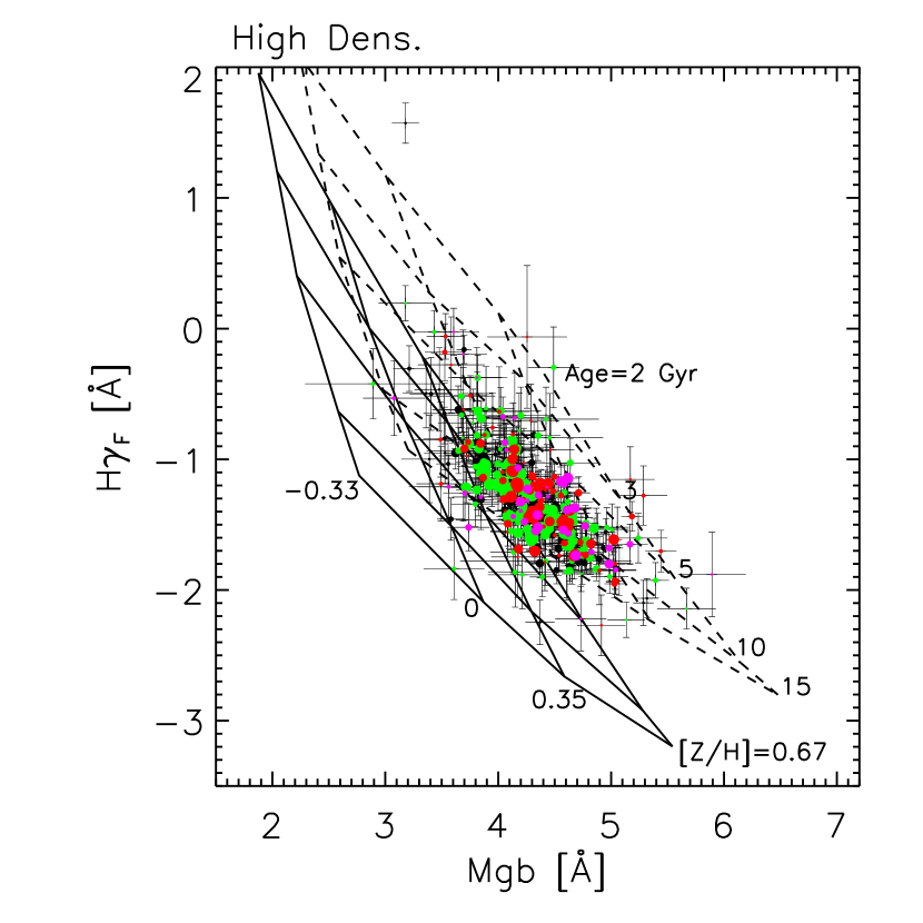
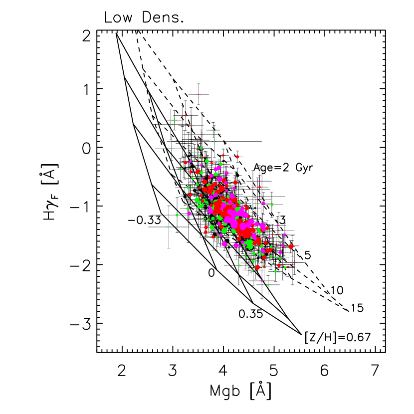
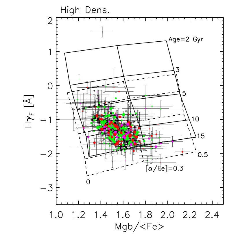
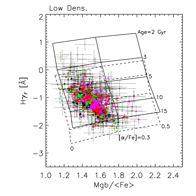
Figure 15: Same as Figure 12, but with H$\gamma_{\rm F}$ instead of H$\beta$. The top panel shows clearly that these objects have non-solar $\alpha$-element abundance ratios. (But see Appendix B for a discussion of whether flux calibration problems compromise the measurements in the lowest redshift bin.)

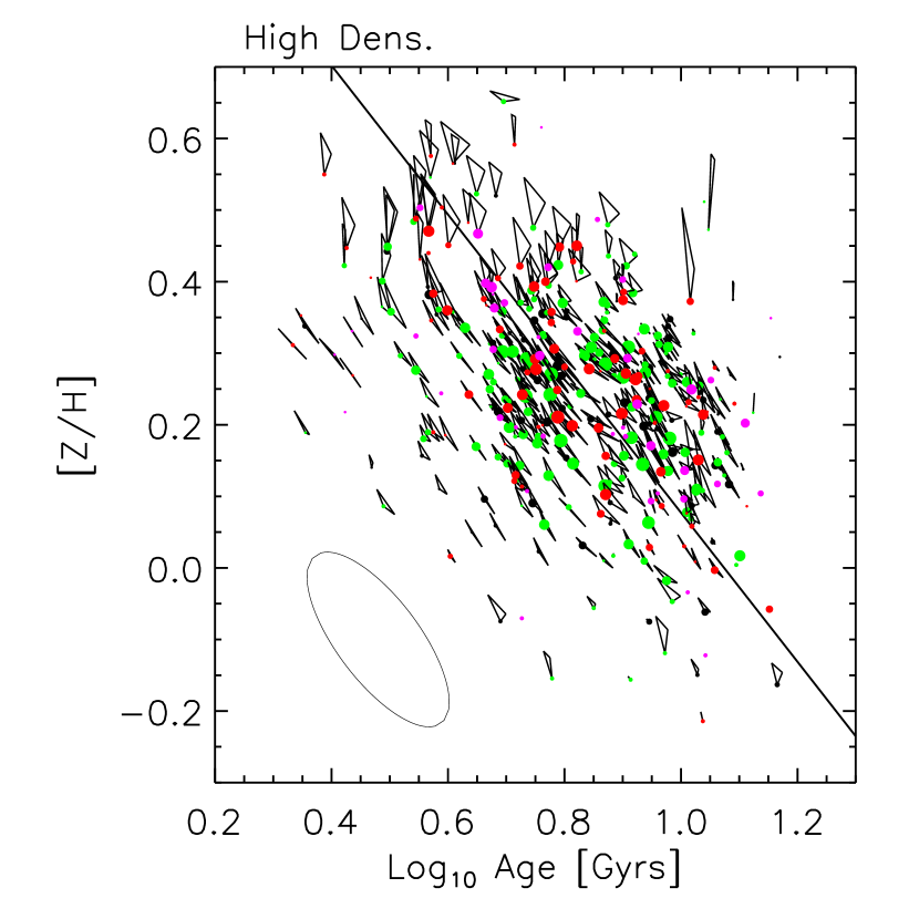
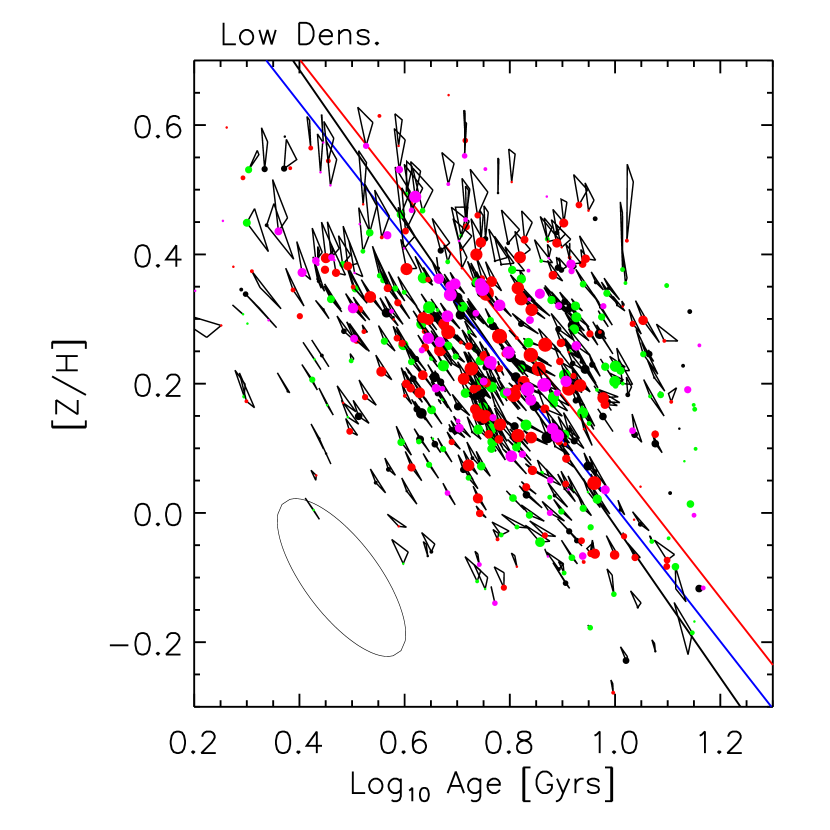
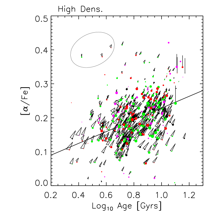
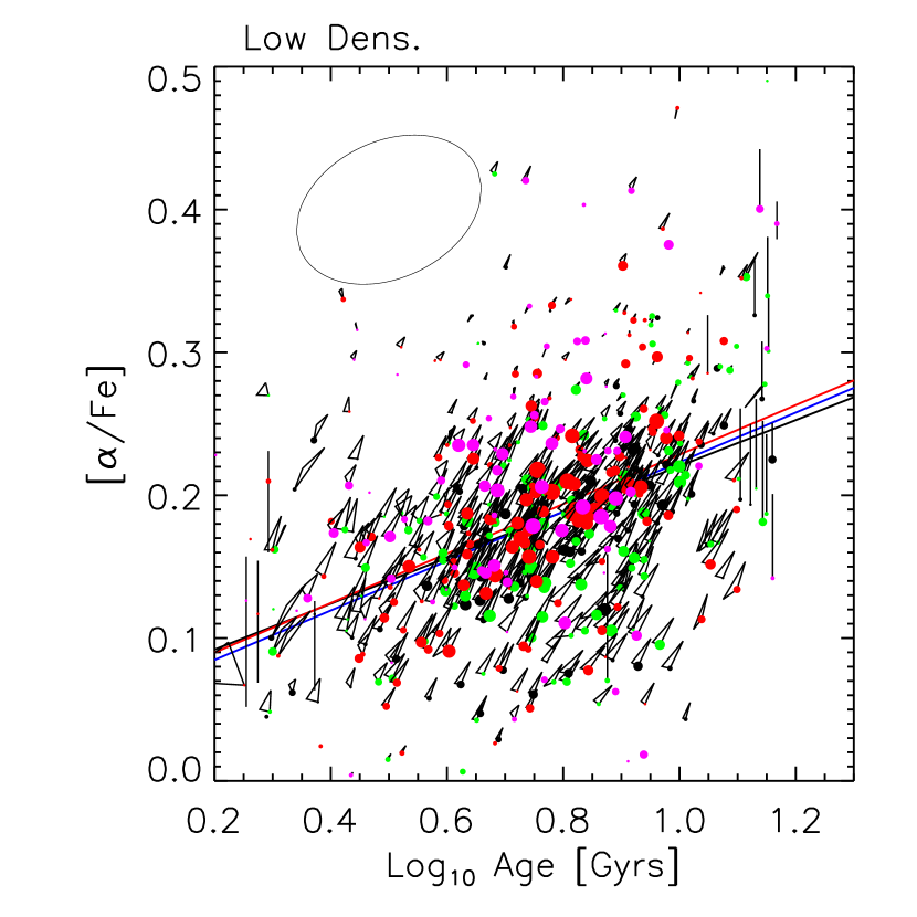
Figure 16: Same as Figure 13, but with H$\gamma_{\rm F}$ instead of H$\beta$. Here, the anti-correlation between [Z/H] and age is slightly steeper than before, and the correlation between [$\alpha$/Fe] and age is steeper and tighter than before. (See Appendix B for a discussion of whether flux calibration problems compromise the results in the lowest redshift bin.)

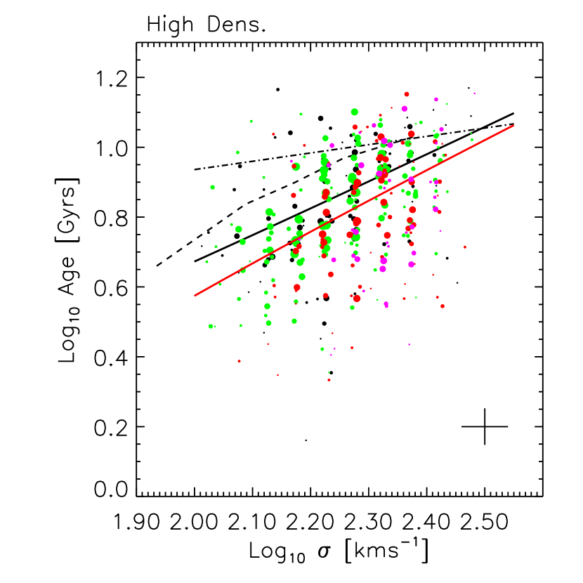
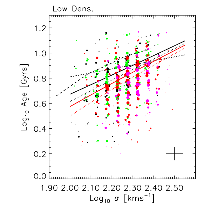
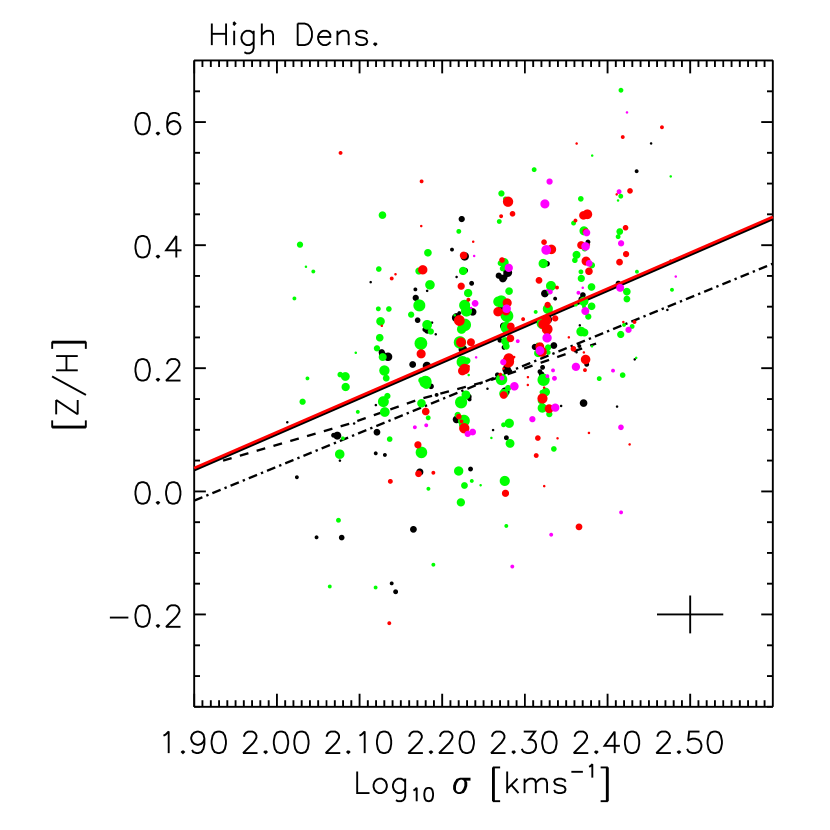
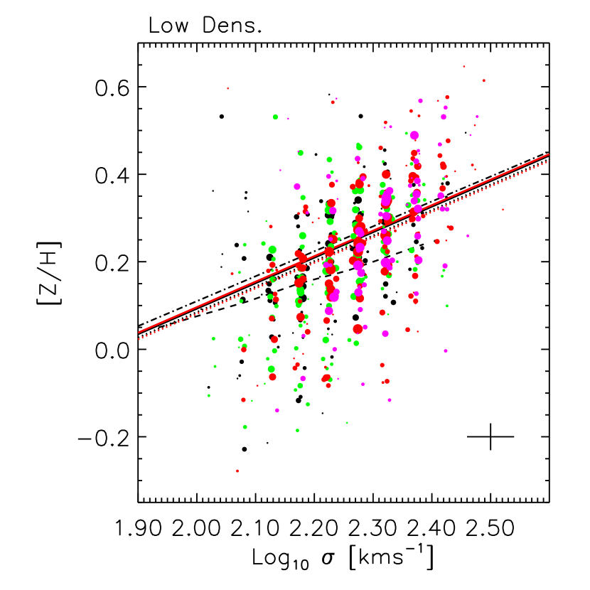
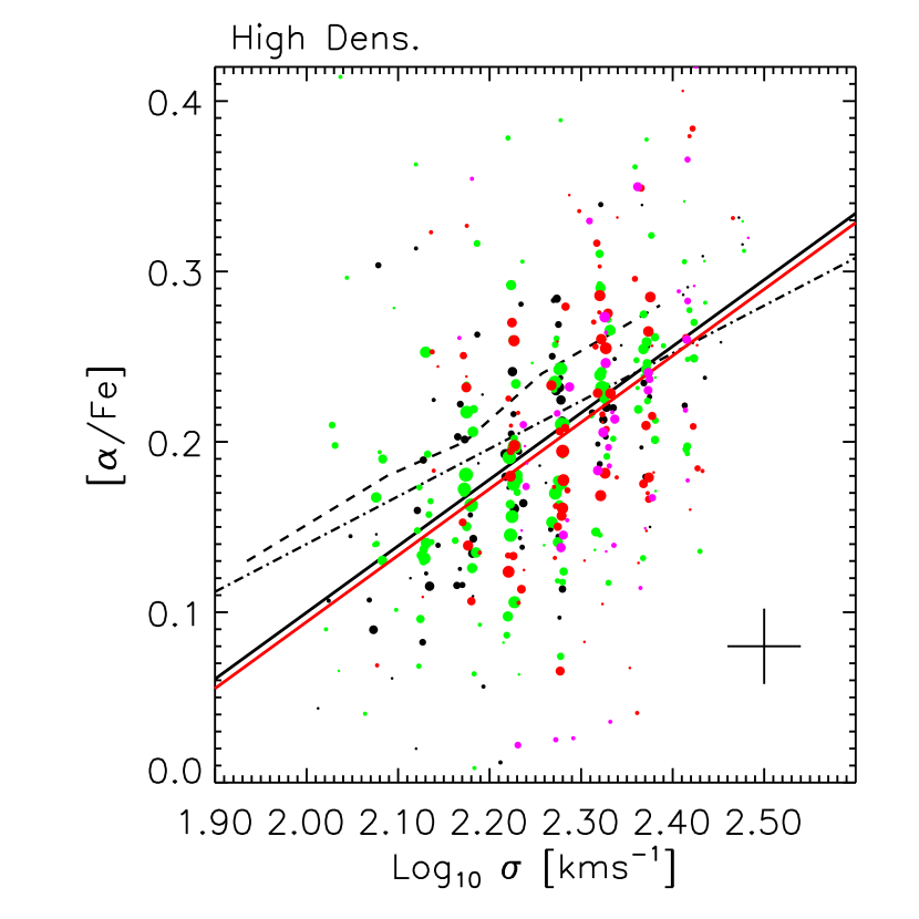
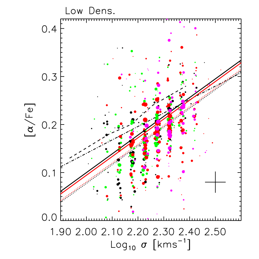
Figure 17: Same as Figure 14, but with H$\gamma_{\rm F}$ instead of H$\beta$. These panels show that the objects in the high redshift population (red lines) are younger than their counterparts of the same $\sigma$ at lower redshift (black lines). But there is no such trend for [Z/H] or [$\alpha$/Fe]. (But see Appendix B for a discussion of whether flux calibration problems compromise the results in the lowest redshift bin.) In addition, objects in lower density regions are slightly younger and less $\alpha$-enhanced than their counterparts in denser regions.

Figures 15–17 show the result of repeating this analysis but using H$\gamma_{\rm F}$ instead of H$\beta$. (This choice was motivated by discussion in TMK04; we find similar results if we use H$\delta_{\rm A}$+H$\gamma_{\rm A}$ instead.) In general, this choice results in ages that are younger by 1 Gyr, but similar [Z/H] and [$\alpha$/Fe]. This is true even if one allows for the possibility that there may be flux calibration problems for these Balmer lines at low redshifts (cf. Appendix B). (If there is a problem, then the ages we derive for the lowest redshift bin are overestimates, and the H$\gamma_{\rm F}$ ages will be even smaller than those from H$\beta$. In addition, the metallicities will increase slightly. Applying these corrections would make the relative differences between the low and high redshift samples, at least in dense regions, more similar to the differences seen when H$\beta$ was used. But the overall offsets between the ages and metallicities estimated from these two sets of plots remains. Note that this difference from the H$\beta$ results is what one might have guessed from the differences shown in Figure 11.) In particular, these differences are larger than any difference between the two environments.

7 Discussion and conclusions

The properties of early-type galaxies show weak but significant correlations with environment. The Fundamental Plane indicates that cluster galaxies are $\sim$0.08 mag/arcsec² fainter than their counterparts in low density environments, and the scatter around the plane shows no significant dependence on environment (Figure 3 and Table 5). This is consistent with the hypothesis that cluster galaxies are only slightly older than their counterparts in the low density environments, or that metallicity effects on the fundamental plane parameters counteract those of age.

Various indicators of chemical abundances also correlate weakly with environment: galaxies in low density environments are slightly bluer, have experienced star formation more recently, and have weaker D4000 and Mg (Figures 5–7), but these trends tend to be smaller than about 30% of the rms spread across the entire sample: i.e. the full distribution of observed values is not subtantially broadened by environmental effects.

Galaxy color, and many absorption line-indices, correlate primarily with velocity dispersion. However, differences between cluster and low density environment populations are seen even when the velocity dispersion is the same in both environments—the environment plays an important role in determining galaxy properties.

We discussed two methods of quantifying correlations with environment: both indicate that objects in clusters tend to be slightly older than those in less dense regions, but that metallicity differences are small. The first method (Section 5) uses an argument which is relatively model independent, and proceeds as follows. The absorption line-strengths evolve with redshift. Compared to their values at $z\sim 0$, Balmer lines were stronger, D4000 was weaker, Mg was weaker, and $\langle$Fe$\rangle$ was not very different at $z\sim 0.2$. If the high redshift population is simply a passively evolved version of that locally (previous analysis suggests that this is a good approximation), then the observed evolution with redshift can be used as a clock. In particular, comparison of the difference between cluster and low density environment populations with the dependence on redshift (Figures 8–10, and Table 6) allows one to constrain the different relative roles of age and metallicity/$\alpha$-abundance on the various observed properties of galaxies.

For instance, our analysis shows, in a model independent way, that Fe is less sensitive to age than is Mg. In addition, residuals from the Mg-luminosity relation show similar trends with evolution and environment as residuals from the color-magnitude relation. If we add the constraint that residuals from the color-magnitude relation are age indicators, then our data indicate that the rms spread in ages across the sample is slightly greater than $\sim 1.5$ Gyrs, and the rms spread in log₁₀(metallicity) is 0.08. In addition, galaxies in cluster environments are $\sim 1$ Gyrs older than their counterparts in less dense environments, and the metallicity difference between the two environments is a negligible fraction of the full range of metallicities in the sample.

The second method (Section 6) uses single burst stellar population synthesis models to interpret our data. These indicate that the objects at the lower redshifts in our sample are indeed consistent with being passively evolved versions of the objects at higher redshifts: we see evolution in age, but not in metallicity [Z/H] or the $\alpha$-element abundance ratio [$\alpha$/Fe]. We find that age, [Z/H] and [$\alpha$/Fe] all increase with increasing velocity dispersion $\sigma$, in qualitative agreement with previous work. In addition, objects in dense regions tend to be older by less than $1$ Gyr and have larger [$\alpha$/Fe] ($\sim 0.02$) than their counterparts of the same $\sigma$ in less dense regions, but there is no evidence that objects in low density regions are more metal rich (Figures 14 and 17). This suggests that, in dense regions, the stars in early-type galaxies formed at slightly earlier times, and on a slightly shorter timescale, than in less dense regions. This is in qualitative agreement with a number of recent results (e.g. Thomas et al. 2005; Carretero et al. 2004). Whereas these qualitative conclusions do not depend on which absorption lines are used to interpret the data, quantitative conclusions do: use of H$\beta$ leads to systematically older ages than does H$\gamma_{\rm F}$.

We began with the statement that the monolithic and stochastic models make different predictions for how early-type galaxy properties should depend on environment. While the analyses presented here do not answer the question of which model is correct, we feel that they provide a useful method for addressing this issue. In particular, it will be interesting to see if these models are able to reproduce the weak environmental dependence of formation time and timescale suggested by our data.

Funding for the creation and distribution of the SDSS Archive has been provided by the Alfred P. Sloan Foundation, the Participating Institutions, the National Aeronautics and Space Administration, the National Science Foundation, the U.S. Department of Energy, the Japanese Monbukagakusho, and the Max Planck Society. The SDSS Web site is http://www.sdss.org/.

The SDSS is managed by the Astrophysical Research Consortium (ARC) for the Participating Institutions. The Participating Institutions are The University of Chicago, Fermilab, the Institute for Advanced Study, the Japan Participation Group, The Johns Hopkins University, the Korean Scientist Group, Los Alamos National Laboratory, the Max-Planck-Institute for Astronomy (MPIA), the Max-Planck-Institute for Astrophysics (MPA), New Mexico State University, University of Pittsburgh, Princeton University, the United States Naval Observatory, and the University of Washington.

Appendix A Evolution and selection effects

In the main text, we present estimates of how index-strengths in the population have evolved. In all cases, these estimates were made by computing residuals from the index-$\sigma$ relation rather than from the index-magnitude relation. This was done for two reasons. First, for almost all indices, the index-$\sigma$ relation is considerably tighter than the index-luminosity relation, so a small amount of evolution is more easily detected. Second, the velocity dispersion is expected to evolve much less than the luminosity, so it is a more direct surrogate for estimating evolution at fixed mass.

However, the SDSS sample is magnitude limited. Therefore, care must be taken to account for the effects of this selection before interpretting trends with redshift as being due to evolution. To illustrate, Figure 18 shows the Mg-luminosity, Mg-$\sigma$, Fe-luminosity and Fe-$\sigma$ correlations measured using objects in different redshift bins (bins are adjacent with edges at $z=0.05$, 0.07, 0.09, 0.12, 0.14 and 0.17, as in the main text). The plot uses luminosities corrected for evolution to $z=0$. In all cases, the filled circles show the median values of the index (Mg or Fe) in small bins in luminosity or $\sigma$. Hashed regions show the range which includes sixty-eight percent of the objects. (Mg and Fe are representative of most of the other indices presented in the main text.)

At any given redshift, Mg correlates with both luminosity and $\sigma$ whereas Fe correlates with $\sigma$ but not with luminosity. The Mg-$\sigma$ correlation is significantly tighter than Mg-luminosity. Both Mg-$\sigma$ and Fe-$\sigma$ appear to evolve. In the case of Fe-$\sigma$, the apparent evolution is differential. One might have thought that because Fe does not correlate with luminosity, measurement of the Fe-$\sigma$ relation can be made without worrying about the magnitude limit of the sample, so the differential evolution is real. The following model shows that this is not the case.

Let $I_{*}$, $M_{*}$ and $V_{*}$ and $\sigma_{II}$, $\sigma_{MM}$ and $\sigma_{VV}$ denote the mean and rms values of index strength, absolute magnitude and log₁₀(velocity dispersion) in the entire population at a given redshift (i.e., not just the part which was selected for observation). Let ${\cal I}=(I-I_{*})/\sigma_{II}$, ${\cal M}=(M-M_{*})/\sigma_{MM}$, and ${\cal V}=(V-V_{*})/\sigma_{VV}$ and define $\xi_{IM}\equiv\langle{\cal I}{\cal M}\rangle$, $\xi_{IV}\equiv\langle{\cal I}{\cal V}\rangle$, and $\xi_{VM}\equiv\langle{\cal V}{\cal M}\rangle$, where the angle brackets denote averages over the entire population. The mean value of $I$ at fixed $M$ is

$$\langle{\cal I}|{\cal M}\rangle={\cal M}\,\xi_{IM},\quad$$ (A1)

and similar expressions hold for the other pairs of observables: e.g. $\langle{\cal I}|{\cal V}\rangle={\cal V}\,\xi_{IV}$, $\langle{\cal V}|{\cal M}\rangle={\cal M}\,\xi_{VM}$, $\langle{\cal M}|{\cal I}\rangle={\cal I}\,\xi_{IM}$, etc. Similarly, the mean $I$ at fixed $V$ and $M$ is

$$\left\langle{\cal I}\Big{|}{\cal M},{\cal V}\right\rangle = {\cal M}\,{\xi_{IM}-\xi_{IV}\xi_{MV}\over 1-\xi_{MV}^{2}}$$ (A2)

$$+\ {\cal V}\,{\xi_{IV}-\xi_{IM}\xi_{MV}\over 1-\xi_{MV}^{2}}$$

with obvious permutations giving $\langle{\cal M}|{\cal V},{\cal I}\rangle$ and $\langle{\cal V}|{\cal I},{\cal M}\rangle$.

If the correlation between index and magnitude is entirely due to the index-$\sigma$ and magnitude-$\sigma$ correlations, then $\xi_{IM}=\xi_{IV}\xi_{VM}$. (Bernardi et al. 2004 show that this is true for the color-$\sigma$ relation.) In this case, $\langle{\cal I}|{\cal M},{\cal V}\rangle={\cal V}\,\xi_{IV}$ is independent of ${\cal M}$, so the index-$\sigma$ relation can be measured directly from the observed data without worrying about the magnitude limit (e.g. Bernardi et al. 2004). Note that this is despite the fact that there is an index-magnitude relation.

Now consider what happens if the index does not correlate with magnitude (as is the case for Fe): $\xi_{IM}=0$. In this case, $\langle{\cal I}|{\cal M},{\cal V}\rangle=({\cal V}-\xi_{MV}{\cal M})\,\xi_{IV}/(1-\xi_{MV}^{2})$. Because this expression depends on absolute magnitude, measuring the mean index strength as a function of velocity dispersion using galaxies observed in a fixed redshift bin of a magnitude limited sample will lead to a biased estimate of the true correlation.

To illustrate this bias, a mock galaxy catalog was generated by distributing objects uniformly in a comoving volume with $p(M,V,I)$ a multivariate Gaussian. The parameters of this Gaussian were chosen to match the distribution of luminosities and velocity dispersions in the catalog (from Bernardi et al. 2003b): $\sigma_{MM}=0.84$, $\sigma_{VV}=0.11$, $\xi_{MV}=-0.77$, $\sigma_{II}=0.05$ and $\xi_{IV}=0.25$. (The values of $\sigma_{II}$ and $\xi_{IV}$ were chosen to match the Fe-$\sigma$ relation.)

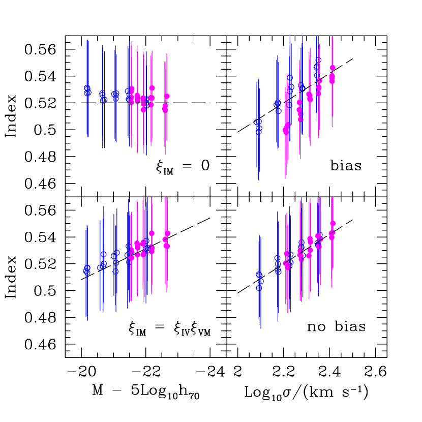
Figure 19: Index-luminosity and index-$\sigma$ relations measured from a magnitude limited catalog in low (open circles) and high-$z$ bins (filled circles). Error bars show the values at the 25th and 75th percentile. Dashed lines show the true relations. Top panel shows a model in which index strength does not correlate with magnitude, and bottom panel shows a model in which the index-magnitude correlation is entirely due to the index-$\sigma$ and magnitude-$\sigma$ correlations. Note the bias in the top right panel, which appears to indicate differential evolution.

The top set of panels in Figure 19 shows the index-magnitude and index-$\sigma$ relations if $\xi_{IM}=0$. Dashed lines show the input relations, and symbols show the relations measured using objects which have apparent magnitudes between 14.5 and 17.45 but have redshifts between 0.05 and 0.07 (open circles) or 0.12 and 0.14 (filled circles). Different sets of symbols at each bin are for different realizations of mock catalogs which have approximately the same number of objects in each redshift bin as the data ($\sim 1500$ for the redshift bins shown). The apparent steepening of the index-$\sigma$ relation with redshift is entirely due to the magnitude limit. This demonstrates that direct measurement of the index-$\sigma$ using objects in an apparent magnitude limited catalog can lead to a biased estimate of the true relation, even if the index itself does not correlate with absolute magnitude.

The bottom panel is similar, except that it has $\xi_{IM}=\xi_{IV}\xi_{VM}$. In this case, the index-luminosity and index-$\sigma$ relations measured in the magnitude limited sample are unbiased estimates of the true relation, even though index-strength correlates with magnitude—in agreement with the model described above.

Thus, for the Fe-$\sigma$ relation in Figure 18, most of the difference between the low and high-redshift bins is a selection effect. The Mg-luminosity correlation is slightly weaker than $\xi_{IV}\xi_{VM}$, so it too is biased by selection effects, although by a smaller amount. In all cases, the selection effect is more dramatic at low $\sigma$. Since we are interested in estimating how these indices evolve, we estimate evolution from the highest bin in $\sigma$ for which we have at least 1000 objects over $0.06\leq z\leq 0.17$: i.e., $2.35\leq\sigma\leq 2.4$. Since even this may be slightly affected by selection effects, it gives an upper limit to the true evolution.

Appendix B SDSS flux-calibration and Balmer line-strengths

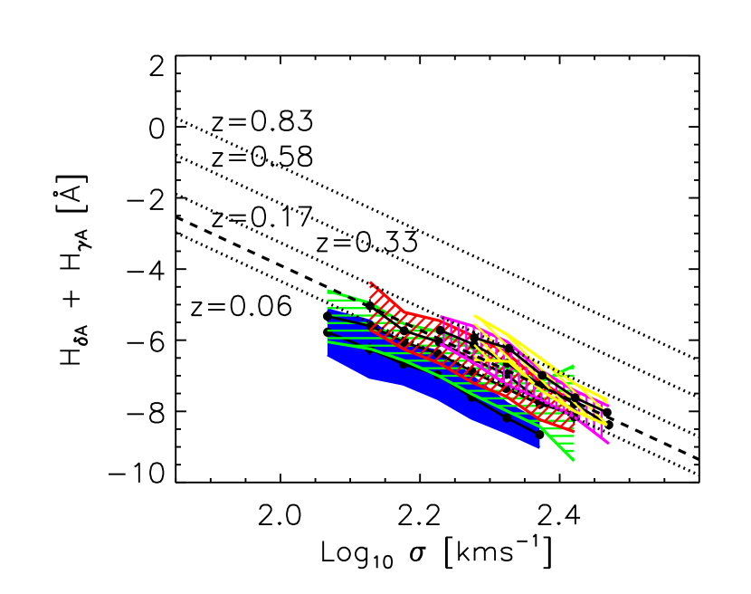
Figure 20: Comparison of the correlation between (H$\delta_{\rm A}+$H$\gamma_{\rm A}$) and velocity dispersion in our sample (shaded regions show different redshift bins) with the relation measured using galaxies in clusters at redshifts $z=0.06$, 0.33, 0.58 and 0.83 (dotted lines, from Kelson et al. 2001). Dashed line shows the relation obtained by interpolating between the 0.06 and 0.33 lines to $z=0.17$ for ease of comparison with our data. While the SDSS data have the same slope, they have a smaller zero-point at low redshift. Thus, the apparent evolution in the SDSS sample is about a factor of three larger than indicated by the dotted lines.

The main text notes that flux calibration problems around 4000Å may affect measurements of Balmer line-strengths and D4000. Evidence that this is a serious concern is presented in Figure 20. Dotted lines show the correlation between H$\delta_{\rm A}+$H$\gamma_{\rm A}$ and velocity dispersion measured by Kelson et al. (2001) using early-type galaxies in four clusters at the redshifts indicated. They find that the zero point of the relation evolves, but are not able to conclude if the slope does or not.

The shaded regions show the correlation between H$\delta_{\rm A}$+H$\gamma_{\rm A}$ and velocity dispersion in our sample in the same redshift bins used in the main text ($0.05<z<0.07$, $0.07<z<0.09$, $0.09<z<0.12$, $0.12<z<0.14$ and $0.14<z<0.20$). Notice that our SDSS data produce the same slope as the data from the literature, but the zero points are quite different at low redshift.

What is most relevant to the analysis in the main text is the rate at which the line strengths evolve. Since flux-calibration problems affect observed wavelengths, they appear as redshift dependent effects when studying features at fixed restframe wavelength. Figure 20 demostrates that the apparent evolution in the SDSS sample is about three times larger than that seen by Kelson et al. (2001). Since we already have reason to believe that flux-calibration is difficult around $\lambda_{obs}=4000$Å, so it is possible that the low redshift bins are more strongly affected than the bins at higher redshift, this strongly suggests that flux calibration systematics are affecting the SDSS measurement. Therefore, in the main text, we show the apparent evolution using the raw measurements as well as the result of dividing the apparent evolution by a factor of three.

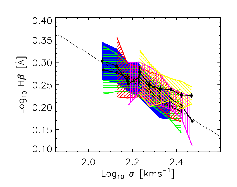
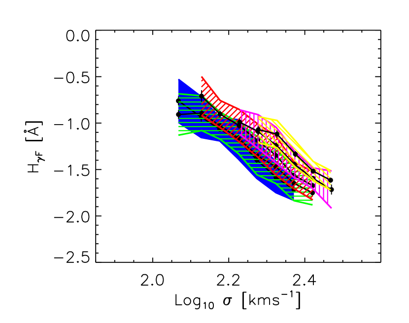
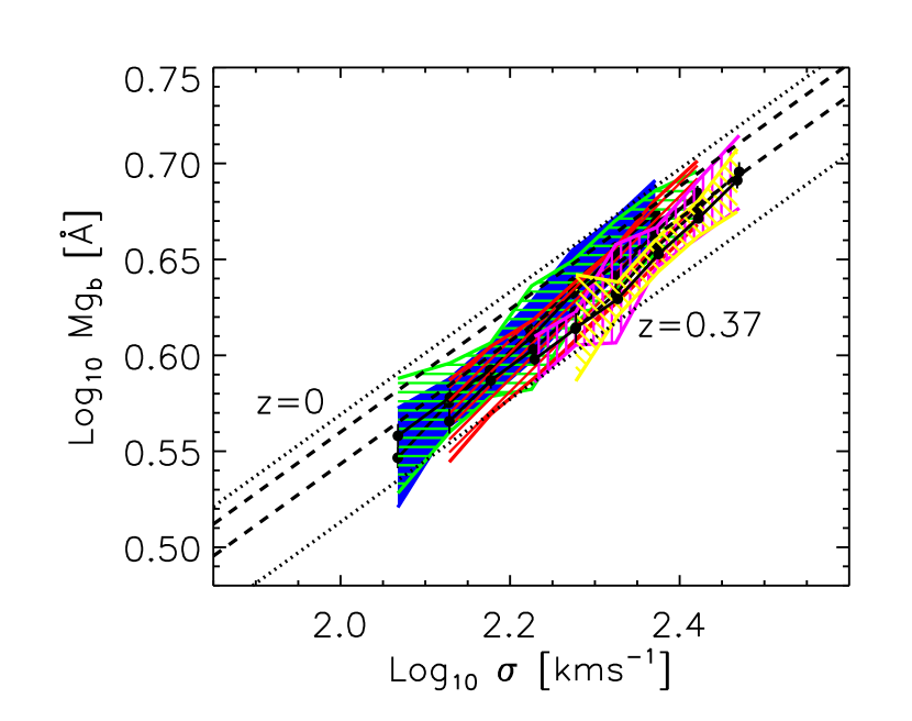
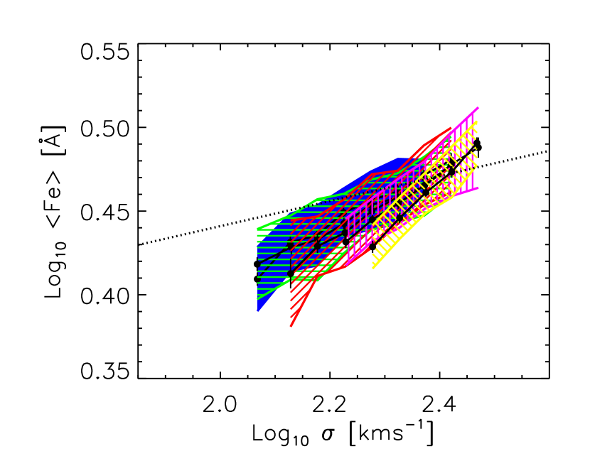
Figure 21: Correlation between the line-index strengths (smoothed to Lick resolution) that are used in Section 6 and velocity dispersion. Top left and right panels show the anti-correlation between H$\beta$ and H$\gamma_{\rm F}$ with $\sigma$. Bottom left and right panels show Mg$b$ and $\langle$Fe$\rangle$ are positively correlated with $\sigma$. Hashed colored regions show these relations in different redshift bins. Dotted lines for H$\beta$ and $\langle{\rm Fe}\rangle$ show the correlations from Jørgenson (1997). For the Mg$b$-$\sigma$ relation, dotted lines show the relation at $z=0$ and $z=0.37$ reported by Bender et al. (1996). Dashed lines show their results interpolated to $z=0.06$ and $z=0.17$ to simplify comparison with our results. The apparent rapid differential evolution of the Fe-$\sigma$ relation is a selection effect.

Figure 21 shows our measurements of the correlations between H$\beta$, H$\gamma_{\rm F}$, Mg$b$, and $\langle{\rm Fe}\rangle$ with velocity dispersion. These are the indices we use in our study of single burst stellar population synthesis models (Section 6). Our measurements are in reasonable agreement with previous work, with the exception of Mg$b$. Our Mg$b$ values are offset to smaller values than those of Bender et al. (1996); this offset is not due to the fact that Bender et al. aperture correct both Mg$b$ and $\sigma$ to a fixed physical scale, whereas we correct to $r_{e}/8$. Shifting our values upwards so they agree with the literature makes little qualitative difference to our conclusions about the ages, metallicities and $\alpha$-enhancements in our sample.

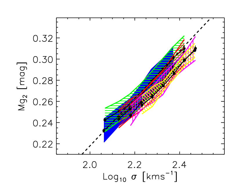
Figure 22: Comparison of correlation between Mg₂ and $\sigma$ reported by Bernardi et al. (1998) (dashed line) and the relation in the present data set (hashed colored regions show the relation in different redshift bins).

As another check, Figure 22 shows that the Mg₂-$\sigma$ correlation and its evolution are consistent with previous work (Bernardi et al. 1998). Using Mg₂ in place of Mg$b$, and making the corresponding change in the SSP models, makes no difference to our findings.

Figure 2: Distribution of the number of galaxies in a composite spectrum (left), and the signal-to-noise ratios of the composites (right). Dashed histogram in left panel shows all composites, and solid histogram shows those with S/N$\geq 40$.

Figure 8: Evolution of observed parameters estimated using early-type galaxies in the entire sample which have $2.35\leq\log_{10}\sigma\leq 2.4$ (dashed, same in all panels), compared to dependence on environment (solid), for galaxies which have the range of redshift and luminosity shown in the top left and top right of each panel, respectively. The time difference between $z\sim 0.17$ and $z\sim 0.06$ is 1.3 Gyr. The top-right panel is different from the others; it happens to contain a supercluster, and this may have compromised our estimates of environment or affected the color. (An asterisk signifies that the quoted rms is for $\log_{10}$ of the index.)

Figure 9: Evolution of observed parameter (dashed/dotted, same in all panels) compared to dependence on environment (solid). Dotted lines correct for flux-calibration problems by dividing measured values by a factor of three (c.f. Appendix B). (An asterisk signifies that the quoted rms is for $\log_{10}$ of the index.) In most cases, the difference between $z\sim 0.17$ and $z\sim 0.06$ is similar to the difference between cluster and less dense environments.

Figure 10: As for the previous figure, but now comparing the evolution of the Lick indices with the dependence on environment. Bottom panel contains a supercluster, so environmental effects may not be accurate. (An asterisk signifies that the quoted rms is for $\log_{10}$ of the index.)

Figure 10: Continued.

Table 1: Composite spectra. Mean values of redshift, evolution-corrected absolute magnitudes, velocity dispersion, effective radius, color, fracDev_r, environment (0 and 1 indicate low and high density environments), as well as the number of galaxies and the mean S/N ratio for the objects which make up each composite are given. This table is available in its entirety in the electronic edition of the Journal.

ID	IDz	$\langle z\rangle$	IDM	$\langle M_{r}\rangle$	$\langle M_{i}\rangle$	IDσ	$\langle{\rm log_{10}}\sigma\rangle$	IDR	$\langle{\rm log_{10}}R\rangle$	$\langle g-r\rangle$	$\langle{\rm fDev}\rangle$	Env	Ng	S/N
				[mag]	[mag]		[km s-1]		[kpc $h^{-1}$]	[mag]
1	1	0.0593	1	$-19.873$	$-20.240$	3	2.131	2	0.119	0.70	0.98	1	3	32
2	1	0.0615	2	$-20.147$	$-20.477$	3	2.120	1	0.058	0.72	0.98	1	3	37
3	1	0.0629	2	$-20.204$	$-20.513$	4	2.178	1	0.075	0.78	0.97	1	2	28
4	1	0.0634	2	$-20.244$	$-20.629$	5	2.228	1	0.047	0.79	0.97	1	5	53
5	1	0.0602	2	$-20.349$	$-20.720$	6	2.266	1	0.028	0.74	1.00	1	2	49

Table 2: Line-strengths and uncertainties measured from the composite spectra given in Table 1. This table is available in its entirety in the electronic edition of the Journal.

ID	OII	err	H$\delta_{A}$	err	H$\delta_{F}$	err	H$\gamma_{A}$	err	H$\gamma_{F}$	err	D4000	err
	[Å]	[Å]	[Å]	[Å]	[Å]	[Å]	[Å]	[Å]	[Å]	[Å]
1	$-1.036$	0.530	$-1.579$	0.420	0.304	0.296	$-4.967$	0.357	$-0.723$	0.231	1.902	0.018
2	$-1.446$	0.484	$-1.996$	0.362	0.362	0.247	$-4.791$	0.291	$-1.260$	0.191	1.865	0.015
3	$-0.210$	0.484	$-1.919$	0.423	0.477	0.286	$-6.164$	0.358	$-1.873$	0.239	1.890	0.017
4	$-1.638$	0.384	$-2.739$	0.265	0.699	0.190	$-5.673$	0.222	$-1.817$	0.142	1.963	0.013
5	0.518	0.352	$-2.508$	0.277	0.120	0.201	$-6.861$	0.243	$-2.527$	0.170	1.956	0.012

Table 3: Lick index-strengths and uncertainties measured from the composite spectra given in Table 1. This table is available in its entirety in the electronic edition of the Journal.

ID	CN1	err	CN2	err	Ca4227	err	G4300	err	Fe4383	err	Ca4455	err	Fe4531	err	C24668	err	H$\beta$	err	Fe5015	err
	[mag]		[mag]		[Å]		[Å]		[Å]		[Å]		[Å]		[Å]		[Å]		[Å]
1	0.092	0.011	0.141	0.011	1.758	0.185	5.974	0.289	6.733	0.306	2.572	0.199	4.561	0.241	6.346	0.309	1.983	0.164	5.959	0.271
2	0.095	0.009	0.123	0.009	1.094	0.161	5.747	0.254	6.022	0.259	2.407	0.166	3.872	0.206	6.102	0.271	2.075	0.144	6.120	0.226
3	0.146	0.012	0.201	0.012	1.347	0.203	6.044	0.305	5.452	0.340	1.756	0.193	4.144	0.277	6.264	0.353	1.326	0.192	6.071	0.298
4	0.120	0.007	0.173	0.007	1.583	0.118	6.248	0.200	5.883	0.199	2.086	0.115	3.723	0.149	7.037	0.189	1.664	0.114	6.181	0.166
5	0.126	0.008	0.171	0.008	1.384	0.117	6.693	0.185	6.066	0.203	2.188	0.118	4.735	0.158	6.668	0.205	1.654	0.109	4.713	0.190

Table 4: Lick index-strengths and uncertainties measured from the composite spectra given in Table 1. This table is available in its entirety in the electronic edition of the Journal.

ID	Mg1	err	Mg2	err	Mg$b$	err	Fe5270	err	Fe5335	err	Fe5406	err	Fe5709	err	Fe5782	err	NaD	err	TiO1	err	TiO2	err
	[mag]		[mag]		[Å]		[Å]		[Å]		[Å]		[Å]		[Å]		[Å]		[mag]		[mag]
1	0.137	0.004	0.256	0.006	3.702	0.186	3.613	0.361	2.543	0.193	2.071	0.156	1.365	0.118	1.367	0.102	3.104	0.140	0.052	0.005	0.095	0.003
2	0.123	0.004	0.253	0.005	4.415	0.158	2.781	0.297	2.871	0.170	2.220	0.137	1.168	0.117	0.774	0.090	3.036	0.124	0.045	0.003	0.082	0.002
3	0.149	0.005	0.284	0.007	4.711	0.209	3.308	0.307	2.340	0.209	1.874	0.186	1.132	0.129	1.182	0.117	3.678	0.175	0.038	0.004	0.086	0.003
4	0.144	0.003	0.287	0.003	4.656	0.108	3.879	0.164	3.115	0.109	2.200	0.094	1.301	0.071	1.015	0.062	3.908	0.092	0.047	0.002	0.090	0.001
5	0.154	0.003	0.291	0.004	4.429	0.128	3.440	0.172	3.512	0.119	2.055	0.106	0.885	0.077	1.024	0.068	3.983	0.093	0.050	0.003	0.092	0.002

Table 5: Dependence of mean and rms residual from the Fundamental Plane on environment, computed using the coefficients of the orthogonal fit, in different bands.

Band	$\langle\Delta\mu\rangle_{\rm high}$	$\langle\Delta\mu\rangle_{\rm low}$	rms$(\Delta\mu)_{\rm high}$	rms$(\Delta\mu)_{\rm low}$
	[mag]	[mag]	[mag]	[mag]
$g$	$0.075\pm 0.006$	$-0.006\pm 0.005$	0.345	0.355
$r$	$0.055\pm 0.006$	$-0.020\pm 0.005$	0.328	0.335
$i$	$0.034\pm 0.006$	$-0.035\pm 0.004$	0.324	0.322

Table 6: Comparison of evolution and environment shown in Figures 8–10. The first column shows the name of the observable; if preceded by the symbol ^∗, then $Y$ in subsequent columns is obtained from $\log_{10}$ of the observable. $\langle Y\rangle$ is the (number weighted) mean of $Y$ over the sample of composites; rms$(Y)$ is the rms spread around this mean. Both the mean and rms are obtained by summing over composite spectra weighting each by the number of galaxies in it. $\Delta Y$(Dens) = $Y$(High Dens)$-Y$(Low Dens). Roman numerals I and II are for galaxies with $-22\leq M_{i}\leq-21$ in redshift bins $0.05<z<0.07$ and $0.07<z<0.09$; Roman numerals III and IV are for galaxies with $-23\leq M_{i}\leq-22$ in redshift bins $0.09<z<0.12$ and $0.12<z<0.14$. The final column shows $\Delta Y$(Evol) $=Y(z\sim 0.06)-Y(z\sim 0.17)$ for galaxies with $2.35\leq\log_{10}\sigma\leq 2.4$; if followed by the superscript ‘¹’, the reported value has been corrected for flux-calibration problems by dividing the observed value by a factor of three (c.f. Appendix B).

Parameter	$\langle Y\rangle$	rms($Y$)	$\Delta Y$(Dens)-I	$\Delta Y$(Dens)-II	$\Delta Y$(Dens)-III	$\Delta Y$(Dens)-IV	$\Delta Y$(Evol)
$M_{r}$ [mag]	-21.91	0.71	$0.054\pm 0.038$	$0.027\pm 0.033$	$0.087\pm 0.035$	$-0.021\pm 0.047$	$0.091\pm 0.028$
${}^{*}\sigma$ [kms-1]	2.26	0.10	$0.001\pm 0.011$	$-0.001\pm 0.010$	$0.002\pm 0.010$	$0.015\pm 0.010$	$0.007\pm 0.009$
${}^{*}R_{o,r}\sigma^{2}$	5.02	0.35	$0.011\pm 0.027$	$0.071\pm 0.023$	$-0.003\pm 0.023$	$0.049\pm 0.026$	$-0.017\pm 0.021$
${}^{*}R_{o,r}$ [kpc $h^{-1}$]	0.49	0.23	$0.004\pm 0.021$	$0.024\pm 0.019$	$0.026\pm 0.020$	$0.006\pm 0.021$	$-0.011\pm 0.017$
$g-r$ [mag]	0.73	0.04	$0.016\pm 0.005$	$0.003\pm 0.004$	$0.024\pm 0.005$	$0.032\pm 0.006$	$0.031\pm 0.004$
fracDev	0.96	0.04	$-0.003\pm 0.006$	$-0.004\pm 0.004$	$-0.002\pm 0.007$	$0.006\pm 0.007$	$0.006\pm 0.004$
OII [Å]	2.29	1.52	$-0.757\pm 0.128$	$-0.759\pm 0.117$	$-0.793\pm 0.151$	$-0.469\pm 0.166$	$-0.702\pm 0.119$
H$\delta_{\rm A}$ [Å]	-1.72	0.93	$-0.358\pm 0.111$	$-0.263\pm 0.080$	$-0.373\pm 0.103$	$-0.421\pm 0.135$	$-0.372\pm 0.073^{1}$
H$\delta_{\rm F}$ [Å]	0.66	0.46	$-0.077\pm 0.062$	$-0.131\pm 0.038$	$-0.057\pm 0.049$	$-0.092\pm 0.066$	$-0.146\pm 0.035^{1}$
H$\gamma_{\rm A}$ [Å]	-5.37	0.85	$-0.287\pm 0.110$	$-0.280\pm 0.082$	$-0.432\pm 0.085$	$-0.399\pm 0.117$	$-0.235\pm 0.064^{1}$
H$\gamma_{\rm F}$ [Å]	-1.41	0.54	$-0.226\pm 0.071$	$-0.138\pm 0.051$	$-0.275\pm 0.051$	$-0.150\pm 0.070$	$-0.118\pm 0.040^{1}$
D4000	1.90	0.08	$0.024\pm 0.009$	$0.026\pm 0.007$	$0.028\pm 0.008$	$0.036\pm 0.010$	$0.035\pm 0.007^{1}$
∗[MgFe]${}^{{}^{\prime}}$	0.58	0.04	$0.021\pm 0.005$	$0.008\pm 0.004$	$0.009\pm 0.004$	$0.017\pm 0.006$	$0.011\pm 0.003$
∗Mg$b$/$\langle$Fe$\rangle$	0.13	0.05	$0.024\pm 0.005$	$0.003\pm 0.004$	$0.003\pm 0.005$	$0.012\pm 0.007$	$0.012\pm 0.003$
CN1 [mag]	0.11	0.03	$0.010\pm 0.004$	$0.002\pm 0.003$	$0.009\pm 0.004$	$0.010\pm 0.004$	$0.010\pm 0.004^{1}$
CN2 [mag]	0.16	0.04	$0.018\pm 0.005$	$-0.002\pm 0.004$	$0.018\pm 0.005$	$0.017\pm 0.006$	$0.010\pm 0.004^{1}$
∗Ca4227 [Å]	0.19	0.06	$0.026\pm 0.007$	$-0.001\pm 0.006$	$0.007\pm 0.007$	$0.019\pm 0.007$	$0.011\pm 0.004^{1}$
∗G4300 [Å]	0.77	0.03	$0.010\pm 0.003$	$0.003\pm 0.003$	$0.008\pm 0.003$	$0.013\pm 0.005$	$0.006\pm 0.002^{1}$
∗Fe4383 [Å]	0.76	0.05	$0.017\pm 0.005$	$0.009\pm 0.005$	$-0.014\pm 0.005$	$0.009\pm 0.007$	$0.010\pm 0.003$
∗Ca4455 [Å]	0.33	0.07	$0.021\pm 0.007$	$0.020\pm 0.006$	$-0.001\pm 0.008$	$0.005\pm 0.010$	$0.005\pm 0.005$
∗Fe4531 [Å]	0.61	0.04	$-0.002\pm 0.004$	$-0.001\pm 0.004$	$-0.003\pm 0.004$	$-0.006\pm 0.005$	$0.004\pm 0.002$
∗C24668 [Å]	0.85	0.06	$-0.003\pm 0.007$	$-0.002\pm 0.006$	$0.021\pm 0.007$	$0.006\pm 0.008$	$0.036\pm 0.005$
∗H$\beta$ [Å]	0.25	0.07	$-0.005\pm 0.008$	$0.002\pm 0.007$	$-0.010\pm 0.008$	$-0.010\pm 0.009$	$-0.013\pm 0.005$
∗Fe5015 [Å]	0.77	0.05	$0.007\pm 0.005$	$0.009\pm 0.004$	$0.020\pm 0.006$	$0.014\pm 0.007$	$-0.002\pm 0.003$
Mg1 [mag]	0.14	0.02	$0.009\pm 0.003$	$0.004\pm 0.002$	$0.006\pm 0.002$	$0.011\pm 0.002$	$0.010\pm 0.002$
Mg2 [mag]	0.27	0.03	$0.015\pm 0.004$	$0.007\pm 0.003$	$0.014\pm 0.004$	$0.011\pm 0.004$	$0.017\pm 0.003$
∗Mg$b$ [Å]	0.64	0.06	$0.026\pm 0.007$	$0.020\pm 0.006$	$0.026\pm 0.006$	$0.016\pm 0.009$	$0.023\pm 0.005$
∗Fe5270 [Å]	0.52	0.05	$0.003\pm 0.005$	$0.005\pm 0.004$	$-0.004\pm 0.005$	$0.009\pm 0.007$	$0.005\pm 0.003$
∗Fe5335 [Å]	0.50	0.06	$0.005\pm 0.006$	$0.004\pm 0.006$	$0.007\pm 0.007$	$0.020\pm 0.008$	$0.004\pm 0.003$
∗Fe5406 [Å]	0.31	0.06	$0.006\pm 0.006$	$0.009\pm 0.005$	$-0.004\pm 0.006$	$0.001\pm 0.009$	$0.005\pm 0.003$
∗Fe5709 [Å]	0.03	0.07	$0.000\pm 0.006$	$0.001\pm 0.007$	$-0.011\pm 0.009$	$-0.018\pm 0.009$	$-0.015\pm 0.004$
∗Fe5782 [Å]	-0.02	0.09	$0.019\pm 0.009$	$0.008\pm 0.008$	$-0.023\pm 0.009$	$-0.011\pm 0.016$	$0.012\pm 0.005$
∗NaD [Å]	0.60	0.08	$0.009\pm 0.009$	$0.002\pm 0.008$	$-0.005\pm 0.008$	$0.026\pm 0.009$	$0.049\pm 0.007$
TiO1 [mag]	0.04	0.01	$0.003\pm 0.001$	$-0.003\pm 0.001$	$0.001\pm 0.001$	$0.003\pm 0.001$	$0.002\pm 0.001$
TiO2 [mag]	0.08	0.01	$0.002\pm 0.001$	$0.004\pm 0.001$	$0.002\pm 0.001$	$0.002\pm 0.001$	$0.004\pm 0.001$

Table 7: Lick index-strengths and uncertainties used to measure age, [Z/H] and [$\alpha$/Fe] from SSP models. These were measured from the composite spectra given in Table 1 after convolving to Lick resolution. This table is available in its entirety in the electronic edition of the Journal.

ID	H$\gamma_{F}$	err	H$\beta$	err	Mg$b$	err	Fe5270	err	Fe5335	err
	[Å]	[Å]	[Å]	[Å]	[Å]	[Å]	[Å]	[Å]	[Å]	[Å]
1	-0.650	0.232	1.887	0.164	3.524	0.187	3.086	0.363	2.018	0.195
2	-0.983	0.192	1.935	0.144	4.138	0.160	2.511	0.298	2.226	0.172
3	-1.664	0.239	1.346	0.191	4.436	0.211	2.843	0.309	1.883	0.211
4	-1.524	0.143	1.654	0.114	4.457	0.108	3.474	0.165	2.531	0.110
5	-2.248	0.170	1.643	0.109	4.370	0.129	2.966	0.173	2.839	0.121

Table 8: Age, [Z/H] and [$\alpha$/Fe] obtained using the Lick index-strengths reported in Table 7 and the SSP models of TMB03-TMK04. Two sets of quantities are reported: the first set of columns were obtained using H$\beta$, Mg$b$ and $\langle{\rm Fe}\rangle$, while the final six columns were obtained after substituting H$\gamma_{\rm F}$ for H$\beta$. Objects with ages set to zero are those for which the models did not return reliable estimates of age, [Z/H] and [$\alpha$/Fe]. This can be either because they lie beyond the model grids, or because the three ways of estimating the ages gave very different answers. This table is available in its entirety in the electronic edition of the Journal.

ID	AgeHβ	err	[Z/H]Hβ	err	[$\alpha/$Fe]Hβ	err	Age${}_{{\rm H}\gamma_{\rm F}}$	err	[Z/H]${}_{{\rm H}\gamma_{\rm F}}$	err	[$\alpha/$Fe]${}_{{\rm H}\gamma_{\rm F}}$	err
	[Gyrs]	[Gyrs]					[Gyrs]	[Gyrs]
1	6.9	2.7	-0.017	0.089	0.102	0.065	4.8	2.4	0.059	0.082	0.123	0.044
2	5.9	2.1	0.105	0.082	0.326	0.059	7.6	3.4	0.062	0.076	0.313	0.042
3	0.0	0.0	0.000	0.000	0.000	0.000	0.0	0.0	0.000	0.000	0.000	0.000
4	8.7	3.3	0.302	0.131	0.144	0.042	6.4	2.4	0.359	0.051	0.162	0.036
5	9.6	3.4	0.225	0.107	0.150	0.069	0.0	0.0	0.000	0.000	0.000	0.000

Table 9: Correlations of derived parameters, age, [Z/H] and [$\alpha$/Fe] with velocity dispersion. The first two rows show the fits (slope and zero-point) to the high density sample at $z=0.06$. The following three rows show the offsets with respect to these fits for these relations at different redshifts. The last four rows show the offsets between different environments at different redshifts; the slope of the fit was kept fixed to the value given by the high density sample at $z=0.06$.

Using H$\beta$	Log10 Age - Log${}_{10}\sigma$	[Z/H] - Log${}_{10}\sigma$	[$\alpha$/Fe] - Log${}_{10}\sigma$
slope	1.15	0.38	0.32
ZP	$-1.72\pm 0.31$	$-0.64\pm 0.013$	$-0.54\pm 0.005$
$\Delta$ZPEvol(z∼0.06-z∼0.08)	$0.27\pm 0.17$ [Gyrs]	$0.008\pm 0.009$	$0.001\pm 0.004$
$\Delta$ZPEvol(z∼0.06-z∼0.11)	$1.21\pm 0.31$ [Gyrs]	$-0.011\pm 0.013$	$-0.002\pm 0.006$
$\Delta$ZPEvol(z∼0.06-z∼0.13)	$0.81\pm 0.47$ [Gyrs]	$0.008\pm 0.019$	$0.005\pm 0.010$
$\Delta$ZPEnv(z∼0.06)	$0.42\pm 0.38$ [Gyrs]	$0.018\pm 0.016$	$0.023\pm 0.006$
$\Delta$ZPEnv(z∼0.08)	$0.41\pm 0.28$ [Gyrs]	$0.016\pm 0.014$	$0.017\pm 0.005$
$\Delta$ZPEnv(z∼0.11)	$-0.27\pm 0.37$ [Gyrs]	$0.044\pm 0.016$	$0.025\pm 0.007$
$\Delta$ZPEnv(z∼0.13)	$0.63\pm 0.55$ [Gyrs]	$0.025\pm 0.022$	$0.017\pm 0.011$
Using H$\gamma_{\rm F}$	Log10 Age - Log${}_{10}\sigma$	[Z/H] - Log${}_{10}\sigma$	[$\alpha$/Fe] - Log${}_{10}\sigma$
slope	0.81	0.58	0.39
ZP	$-0.98\pm 0.23$	$-1.07\pm 0.010$	$-0.68\pm 0.005$
$\Delta$ZPEvol(z∼0.06-z∼0.08)	$0.17\pm 0.14$ [Gyrs]	$0.006\pm 0.007$	$0.002\pm 0.003$
$\Delta$ZPEvol(z∼0.06-z∼0.11)	$0.95\pm 0.20$ [Gyrs]	$-0.003\pm 0.011$	$0.005\pm 0.006$
$\Delta$ZPEvol(z∼0.06-z∼0.13)	$1.17\pm 0.41$ [Gyrs]	$0.001\pm 0.017$	$0.006\pm 0.010$
$\Delta$ZPEnv(z∼0.06)	$0.58\pm 0.28$ [Gyrs]	$0.008\pm 0.013$	$0.022\pm 0.006$
$\Delta$ZPEnv(z∼0.08)	$0.47\pm 0.21$ [Gyrs]	$0.016\pm 0.011$	$0.017\pm 0.005$
$\Delta$ZPEnv(z∼0.11)	$0.60\pm 0.24$ [Gyrs]	$0.015\pm 0.013$	$0.014\pm 0.007$
$\Delta$ZPEnv(z∼0.13)	$0.95\pm 0.46$ [Gyrs]	$0.010\pm 0.020$	$0.014\pm 0.011$

References

- (1) Abazajian, K., et al. 2003, AJ, 126, 2081
- (2) Balogh, M. L., Morris, S. L., Yee, H. K. C., Carlberg, R. G., Ellingson, E. 1999, ApJ, 527, 54
- (3) Balogh, M. L., Christlein, D., Zabludoff, A. I., & Zaritsky, D. 2001, ApJ, 557, 117
- (4) Balogh, M., Eke, V., Miller, C. et al. 2004, MNRAS, 348, 1355
- (5) Bekki, K., Couch, W. J., & Shioya, Y. 2001, PASJ, 53, 395
- (6) Bernardi, M., Renzini, A., da Costa, L. N., Wegner, G., Alonso, M. V., Pellegrini, P. S., Rité, C. & Willmer, C. N. A. 1998, ApJL, 508, 143
- (7) Bernardi, M., Sheth, R. K., Annis, J. et al. 2003a, AJ, 125, 1817
- (8) Bernardi, M., Sheth, R. K., Annis, J. et al. 2003b, AJ, 125, 1849
- (9) Bernardi, M., Sheth, R. K., Annis, J. et al. 2003c, AJ, 125, 1866
- (10) Bernardi, M., Sheth, R. K., Annis, J. et al. 2003d, AJ, 125, 1882
- (11) Bernardi, M., Sheth, R. K., Nichol, R. C. et al. 2005, AJ, 129, 61
- (12) Blanton, M.R., Lupton, R.H., Maley, F.M., Young, N., Zehavi, I., & Loveday, J. 2003, AJ, 125, 2276
- (13) Bower, R. G., Lucey, J. R., & Ellis, R. S. 1992a, MNRAS, 254, 589
- (14) Bower, R. G., Lucey, J. R., & Ellis, R. S. 1992b, MNRAS, 254, 601
- (15) Bruzual, G., & Charlot, S. 2003, MNRAS, 344, 1000
- (16) Carretero, C., Vazdekis, A., Beckman, J. E., Sanchez-Blazquez, P., & Gorgas, J. 2004, ApJL, 609, 45
- (17) Colless, M., Burstein, D., Davies, R. L., McMahan, R. K., Saglia, R. P., & Wegner, G. 1999, MNRAS, 303, 813
- (18) Djorgovski, S. & Davis, M. 1987, ApJ, 313, 59
- (19) Dressler, A., Lynden-Bell, D., Burstein, D., Davies, R. L., Faber, S. M., Terlevich, R. J., & Wegner, G. 1987, ApJ, 312, 42
- (20) Eisenstein, D.J., Annis, J., Gunn, J.E., et al. 2001, AJ, 122, 2267
- (21) Eisenstein, D. J. 2003, ApJ, 586, 718
- (22) Faber, S. M., & Jackson, R. 1976, ApJ, 204, 668
- (23) Fukugita, M., Ichikawa, T., Gunn, J.E., Doi, M., Shimasaku, K., & Schneider, D.P. 1996, AJ, 111, 1748
- (24) Gunn, J. E., & Gott, J. R. III 1972, ApJ, 176, 1
- (25) Gunn, J.E., Carr, M.A., Rockosi, C.M., Sekiguchi, M., et al. 1998, AJ, 116, 3040
- (26) Hogg, D.W., Schlegel, D.J., Finkbeiner, D.P., & Gunn, J.E. 2001, AJ, 122, 2129
- (27) Hogg, D. W.;, Blanton, M. R., Brinchmann, J. et al. 2004, ApJL, 601, 29
- (28) Jørgensen, I. 1997, MNRAS, 288, 161
- (29) Kauffmann, G. 1996, MNRAS, 281, 487
- (30) Kauffmann, G. & Charlot, S. 1998, MNRAS, 294, 705
- (31) Kauffmann, G., Heckman, T. M., Tremonti, C. et al. 2003, MNRAS, 346, 1055
- (32) Kelson, D. D., Illingworth, G. D., Franx, M., van Dokkum, P. G. 2001, ApJL, 552, 17
- (33) Kodama, T., Arimoto, N., Barger, A. J., & Arag’on-Salamanca, A. 1998, A&A, 334, 99
- (34) Kuntschner, H., Lucey, J. R., Smith, R. J., Hudson, M. J., & Davies, R. L. 2001, MNRAS, 323, 615
- (35) Kuntschner, H. 2004, A&A, in press (astro-ph/0407219)
- (36) Lacey, Cedric, & Cole, Shaun 1993, MNRAS, 262, 627
- (37) Lupton, R., Gunn, J. E., Ivezić, Z., Knapp, G. R., Kent, S., & Yasuda, N. 2001, in ASP Conf. Ser. 238, Astronomical Data Analysis Software and Systems X, ed. F. R. Harnden, Jr., F. A. Primini, and H. E. Payne (San Francisco: Astr. Soc. Pac.), p. 269 (astro-ph/0101420)
- (38) Miller, C. J., Nichol, R. C., Reichart, D. et al. 2004, AJ, submitted
- (39) Mo, H. J., & White, S. D. M. 1996, MNRAS, 282, 347
- (40) Moore, B., Lake, G., Quinn, T., & Stadel, J. 1999, MNRAS, 304, 465
- (41) Nelan J. E., Smith R. J., Hudson M. J., Wegner G. A., Lucey J. R., Moore S. A. W., Quinney S. J., Suntzeff N. B., ApJ, in press (astro-ph/0505301)
- (42) Petrosian, 1976, ApJ, 209, L1
- (43) Pier, J.R., Munn, J.A., Hindsley, R.B., Hennessy, G.S., Kent, S.M., Lupton, R.H., & Ivezic, Z. 2003, AJ, 125, 1559
- (44) Poveda, A. 1961, ApJ, 134, 910
- (45) Sandage, A., & Visvanathan, N., 1978a, ApJ, 223, 707
- (46) Sandage, A., & Visvanathan, N., 1978b, ApJ, 225, 742
- (47) Smith, J.A., Tucker, D.L., Kent, S.M., et al. 2002, AJ, 123, 2121
- (48) Stoughton, C., Lupton, R.H., Bernardi, M., et al. 2002, AJ, 123, 485
- (49) Strauss, M.A., Weinberg, D.H., Lupton, R.H. et al. 2002, AJ, 124, 1810
- (50) Tantalo, R., Chiosi, C., & Bressan, A. 1998, A& A, 333, 490
- (51) Tantalo, R. & Chiosi, C. 2004, MNRAS, 353, 917
- (52) Thomas, D., Maraston, C., & Bender, R. 2003, MNRAS, 339,897 (TMB03)
- (53) Thomas D., Maraston C., Korn, A., 2004, MNRAS, 352, L19 (TMK04)
- (54) Thomas, D., Maraston, C., Bender, R., & de Oliveira, C. M. 2005, ApJ, 621, 673
- (55) Trager, S. C., Worthey, G., Faber, S. M., Burstein, D., & González, J. J. 1998, ApJS, 116, 1
- (56) Vazdekis, A., Casuso, E., Peletier, R. F., & Beckman, J. E. 1996, ApJS, 106, 307
- (57) Wake, D. A., Collins, C. A., Nichol, R. C., Jones, L. R., Burke, D. J. 2005, ApJ, 627, 186
- (58) White, S. D. M., & Rees, M. J. 1978, MNRAS, 183, 341
- (59) White, S. D. M. & Frenk, C. 1991, ApJ, 379, 52
- (60) Worthey, G. 1994, ApJS, 95, 107
- (61) Worthey, G., Faber, S. M., Gonzalez, J. J., & Burstein, D. 1994, ApJS, 94, 687
- (62) Worthey, G. & Ottaviani, D. L. 1997, ApJS, 111, 377
- (63) York, D.G., Adelman, J., Anderson, J.E., et al. 2000, AJ, 120, 1579