Turbulent Angular Momentum Transport
in Weakly-Ionized Accretion Disks

Abstract

Accretion disks are ubiquitous in the universe. Although difficult to observe directly, their presence is often inferred from the unique signature they imprint on the spectra of the systems in which they are observed. In addition, many properties of accretion-disk systems that would be otherwise mysterious are easily accounted for by the presence of matter accreting (accumulating) onto a central object. Since the angular momentum of the infalling material is conserved, a disk naturally forms as a repository of angular momentum. Dissipation removes energy and angular momentum from the system and allows the disk to accrete. It is the energy lost in this process and ultimately converted to radiation that we observe.

Understanding the mechanism that drives accretion has been the primary challenge in accretion disk theory. Turbulence provides a natural means of dissipation and the removal of angular momentum, but firmly establishing its presence in disks proved for many years to be difficult. The realization in the 1990s that a weak magnetic field will destabilize a disk and result in a vigorous turbulent transport of angular momentum has revolutionized the field. Much of accretion disk research now focuses on understanding the implications of this mechanism for astrophysical observations. At the same time, the success of this mechanism depends upon a sufficient ionization level in the disk for the flow to be well-coupled to the magnetic field. Many disks, such as disks around young stars and disks in binary systems that are in quiescence, are too cold to be sufficiently ionized, and so efforts to establish the presence of turbulence in these disks continues.

This dissertation focuses on several possible mechanisms for the turbulent transport of angular momentum in weakly-ionized accretion disks: gravitational instability, radial convection and vortices driving compressive motions. It appears that none of these mechanisms are very robust in driving accretion. A discussion is given, based on these results, as to the most promising directions to take in the search for a turbulent transport mechanism that does not require magnetic fields. Also discussed are the implications of assuming that no turbulent transport mechanism exists for weakly-ionized disks.

“Since we astronomers are priests of the highest God in regard to the book of nature, it benefits us to be thoughtful, not of the glory of our minds, but rather, above all else, of the glory of God.”

– Johannes Kepler

Soli Deo gloria

List of Figures

List of Figures

1. 1.1 Schematic of a cataclysmic variable system.
2. 1.2 Mechanical analogy for the MRI.
3. 1.3 Local coordinate system at $t=0$.
4. 2.1 Evolution of the kinetic, gravitational, and thermal energy per unit area in the standard run.
5. 2.2 Evolution of the gravitational and hydrodynamic pieces of ${\langle}\alpha{\rangle}$ in the standard run.
6. 2.3 Map of surface density in the standard run.
7. 2.5.2 Varying $\Sigma_{o}$ and $\Omega$
8. 2.5.2 Varying $\Sigma_{o}$ and $\Omega$
9. 2.8 Mean gravitational potential energy as a function of initial cooling time for a series of models with varying initial cooling time and $T_{o}=1200$.
10. 2.9 Initial cooling times at the points of non-fragmentation, fragmentation and transition.
11. 2.5.2 Varying $\Sigma_{o}$ and $\Omega$
12. 2.12 Time-averaged shear stress vs. effective cooling time for a series of runs.
13. 3.1 A summary of analytic results for shwaves (shearing waves) in a stratified disk.
14. 4.5 Numerical Model
15. 4.3 Evolution of $v_{t}$ as a function of time for Run 2 (external potential, non-rotating frame).
16. 4.6.1 External Potential in Non-Rotating Frame
17. 4.6 Snapshots of the entropy in the nonlinear regime for Run 2.
18. 4.7 Evolution of $v_{t}$ as a function of time for Run 3 (external potential, rotating frame).
19. 4.8 Snapshots of the entropy in the nonlinear regime for Run 3.
20. 4.9 Evolution of $v_{t}$ as a function of time for Run 4 ($q=0$, rotating frame).
21. 4.10 Snapshots of the entropy in the nonlinear regime for Run 4.
22. 4.11 Evolution of the dimensionless angular momentum flux due to radial convection.
23. 4.12 Growth rates as a function of azimuthal boost.
24. 4.13 Growth rates as a function of $q$.
25. 4.14 Evolution of $v_{t}$ as a function of time for Run 7.
26. 4.15 Evolution of the density perturbation for Run 8.
27. 4.16 Parameter space surveyed in a search for nonlinear instabilities.
28. 4.17 Evolution of $v_{t}$ as a function of time for Run 10.
29. 5.3.2 Code Verification
30. 5.3 Evolution of the potential vorticity in the fiducial run.
31. 5.4 Results
32. 5.6 Evolution of kinetic energy in time for the fiducial run.
33. 5.7 Evolution of the shear stress $\alpha$ in the fiducial run and a set of runs at lower resolutions.
34. 5.4 Results
35. 5.4 Results
36. 5.4 Results
37. 6.1 Ionization structure of YSO disks.

List of Tables

List of Tables

1. 1.1 Example Accretion-Disk Systems
2. 2.1 Scaling Exponent for Cooling Time as a Function of Surface Density
3. 4.1 Summary of Code Runs

Chapter 1 Introduction

Accretion disks form around gravitating objects because the angular momentum of the infalling gas is conserved. In order for the gas to accrete, however, its angular momentum must be removed. Understanding the mechanism underlying this angular momentum transport is a long outstanding puzzle in accretion disk theory. Much progress has been made in recent decades through the realization that a weak magnetic field will destabilize the flow in an ionized disk and result in a turbulent transport of angular momentum. One of the key features of this mechanism, however, is that the gas in the disk must be sufficiently ionized to couple to the magnetic field. It is likely that there are portions of disks, and perhaps entire classes of disks, in which the ionization is too low for the gas to destabilize. The search for a turbulent transport mechanism in weakly-ionized disks continues, therefore, to this day, in an effort to place our understanding of the evolution of these disks on as firm a theoretical footing as that for ionized disks. My research, in collaboration with Charles Gammie, has focused on several possible mechanisms: self-gravity, radial convection and vortices driving compressive disturbances. This dissertation summarizes our main results and discusses their relevance to the question of what drives accretion in weakly-ionized disks.

The purpose of this chapter is to describe all of these ideas in detail and put them in their astrophysical context. I begin in §1.1 with an overview of accretion disks: the systems in which they are observed and their general properties. The importance of angular momentum transport for the evolution of disks is discussed in §1.2, followed by a more detailed discussion of angular momentum transport in both ionized and weakly-ionized disks (§§1.3 and 1.4). I give a brief overview in §1.5 of the model that is used throughout the dissertation for analytic and numerical studies. §1.6 looks ahead to Chapter 6 in which I summarize and chart a course for future work.

1.1 Accretion Disks

An accretion disk is a roughly cylindrical distribution of matter in orbit around a gravitating central object. It is supported against the gravitational pull of its host object primarily by the centrifugal forces arising from the angular momentum of the orbiting material. This support is slightly compromised, however, by the presence of dissipation or the application of external torques. As a result, angular momentum is redistributed through the disk and some of the disk material falls onto the central object, i.e., it accretes. The gravitational potential energy lost during this process is typically converted into radiation, which is the basis for our observations of accretion disk systems. Although disks are rarely observed directly (i.e., by being resolved in a telescope image), they imprint a unique signature on the spectra of their host systems. In addition, the accretion-disk paradigm easily accounts for many properties of astrophysical systems that would be difficult to explain otherwise.

The material in an accretion disk covers a wide range of density and temperature scales [Balbus and Hawley, 1998]. In most cases, collisional mean free paths are extremely short compared to the length scales of interest, and mean times between collisions are short compared to the time scales of interest. Disks are therefore usually modeled as a continuous fluid, using the macroscopic equations of gas dynamics rather than the microscopic equations of kinetic theory. If the fluid is ionized, it is referred to as a plasma.

Accretion disks are found in a variety of astrophysical settings, including compact binary systems (with a white dwarf, black hole, or neutron star), active galactic nuclei (AGN), and young stars. AGN consist of a supermassive black hole ($M\sim 10^{8}{M_{\odot}}$) surrounded by an accretion flow. The presence of a disk in AGN is inferred primarily from the large luminosities of these systems, luminosities that cannot be accounted for by stellar nuclear burning but are easily provided by the large gravitational energy of the compact object. A spectacular exception to this indirect verification is the system NGC4258, an AGN in which the disk is directly observed via maser emission [Watson and Wallin, 1994]. Low Mass and High Mass X-Ray Binary (LMXRB and HMXRB) systems consist of a neutron star (NS) or black hole (BH) accreting matter from its companion; Cataclysmic Variables (CV) are binary systems in which the accreting object is a white dwarf (see Figure 1.1). The variability observed in these systems can be accounted for by models in which instabilities in a disk surrounding the compact object give rise to episodic accretion. Young Stellar Objects (YSO) are pre-main-sequence stars with a circumstellar disk, also known as protoplanetary disks since they are thought to be the sites of planet formation. The presence of a disk in these systems is confirmed in many cases by direct observation (e.g., Burrows et al. 1996).

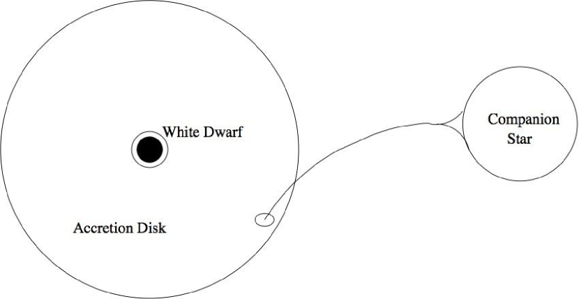
Figure 1.1: Schematic of a cataclysmic variable system.

Table 1.1: Example Accretion-Disk Systems

System	Type	$\frac{M}{{M_{\odot}}}$	$\frac{\dot{M}}{{M_{\odot}}{\rm\,yr}^{-1}}$	$\frac{L_{acc}}{{L_{\odot}}}$	$R_{c}$ (cm)	$T$ (K)	$\frac{H}{R_{c}}$
NGC 4258	AGN	$4\times 10^{7}$	$1\times 10^{-2}$	$1\times 10^{10}$	$1\times 10^{18}$	$7\times 10^{2}$	$2\times 10^{-3}$
Sco X-1	LMXRB-NS	$1$	$1\times 10^{-8}$	$3\times 10^{4}$	$1\times 10^{10}$	$3\times 10^{5}$	$5\times 10^{-2}$
LMC X-3	HMXRB-BH	$10$	$1\times 10^{-8}$	$1\times 10^{4}$	$1\times 10^{11}$	$7\times 10^{4}$	$3\times 10^{-2}$
UX Uma	CV	$0.5$	$1\times 10^{-8}$	$1\times 10^{1}$	$1\times 10^{10}$	$2\times 10^{5}$	$6\times 10^{-2}$
TW Hydrae	YSO	$0.7$	$5\times 10^{-10}$	$1\times 10^{-2}$	$1\times 10^{13}$	$1\times 10^{2}$	$2\times 10^{-2}$

Table 1.1 lists typical values for various physical properties of these systems. The mass of the accreting object is denoted by $M$ in Table 1.1, in units of the solar mass (${M_{\odot}}=2.0\times 10^{33}$ g), and the accretion rate by $\dot{M}$. The accretion luminosity

$$L_{acc}\equiv\frac{GM\dot{M}}{R_{in}}$$ (1.1)

(where $R_{in}$ is the inner radius of the disk and where $G=6.673\times 10^{-8}{\rm\,cm}^{3}{\rm\,g}^{-1}{\rm\,s}^{-2}$ is the gravitation constant) is given in units of the solar luminosity (${L_{\odot}}=3.9\times 10^{33}{\rm\,erg}{\rm\,s}^{-1}$). $R_{c}$ is a characteristic radius for the accretion disk, and $T$ is a characteristic temperature. The final column in Table 1.1 contains the ratio of the vertical scale height $H$ to the local radius. Here

$$H\equiv\frac{c_{s}}{\Omega_{K}},$$ (1.2)

where $c_{s}$ is the isothermal sound speed and

$$\Omega_{K}=\sqrt{\frac{GM}{r^{3}}}$$ (1.3)

is the local Keplerian orbital frequency. The values for $T$ and $H$ in Table 1.1 are obtained from the standard $\alpha$-disk model, a derivation of which is outlined in the following section, using $\alpha=0.01$. Values for the other quantities in Table 1.1 were obtained from the literature (NGC4258: Miyoshi et al. 1995, Gammie et al. 1999; Sco X-1: Vrtilek et al. 1991; LMC X-3: Paczyński 1983, van Paradijs 1996; UX Uma: Frank et al. 1981; TW Hydrae: Muzerolle et al. 2000, Wilner et al. 2003). The standard disk model assumes that the internal energy of the disk material is efficiently radiated from the surfaces of the disk. One implication of this assumption is that the disk is typically quite thin, as can be seen from the last column of Table 1.1. In addition, if the mass of the disk is much less than the mass of the central star, the orbital frequency of the gas $\Omega=\Omega_{K}+O(H/r)^{2}$, so thin, low-mass disks have a nearly-Keplerian rotation profile.

1.2 Angular Momentum Transport and Disk Evolution

The accretion process consists of a net inward transport of matter and a net outward transport of angular momentum; a small fraction of the matter carries angular momentum outward, enabling the bulk of the matter to accrete. This angular momentum transport can take place 1) internally via a local exchange of momentum between fluid elements at adjacent radii or 2) externally via a global mechanism such as the removal of angular momentum by a wind off the surface of the disk (e.g. Blandford and Payne 1982). The focus of this dissertation is on the former: the internal diffusion of angular momentum. While global mechanisms such as winds and jets are certain to play a role in many accretion systems, their operation likely depends in a complicated manner upon the details of each particular system. Standard disk modeling typically ignores their effects and assumes that angular momentum is transported internally (e.g., Pringle 1981, Ruden and Pollack 1991, Sterzik and Morfill 1994, Narita et al. 1994, Stepinski 1997, Gammie 1999). Whether or not it is possible to isolate this aspect of disk evolution and get meaningful results is a question that can only be answered as more comprehensive disk models are developed.

As an example of the importance of global effects, as well as some of the difficulties involved in modeling them, consider the torques from MHD winds (axisymmetric pressure-driven winds have zero torque). Outflows are widely observed from YSO, and it is likely that the outflows are magnetically driven. Outflows are more common in young, high-accretion-rate systems. Highly uncertain estimates for the mass loss rate suggest that about $10\%$ of the accreted mass goes into the jet and associated outflow. What is even less certain is the amount of angular momentum in the outflows, and therefore the role that they play in the evolution of disks on large scales (as opposed to the disk at radii less than a few tenths of an AU). Wind models exist (e.g., Blandford and Payne 1982, Shu et al. 1994, 2000, Wardle and Königl 1993), but there are large gaps in our understanding. We do not know what the strength of the mean vertical magnetic field, which organizes the wind, ought to be, nor how that mean field is transported radially through the disk, nor how the wind evolves in time. A nice summary of this situation is given in Königl and Pudritz [2000].

Molecular shear viscosity is a natural mechanism for coupling fluid elements locally and transporting angular momentum internally, but the large Reynolds numbers of astrophysical flows (due to the large length scales involved) imply molecular shear viscosities that are much too tiny to account for the observations. The coupling due to molecular viscosity is simply too weak to explain the rapid variability and accretion rates that are observed. For example, the outburst duration in CV ranges from $2-20$ days, with the interval between outbursts ranging from tens of days to tens of years [Warner, 1995]. The timescale for viscous diffusion over a distance $l$ due to molecular viscosity is $l^{2}/\nu_{m}$, where $\nu_{m}$ is the molecular (or kinematic) shear viscosity. Using a value $\nu_{m}=10^{5}{\rm\,cm}{\rm\,s}^{-1}$ and a characteristic distance $l=10^{10}{\rm\,cm}$ (see Balbus 2003 and Table 1.1) yields a viscous timescale of about $10^{7}$ years, which is orders of magnitude too large to account for the timescales of CV outbursts.

Standard disk modeling circumvents this problem by assuming the presence of an enhanced “anomalous viscosity” due to turbulence. The large Reynolds numbers are used to advantage, since our experience with laboratory flows indicates that the onset of turbulence typically occurs above a critical Reynolds number. The assumption of turbulent flow, along with the picture of turbulent eddies exchanging momentum with one another to drive accretion, underlies the majority of the phenomenological disk modeling that is currently used to explain observations.

The construction of a standard model for disk evolution proceeds as follows. We will use a cylindrical coordinate system centered on the accreting object, with $r$, $\phi$ and $z$ the radial, azimuthal and vertical coordinates, respectively. We start with mass conservation:

$$\frac{\partial\rho}{\partial t}=-\frac{1}{r}\partial_{r}(r\rho v_{r})-\frac{\partial}{\partial z}(\rho v_{z})$$ (1.4)

where $\rho$ is the mass density and we assume axisymmetry ($\partial/\partial\phi=0$), on average. Integrating this equation vertically through the disk gives

$$\frac{\partial\Sigma}{\partial t}=-\frac{1}{r}\partial_{r}(r\Sigma\bar{v}_{r})+\dot{\Sigma}_{ext}$$ (1.5)

where $\Sigma=\int dz\rho$ is the surface density, $\bar{v}_{r}$ is a vertical average of the radial velocity, and $\dot{\Sigma}_{ext}$ is the difference of $-\rho v_{z}$ evaluated at the upper and lower surface of the disk. It includes infall onto the disk, mass loss in winds, and mass loss through photoevaporation. It is positive when mass flows into the disk, and negative when mass flows out.

The problem now is to find the radial velocity $\bar{v}_{r}$, which we can do using angular momentum conservation:

$$\frac{\partial(\rho l)}{\partial t}=-\frac{1}{r}\frac{\partial}{\partial r}(r^{2}\Pi_{r\phi})-\frac{\partial}{\partial z}(r\Pi_{z\phi}).$$ (1.6)

Here $\rho l$ is evidently the local density of angular momentum, and the right hand side of the equation is the divergence of an angular momentum flux density. $\Pi_{r\phi}$ is a component of the stress tensor, sometimes referred to as the shear stress, with dimensions of pressure; it is the flux density of $\phi$ momentum in the $r$ direction. Likewise $\Pi_{z\phi}$ is the flux density of $\phi$ momentum in the $z$ direction. Again integrating vertically,

$$\frac{\partial(\Sigma l)}{\partial t}=-\frac{1}{r}\frac{\partial}{\partial r}(r^{2}W_{r\phi}+r\Sigma\bar{v}_{r}l)+\tau+l\dot{\Sigma}_{ext}.$$ (1.7)

Here

$$W_{r\phi}\equiv\int dz\Pi_{r\phi}-r\Sigma\bar{v}_{r}l$$ (1.8)

is the integrated shear stress, but with one piece of it, proportional to the radial mass flux, peeled off. In models which assume that angular momentum transport is due to turbulence, $W_{r\phi}$ is referred to as the “turbulent shear stress.” The external torque

$$\tau\equiv-r\Pi_{z\phi}|_{\rm lower}^{\rm upper}-l\dot{\Sigma}_{ext}$$ (1.9)

is the angular momentum flux into the upper and lower surface of the disk with one piece, proportional to the mass flux into the disk, peeled off. $\tau$ includes the effects of, e.g., MHD winds; it is positive when angular momentum flows into the disk and negative when angular momentum flows out. In a steady state ($\partial/\partial t=0$), the condition $W_{r\phi}>0$ must be met for an outward transport of angular momentum and inward accretion.

The mass and angular momentum conservation equations (1.5) and (1.7) can be combined into a single equation governing the evolution of thin, Keplerian disks (multiply the continuity equation by $rv_{\phi}$, subtract the angular momentum equation, solve for $\bar{v}_{r}$, substitute back into the continuity equation):

$$\frac{\partial\Sigma}{\partial t}=\frac{2}{r}\frac{\partial}{\partial r}\left(\frac{1}{r\Omega}\frac{\partial}{\partial r}(r^{2}W_{r\phi})\,-\,\frac{\tau}{\Omega}\right)\,+\,\dot{\Sigma}_{ext}.$$ (1.10)

If we assume that the shear stress $W_{r\phi}$ is due to an anomalous viscosity $\nu$, and that the external torques and mass loss/infall are negligible, equation (1.10) becomes the basic equation for standard disk modeling:

$$\frac{\partial\Sigma}{\partial t}=\frac{3}{r}\frac{\partial}{\partial r}\left(\frac{1}{r\Omega}\frac{\partial}{\partial r}(r^{2}\Sigma\nu\Omega)\right).$$ (1.11)

In a steady state one can show that the accretion rate (inward mass flux $=-2\pi\Sigma r\bar{v}_{r}$) is given by

$$\dot{M}=3\pi\Sigma\nu.$$ (1.12)

In addition to setting $\tau$ and $\dot{\Sigma}_{ext}$ to zero, standard disk theory usually sets $\nu=\alpha c_{s}H$, which parameterizes our ignorance of $W_{r\phi}$. If one reasonably assumes that the turbulent stress (an off-diagonal component of the stress tensor) must be associated with a pressure (an isotropic, diagonal component of the stress tensor), then $\alpha\lesssim 1$. Most disk evolution models take $\alpha=const.$, or allow it to assume a few discrete values. For a disk around a solar-type star with a temperature of $300{\rm\,K}$ at $1$ AU, this yields $\dot{M}=9.9\times 10^{-9}\alpha\Sigma{\rm\,M_{\odot}}{\rm\,yr}^{-1}$, or $\sim 10^{-8}{\rm\,M_{\odot}}{\rm\,yr}^{-1}$ for $\alpha=0.01$ and $\Sigma=10^{2}{\rm\,g}{\rm\,cm}^{-2}$, roughly consistent with observed accretion rates [e.g. Gullbring et al., 1998].

1.3 Angular Momentum Transport in Ionized Disks

While phenomenological disk modeling can proceed along its merry way without a clear demonstration of the onset of turbulence in accretion disk flows, recent progress towards a first-principles understanding of disk turbulence has raised the possibility that more physically-motivated disk models can be developed. The primary breakthrough in our understanding came with the realization that the presence of a weak magnetic field destabilizes a disk on a dynamical time scale, resulting in the onset of magnetohydrodynamic (MHD) turbulence and a vigorous outward flux of angular momentum [Balbus and Hawley, 1991, 1998, Balbus, 2003].

This section gives a summary of the essential physics of this instability, generally termed the magneto-rotational instability, or MRI. The importance of ionization for the successful operation of the MRI in driving turbulence is also discussed, which leads in the following section to an overview of the main question addressed by this dissertation: what drives accretion in disks that are too weakly ionized to be unstable to the MRI?

1.3.1 Magneto-Rotational Instability

The MRI grows directly through exchange of angular momentum between radially-separated fluid elements. This can be understood with a simple mechanical analogy introduced by Balbus and Hawley [1992] and illustrated in Figure 1.2.

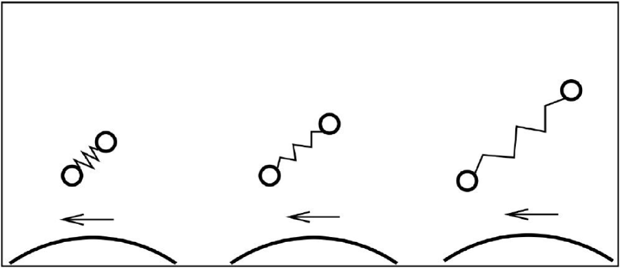
Figure 1.2: Mechanical analogy for the MRI. Two masses, orbiting in the direction indicated by the arrow about a massive body (bottom of the frame), are connected by a spring. The outer mass has higher angular momentum and lower orbital frequency. The lower mass is pulled back in its orbit by the spring, reducing its angular momentum. It sinks to a lower orbit, where it orbits faster, stretching the string and increasing the torque. A runaway ensues. The masses may be thought of as fluid elements connected by a magnetic field.

Imagine that two small masses orbit with frequency $\Omega(r)$ about a third, massive body. The masses are coupled by a spring; the natural frequency of the spring-mass system is $\gamma$. If $\gamma\gg\Omega$, the bodies behave like a perturbed harmonic oscillator. But if $\gamma$ is lowered until $\gamma\sim\Omega$ the orbital motion of the bodies begins to influence the dynamics, and something interesting happens. The outer mass has higher angular momentum but lower orbital frequency. It is pulled forward in its orbit by the spring; its angular momentum increases, moves to a higher orbit, and lowers its orbital frequency further. This stretches the spring, increases the rate at which the outer body gains angular momentum, and a runaway ensues. The outer body heads outward, acquiring angular momentum from the inner body. The inner body moves in a mirror image of the outer body as it loses angular momentum and falls inward.

There is an exact correspondence between the modes of the spring-mass model and the MRI. One can think of the masses as fluid elements and the spring as magnetic field. The field has characteristic frequency $\gamma\sim v_{A}/\lambda$, where $\lambda$ is the separation of the masses and $v_{A}=B/\sqrt{4\pi\rho}$ is the Alfvén speed. $v_{A}/\lambda\lesssim\Omega$ implies instability.

The simplicity of the dynamics shown in Figure 1.2 suggests that the MRI is robust. Instability requires the presence of a weak (subthermal, i.e. $B^{2}/(8\pi\rho)\lesssim c_{s}^{2}$) magnetic field. A stronger magnetic field seems unlikely (it would likely be ejected from the disk by magnetic buoyancy), but if it were present it would likely be associated with other, even more powerful instabilities. The MRI also requires an angular velocity that decreases outward ($d\Omega^{2}/d\ln r<0$), which is always satisfied in Keplerian disks ($\Omega\propto r^{-3/2}$). The maximum growth rate is $\sim\Omega$, independent of the field strength (unless diffusive effects are present). This surprising fact is easily understood once one realizes that the scale $\lambda$ of the instability decreases with the field strength: $\lambda\sim v_{A}/\Omega$.

What does the MRI tell us about $W_{r\phi}$, the key quantity in the evolution equation? Numerical integration of the compressible MHD equations shows that the linear MRI initiates nonlinear turbulence. In the turbulent state one can measure the average value of

$$W_{r\phi}=\int dz\left(\rho v_{r}\delta v_{\phi}-\frac{B_{r}B_{\phi}}{4\pi}\right)$$ (1.13)

where $\delta v_{\phi}$ is the noncircular azimuthal component of the velocity. There are two distinct contributors to the shear stress: hydrodynamic velocity fluctuations, and magnetic field fluctuations, sometimes referred to as the Reynolds and Maxwell stresses. Then $\alpha=const.\times W_{r\phi}/(\Sigma c_{s}^{2})$ (the constant is a matter of convention and takes several values in the literature). Local numerical models yield $\alpha\approx 0.01$ [Hawley et al., 1995, Matsumoto and Tajima, 1995, Hawley et al., 1996, Matsuzaki et al., 1997]. Global numerical models yield similar but slightly larger values [e.g. Armitage, 1998, Hawley, 2000, Machida et al., 2000, Arlt and Rüdiger, 2001].

The presence of turbulence does not guarantee the $W_{r\phi}>0$ necessary for outward angular momentum transport and accretion. For example, the turbulence associated with vertical convection can produce $\alpha<0$ [Stone and Balbus, 1996, Cabot, 1996]. Also, vortices in nearly incompressible disks produce $\alpha\approx 0$ (see Chapter 5). The fact that MRI-driven turbulence has $W_{r\phi}>0$ is thus a nontrivial result, although one that might have been anticipated because of the central role of angular momentum exchange in driving the linear MRI.

1.3.2 MRI in Low-Ionization Disks

MRI-generated MHD turbulence is the likely angular momentum transport mechanism in AGN and in binary systems during outbursts. In portions of YSO disks, however, as well as in CV disks and X-Ray transients in quiescence [Stone et al., 2000, Gammie and Menou, 1998, Menou, 2000], the plasma is cool and nearly neutral. The conductivity of the gas is small by astrophysical standards and the field is no longer frozen into the gas. In some regions the field may be completely decoupled from the fluid, just as the Earth’s lower atmosphere is decoupled from the Earth’s magnetic field.

Low ionization levels change the field evolution through three separate effects: Ohmic diffusion, Hall drift, and ambipolar diffusion. Following the beautiful discussion of Balbus and Terquem [2001] [see also Wardle, 1999, Desch, 2004], a measure of the correction to the field evolution equation (1.21) due to Ohmic diffusion is given by the magnetic Reynolds number $Re_{M}^{-1}\equiv\eta/(v_{A}H)$, where $\eta=c^{2}/(4\pi\sigma_{e})$ is the resistivity, $c$ is the speed of light and the conductivity $\sigma_{e}$ is proportional to the collision timescale for electrons with neutrals. Then

$$Re_{M}\simeq 2\times 10^{19}B\left(\frac{r}{{\rm\,AU}}\right)^{3/2}\left(\frac{n_{e}}{n}\right)\left(\frac{M_{*}}{{\rm\,M_{\odot}}}\right)^{-1/2}n^{-1/2}$$ (1.14)

Here $n$ is the neutral number density and $n_{e}$ is the electron number density. Ohmic diffusion destroys flux (via reconnection) and converts magnetic energy to thermal energy.

Hall drift can be thought of as arising from the relative mean motion of the electrons and ions. The associated correction to the field evolution equation is, for conditions appropriate to circumstellar disks, typically comparable to Ohmic diffusion. Hall drift does not change the magnetic energy.

Ambipolar diffusion arises from the relative mean motion of the ions and neutrals. Unlike Hall drift, it converts magnetic energy to thermal energy. The ratio of the ambipolar to Ohmic term $\sim 5\times 10^{28}B^{2}T^{-1/2}n^{-2}$ [all cgs units; we have assumed that the number densities of electrons and ions are equal, but see Desch, 2004]. In low-density environments such as the clouds from which young stars condense, ambipolar diffusion is the dominant nonideal effect; one can then think of the field as being locked into the ion-electron fluid, which gradually diffuses through the neutrals. At higher densities ambipolar diffusion becomes less dominant, and at the highest densities found in disks Ohmic diffusion dominates. Evidently the precise variation of the relative importance of these effects with location depends on the variation of ionization fraction, temperature, and field strength. In YSO disks, ambipolar diffusion tends to dominate in the disk atmosphere and at $r\gtrsim 10$ AU.

The linear theory of the MRI with Ohmic diffusion was first considered by Jin [1996]. Stability is recovered when the Ohmic diffusion rate $\eta/\lambda^{2}$ exceeds the growth rate of the instability $v_{A}/\lambda$. Since $\lambda\lesssim H$, this occurs when $\eta/(v_{A}H)\sim 1$. One can avoid expressing the stability condition in terms of the unknown field strength $B$, which likely arises through dynamo action induced by the MRI, by noting that for a subthermal field $c_{s}>v_{A}$. Then when $\eta/(c_{s}H)>1$ the disk is stable, although the MRI may be suppressed at even lower $\eta$. Circumstellar disks have $\eta/(c_{s}H)>1$, and are therefore stable to the MRI, over a large range in radius [e.g. Gammie, 1996].

The linear theory of the MRI with ambipolar diffusion was first treated by Blaes and Balbus [1994], and reconsidered more recently by Desch [2004], Kunz and Balbus [2004], Salmeron and Wardle [2003], Salmeron [2004]. The natural expectation is that the MRI develops even in the presence of ambipolar diffusion as long as a neutral particle manages to collide with an ion (which can see the magnetic field) at least once per orbit. Assuming common values for the collision strengths and ion mass [e.g. Balbus and Terquem, 2001], this condition becomes

$$A\equiv 0.01\,n_{e}\,(r/AU)^{3/2}(M/{\rm\,M_{\odot}})^{-1/2}\gtrsim 1.$$ (1.15)

The more recent round of papers points out that even when $A<1$ there are unstable perturbations within a band of wavevectors $k$ outside the purely axial wavevectors considered by Blaes and Balbus [1994]. These perturbations evade ambipolar damping by orienting their magnetic field perturbations perpendicular to both $B$ and $k$ [see Desch, 2004]. Instability can thus survive when $A<1$, albeit in a narrow band of wavevectors and at greatly reduced growth rates.

The linear theory of the MRI with Hall drift has been considered by Wardle [1999], Balbus and Terquem [2001], Desch [2004]. There are always perturbations that become more unstable as Hall drift is turned on. The maximum growth rate is not affected. The combination of all these nonideal effects, together with a best guess for the disk ionization structure is discussed in Salmeron and Wardle [2003], Salmeron [2004], Desch [2004].

Early numerical experiments by Hawley et al. [1995] using a scalar resistivity, no explicit viscosity, no Hall drift and no ambipolar diffusion suggested that the MRI dynamo fails when $c_{s}H/\eta\lesssim 10^{4}$. A similar but more thorough study by Fleming et al. [2000] found similar results. Sano and Stone [2002a, b] considered models that incorporated Ohmic diffusion and Hall drift, but not ambipolar diffusion (relevant in some regions of the disk). The most relevant of Sano & Stone’s models are probably those with net toroidal field or zero net field. Their results [see Figs. 14 and 19 of Sano and Stone, 2002b] suggest that Ohmic diffusion is the governing nonideal effect; $\alpha$ drops sharply when $c_{s}H/\eta<3\times 10^{3}$, and is only weakly dependent on the Hall parameter.

1.4 Angular Momentum Transport in Weakly-Ionized Disks

Accretion rates inferred from observations of weakly-ionized disks indicate that an enhanced viscosity or some other mechanism for angular momentum transport is operating in these disks. As discussed in the previous section, however, these same disks are likely to be stable to the MRI. This leaves open the question of what generates turbulence in weakly-ionized disks. As long as there was no firm theoretical understanding of the onset of turbulence in disks (ionized or not), it was reasonable to assume that all disks are turbulent due to their large Reynolds numbers. Laboratory shear flows are turbulent above a critical Reynolds number even though they are stable to infinitesimal perturbations (i.e., there is no linear instability to trigger the turbulence), and the extrapolation to astrophysical shear flows was a natural one to make. With the establishment of a robust transport mechanism in MRI-induced MHD turbulence, this assumption has come under critical scrutiny. If a mechanism can be established from first principles for ionized disks, it seems reasonable to maintain the same standard for disks which are too weakly ionized to be MHD-turbulent. Although many attempts have been made, to date no robust transport mechanism akin to the MRI has been established for low-ionization disks. This dissertation investigates three possible mechanisms in detail: gravitational instability, convection, and vortices driving compressive motions. Each of these mechanisms is summarized briefly here and discussed in detail in the remainder of the dissertation. Since there are those who continue to argue for turbulence in disks by way of analogy with laboratory shear flows, a brief overview is also given of the current state of this controversy.

1.4.1 Gravitational Instability

Gravitational instability arises when self-gravity in the disk overcomes the stabilizing influences of pressure and rotation. The nonlinear outcome of this instability is either a gravito-turbulent state of marginal stability or fragmentation of the fluid into bound clumps. If a sustained gravito-turbulent state can be established, then steady outward angular momentum transport ensues. Instability tends to form temporary spiral enhancements in the density with a trailing orientation, and gravity then carries angular momentum along the spiral (there is a new term in $W_{r\phi}$, a “Newton” stress given by $\int\,dz\,g_{r}g_{\phi}/(8\pi G)$, where $g_{r}$ and $g_{\phi}$ are components of the gravitational field). Local numerical experiments exhibit a gravitational $\alpha$ up to $\sim 1$ [Gammie, 2001]. If this state can be maintained steadily throughout the disk, it would provide an effective turbulent transport mechanism in weakly-ionized disks [Paczyński, 1978].

A sustained gravito-turbulent state cannot be established, however, if the cooling (due to radiation from the surfaces of the disk) is too strong. Then the clumps of matter formed by the instability cool before they can collide and heat each other via shocks. Fragmentation– the formation of small, bound clumps– results. The mean cooling time can be used to distinguish a gravito-turbulent disk from a fragmenting disk:

$$\tau_{c}\equiv\frac{\langle U\rangle}{\langle\Lambda\rangle}.$$ (1.16)

where $U=\int dzu$ and $u$ is the internal energy per unit volume, and $\Lambda$ is the cooling function. The brackets $\langle\rangle$ indicate an average over space and time, since the disk may have nonuniform density and temperature.

Chapter 2 discusses in detail local numerical experiments which show that fragmentation occurs when $\tau_{c}\Omega\lesssim 1$. These experiments also show that fragmentation occurs for a wide range of parameters, indicating that a gravito-turbulent state is difficult to sustain. In addition, cooling typically becomes more efficient with an increase in disk radius, making an extended, marginally-stable region unlikely. Gravitational instability thus does not appear to be a likely candidate for a turbulent transport mechanism in weakly-ionized disks.

1.4.2 Convection

As mentioned in §1.3.1, vertical convection appears to transport angular momentum inward, opposite to what is usually required for accretion. Indeed, arguments have been made that any incompressive disturbance or incompressible turbulence (of which convection is just one example) will drive angular momentum in the wrong direction [Balbus, 2000, 2003].

The possible role of radial convection in driving angular momentum transport has come to the fore recently with the work of Klahr and Bodenheimer [2003] and Klahr [2004] on the “Global Baroclinic Instability”. One would expect that the combination of weak radial gradients and strong Keplerian shear in circumstellar disks would preclude any instabilities due to radial convection, yet Klahr and Bodenheimer [2003] found turbulence and angular momentum transport in global hydrodynamic simulations with a modest radial equilibrium entropy gradient. The claim in Klahr [2004] is that this activity, which grows on a dynamical time scale, is the result of a local hydrodynamic instability due to the presence of the global entropy gradient.

Chapters 3 and 4 describe analytic and numerical work in a local model that attempts to confirm or refute these unexpected results. Chapter 3 describes a local stability analysis in radially-stratified disks, an analysis which uncovers no exponentially-growing instabilities for disks with a Keplerian rotation profile. Chapter 4 describes local numerical experiments which attempt to uncover any nonlinear instabilities that may be present. Disks with Keplerian shear are again found to be stable. It appears, therefore, that the “Global Baroclinic Instability” claimed by Klahr and Bodenheimer [2003] is either global or nonexistent.

1.4.3 Vortices

The absence of a robust instability mechanism for generating hydrodynamic turbulence does not necessarily imply the absence of internal angular momentum transport. Chapter 5 describes numerical experiments which show significant shear stresses associated with finite-amplitude vortices that emit compressive waves and shocks. In these experiments, an initial field of random velocity perturbations with Mach number $\sim 1$ forms anticyclonic vortices that provide an outward flux of angular momentum corresponding to an initial $\alpha\sim 0.001$ and decaying as $t^{-1/2}$. These results were obtained in a two-dimensional local model, and are likely to be modified considerably by three-dimensional instabilities, which tend to destroy two-dimensional vortices [Kerswell, 2002, Barranco and Marcus, 2005]. In addition, these results leave open the key question of what generates the initial vorticity. Both of these issues are discussed in more detail in Chapter 5.

1.4.4 Nonlinear Hydrodynamic Instability

For some, the lack of a well-established mechanism for generating turbulence in weakly-ionized disks does not necessarily imply the absence of turbulence (e.g., Richard and Zahn 1999). In the first place, our understanding of the onset of turbulence in simple laboratory shear flows is still incomplete, despite over a century of theoretical effort. Even when linear theory predicts stability of these flows at all values of the Reynolds number, experiments consistently show the onset of turbulence above a critical Reynolds number. The failure of linear theory to predict the outcome of experiments indicates that nonlinear instabilities (i.e., instabilities due to finite-amplitude disturbances) are the likely source of turbulence in these flows. Perhaps an analogous mechanism operates in weakly-ionized disks. In addition, since nonlinear stability is extremely difficult to prove due to the complexity of nonlinear dynamics, the question of stability in weakly-ionized disks remains, in some sense, an open question. As discussed in this section, however, no nonlinear instability mechanism has yet been established for a Keplerian shear flow, despite its apparent similarities with laboratory shear flows. In addition, the two main features that distinguish an accretion disk flow from a laboratory shear flow– rotational effects and the absence of rigid boundaries– seem to argue for the nonlinear stability of the former.

The laboratory flow that most closely resembles an accretion disk flow is Couette-Taylor flow, which is flow between two concentric cylinders. Early theoretical and experimental results for this flow were obtained by Rayleigh, Couette and Taylor (see Drazin and Reid 1981). Its linear stability is governed by the Rayleigh stability criterion, which states that a necessary and sufficient criterion for stability to axisymmetric disturbances is that

$$\kappa^{2}=\frac{1}{r^{3}}\frac{d}{dr}\left(r^{2}\Omega(r)\right)^{2}\geq 0,$$ (1.17)

where $\kappa^{2}$ is the square of the epicyclic frequency (also known as the Rayleigh discriminant). For a Rayleigh-stable flow, fluid elements displaced from circular orbits will undergo epicycles about their equilibrium velocity at a frequency $\kappa$. The stability criterion (1.17) is equivalent to the requirement that the specific angular momentum of the mean flow decrease with radius.

Another laboratory flow that has been studied in depth is planar shear flow, also known as plane Couette flow [Drazin and Reid, 1981]. This is flow between two parallel walls, the laminar state of which is a streamwise (parallel to the walls) velocity that varies linearly with distance from the walls. A necessary condition for the linear instability of a parallel shear flow with an arbitrary shear profile (i.e., an equilibrium velocity that is an arbitrary function of the coordinate perpendicular to the direction of flow) is that there be an inflection point in the equilibrium velocity profile. Since a linear shear profile does not meet this condition, plane Couette flow is also predicted to be stable based upon linear theory.

Both Couette-Taylor flow and plane Couette flow show the onset of turbulence above a critical Reynolds number, against the predictions of linear theory. Theoretical efforts to explain this transition to turbulence have focused on 1) the transient amplification of linear disturbances coupled with a nonlinear feedback mechanism to close the amplifier loop (e.g., Baggett and Trefethen 1997); 2) self-sustaining nonlinear processes that are triggered at finite amplitude and are therefore not treatable by a linear analysis (e.g., Waleffe 1997); or 3) some combination of nonlinear mechanisms and secondary linear instabilities (e.g., Farrell and Ioannou 1993). Reviews of these mechanisms can be found in Bayly et al. [1988], Grossmann [2000] and Rempfer [2003]. All of them include some aspects of the nonlinear dynamics and are generically referred to as nonlinear instabilities. While a discussion of their detailed operation is not necessary for the purposes of this dissertation, it is important to note that none of them has provided a complete understanding of the transition to turbulence in laboratory shear flows.

The application of these ideas to accretion disks has continued since the discovery of the MRI [Zahn, 1991, Dubrulle and Knobloch, 1992, 1993, Dubrulle, 1993, Ioannou and Kakouris, 2001, Richard, 2001a, b, Longaretti, 2002, Chagelishvili et al., 2003, Richard, 2003, Klahr, 2004, Afshordi et al., 2004, Mukhopadhyay et al., 2004, Richard and Davis, 2004, Yecko, 2004, Umurhan and Regev, 2004, Hersant et al., 2005, Mukhopadhyay et al., 2005, Umurhan et al., 2005]. Much of this work has focused on the mechanism of transient amplification of linear disturbances coupled with nonlinear feedback, since there are local nonaxisymmetric vortical perturbations which can experience an arbitrary amount of transient growth at infinite Reynolds number (a result that was recognized as early as 1907 by Orr; see Shepherd 1985). These solutions are discussed in detail in Chapter 3, where it is shown (§3.4.3) that an isotropic superposition of these perturbations has an energy that is constant with time. This seems to indicate that any potential mechanism for the onset of hydrodynamic turbulence in disks would be an entirely nonlinear process. Only nonlinear simulations can fully answer this question, however, and a full investigation of the effects of transient amplification over a wide range of initial perturbation amplitudes and spectra has not yet been made. To date, however, no numerical simulations have demonstrated a transition to turbulence from infinitesimal perturbations, and the results of §3.4.3 indicate that such a transition may not occur for a physically-realistic set of low-amplitude perturbations.

Early simulations of MHD turbulence in MRI-unstable disks [Hawley et al., 1995, 1996] found that 1) when the magnetic fields were turned off the turbulence decayed away and 2) when rotational effects were removed, thereby converting the Keplerian flow into plane Couette flow, the turbulence increased and the magnetic field decayed away. While advocates of nonlinear instabilities in disk flows will often attribute the absence of turbulence in hydrodynamic simulations to numerical diffusion (e.g., Longaretti 2002), this latter result confirms the ability of these simulations to identify a nonlinear instability. In addition, Balbus [2004] has argued that due to a nonlinear scale invariance of the equations governing the local disk flow, any local instabilities that are present should be present at all scales and therefore not require high resolutions for their manifestation in local numerical simulations.

Two subsequent comprehensive studies of nonlinear instabilities in local numerical simulations [Balbus et al., 1996, Hawley et al., 1999] have confirmed these results. Both Keplerian and plane Couette flows were investigated, using codes with very different diffusive properties, and rotational effects were cited as the key stabilizing factor in disks. One of the mechanisms for nonlinear instability in plane Couette flow is the generation of streamwise vortices by the shear, resulting in a secondary instability due to inflections in the spanwise (across the mean flow) direction. The epicyclic motions of fluid elements in a rotating flow prevent these streamwise vortices from developing. When rotational effects are removed, the nonlinear instability of planar shear flow is readily recovered.

Before the work of Hawley et al. [1999], the only Couette-Taylor (rotating-flow) experiments that showed the onset of turbulence had shear profiles that were sufficiently non-Keplerian to more closely resemble plane Couette flow than a rotationally-dominated flow (the shear profiles were near to linear instability, expression [1.17]). More recent experiments, however, have shown the onset of turbulence in Couette-Taylor flow with a Keplerian shear profile [Richard, 2001a, b], thus indicating the presence of a nonlinear instability. These results, however, may simply highlight another key difference between laboratory shear flows and disk flows, namely the presence or absence of rigid boundaries. As noted in Garaud and Ogilvie [2005], early Couette-Taylor experiments revealed the importance of end effects in disturbing the laminar flow. Torque measurements in a system with an aspect ratio of $23$ (the ratio of the cylinder lengths to the width of the gap between the cylinders) and an end plate corotating with the outer cylinder were $100\%$ larger than measurements with the end plate stationary. An aspect ratio $\gtrsim 40$ was required to minimize the end effects. The experimental setup described in Richard [2001b] has an aspect ratio of $25$.

Garaud and Ogilvie [2005] proposed a model for the nonlinear dynamics of turbulent shear flows and also used their model to predict the onset of linear and nonlinear instability in shear flows both with and without rotation. The model accounts for many aspects of laboratory shear flow experiments. For reasonable model parameters, the model predicts nonlinear stability for Keplerian shear flows in the absence of boundaries and nonlinear instability for a wall-bounded experiment with a Keplerian shear profile at sufficiently large Reynolds numbers. This is another indication that the results observed by Richard [2001b] may be due to boundary effects.

1.5 Local Model

Since the focus of this dissertation is on local mechanisms for angular momentum transport, all the analytic and numerical results are obtained in a local model of an accretion disk. Such a model can be obtained by a rigorous expansion of the fluid equations in $|{\mbox{\boldmath$x$}}|/r$, where ${\mbox{\boldmath$x$}}=(x,y,z)\equiv(r-R_{o},R_{o}(\phi-\phi_{o}-\Omega(R_{o})t),z)\sim O(H)$ are the local Cartesian coordinates of the fluid with respect to a fiducial radius $R_{o}$ and fiducial angle $\phi_{o}$ (see Figure 1.3). Since the local coordinates are assumed to vary on the order of the disk scale height $H$, the local model expansion is only valid for thin disks with $H/r\ll 1$ (see Table 1.1). This local frame is corotating with the fluid in the disk at a distance $R_{o}$ from the central object and at a frequency $\Omega(R_{o})$, the local rotation frequency of the disk. Local curvature is neglected, but centrifugal and Coriolis forces are retained. The additional simplifying assumption of an infinitesimally thin disk is made, which implies a vertical integration of the fluid variables.

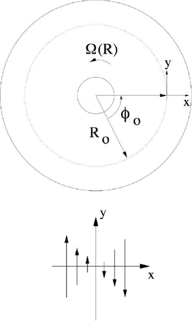
Figure 1.3: Local coordinate system at $t=0$.

The resulting equations of motion for a fluid in the local model (including self-gravity) are

$$\partial_{t}\mbox{\boldmath$v$}+(\mbox{\boldmath$v$}\cdot\mbox{\boldmath$\nabla$})\mbox{\boldmath$v$}=-\frac{1}{\Sigma}\mbox{\boldmath$\nabla$}\left(P+\frac{B^{2}}{8\pi}\right)+\frac{({\mbox{\boldmath$B$}}\cdot\mbox{\boldmath$\nabla$}){\mbox{\boldmath$B$}}}{4\pi\rho}-\mbox{\boldmath$\nabla$}\phi-2\mbox{\boldmath$\Omega$}{\bf\times}\mbox{\boldmath$v$}+3\Omega^{2}x\hat{\mbox{\boldmath$x$}},$$ (1.18)

where $v$ is the fluid velocity with respect to the rotating frame, $B$ is the magnetic field, $P$ is the two-dimensional pressure, $\Sigma$ is the column density and $\phi$ is the disk potential with the time-steady axisymmetric component removed. The last two terms on the right-hand side of equation (1.18) incorporate the effects of Coriolis and centrifugal forces as well as the gravitational acceleration due to the central point mass and the time-steady axisymmetric component of the disk. These equations of motions are valid for a disk system in which the gravitational potential is dominated by the central object; the fluid in such a disk follows a Keplerian rotation curve, $v_{\phi}\sim r^{-1/2}$.

The continuity, internal energy and induction equations retain their usual form:

$$\partial_{t}\Sigma+(\mbox{\boldmath$v$}\cdot\mbox{\boldmath$\nabla$})\Sigma+\Sigma\mbox{\boldmath$\nabla$}\cdot\mbox{\boldmath$v$}=0,$$ (1.19)

$$\partial_{t}U+(\mbox{\boldmath$v$}\cdot\mbox{\boldmath$\nabla$})U+(U+P)\mbox{\boldmath$\nabla$}\cdot\mbox{\boldmath$v$}+\Lambda=0,$$ (1.20)

(where $U$ is the internal energy per unit area and $\Lambda$ is the cooling function) and

$$\partial_{t}{\mbox{\boldmath$B$}}-\mbox{\boldmath$\nabla$}{\bf\times}(\mbox{\boldmath$v$}{\bf\times}{\mbox{\boldmath$B$}})=0.$$ (1.21)

Equations (1.18) through (1.21) are the equations of compressible ideal magnetohydrodynamics (MHD) in the local model. Magnetic fields are assumed to be dynamically unimportant for most of research described in this dissertation, in which case equations (1.18) through (1.20) reduce to the equations of compressible hydrodynamics. The disk self-gravity ($\phi$ in equation [1.18]) and explicit cooling ($\Lambda$ in equation [1.20]) are neglected except in the work discussed in Chapter 2. In Chapters 2 - 4, the fluid is assumed to obey an ideal-gas equation of state, $P=(\gamma-1)U$, where $\gamma$ is the adiabatic index. Chapter 5 assumes an isothermal equation of state $P=c_{s}^{2}\Sigma$.

With constant density and pressure in equilibrium, an exact steady-state solution to equations (1.18) through (1.20) is $\mbox{\boldmath$v$}_{o}=-\frac{3}{2}\Omega x\hat{\mbox{\boldmath$y$}}$. This uniform shear velocity is a manifestation of differential rotation of the fluid in the disk. As a result, the (two-dimensional) local model is referred to as the “shearing sheet”. The numerical implementation of the shearing sheet requires a careful treatment of the boundary conditions in the radial direction. These boundary conditions are described in detail in Hawley et al. [1995]. In brief, one uses strictly periodic boundary conditions in $y$ and shearing-periodic boundary conditions in $x$. The latter is done by enforcing periodic boundary conditions in the radial direction followed by an advection of the boundary fluid due to the shear. This assumes that the shearing sheet is surrounded by identical boxes that are strictly periodic initially, with a large-scale shear flow present across all the boxes.

The shearing-sheet equations are evolved using a ZEUS-based scheme [Stone and Norman, 1992]: a time-explicit, operator-split, finite-difference method on a staggered grid which uses an artificial viscosity to capture shocks. An important modification of the standard shearing sheet, introduced by Masset [2000], is the splitting of the overall shear velocity from the rest of the flow. This overcomes a practical limitation of the standard shearing sheet, which is the small Courant-limited time step imposed by the large shear velocities at the edges of the sheet; for numerical stability of grid-based schemes the Courant condition requires time steps to be lower than the grid spacing divided by the maximum velocity on the grid. The larger the box, the more severe this limitation becomes. Separating out the shear removes this limitation and allows one to increase the size of the shearing sheet arbitrarily. This separation is done by replacing $v_{y}$ by $v_{o}+\delta v_{y}$ in the fluid equations, and then evolving $\delta v_{y}$; this can be done because there is no evolution of $v_{o}$ directly ($\partial_{t}v_{o}=0$ and $\mbox{\boldmath$\nabla$}v_{o}={\rm{constant}}$). Advection of other fluid variables by $v_{o}$ is done by splitting the distance over which the fluid is sheared into an integral and fractional number of grid zones: the fluid variables are simply shifted an integral number of zones and then advected in the usual manner for the remaining fractional part (which does not require a higher effective velocity than any other part of the flow).

1.6 Discussion

While a rigorous proof of the stability of weakly-ionized disks may well be impossible, the results of this dissertation add to the already strong evidence against a turbulent angular momentum transport mechanism in weakly-ionized disks. Gravitational instability likely results in fragmentation, radial convection is suppressed by differential rotation and two-dimensional vortices, which provide a decaying flux of angular momentum, are likely to be unstable in three dimensions. Evidence against a local, nonlinear, purely hydrodynamic instability is mounting.

Accretion may be driven globally by a magneto-centrifugal wind [Blandford and Payne, 1982] or tidally-induced spiral waves [Larson, 1989, Livio and Spruit, 1991], or locally via spiral waves excited by planets embedded in the disk [Goodman and Rafikov, 2001, Sari and Goldreich, 2004]. There also exist global instabilities (e.g., Papaloizou and Pringle 1984, 1985) that result in a small amount of turbulence and angular momentum transport (e.g., Hawley 1987). In addition, there are instabilities associated with the dust layer in YSO disks (e.g., Garaud and Lin 2004) that will generate some amount of turbulence in those systems. While one or more of these mechanisms may play a role in transporting angular momentum in certain systems, their dependence upon global structure or other special features in order to operate makes their broad application to weakly-ionized disks doubtful. Alternatively, weakly-ionized disks may simply be inactive except in ionized surface layers [Gammie, 1996].

A detailed discussion of these possibilities is beyond the scope of this dissertation, but a brief discussion of layered accretion is given in Chapter 6, along with some proposals for future modeling based upon that idea. Chapter 6 also summarizes the main results and implications of this work, and provides some direction as to where to go from here in the search for a turbulent angular momentum transport mechanism in weakly-ionized accretion disks. In addition, proposals are made for future investigations of the properties of turbulent stresses in ionized disks, with a view towards incorporating these properties in advanced, physically-motivated disk models.

Chapter 2 Nonlinear Outcome of Gravitational Instability in Disks with Realistic Cooling

2.1 Chapter Overview

We consider the nonlinear outcome of gravitational instability in optically-thick disks with a realistic cooling function. We use a numerical model that is local, razor-thin, and unmagnetized. External illumination is ignored. Cooling is calculated from a one-zone model using analytic fits to low temperature Rosseland mean opacities. The model has two parameters: the initial surface density $\Sigma_{o}$ and the rotation frequency $\Omega$. We survey the parameter space and find: (1) The disk fragments when ${{\langle}{\langle}\tau_{c}{\rangle}{\rangle}}\Omega\sim 1$, where ${{\langle}{\langle}\tau_{c}{\rangle}{\rangle}}$ is an effective cooling time defined as the average internal energy of the model divided by the average cooling rate. This is consistent with earlier results that used a simplified cooling function. (2) The initial cooling time ${\tau_{co}}$ for a uniform disk with Toomre stability parameter $Q=1$ can differ by orders of magnitude from ${{\langle}{\langle}\tau_{c}{\rangle}{\rangle}}$ in the nonlinear outcome. The difference is caused by sharp variations in the opacity with temperature. The condition ${\tau_{co}}\Omega\sim 1$ therefore does not necessarily indicate where fragmentation will occur. (3) The largest difference between ${{\langle}{\langle}\tau_{c}{\rangle}{\rangle}}$ and ${\tau_{co}}$ is near the opacity gap, where dust is absent and hydrogen is largely molecular. (4) In the limit of strong illumination the disk is isothermal; we find that an isothermal version of our model fragments for $Q\lesssim 1.4$. Finally, we discuss some physical processes not included in our model, and find that most are likely to make disks more susceptible to fragmentation. We conclude that disks with ${{\langle}{\langle}\tau_{c}{\rangle}{\rangle}}\Omega\lesssim 1$ do not exist.

2.2 Introduction

The outer regions of accretion disks in both active galactic nuclei (AGN) and young stellar objects (YSO) are close to gravitational instability (for a review see, for AGN: Shlosman et al. 1990; YSOs: Adams and Lin 1993). Gravitational instability can be of central importance in disk evolution. In some disks, it leads to the efficient redistribution of mass and angular momentum (e.g. Larson 1984, Laughlin and Rozyczka 1996, Gammie 2001). In other disks, gravitational instability leads to fragmentation and the formation of bound objects. This may cause the truncation of circumnuclear disks [Goodman, 2003], or the formation of planets (e.g. Boss 1997, and references therein).

We will restrict attention to disks whose potential is dominated by the central object, and whose rotation curve is therefore approximately Keplerian. Gravitational instability to axisymmetric perturbations sets in when the sound speed $c_{s}$, the rotation frequency $\Omega$, and the surface density $\Sigma$ satisfy

$$Q\equiv{\frac{c_{s}\Omega}{\pi G\Sigma}}<Q_{crit}\simeq 1$$ (2.1)

[Toomre, 1964, Goldreich and Lynden-Bell, 1965]. Here $Q_{crit}=1$ for a “razor-thin” (two- dimensional) fluid disk model of the sort we will consider below, and $Q_{crit}=0.676$ for a finite-thickness isothermal disk [Goldreich and Lynden-Bell, 1965]. The instability condition (2.1) can be rewritten, for a disk with scale height $H\simeq c_{s}/\Omega$, around a central object of mass $M_{*}$,

$$M_{disk}\gtrsim\frac{H}{r}M_{*},$$ (2.2)

where $M_{disk}=\pi r^{2}\Sigma$. For YSO disks $H/r\sim 0.1$ and thus a massive disk is required for instability. AGN disks are expected to be much thinner. The instability condition can be rewritten in a third, useful form if we assume that the disk is in a steady state and its evolution is controlled by internal (“viscous”) transport of angular momentum. Then the accretion rate $\dot{M}=3\pi\alpha c_{s}^{2}\Sigma/\Omega$, where $\alpha\lesssim 1$ is the usual dimensionless viscosity of Shakura and Sunyaev [1973], and

$$\dot{M}\gtrsim\frac{3\alpha c_{s}^{3}}{G}=7.1\times 10^{-4}\,\alpha\left(\frac{c_{s}}{1{\rm\,km\,s^{-1}}}\right)^{3}\,{M_{\odot}}{\rm\,yr}^{-1}$$ (2.3)

implies gravitational instability (e.g. Shlosman et al. [1990]). Disks dominated by external torques (e.g. a magnetohydrodynamic [MHD] wind) can have higher accretion rates (but not arbitrarily higher; see Goodman 2003) while avoiding gravitational instability.

For a young, solar-mass star accreting from a disk with $\alpha=10^{-2}$ at $10^{-6}{M_{\odot}}{\rm\,yr}^{-1}$, equation (2.3) implies that instability occurs where the temperature drops below $17{\rm\,K}$. Disks may not be this cold if the star is located in a warm molecular cloud where the ambient temperature is greater than $17{\rm\,K}$, or if the disk is bathed in scattered infrared light from the central star (although there is some evidence for such low temperatures in the solar nebula, e.g. Owen et al. 1999). If the vertically-averaged value of $\alpha$ is small and internal dissipation is confined to surface layers, as in the layered accretion model of Gammie [1996], then instability can occur at higher temperatures, although equation (2.2) still requires that the disk be massive.

AGN disk heating is typically dominated by illumination from a central source. The temperature then depends on the shape of the disk. If the disk is flat or shadowed, however, and transport is dominated by internal torques, one can apply equation (2.3). For example, in the nucleus of NGC 4258 [Miyoshi et al., 1995] the accretion rate may be as large as $10^{-2}{M_{\odot}}{\rm\,yr}^{-1}$ [Lasota et al., 1996, Gammie et al., 1999]. Equation (2.3) then implies that instability sets in where $T<10^{4}(\alpha/10^{-2}){\rm\,K}$. If the disk is illumination-dominated then $Q$ fluctuates with the luminosity of the central source.

In a previous paper [Gammie, 2001], one of us investigated the effect of gravitational instability in cooling, gaseous disks in a local model. A simplified cooling function $\Lambda$ was employed in these simulations, with a fixed cooling time ${\tau_{co}}$:

$$\Lambda=-\frac{U}{{\tau_{co}}},$$ (2.4)

where $U\equiv$ the internal energy per unit area. Disk fragmentation was observed for ${\tau_{co}}\Omega\lesssim 3$. The purpose of this paper is to investigate gravitational instability in a local model with more realistic cooling.

Several recent numerical experiments have included cooling, as opposed to isothermal or adiabatic evolution, and we can ask whether these results are consistent with Gammie [2001]. Nelson et al. [2000] studied a global two-dimensional (thin) SPH model in which the vertical density and temperature structure is calculated self-consistently and each particle radiates as a blackbody at the surface of the disk. The initial conditions at a radius corresponding to the minimum initial value of Q ($\sim 1.5$) for these simulations were $\Sigma_{o}\approx 50{\rm\,g\,cm^{-2}},\Omega\approx 8\times 10^{-10}{\rm\,s^{-1}}$; the initial cooling time under these circumstances is ${\tau_{co}}\approx 250\,\Omega^{-1}$, so fragmentation is not expected and is not observed.

Durisen et al. [2001] consider a global three dimensional (3D) Eulerian hydrodynamics model in which the volumetric cooling rate varies with height above the midplane so as to preserve an isentropic vertical structure. The cooling time is fixed at each radius. Their cooling time $\gtrsim 10\Omega^{-1}$ at all radii, so fragmentation is not expected based on the criterion of Gammie [2001]. The simulations show structure formation due to gravitational instabilities but not fragmentation.

Rice et al. [2003] consider a global 3D SPH model with a cooling time that is a fixed multiple of $\Omega^{-1}(r)$. They find that their disk fragments when ${\tau_{co}}\approx 3\Omega^{-1}$ and $M_{disk}=0.1M_{*}$. For a more massive disk ($M_{disk}=0.25M_{*}$), fragmentation occurred at somewhat higher cooling times (${\tau_{co}}\approx 10\Omega^{-1}$). This is effectively a global generalization of the local model problem considered by Gammie [2001]. The fact that the results are so consistent suggests that the local, thin approximation used in Gammie [2001] and here give a reasonable approximation to a global outcome.

Mayer et al. [2002] consider a global three dimensional SPH model of a circumstellar disk. Explicit cooling is not included, but the equation of state switches from isothermal to adiabatic when gravitational instability begins to set in. This is designed to account for the inefficient cooling of dense, optically thick regions. Fragmentation is observed. Realistic cooling can have a complex influence on disk evolution, and it is not clear that switching between isothermal and adiabatic behavior “brackets” the outcomes that might be obtained when full cooling is used.

Other notable recent work, such as that by Boss [2002], includes strong radiative heating in the sense that the effective temperature of the external radiation field $T_{irr}$ is comparable to or larger than the disk midplane temperature $T_{c}$. In the limit that $T_{irr}\ll T_{c}$ we recover the limit considered here and in Gammie [2001]; in the limit that $T_{irr}\gg T_{c}$ the disk is effectively isothermal.

The plan of this paper is as follows. In §2.3 we describe the model, with a detailed description of the cooling function given in §2.4. The results of numerical experiments are described in §2.5. Conclusions are given in §2.6.

2.3 Model

The model we use here is identical to that used in Gammie [2001] in every respect except that we use a more complicated cooling function. To make the description more self-contained, we summarize the basic equations of the model here. The model is local, in the sense that it considers a region of size $L$ where $L/r_{o}\ll 1$ and $r_{o}$ is a fiducial radius. We use a local Cartesian coordinate system $x\equiv r-r_{o}$ and $y\equiv(\phi-\Omega t)r_{o}$, where $r,\phi$ are the usual cylindrical coordinates and $\Omega$ is the orbital frequency at $r_{o}$. The model is also thin in the sense that matter is confined entirely to the plane of the disk.

Using the local approximation one can perform a formal expansion of the equations of motion in the small parameter $L/r_{o}$. The resulting equations of motion read, where $v$ is the velocity, $P$ is the (two-dimensional) pressure, and $\phi$ is the gravitational potential with the time-steady axisymmetric component removed:

$$\frac{D\mbox{\boldmath$v$}}{Dt}=-\frac{\mbox{\boldmath$\nabla$}P}{\Sigma}-2\mbox{\boldmath$\Omega$}\times\mbox{\boldmath$v$}+3\Omega^{2}x\hat{\mbox{\boldmath$x$}}-\mbox{\boldmath$\nabla$}\phi.$$ (2.5)

For constant pressure and surface density, $\mbox{\boldmath$v$}=-\frac{3}{2}\Omega x\hat{\mbox{\boldmath$y$}}$ is an equilibrium solution to the equations of motion. This linear shear flow is the manifestation of differential rotation in the local model.

The equation of state is

$$P=(\gamma-1)U,$$ (2.6)

where $P$ is the two-dimensional pressure and $U$ the two-dimensional internal energy. The two-dimensional (2D) adiabatic index $\gamma$ can be mapped to a 3D adiabatic index $\Gamma$ in the low-frequency (static) limit. For a non-self-gravitating disk $\gamma=(3\Gamma-1)/(\Gamma+1)$ (e.g. Goldreich et al. 1986, Ostriker et al. 1992). For a strongly self-gravitating disk, one can show that $\gamma=3-2/\Gamma$. We adopt $\Gamma=7/5$ throughout, which yields $\gamma=11/7$.

The internal energy equation is

$$\frac{\partial U}{\partial t}+\nabla\cdot(U\mbox{\boldmath$v$})=-P\mbox{\boldmath$\nabla$}\cdot\mbox{\boldmath$v$}-\Lambda,$$ (2.7)

where $\Lambda=\Lambda(\Sigma,U,\Omega)$ is the cooling function, fully described below. Notice that there is no heating term; heating is due solely to shocks. Numerically, entropy is increased by artificial viscosity in shocks.

The gravitational potential is determined by the razor-thin disk Poisson equation:

$$\nabla^{2}\phi=4\pi G\Sigma\,\delta(z).$$ (2.8)

For a single Fourier component of the surface density $\Sigma_{\mbox{\boldmath$k$}}$ this has the solution

$$\phi=-\frac{2\pi G}{|\mbox{\boldmath$k$}|}\Sigma_{\mbox{\boldmath$k$}}e^{i\mbox{\boldmath$k$}\cdot{\bf x}-|kz|}.$$ (2.9)

A finite-thickness disk has weaker self-gravity, but this does not qualitatively change the dynamics of the disk in linear theory [Goldreich and Lynden-Bell, 1965].

We integrate the governing equations using a self-gravitating hydrodynamics code based on ZEUS [Stone and Norman, 1992]. ZEUS is a time-explicit, operator-split, finite-difference method on a staggered mesh. It uses an artificial viscosity to capture shocks. Our implementation has been tested on standard linear and nonlinear problems, such as sound waves and shock tubes. We use the “shearing box” boundary conditions, described in detail by Hawley et al. [1995], and solve the Poisson equation using the Fourier transform method, modified for the shearing box boundary conditions. See Gammie [2001] for further details on boundary conditions, numerical methods and tests.

The numerical model is always integrated in a region of size $L\times L$ at a numerical resolution of $N\times N$. In linear theory the disk is most responsive at the critical wavelength $2c_{s}^{2}/G\Sigma_{o}$. We have checked the dependence of the outcome on $L$ and found that as long as $L\gtrsim 2c_{s}^{2}/G\Sigma_{o}$ the outcome does not depend on $L$. We have also checked the dependence of the outcome on $N$ and found that the outcome is insensitive to $N$, at least for the models with $N\geq 256$ that we use.

2.4 Cooling Function

Our cooling function is determined from a one-zone model for the vertical structure of the disk. The disk cools at a rate per unit area

$$\Lambda\equiv 2\sigma T_{e}^{4},$$ (2.10)

which defines the effective temperature $T_{e}$. The cooling function depends on the heat content of the disk and how that content is transported from the disk interior to the surface: by radiation, convection, or perhaps some more exotic form of turbulent transport such as MHD waves. Low temperature disks are expected to be convectively unstable (e.g. Cameron 1978, Lin and Papaloizou 1980). Cassen [1993] has argued, however, that the radiative heat flux in an adiabatically-stratified disk is comparable to the heat dissipated by turbulence (in an $\alpha$-disk model), suggesting that convection is incapable of radically altering the vertical structure of the disk. We will consider only radiative transport.

If the disk is optically thick in the Rosseland mean sense, so that radiative transport can be treated in the diffusion approximation, then [Hubeny, 1990]

$$T_{e}^{4}=\frac{8}{3}\frac{T_{c}^{4}}{\tau}$$ (2.11)

where $\tau$ is the Rosseland mean optical depth and $T_{c}$ is the central temperature. We will assume that $T_{c}\approx T$, where

$$T=\frac{\mu m_{p}c_{s}^{2}}{\gamma k_{B}},$$ (2.12)

and

$$c_{s}^{2}=\gamma(\gamma-1)\frac{U}{\Sigma},$$ (2.13)

which follows from the equation of state and the assumption that the radiation pressure is small (we have verified that this is never seriously violated). Here $k_{B}$ is Boltzmann’s constant, $m_{p}$ is the proton mass, and $\mu$ is the mean mass per particle, which we have set to $2.4$ in models with initial temperature below the boundary between the grain-evaporation opacity and molecular opacity and $\mu=0.6$ in models with initial temperature above the boundary.

The optical depth is

$$\tau\equiv\int_{0}^{\infty}\,dz\,\kappa(\rho_{z},T_{z})\rho_{z}$$ (2.14)

where $\kappa$ is the Rosseland mean opacity, $\rho_{z}$ and $T_{z}$ are local density and temperature, and $z$ is the height above the midplane. Following the usual one-zone approximation,

$$\int_{0}^{\infty}\,dz\,\kappa(\rho_{z},T_{z})\rho_{z}\approx H\kappa(\bar{\rho},\bar{T})\bar{\rho}$$ (2.15)

where the overbar indicates a suitable average and $H\approx c_{s}(T)/\Omega$ is the disk scale height (we ignore the effects of self-gravity on the disk scale height, which is valid when locally $Q\gtrsim 1$). Taking $\bar{T}\approx T$ and $\bar{\rho}\approx\Sigma/(2H)$ then gives a final, closed expression for $\Lambda$.

We have adopted the analytic approximations to the opacities provided by Bell and Lin [1994]. These opacities are dominated by, in order of increasing temperature: grains with ice mantles, grains without ice mantles, molecules, H^- scattering, bound-free/free-free absorption and electron scattering. The molecular opacity regime is commonly called the opacity gap; it is too hot for dust, but too cold for H^- scattering to contribute much opacity. The opacity can be as much as $4$ orders of magnitude smaller than the $\sim 5{\rm\,g}{\rm\,cm}^{-2}$ typical of the dust-dominated opacity regime. It turns out that this feature plays a significant role in the evolution of gravitationally-unstable disks.

To sum up, the cooling function is

$$\Lambda(\Sigma,U,\Omega)=\frac{16}{3}\frac{\sigma T^{4}}{\tau}.$$ (2.16)

For a power-law opacity of the form $\kappa=\kappa_{0}\rho^{a}T^{b}$, this implies that

$$\Lambda\sim\Sigma^{-5-3a/2+b}U^{4+a/2-b}.$$ (2.17)

From this it follows that the cooling time ${\tau_{c}}\equiv U/\Lambda$ scales as

$${\tau_{c}}\sim\Sigma^{5+3a/2-b}U^{-3-a/2+b}.$$ (2.18)

If the disk evolves quasi-adiabatically (as it does if the cooling time is long compared to the dynamical time) then $U\sim\Sigma^{\gamma}$ and

$${\tau_{c}}\sim\Sigma^{5-3\gamma+(a/2)(3-\gamma)+b(\gamma-1)}.$$ (2.19)

Table 2.1: Scaling Exponent for Cooling Time as a Function of Surface Density

Opacity Regime	a	b	Exponent
Ice grains	0	2	10/7
Evaporation of ice grains	0	-7	-26/7
Metal grains	0	1/2	4/7
Evaporation of metal grains	1	-24	-89/7
Molecules	2/3	3	52/21
H- scattering	1/3	10	131/21
Bound-free and free-free	1	-5/2	-3/7
Electron scattering	0	0	2/7

Table 2.1 gives a list of values for this scaling exponent for our nominal value of $\gamma=11/7$. Notice that, when ice grains or metal grains are evaporating, and in the bound-free/free-free opacity regime, cooling time decreases as surface density increases.

Our cooling function is valid in the limit of large optical depth ($\tau\gg 1$). Since the disk becomes optically thin at some locations in the course of a typical run, we must modify this result so that the cooling rate does not diverge at small optical depth. A modification that produces the correct asymptotic behavior is

$$\Lambda=\frac{16}{3}\sigma T^{4}\frac{\tau}{1+\tau^{2}}.$$ (2.20)

This interpolates smoothly between the optically-thick and optically-thin regimes and is proportional to the (Rosseland mean) optical depth in the optically-thin limit. While it would be more physically sensible to use a Planck mean opacity in the optically-thin limit, usually the optically-thin regions contain little mass so their cooling is not energetically significant. An exception is in the opacity gap, where even high density regions become optically thin.

Our simulations begin with $\Sigma$ and $U$ constant. The velocity field is perturbed from the equilibrium solution to initiate the gravitational instability. The initial velocities are $v_{x}=\delta v_{x}$, $v_{y}=-\frac{3}{2}\Omega x+\delta v_{y}$, where $\delta\mbox{\boldmath$v$}$ is a Gaussian random field of amplitude ${\langle}\delta v^{2}{\rangle}/c_{s}^{2}=0.1$. The power spectrum of perturbations is white noise ($v_{k}^{2}\sim k^{0}$) in a band in wavenumber $k_{crit}/4<|k|<4k_{crit}$ surrounding the minimum $k_{crit}=1/(\pi Q^{2})$ (with $G=\Sigma_{o}=\Omega=1$) in the density-wave dispersion relation. We have checked in particular cases that for $10^{-3}<{\langle}\delta v^{2}{\rangle}/c_{s}^{2}<10$ the outcome is qualitatively unchanged. This is expected because disk perturbations (unlike cosmological perturbations) grow exponentially and the initial conditions are soon forgotten.

Excluding the initial velocity field, the initial conditions for a spatially-uniform disk consist of three parameters: $\Sigma_{o},U_{o}$, and $\Omega$. We fix $Q=1$, leaving two degrees of freedom. In models with simple, scale-free cooling functions such as that considered by Gammie [2001], these degrees of freedom remain and can be scaled away by setting $G=\Sigma_{o}=\Omega=1$. That is, there is a two-dimensional continuum of disks (with varying values of $\Sigma_{o}$ and $\Omega$, but the same value of $Q$) that are described by a single numerical model.

The opacity contains definite physical scales in density and temperature. The realistic cooling function considered here therefore removes our freedom to rescale the disk surface density and rotation frequency. That is, there is now a one-to-one correspondence between disks with fixed $\Sigma$ and $\Omega$ and our numerical models.

The choice of $\Sigma_{o}$ and $\Omega$ as labels for the parameter space is not unique. Internally in the code we fix the initial volume density (in ${\rm\,g\,cm^{-3}}$) and the initial temperature (in Kelvins). These choices are difficult to interpret, however, since they are tied to quantities that change over the course of the simulation; $\Omega$ and the mean value of $\Sigma$ do not.

The cooling is integrated explicitly using a first-order scheme. The timestep is modified to satisfy the Courant condition and to be less than a fixed fraction of the shortest cooling time on the grid. We have varied this fraction and shown that the results are insensitive to it, provided that it is sufficiently small.

2.5 Nonlinear Outcome

2.5.1 Standard Run

Consider the evolution of a single “standard” run, with $\Sigma_{o}=1.4\times 10^{5}{\rm\,g}{\rm\,cm}^{-2}$ and $\Omega=1.1\times 10^{-7}\sec^{-1}$. This corresponds to $T_{o}=1200$ and ${\tau_{co}}=9.0\times 10^{4}\Omega^{-1}$. The model size is $L=320G\Sigma_{o}/\Omega^{2}$ and numerical resolution $1024^{2}$. The model initially lies at the lower edge of the opacity gap.

The evolution of the kinetic, gravitational and thermal energy per unit area (${\langle}E_{k}{\rangle}$, ${\langle}E_{g}{\rangle}$ and ${\langle}E_{th}{\rangle}$ respectively) normalized to $G^{2}\Sigma_{o}^{3}/\Omega^{2}$, are shown in Figure 2.1. After the initial phase of gravitational instability the model settles into a statistically-steady, gravito-turbulent state. It does not fragment. Cooling is balanced by shock heating. Energy for driving the shocks is extracted from the shear flow, and the mean shear flow is enforced by the boundary conditions.

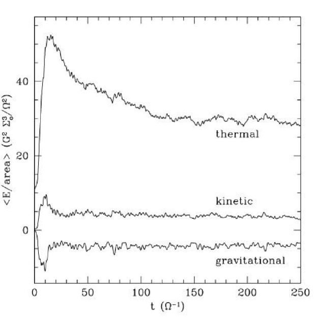
Figure 2.1: Evolution of the kinetic, gravitational, and thermal energy per unit area, normalized to $G^{2}\Sigma_{o}^{3}/\Omega^{2}$, in the standard run, which has $L=320G\Sigma_{o}/\Omega^{2}$, resolution $1024^{2}$, and ${\tau_{co}}=9.0\times 10^{4}\Omega^{-1}$.

The turbulent state transports angular momentum outward via hydrodynamic and gravitational shear stresses. The dimensionless gravitational shear stress is

$$\alpha_{grav}=\frac{1}{{\langle}\frac{3}{2}\Sigma c_{s}^{2}{\rangle}}\int_{-\infty}^{\infty}dz\frac{g_{x}g_{y}}{4\pi G}$$ (2.21)

where ${\bf g}$ is the gravitational acceleration, and the dimensionless hydrodynamic shear stress is

$$\alpha_{hyd}=\frac{\Sigma v_{x}\delta v_{y}}{{\langle}\frac{3}{2}\Sigma c_{s}^{2}{\rangle}}$$ (2.22)

where ${\langle}{\rangle}$ denote a spatial average. Figure 2.2 shows the evolution of ${\langle}\alpha_{grav}{\rangle}$ and ${\langle}\alpha_{hyd}{\rangle}$ in the standard run. Averaged over the last $230\Omega^{-1}$ of the run, ${\langle}{\langle}\alpha_{hyd}{\rangle}{\rangle}=0.0079$, ${\langle}{\langle}\alpha_{grav}{\rangle}{\rangle}=0.017$, and so the total dimensionless shear stress is ${\langle}{\langle}\alpha{\rangle}{\rangle}=0.025$, where ${\langle}{\langle}{\rangle}{\rangle}$ denote a space and time average.

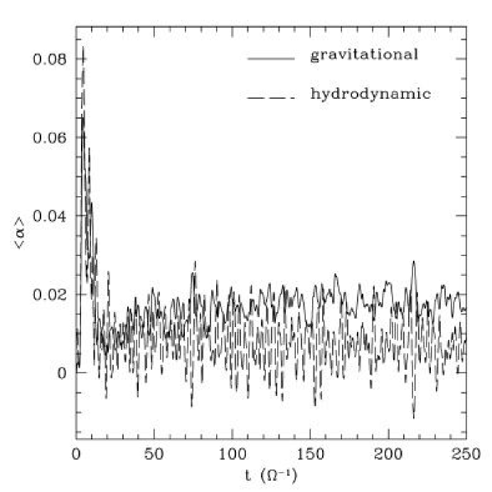
Figure 2.2: Evolution of the gravitational and hydrodynamic pieces of ${\langle}\alpha{\rangle}$ in the standard run.

The mean stability parameter ${\langle}Q{\rangle}\equiv\langle c_{s}\rangle\Omega/\pi G\langle\Sigma\rangle$ averages $1.86$ over the last $230\Omega^{-1}$ of the run. Because the temperature and surface density vary strongly, other methods of averaging $Q$ will give different results.

Figure 2.3 shows a snapshot of the surface density at $t=50\Omega^{-1}$. The structure is similar to that observed in Gammie [2001], with trailing density structures. The density structures are stretched into a trailing configuration by the prevailing shear flow. Their scale is determined by the disk temperature and surface density rather than the size of the box (see Gammie 2001).

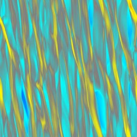
Figure 2.3: Map of surface density at $t=50\Omega^{-1}$ in the standard run. Dark shades (blue in color version) indicate low density ($0.2\Sigma_{o}$) and light shades (yellow in color version) indicate high density ($3\Sigma_{o}$).

2.5.2 Varying $\Sigma_{o}$ and $\Omega$

We now turn to exploring the two-dimensional parameter space of models. First consider a series of models with the same initial central temperature, but with varying ${\tau_{co}}$. As ${\tau_{co}}$ is lowered the time-averaged gravitational potential energy per unit area ${\langle}{\langle}E_{g}{\rangle}{\rangle}$ increases monotonically in magnitude. The gravito-turbulent state becomes more extreme, with larger ${\langle}{\langle}\alpha{\rangle}{\rangle}$, larger perturbed velocities, and larger density contrasts. Eventually a threshold is crossed and the disk fragments.

Fragmentation is illustrated in Figure 2.5, which shows a snapshot from a run with $\Sigma_{o}=6.6\times 10^{3}{\rm\,g}{\rm\,cm}^{-2}$, $\Omega=5.4\times 10^{-9}\sec^{-1}$. This corresponds to $T_{o}=1200$, ${\tau_{co}}=0.025\Omega^{-1}$. The run has numerical resolution $256^{2}$ and $L=80G\Sigma_{o}/\Omega^{2}$. The largest bound object in the center of the figure was formed from the collision and coalescence of several smaller bound objects. A snapshot of the optical depth at the same point in the simulation is given in Figure 2.5. For each snapshot, red indicates high values of the mapped variable and blue indicates low values. Much of the disk is optically thick, but most of the low density regions are optically thin in the Rosseland mean sense.

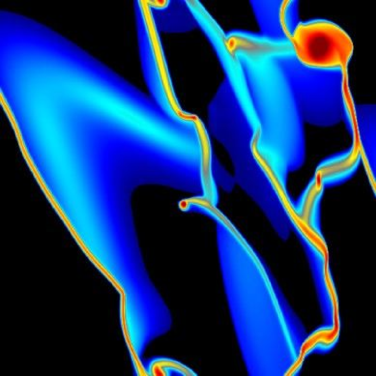
Figure 2.4: Map of surface density in a run with ${\tau_{co}}=0.025\Omega^{-1}$. Dark shades indicate both low density ($10^{-2}\Sigma_{0}$, black in color version) and high density ($10^{2}\Sigma_{0}$, near the centers of bound objects, red in color version).

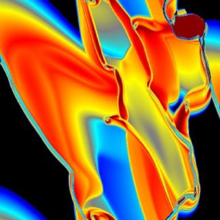
Figure 2.5: Map of optical depth $\tau$ in a run with ${\tau_{co}}=0.025\Omega^{-1}$. Dark shades indicate both low $\tau$ ($10^{-2}$, black in color version) and high $\tau$ ($10^{4}$, near the centers of bound objects, red in color version).

Lowering ${\tau_{co}}$ sufficiently always leads to fragmentation. We have surveyed the parameter space of $\Omega$ and $\Sigma_{o}$ to determine where the disk begins to fragment. Each model was run to $100\Omega^{-1}$. Figures 2.7 and 2.7 summarize the results. Two heavy solid lines are shown on each diagram. The upper line shows the most rapidly cooling simulations that show no signs of gravitational fragmentation (nonfragmentation point). Quantitatively, we define this as the point at which the time-averaged gravitational potential energy per unit area is equal to $-3G^{2}\Sigma_{o}^{3}/\Omega^{2}$. The lower line shows the most slowly cooling simulations to show definite fragmentation (fragmentation point). Quantitatively, we define this as the point at which the gravitational potential energy per unit area

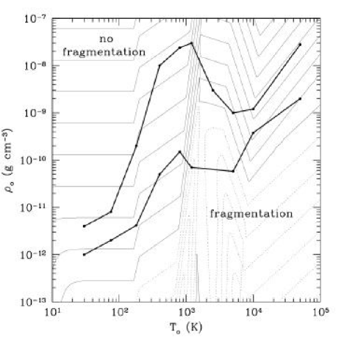
Figure 2.6: Location of the critical curves as a function of initial volume density and temperature (in cgs units). Each contour line is an order of magnitude change in ${\tau_{co}}$, solid/dotted lines indicating positive/negative integer values of log(${\tau_{co}}$).

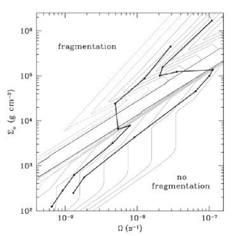
Figure 2.7: Location of the critical curves as a function of initial surface density and rotation frequency (in cgs units). Each contour line is an order of magnitude change in ${\tau_{co}}$, solid/dotted lines indicating positive/negative integer values of log(${\tau_{co}}$). The gap in the center of the plot is due to the discontinuous jump in the value of $\mu$.

is equal to $-300G^{2}\Sigma_{o}^{3}/\Omega^{2}$ at some point during the run. Figure 2.7 shows the data in the $\rho_{o},T_{o}$ plane, while Figure 2.7 shows the results in the $\Sigma_{o},\Omega$ plane. Light contours are lines of constant ${\tau_{co}}$.

The transition from persistent, gravito-turbulent outcomes to fragmentation is gradual and statistical in nature. Figure 2.8 shows the gravitational potential energy per unit area in the transition region for a series of runs with $T_{o}=1200{\rm\,K}$. The abscissa is labeled with the initial cooling time ${\tau_{co}}\Omega$. There is a gradual, approximately logarithmic increase in the magnitude of ${\langle}{\langle}E_{g}{\rangle}{\rangle}$ as ${\tau_{co}}$ decreases. Runs in this region exhibit the transient formation of small bound objects which might collapse if additional physics (e.g. the effects of MHD turbulence) were included in the model. Eventually $-{\langle}{\langle}E_{g}{\rangle}{\rangle}$ begins to increase dramatically, and we define the transition point as the beginning of this steep increase in gravitational binding energy.

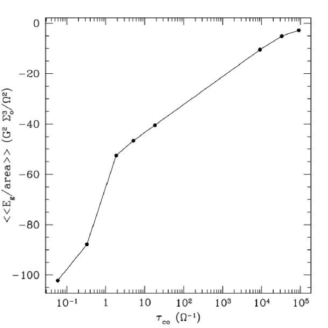
Figure 2.8: Mean gravitational potential energy as a function of initial cooling time for a series of models with varying initial cooling time and $T_{o}=1200$.

Figure 2.9 shows the run of ${\tau_{co}}\Omega$ for the fragmentation point, transition point, and nonfragmentation point as a function of $T_{o}$. It is surprising that a disk can begin to exhibit signs of gravitational collapse for ${\tau_{co}}\Omega$ as large as $10^{6}$, and evade collapse for ${\tau_{co}}\Omega$ as small as $0.02$. A naive application of the results of Gammie [2001] would suggest that fragmentation should occur for ${\tau_{co}}\Omega\lesssim 3$. Evidently this estimate can be off by orders of magnitude, with the largest error for $T_{o}\approx 10^{3}{\rm\,K}$, just below the opacity gap.

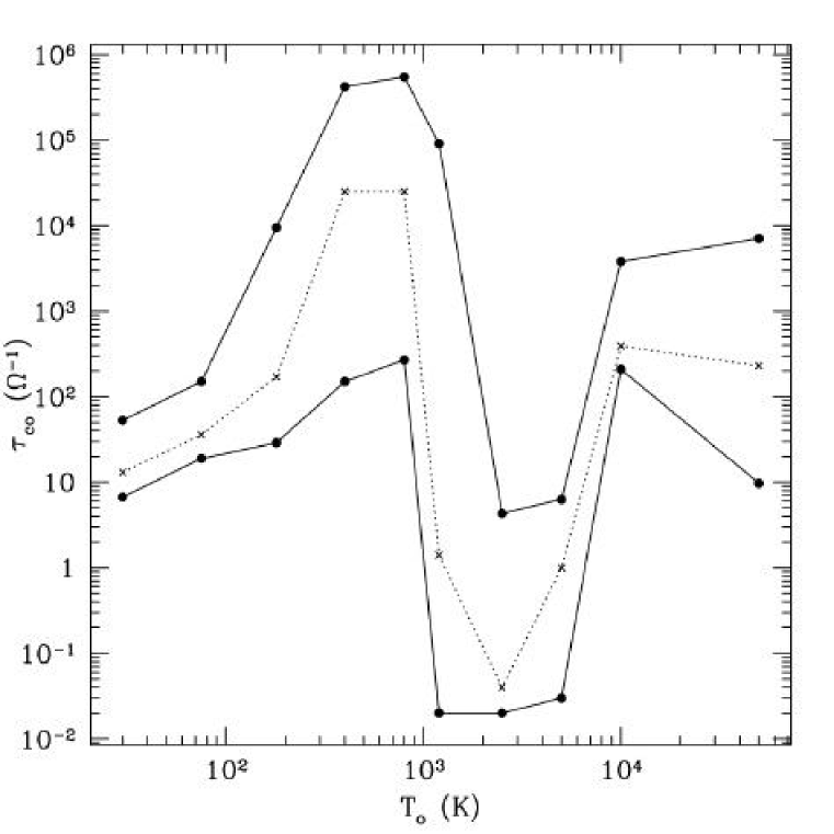
Figure 2.9: Initial cooling times at the points of non-fragmentation, fragmentation and transition.

The physical argument for fragmentation at short cooling times is as follows (e.g. Shlosman et al. 1990). Thermal energy is supplied to the disk via shocks. Strong shocks occur when dense clumps collide with one another; this occurs on a dynamical timescale $\sim\Omega^{-1}$. If the disk cools itself more rapidly then shock heating cannot match cooling and fragmentation results. This argument is apparently contradicted by Figure 2.9. The resolution lies in finding an appropriate definition of cooling time. The disk loses thermal energy on the effective cooling timescale

$${{\langle}{\langle}\tau_{c}{\rangle}{\rangle}}^{-1}\equiv\frac{{\langle}{\langle}\Lambda{\rangle}{\rangle}}{{\langle}{\langle}U{\rangle}{\rangle}}.$$ (2.23)

Figure 2.11 shows the run of ${{\langle}{\langle}\tau_{c}{\rangle}{\rangle}}$ at the fragmentation, transition, and non-fragmentation points. Evidently ${{\langle}{\langle}\tau_{c}{\rangle}{\rangle}}$ at transition lies between $\Omega^{-1}$ and $10\Omega^{-1}$. Figure 2.11 shows the run of ${\tau_{co}}$ and ${{\langle}{\langle}\tau_{c}{\rangle}{\rangle}}$ on the transition line. Just below the opacity gap they differ by as much as four orders of magnitude.

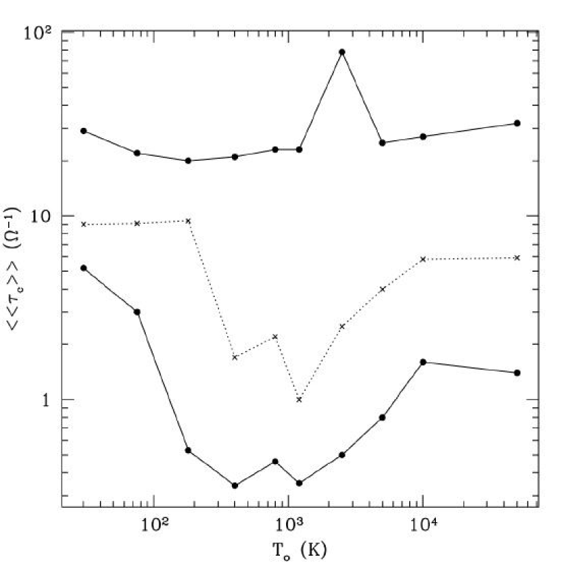
Figure 2.10: Effective cooling times at the points of non-fragmentation, fragmentation and transition.

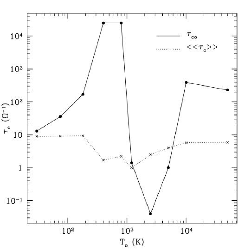
Figure 2.11: Initial and effective cooling times at the transition between non-fragmentation and fragmentation.

Why do ${\tau_{co}}$ and ${{\langle}{\langle}\tau_{c}{\rangle}{\rangle}}$ differ by such a large factor? The answer is related to the existence of sharp variations in opacity with temperature. Consider a disk near the lower edge of the opacity gap. Once gravitational instability sets in, fluctuations in temperature move parts of the disk into the opacity gap. There, the opacity is reduced by orders of magnitude. Since the cooling rate for an optically thick disk is proportional to $\kappa^{-1}$, the cooling time drops by a similar factor. Relatively small variations in temperature can thus produce large variations in cooling rate.

As in Gammie [2001], the result ${{\langle}{\langle}\tau_{c}{\rangle}{\rangle}}\Omega\gtrsim 1$ also implies a constraint on ${\langle}{\langle}\alpha{\rangle}{\rangle}$. Energy conservation implies that

$$\frac{3}{2}\Omega{\langle}{\langle}W_{xy}{\rangle}{\rangle}={\langle}{\langle}\Lambda{\rangle}{\rangle},$$ (2.24)

where $W_{xy}$ is the total shear stress (hydrodynamic plus gravitational). Equivalently, stress by rate-of-strain is equal to the dissipation rate. Using the definition of ${{\langle}{\langle}\tau_{c}{\rangle}{\rangle}}$, this implies

$${\langle}{\langle}\alpha{\rangle}{\rangle}=\left(\gamma(\gamma-1)\frac{9}{4}\Omega{{\langle}{\langle}\tau_{c}{\rangle}{\rangle}}\right)^{-1}.$$ (2.25)

Hence ${{\langle}{\langle}\tau_{c}{\rangle}{\rangle}}\Omega\gtrsim 1$ implies ${\langle}{\langle}\alpha{\rangle}{\rangle}\lesssim 1$. Figure 2.12 shows ${\langle}{\langle}\alpha{\rangle}{\rangle}$ vs ${{\langle}{\langle}\tau_{c}{\rangle}{\rangle}}$ for a large number of runs plotted against equation (2.25). For small values of ${{\langle}{\langle}\tau_{c}{\rangle}{\rangle}}$ the numerical values lie below the line. These models are not in equilibrium (i.e., not in a statistically-steady gravito-turbulent state), so the time average used in equation (2.24) is not well defined. For larger values of ${{\langle}{\langle}\tau_{c}{\rangle}{\rangle}}$ numerical results typically (there is noise in the measurement of both ${\langle}{\langle}\alpha{\rangle}{\rangle}$ and ${{\langle}{\langle}\tau_{c}{\rangle}{\rangle}}$ because the time average is taken over a finite time interval) lie slightly above the analytic result.

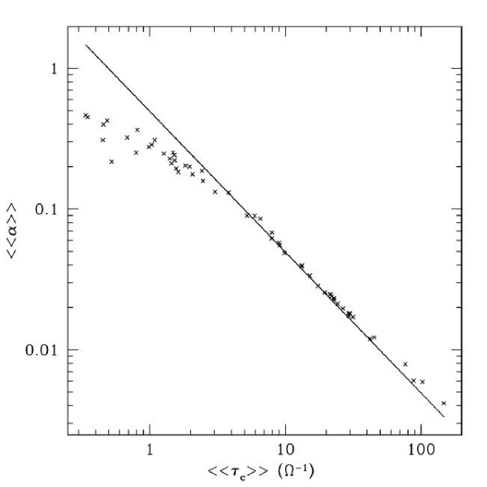
Figure 2.12: Time-averaged shear stress vs. effective cooling time for a series of runs. The solid line shows the analytic result, based on energy conservation, from equation (2.25).

The bias toward points lying slightly above the line reflects the fact that ${\langle}{\langle}\alpha{\rangle}{\rangle}$ measures the rate of energy extraction from the shear while ${{\langle}{\langle}\tau_{c}{\rangle}{\rangle}}$ measures the rate at which that energy is transformed into thermal energy. If energy is lost, perhaps to numerical averaging at the grid scale, then more energy must be extracted from the shear flow to make up the difference. Overall, however, the agreement with the analytic result is good and demonstrates good energy conservation in the code.

The relationship between ${{\langle}{\langle}\tau_{c}{\rangle}{\rangle}}$ and ${\langle}{\langle}\alpha{\rangle}{\rangle}$ is interesting but not particularly useful because ${{\langle}{\langle}\tau_{c}{\rangle}{\rangle}}$ is no more readily calculated than ${\langle}{\langle}\alpha{\rangle}{\rangle}$; it depends on a complicated moment of the surface density and temperature. Only for constant cooling time have we been able to evaluate this moment analytically.

2.5.3 Isothermal Disks

We have assumed that external illumination of the disk is negligible. This approximation is valid when the effective temperature $T_{irr}$ of the external irradiation is small compared to the central temperature of the disk. In the opposite limit, illumination controls the energetics of the disk and it is isothermal (if it is illuminated directly so that shadowing effects, such as those considered by Jang-Condell and Sasselov [2003] are negligible).

It is therefore worth studying the outcome of gravitational instability in an isothermal disk. The isothermal disk model has a single parameter: the initial value of $Q$. We ran models with varying values of $Q$ and with ${\langle}\delta v^{2}{\rangle}/c_{s}^{2}=0.1$. We find that models with $Q\lesssim 1.4$ fragment.

It is likely that the mass of the fragments, etc., depends on how an isothermal disk becomes unstable. Rapid fluctuation of the external radiation field is likely to produce a different outcome than dimming on a timescale long compared to the dynamical time.

2.6 Discussion

Using numerical experiments, we have identified those disks that are likely to fragment absent external heating. Disks with effective cooling times ${{\langle}{\langle}\tau_{c}{\rangle}{\rangle}}\lesssim\Omega^{-1}$ are susceptible to fragmentation. This is what one might expect based on the simple argument of Shlosman et al. [1990]: if the disk cools more quickly than the self-gravitating condensations can collide with one another, then those collisions (which occur on a timescale $\sim\Omega^{-1}$) cannot reheat the disk and fragmentation is inevitable. But our results are at the same time surprising.

The effective cooling time depends on the nonlinear outcome of gravitational instability. It depends on the cooling function, which in turn depends sensitively on $\Sigma$ and $U$. Since $\Sigma$ and $U$ vary strongly over the disk once gravitational instability has set in, it is difficult to estimate ${{\langle}{\langle}\tau_{c}{\rangle}{\rangle}}$ directly. One might be tempted to estimate ${{\langle}{\langle}\tau_{c}{\rangle}{\rangle}}(\Sigma,\Omega)\simeq{\tau_{co}}(\Sigma_{o},\Omega,Q=1)$, but our experiments show that this estimate can be off by as much as four orders of magnitude. The effect is particularly pronounced near sharp features in the opacity. For example, consider a model initially located just below the opacity gap with ${\tau_{co}}\Omega\gg 1$. Gravitational instability creates dense regions with higher temperatures, where dust is destroyed. The result is rather like having to shed one’s blanket on a cold winter morning: the disk loses its thermal energy suddenly. Pressure support is lost and gravitational collapse ensues.

The difference between ${{\langle}{\langle}\tau_{c}{\rangle}{\rangle}}$ and ${\tau_{co}}(Q=1)$ implies that a much larger region of the disk is susceptible to fragmentation than naive estimates based on the approximation ${{\langle}{\langle}\tau_{c}{\rangle}{\rangle}}\approx{\tau_{co}}$ might suggest. For example, consider an equilibrium disk model with $Q\gg 1$ at small $r$. As $r$ increases, $Q$ declines. Eventually $Q\sim 1$ and gravitational instability sets in. There is then a range of radii where $Q\sim 1$, ${{\langle}{\langle}\tau_{c}{\rangle}{\rangle}}\Omega\gtrsim 1$ and recurrent gravitational instability can transport angular momentum and prevent collapse. Generally speaking, however, the cooling time decreases with increasing radius. Eventually ${{\langle}{\langle}\tau_{c}{\rangle}{\rangle}}\Omega\sim 1$ and fragmentation cannot be avoided. By lowering our estimate of ${{\langle}{\langle}\tau_{c}{\rangle}{\rangle}}$, we narrow the range of radii over which recurrent gravitational instability can occur.

The general sense of our result is that it is extremely difficult to prevent a marginally-stable, $Q\sim 1$, optically-thick disk from fragmenting and forming planets (in circumstellar disks) or stars (in circumstellar and circumnuclear disks). This is particularly true for disks with $T\sim 10^{3}{\rm\,K}$, whose opacity is dominated by dust grains, i.e. disks whose temperature lies within a factor of several of the opacity gap.

Our numerical model uses a number of approximations. First, our treatment is razor-thin, i.e. all the matter is in a thin slice at $z=0$. The effect of finite thickness on linear stability has been understood since Goldreich and Lynden-Bell [1965]: it is stabilizing because gravitational attraction of neighboring columns of disk is diluted by finite thickness. The size of the effect may be judged by the fact that $Q=0.676$ is required for marginal stability of a finite-thickness, isothermal disk.

The behavior of a finite-thickness disk in the nonlinear regime is more difficult to predict. Shocks will evidently deposit some of their energy away from the midplane, where it can be radiated away more quickly (because the energy is deposited at smaller optical depth - see Pickett et al. 2000). Radiative diffusion parallel to the disk plane (not included here) may enhance cooling of dense, hot regions. Both these effects are destabilizing. Ultimately, however, a numerical study is required. This is numerically expensive: one must resolve the disk vertically, on the scale height $H$, and horizontally, at the critical wavelength $2\pi QH$.

Second, we have ignored magnetic fields. While there may be astrophysical situations where cool disks have such low ionization that they are unmagnetized, most disks are likely to contain dynamically important magnetic fields that give rise to a dimensionless shear stress ${\langle}{\langle}\alpha{\rangle}{\rangle}\gtrsim 0.01$ (e.g. Hawley et al. 1995). These fields are likely to remove spin angular momentum from partially collapsed objects, destabilizing them. Numerical experiments including both gravitational fields and magnetohydrodynamics are necessarily three dimensional (the instability of Balbus and Hawley [1991] requires $\partial_{z}\neq 0$), and are thus numerically expensive.

Third, we have fixed $\gamma$ and $\mu$ for the duration of each simulation. This eliminates the soft spots in the equation of state associated with ionization of atomic hydrogen and dissociation of molecular hydrogen. In these locations the three dimensional $\gamma$ dips below $4/3$, which is destabilizing.

Fourth, we have treated the physics of grain destruction and formation very simply. In using the Bell and Lin [1994] opacities we implicitly assume that grains reform in cooling gas on much less than a dynamical time. It is likely that grain re-formation will take some time (e.g. Hessman 1991) and this will further reduce the disk opacity and enhance fragmentation.

Fifth, we have neglected the effects of illumination. In the limit of strong external illumination, i.e. when the effective temperature of the irradiation $T_{irr}$ is large compared to the disk central temperature $T_{c}$, the disk is isothermal (here $T_{c}$ is the temperature of a dense condensation). We have carried out isothermal experiments and shown that, for initial velocity perturbations with ${\langle}\delta v^{2}{\rangle}/c_{s}^{2}=0.1$, disks with $Q\lesssim 1.4$ fragment. Weaker illumination produces a more complicated situation that we have not explored here. Illumination-dominated disks that become unstable presumably do so because the external illumination declines, and the rate at which the external illumination changes may govern the nonlinear outcome.

We conclude that disks with ${{\langle}{\langle}\tau_{c}{\rangle}{\rangle}}\Omega\lesssim 1$ do not exist. Cooling in this case is so effective that fragmentation into condensed objects– stars, planets, or smaller accretion disks– is inevitable.

As an example application of this result, consider the model for the nucleus of NGC 1068 recently proposed by Lodato and Bertin [2003]. Their model is an extended marginally-stable self-gravitating disk of the type investigated here and originally proposed by Goldreich and Lynden-Bell [1965] for galactic disks and Paczyński [1978] for accretion disks, although their disk is sufficiently massive that it modifies the rotation curve as well. Based on their Figure 3, at a typical radius of $0.5{\rm\,pc}$, $\Sigma_{o}\simeq 10^{4}$ and $\Omega\simeq 10^{-9}$. According to our Figure 7 this disk is about 2 orders of magnitude too dense to avoid fragmentation. While it may be possible to avoid this conclusion by invoking strong external heating, the energy requirements are severe, as outlined in Goodman [2003]. The disk proposed by Lodato and Bertin [2003] would therefore fragment into stars on a short timescale.

Chapter 3 Linear Theory of Thin, Radially-Stratified Disks

3.1 Chapter Overview

We consider the nonaxisymmetric linear theory of radially-stratified disks. We work in a shearing-sheet-like approximation, where the vertical structure of the disk is neglected, and develop equations for the evolution of a plane-wave perturbation comoving with the shear flow (a shearing wave, or “shwave”). We calculate a complete solution set for compressive and incompressive short-wavelength perturbations in both the stratified and unstratified shearing-sheet models. We develop expressions for the late-time asymptotic evolution of an individual shwave as well as for the expectation value of the energy for an ensemble of shwaves that are initially distributed isotropically in $k$-space. We find that: (i) incompressive, short-wavelength perturbations in the unstratified shearing sheet exhibit transient growth and asymptotic decay, but the energy of an ensemble of such shwaves is constant with time; (ii) short-wavelength compressive shwaves grow asymptotically in the unstratified shearing sheet, as does the energy of an ensemble of such shwaves; (iii) incompressive shwaves in the stratified shearing sheet have density and azimuthal velocity perturbations $\delta\Sigma$, $\delta v_{y}\sim t^{-{\rm Ri}}$ (for $|{\rm Ri}|\ll 1$), where ${\rm Ri}\equiv N_{x}^{2}/({\tilde{q}}\Omega)^{2}$ is the Richardson number, $N_{x}^{2}$ is the square of the radial Brunt-V$\ddot{\rm{a}}$is$\ddot{\rm{a}}$l$\ddot{\rm{a}}$ frequency and ${\tilde{q}}\Omega$ is the effective shear rate; (iv) the energy of an ensemble of incompressive shwaves in the stratified shearing sheet behaves asymptotically as ${\rm Ri}\,t^{1-4{\rm Ri}}$ for $|{\rm Ri}|\ll 1$. For Keplerian disks with modest radial gradients, $|{\rm Ri}|$ is expected to be $\ll 1$, and there will therefore be weak growth in a single shwave for ${\rm Ri}<0$ and near-linear growth in the energy of an ensemble of shwaves, independent of the sign of Ri.

3.2 Introduction

Angular momentum transport is central to the evolution of astrophysical disks. In many disks angular momentum is likely redistributed internally by magnetohydrodynamic (MHD) turbulence driven by the magnetorotational instability (MRI; see Balbus and Hawley 1998). But in portions of disks around young, low-mass stars, in cataclysmic-variable disks in quiescence, and in X-ray transients in quiescence [Stone et al., 2000, Gammie and Menou, 1998, Menou, 2000], disks may be composed of gas that is so neutral that the MRI fails. It is therefore of interest to understand if there are purely hydrodynamic mechanisms for driving turbulence and angular momentum transport in disks.

The case for hydrodynamic angular momentum transport is not promising. Numerical experiments carried out under conditions similar to those under which the MRI produces ample angular momentum fluxes– local shearing-box models– show small or negative angular momentum fluxes when the magnetic field is turned off [Hawley et al., 1995, 1996]. Unstratified shearing-sheet models show decaying angular momentum flux and kinetic energy when nonlinearly perturbed, yet recover the well known, high Reynolds number nonlinear instability of plane Couette flow when the parameters of the model are set appropriately (Balbus et al. 1996; see, however, the recent results by Umurhan and Regev 2004). Local models with unstable vertical stratification show overturning and the development of convective turbulence, but the mean angular momentum flux is small and of the wrong sign [Stone and Balbus, 1996].

Linear theory of global disk models has long indicated the presence of instabilities associated with reflecting boundaries or features in the flow (see e.g., Papaloizou and Pringle 1984, 1985, 1987, Goldreich et al. 1986, Goodman et al. 1987, Narayan et al. 1987, Lovelace et al. 1999, Li et al. 2000). Numerical simulations of the nonlinear outcome of these instabilities suggest that they saturate at low levels and are turned off by modest accretion [Blaes, 1987, Hawley, 1991]. One might guess that in the nonlinear outcome these instabilities will attempt to smooth out the features that give rise to them, much as convection tends to erase its parent entropy gradient. There are some suggestions, however, that such instabilities saturate into long-lived vortices, which may serve as obstructions in the flow that give rise to angular momentum transport [Li et al., 2001]. We will consider this possibility in a later publication.

Linear theory has yet to uncover a local instability of hydrodynamic disks that produces astrophysically-relevant angular momentum fluxes. Because of the absence of a complete set of modes in the shearing-sheet model, however, local linear stability is difficult to prove. Local nonlinear stability may be impossible to prove. Comparison with laboratory Couette flow experiments is complicated by several factors, not least of which is the inevitable presence of solid radial boundaries in the laboratory that have no analogue in astrophysical disks.

Recently, however, Klahr and Bodenheimer [2003] (hereafter KB03) have claimed to find a local hydrodynamic instability in global numerical simulations: the “Global Baroclinic Instability.” The instability arises in a model with scale-free initial conditions (an equilibrium entropy profile that varies as a power-law in radius) and thus does not depend on sharp features in the flow. Klahr [2004] has performed a local linear stability analysis of a radially-stratified accretion disk in an effort to explain the numerical results obtained by KB03. The instability mechanism invoked is the phenomenon of transient amplification as a shearing wave goes from leading to trailing. This is the mechanism that operates for nonaxisymmetric shearing waves in a disk that is nearly unstable to the axisymmetric gravitational instability [Goldreich and Lynden-Bell, 1965, Julian and Toomre, 1966, Goldreich and Tremaine, 1978]. It is the purpose of this work to clarify and extend the linear analysis of Klahr [2004]. If this instability exists it could be important for the evolution of low-ionization disks.

To isolate the cause for instabilities originally observed in global 3D simulations, KB03 perform both local and global 2D calculations in the ($R,\phi$)-plane. The local simulations use a new set of boundary conditions termed the shearing-disk boundary conditions. The model is designed to simulate a local portion of the disk without neglecting global effects such as curvature and horizontal flow gradients. The boundary conditions, which are described in more detail in KB03, require the assumption of a power-law scaling for the mean values of each of the variables, as well as the assumption that the fluctuations in each variable are proportional to their mean values. The radial velocity component in the inner and outer four grid cells is damped by $5\%$ each time step in order to remove artificial radial oscillations produced by the model.

The equilibrium profile for KB03’s 2D runs was a constant surface density $\Sigma$ with either a constant temperature $T$ or a temperature profile $T\propto R^{-1}$. The constant-$T$ runs showed no instability while those with varying $T$ (and thus varying entropy) sustained turbulence and positive Reynolds stresses. The fiducial local simulations were run at a resolution of $64^{2}$, with a spatial domain of $R=4$ to $6$ AU and $\Delta\phi=30\,^{\circ}$. The unstable run was repeated at a resolution of $128^{2}$, along with a run at twice the physical size of the fiducial runs. One global model (with nonreflecting outflow boundary conditions) was run at a resolution of $128^{2}$ with a spatial domain of $R=1$ to $10$ AU and $\Delta\phi=360\,^{\circ}$. All the runs yielded similar results, with the larger simulations producing vortices and power on large scales.

KB03 have chosen the term “baroclinic instability” by way of analogy with the baroclinic instability that gives rise to weather patterns in the atmosphere of the Earth and other planets (see e.g. Pedlosky 1979). The analogy is somewhat misleading, however, since the baroclinic instability that arises in planetary contexts is due to a baroclinic equilibrium. In a planetary atmosphere, a baroclinically-unstable situation requires stratification in both the vertical and latitudinal directions. The stratification in KB03 is only in the radial direction, and as a result the equilibrium is barotropic. It is the perturbations that are baroclinic; i.e., the disk is only baroclinic at linear order in the amplitude of a disturbance.

Cabot [1984] and Knobloch and Spruit [1986] have analyzed a thin disk with a baroclinic equilibrium state (with both vertical and radial gradients). The latter find that due to the dominant effect of the Keplerian shear, the instability only occurs if the radial scale height is comparable to the vertical scale height, a condition which is unlikely to be astrophysically relevant. As pointed out in KB03, the salient feature that is common to their analysis and the classical baroclinic instability is an equilibrium entropy gradient in the horizontal direction. As we show in §2, however, an entropy gradient is not required in order for two-dimensional perturbations to be baroclinic; any horizontal stratification will do.

The “Global Baroclinic Instability” claimed by KB03 is thus analogous to the classical baroclinic instability in the sense that both have the potential to give rise to convection. When neglecting vertical structure, however, the situation in an accretion disk is more closely analogous to a shearing, stratified atmosphere, the stability of which is governed by the classical Richardson criterion [Miles, 1961, Chimonas, 1970]. The only additional physics in a disk is the presence of the Coriolis force. Most analyses of a shearing, stratified atmosphere, however, only consider stratification profiles that are stable to convection. The primary question that Klahr [2004] and this work are addressing, then, is whether or not the presence of shear stabilizes a stratified equilibrium that would be unstable in its absence.

We begin in §3.3 by outlining the basic equations for a local model of a thin disk. §§3.4 and 3.5 describe the local linear theory for nonaxisymmetric sinusoidal perturbations in unstratified and radially-stratified disks, respectively. We summarize and discuss the implications of our findings in §3.6.

3.3 Basic Equations

The effect of radial gradients on the local stability of a thin disk can be analyzed most simply in the two-dimensional shearing-sheet approximation. This is obtained by a rigorous expansion of the equations of motion in the ratio of the vertical scale height $H$ to the local radius $R$, followed by a vertical integration of the fluid equations. The basic equations that one obtains (e.g., Goldreich and Tremaine 1978) are

$$\frac{d\Sigma}{dt}+\Sigma\mbox{\boldmath$\nabla$}\cdot\mbox{\boldmath$v$}=0,$$ (3.1)

$$\frac{d\mbox{\boldmath$v$}}{dt}+\frac{\mbox{\boldmath$\nabla$}P}{\Sigma}+2\mbox{\boldmath$\Omega$}\times\mbox{\boldmath$v$}-2q\Omega^{2}x\hat{\mbox{\boldmath$x$}}=0,$$ (3.2)

$$\frac{d\,{\rm{ln}}S}{dt}=0,$$ (3.3)

where $\Sigma$ and $P$ are the two-dimensional density and pressure, $S\equiv P\Sigma^{-\gamma}$ is monotonically related to the fluid entropy, $v$ is the fluid velocity and $d/dt$ is the Lagrangian derivative. The third and fourth terms in equation (3.2) represent the Coriolis and centrifugal forces in the local model expansion, where $\Omega$ is the local rotation frequency, $x$ is the radial Cartesian coordinate and $q$ is the shear parameter (equal to $1.5$ for a disk with a Keplerian rotation profile). The gravitational potential of the central object is included as part of the centrifugal force term in the local-model expansion, and we ignore the self-gravity of the disk.

It is worth emphasizing at this point that we have integrated out the vertical degrees of freedom in the model. We will later focus on perturbations with planar wavelengths that are small compared to a scale height, and these perturbations will be strongly influenced by the vertical structure of the disk.

Equations (3.1) through (3.3) can be combined into a single equation governing the evolution of the potential vorticity:

$$\frac{d}{dt}\left(\frac{\mbox{\boldmath$\nabla$}\times\mbox{\boldmath$v$}+2\mbox{\boldmath$\Omega$}}{\Sigma}\right)\equiv\frac{d\mbox{\boldmath$\xi$}}{dt}=\frac{\mbox{\boldmath$\nabla$}\Sigma\times\mbox{\boldmath$\nabla$}P}{\Sigma^{3}}.$$ (3.4)

In two dimensions, $\xi$ has only one nonzero component and can therefore be regarded as a scalar. Equation (3.4) demonstrates that for $P\equiv P(\Sigma)$ (as in the case of a strictly adiabatic evolution with isentropic initial conditions), the potential vorticity of fluid elements is conserved. For $P\neq P(\Sigma)$, however, the potential vorticity evolves with time. A barotropic equilibrium stratification can result in baroclinic perturbations that cause the potential vorticity to evolve at linear order. This can be seen by linearizing the scalar version of equation (3.4):

$$\frac{\partial\delta\xi}{\partial t}+\mbox{\boldmath$v$}_{0}\cdot\mbox{\boldmath$\nabla$}\delta\xi+\delta\mbox{\boldmath$v$}\cdot\mbox{\boldmath$\nabla$}\xi_{0}=\frac{\hat{\mbox{\boldmath$z$}}\cdot(\mbox{\boldmath$\nabla$}\Sigma_{0}\times\mbox{\boldmath$\nabla$}\delta P-\mbox{\boldmath$\nabla$}P_{0}\times\mbox{\boldmath$\nabla$}\delta\Sigma)}{\Sigma_{0}^{3}},$$ (3.5)

where we have dropped the term $\propto\mbox{\boldmath$\nabla$}\Sigma_{0}\times\mbox{\boldmath$\nabla$}P_{0}$. Notice that an entropy gradient is not required for the evolution of the perturbed potential vorticity. For $S_{0}=P_{0}\Sigma_{0}^{\gamma}=constant$, equation (3.5) reduces to

$$\frac{\partial\delta\xi}{\partial t}+\mbox{\boldmath$v$}_{0}\cdot\mbox{\boldmath$\nabla$}\delta\xi+\delta\mbox{\boldmath$v$}\cdot\mbox{\boldmath$\nabla$}\xi_{0}=\frac{\hat{\mbox{\boldmath$z$}}\cdot(\mbox{\boldmath$\nabla$}P_{0}\times\mbox{\boldmath$\nabla$}\delta S)}{\gamma\Sigma_{0}^{2}S_{0}}.$$ (3.6)

Potential vorticity is conserved only in the limit of zero stratification ($P_{0}=constant$) or adiabatic perturbations ($\delta S=0$).

3.4 Unstratified Shearing Sheet

Our goal is to understand the effects of radial stratification, but we begin by developing the linear theory of the standard (unstratified) shearing sheet, in which the equilibrium density and pressure are assumed to be spatially constant. This will serve to establish notation and method of analysis and to highlight the changes introduced by radial stratification in the next section.

Our analysis follows that of Goldreich and Tremaine [1978] except for our neglect of self-gravity. The equilibrium consists of a uniform sheet with $\Sigma=\Sigma_{0}=constant$, $P=P_{0}=constant$, and $\mbox{\boldmath$v$}_{0}=-q\Omega x\hat{\mbox{\boldmath$y$}}$. We consider nonaxisymmetric Eulerian perturbations about this equilibrium with space-time dependence $\delta(t){\rm exp}(ik_{x}(t)x+ik_{y}y)$, where

$$k_{x}(t)\equiv k_{x0}+q\Omega k_{y}t$$ (3.7)

(with $k_{x0}$ and $k_{y}>0$ constant) is required to allow for a spatial Fourier decomposition of the perturbation. We will refer to these perturbations as shearing waves, or with some trepidation, but more compactly, as “shwaves”.

3.4.1 Linearized Equations

To linear order in the perturbation amplitudes, the dynamical equations reduce to

$$\frac{\dot{\delta\Sigma}}{\Sigma_{0}}+ik_{x}\delta v_{x}+ik_{y}\delta v_{y}=0,$$ (3.8)

$$\dot{\delta v}_{x}-2\Omega\delta v_{y}+ik_{x}\frac{\delta P}{\Sigma_{0}}=0,$$ (3.9)

$$\dot{\delta v}_{y}+(2-q)\Omega\delta v_{x}+ik_{y}\frac{\delta P}{\Sigma_{0}}=0,$$ (3.10)

$$\frac{\dot{\delta P}}{\Sigma_{0}}+c_{s}^{2}(ik_{x}\delta v_{x}+ik_{y}\delta v_{y})=0,$$ (3.11)

where $c_{s}^{2}=\gamma P_{0}/\Sigma_{0}$ is the square of the equilibrium sound speed and an over-dot denotes a time derivative.

The above system of equations admits four linearly-independent solutions. Two of these are the nonvortical shwaves (solutions for which the perturbed potential vorticity is zero), which in the absence of self-gravity can be solved for exactly. The remaining two solutions are the vortical shwaves. When $k_{y}\rightarrow 0$ the latter reduce to the zero-frequency modes of the axisymmetric version of equations (3.8) through (3.11). One of these (the entropy mode) remains unchanged in nonaxisymmetry (in a frame comoving with the shear). There is thus only one nontrivial vortical shwave in the unstratified shearing sheet.

In the limit of tightly-wound shwaves ($|k_{x}|\gg k_{y}$), the nonvortical and vortical shwaves are compressive and incompressive, respectively. In the short-wavelength limit ($Hk_{y}\gg 1$, where $H\equiv c_{s}/\Omega$ is the vertical scale height), the compressive and incompressive solutions remain well separated at all times, but for $Hk_{y}\lesssim O(1)$ there is mixing between them near $k_{x}=0$ as an incompressive shwave shears from leading to trailing.[Chagelishvili et al., 1997, ; also Goodman 2005, private communication] With the understanding that the distinction between compressive shwaves and incompressive shwaves as separate solutions is not valid for all time when $Hk_{y}\lesssim O(1)$, we generally choose to employ these terms over the more general but less intuitive terms “nonvortical” and “vortical.”

Based upon the above considerations, it is convenient to study the vortical shwave in the short-wavelength, low-frequency ($\partial_{t}\ll c_{s}k_{y}$) limit. This is equivalent to working in the Boussinesq approximation, which in the unstratified shearing sheet amounts to assuming incompressible flow. In this limit, equation (3.8) is replaced with

$$k_{x}\delta v_{x}+k_{y}\delta v_{y}=0.$$ (3.12)

This demonstrates the incompressive nature of the vortical shwave in the short-wavelength limit.

3.4.2 Solutions

In the unstratified shearing sheet, equation (3.5) for the perturbed potential vorticity can be integrated to give:

$$\delta\xi_{u}=\frac{ik_{x}\delta v_{y}-ik_{y}\delta v_{x}}{\Sigma_{0}}-\xi_{0}\frac{\delta\Sigma}{\Sigma_{0}}=constant,$$ (3.13)

where $\xi_{0}=(2-q)\Omega/\Sigma_{0}$ is the equilibrium potential vorticity and we have employed the subscript $u$ to highlight the fact that the perturbed potential vorticity is only constant in the unstratified shearing sheet. To obtain the compressive-shwave solutions, we set the constant $\delta\xi_{u}$ to zero. Combining equations (3.10) and (3.13) with $\delta\xi_{u}=0$, one obtains an expression for $\delta v_{xc}$ in terms of $\delta v_{yc}$ and its derivative:

$$\delta v_{xc}=\frac{c_{s}^{2}k_{x}k_{y}\delta v_{yc}-\xi_{0}\Sigma_{0}\dot{\delta v}_{yc}}{\xi_{0}^{2}\Sigma_{0}^{2}+c_{s}^{2}k_{y}^{2}},$$ (3.14)

where the subscript $c$ indicates a compressive shwave. The associated density and pressure perturbations are

$$\delta\Sigma_{c}=\frac{\delta P_{c}}{c_{s}^{2}}=i\frac{\xi_{0}\Sigma_{0}k_{x}\delta v_{yc}+k_{y}\dot{\delta v}_{yc}}{\xi_{0}^{2}\Sigma_{0}^{2}+c_{s}^{2}k_{y}^{2}}$$ (3.15)

via equation (3.13). Reinserting equation (3.14) into equation (3.10), taking one time derivative and replacing $\dot{\delta P}$ via equation (3.11), we obtain the following remarkably simple equation:

$$\ddot{\delta v}_{yc}+\left(c_{s}^{2}k^{2}+\kappa^{2}\right)\delta v_{yc}=0,$$ (3.16)

where $k^{2}=k_{x}^{2}+k_{y}^{2}$ and $\kappa^{2}=(2-q)\Omega^{2}$ is the epicyclic frequency. Changing to the dimensionless dependent variable

$$T\equiv i\sqrt{\frac{2c_{s}k_{y}}{q\Omega}}\left(q\Omega t+\frac{k_{x0}}{k_{y}}\right)\equiv i\sqrt{\frac{2c_{s}k_{y}}{q\Omega}}\,\tau$$ (3.17)

and defining

$$C\equiv\frac{c_{s}^{2}k_{y}^{2}+\kappa^{2}}{2q\Omega c_{s}k_{y}},$$ (3.18)

the equation governing $\delta v_{yc}$ becomes

$$\frac{d^{2}\delta v_{yc}}{dT^{2}}+\left(\frac{1}{4}T^{2}-C\right)\delta v_{yc}=0.$$ (3.19)

This is the parabolic cylinder equation (e.g. Abramowitz and Stegun 1972), the solutions of which are parabolic cylinder functions. One representation of the general solution is

$$\delta v_{yc}=e^{-\frac{i}{2}T^{2}}\left[c_{1}\,M\left(\frac{1}{4}-\frac{i}{2}C,\frac{1}{2},\frac{i}{2}T^{2}\right)+c_{2}\,T\,M\left(\frac{3}{4}-\frac{i}{2}C,\frac{3}{2},\frac{i}{2}T^{2}\right)\right],$$ (3.20)

where $c_{1}$ and $c_{2}$ are constants of integration and $M$ is a confluent hypergeometric function. This completely specifies the compressive solutions for the unstratified shearing sheet, for any value of $k_{y}$.

Equation (3.19) has been analyzed in detail by Narayan et al. [1987]; their modal analysis yields the analogue of equation (3.19) in radial-position space rather than in the radial-wavenumber ($k_{x}=k_{y}\tau$) space that forms the natural basis for our shwave analysis. One way of seeing the correspondence between the modes and shwaves is to take the Fourier transform of the asymptotic form of the solution. Appropriate linear combinations of the solutions given in equation (3.20) have the following asymptotic time dependence for $\tau\gg 1$:

$$\delta v_{yc}\propto\sqrt{\frac{2}{T}}\exp\left(\pm\frac{i}{4}T^{2}\right)\propto\frac{1}{\sqrt{k_{x}}}\exp\left(\pm i\int c_{s}k_{x}\,dt\right).$$ (3.21)

The Fourier transform of the above expression, evaluated by the method of stationary phase for $Hk_{y}\gg 1$, yields

$$\delta v_{yc}(X)\propto\sqrt{\frac{2}{X}}\exp\left(\pm\frac{i}{4}X^{2}\right),$$ (3.22)

which is equivalent to the expressions given for the modes analyzed by Narayan et al. [1987], in which the dimensionless spatial variable (with zero frequency, so that corotation is at $x=0$) is defined as

$$X\equiv\sqrt{\frac{2q\Omega k_{y}}{c_{s}}}x.$$ (3.23)

To obtain the incompressive shwave, we use the condition of incompressibility (equation (3.12)) to write $\delta v_{y}$ in terms of $\delta v_{x}$, and then combine the dynamical equations (3.9) and (3.10) to eliminate $\delta P$. The incompressive shwave is given by:

$$\delta v_{xi}=\delta v_{xi0}\frac{k_{0}^{2}}{k^{2}},$$ (3.24)

$$\delta v_{yi}=-\frac{k_{x}}{k_{y}}\delta v_{xi},$$ (3.25)

$$\frac{\delta\Sigma_{i}}{\Sigma_{0}}=\frac{\delta P_{i}}{\gamma P_{0}}=\frac{1}{ic_{s}k_{y}}\left(\frac{k_{x}}{k_{y}}\frac{\dot{\delta v}_{xi}}{c_{s}}+2(q-1)\Omega\frac{\delta v_{xi}}{c_{s}}\right),$$ (3.26)

where the subscript $i$ indicates an incompressive shwave, $k_{0}^{2}=k_{x0}^{2}+k_{y}^{2}$ and $\delta v_{xi0}$ is the value of $\delta v_{xi}$ at $t=0$. This solution is uniformly valid for all time to leading order in $(Hk_{y})^{-1}\ll 1$.

3.4.3 Energetics of the Incompressive Shwaves

We define the kinetic energy in a single incompressive shwave as

$$E_{ki}\equiv\frac{1}{2}\Sigma_{0}(\delta v_{xi}^{2}+\delta v_{yi}^{2})=\frac{1}{2}\Sigma_{0}\delta v_{xi}^{2}\frac{k^{2}}{k_{y}^{2}}=\frac{1}{2}\Sigma_{0}\delta v_{xi0}^{2}\frac{k_{0}^{4}}{k_{y}^{2}k^{2}},$$ (3.27)

which peaks at $k_{x}=0$. This is not the only possible definition for the energy associated with a shear-flow disturbance; see Appendix A of Narayan et al. [1987] for a discussion of the subtleties involved in defining a perturbation energy in a differentially-rotating system. The energy defined above can simply be regarded as a convenient scalar measure of the shwave amplitude.

One can also define an amplification factor for an individual shwave,

$${\cal A}\equiv\frac{E_{ki}(k_{x}=0)}{E_{ki}(t=0)}=1+\frac{k_{x0}^{2}}{k_{y}^{2}},$$ (3.28)

which indicates that an arbitrary amount of transient amplification in kinetic energy can be obtained as one increases the amount of swing for a leading shwave ($k_{x0}\ll-k_{y}$). This is essentially the mechanism invoked by Chagelishvili et al. [2003], Umurhan and Regev [2004] and Afshordi et al. [2004] to argue for the onset of turbulence in unmagnetized Keplerian disks.

Because only a small subset of all Fourier components achieve large amplification (those with initial wavevector very nearly aligned with the radius vector), one must ask what amplification is achieved for an astrophysically relevant set of initial conditions containing a superposition of Fourier components. It is natural to draw such a set of Fourier components from a distribution that is isotropic, or nearly so, when $k_{0}$ is large.

Consider, then, perturbing a disk with a random set of incompressive perturbations (initial velocities perpendicular to $\mbox{\boldmath$k$}_{0}$) drawn from an isotropic, Gaussian random field and asking how the expectation value for the kinetic energy associated with the perturbations evolves with time. The evolution of the expected energy density is given by the following integral:

$${\langle}E_{i}{\rangle}=L^{2}\int d^{2}k_{0}{\langle}E_{ki}{\rangle}=L^{2}\int d^{2}k_{0}\frac{1}{2}\Sigma_{0}{\langle}\delta v_{xi0}^{2}{\rangle}\frac{k_{0}^{4}}{k_{y}^{2}k^{2}}.$$ (3.29)

where ${\langle}{\rangle}$ indicates an average over an ensemble of initial conditions, the first equality follows from Parseval’s theorem, the second equality follows from the incompressive shwave solution (3.24)-(3.26) and therefore applies only for $k_{0}H\gg 1$, and $L^{2}$ is a normalizing factor with units of length squared.

For initial conditions that are isotropic in $\mbox{\boldmath$k$}_{0}$ ($\delta v_{xi0}=\delta v_{\perp}(k_{0},\theta)\sin\theta$, where ${\langle}\delta v_{\perp}^{2}(k_{0}){\rangle}$ is the expectation value for the initial incompressive perturbation as a function of $k_{0}$ and $\tan\theta=k_{y}/k_{x0}$), the integral becomes

$${\langle}E_{i}{\rangle}=\frac{1}{2}\Sigma_{0}L^{2}\int k_{0}dk_{0}{\langle}\delta v_{\perp}^{2}(k_{0}){\rangle}\int_{0}^{2\pi}d\theta\,\frac{1}{\sin^{2}\theta+(q\Omega t\sin\theta+\cos\theta)^{2}}.$$ (3.30)

Changing integration variables to $\tau=q\Omega t+\cot\theta$, the angular integral becomes

$$\int_{-\infty}^{\infty}d\tau\,\frac{2}{1+\tau^{2}}=2\pi,$$ (3.31)

which is independent of time; hence

$${\langle}E_{i}{\rangle}={\langle}E_{i}(t=0){\rangle}$$ (3.32)

and we do not expect the total energy in incompressive shwaves to evolve. This same calculation has been performed in the context of plane Couette flow by Shepherd [1985], who also points out that the amplification factor due to a distribution of wavevectors in an angular wedge $\Delta\theta$ has an upper bound of $2\pi/(\Delta\theta)$. This indicates that the amplification will be modest unless the initial disturbance is narrowly concentrated around a single wavevector.

Although this result may appear to depend in detail on the assumption of isotropy, one can show that it really only depends on ${\langle}E_{ki}(t=0){\rangle}$ being smooth near $\sin\theta=0$, i.e. that there should not be a concentration of power in nearly radial wavevectors. This can be seen from the following argument. If we relax the assumption of isotropy, the angular integral becomes

$$\int_{0}^{2\pi}d\theta\,\frac{{\langle}\delta v_{\perp}^{2}(k_{0},\theta){\rangle}}{\sin^{2}\theta+(q\Omega t\sin\theta+\cos\theta)^{2}}.$$ (3.33)

For $q\Omega t\gg 1$ the above integrand is sharply peaked in the narrow regions around $\tan\theta=-1/(q\Omega t)\ll 1$ (i.e., $\sin\theta\simeq 0$). One can perform a Taylor-series expansion of ${\langle}\delta v_{\perp}^{2}(k_{0},\theta){\rangle}$ in these regions, and as long as ${\langle}\delta v_{\perp}^{2}(k_{0},\theta){\rangle}$ itself is not sharply peaked it is well approximated as a constant. A modest relaxation of the assumption of isotropy, then, will result in an asymptotically constant value for the energy integral.

Based upon this analysis, large amplification in an individual shwave does not in itself argue for a transition to turbulence due to transient growth. One must also demonstrate that a “natural” set of perturbations can extract energy from the background shear flow. In the case of the unstratified shearing sheet, the energy of a random set of incompressive perturbations remains constant with time. This is consistent with the results of Umurhan and Regev [2004], who see asymptotic decay in linear theory, because they work with a finite set of wavevectors, each of which must decay asymptotically.

3.4.4 Energetics of the Compressive Shwaves

Here we calculate the energy evolution of the compressive shwaves for comparison purposes. We will consider the evolution of short-wavelength compressive shwaves in which only the initial velocity is perturbed, both for simplicity and for consistency with our calculation of the short-wavelength incompressive shwaves. As before, we will assume that the initial kinetic energy is distributed isotropically.

We use the WKB solutions to equation (3.16) with $Hk_{y}\gg 1$. With the initial density perturbation set to zero (consistent with our assumption of only initial velocity perturbations), the uniformly-valid asymptotic solution to leading order in $(Hk_{y})^{-1}$ is given by

$$\delta v_{yc}=\delta v_{yc0}\sqrt{\frac{k_{0}}{k}}\cos(W-W_{0}),$$ (3.34)

$$\delta v_{xc}=\frac{k_{x}}{k_{y}}\delta v_{yc},$$ (3.35)

$$\delta\Sigma_{c}=\frac{i}{c_{s}^{2}k_{y}}\dot{\delta v}_{yc},$$ (3.36)

where the WKB eikonal is given by

$$W\equiv\int c_{s}k\,dt=\frac{Hk_{y}}{q}\int\sqrt{1+\tau^{2}}\,d\tau=\frac{Hk_{y}}{2q}\left(\tau\sqrt{1+\tau^{2}}+\ln\left(\tau+\sqrt{1+\tau^{2}}\right)\right),$$ (3.37)

with $W_{0}$ being the value of $W$ at $t=0$.

Using equation (3.35), the energy integral for the compressive shwaves in the short-wavelength limit is

$${\langle}E_{c}{\rangle}=L^{2}\int d^{2}k_{0}{\langle}E_{kc}{\rangle}=L^{2}\int d^{2}k_{0}\frac{1}{2}\Sigma_{0}{\langle}\delta v_{yc}^{2}{\rangle}\frac{k^{2}}{k_{y}^{2}}.$$ (3.38)

With initial velocities now parallel to ${\mbox{\boldmath$k$}}_{0}$ (and again isotropic), this becomes

$${\langle}E_{c}{\rangle}=\frac{1}{2}\Sigma_{0}L^{2}\int k_{0}dk_{0}{\langle}\delta v_{\|}^{2}(k_{0}){\rangle}\int_{0}^{2\pi}d\theta\,\sqrt{\sin^{2}\theta+(q\Omega t\sin\theta+\cos\theta)^{2}}\cos^{2}(W-W_{0}).$$ (3.39)

For $q\Omega t\gg 1$, the angular integral is approximated by

$$\int_{0}^{2\pi}d\theta\,|\sin\theta|\left(1+\cos(2W-2W_{0})\right)\simeq 2q\Omega t+\sqrt{\frac{2\pi q\Omega}{c_{s}k_{0}}}\cos(c_{s}k_{0}q\Omega t^{2}-\pi/4),$$ (3.40)

where the second approximation comes from employing the method of stationary phase. In the short-wavelength limit, then,

$${\langle}E_{c}(q\Omega t\gg 1){\rangle}=2q\Omega t\,{\langle}E_{c}(t=0){\rangle}.$$ (3.41)

Thus the kinetic energy of an initially isotropic distribution of compressive shwaves grows, presumably at the expense of the background shear flow.

The fate of a single compressive shwave is to steepen into a weak shock train and then decay. The fate of the field of weak shocks generated by an ensemble of compressive shwaves is less clear, but the mere presence of weak shocks does not indicate a transition to turbulence.

3.5 Radially-Stratified Shearing Sheet

We now generalize our analysis to include the possibility that the background density and pressure varies with $x$; this stratification is required for the manifestation of a convective instability. In order to use the shwave formalism we must assume that the background varies on a scale $L\sim H\ll R$ so that the local model expansion (e.g., the neglect of curvature terms in the equations of motion) is still valid.

With this assumption the equilibrium condition becomes

$$\mbox{\boldmath$v$}_{0}=\left(-q\Omega x+\frac{P_{0}^{\prime}(x)}{2\Omega\Sigma_{0}(x)}\right)\hat{\mbox{\boldmath$y$}},$$ (3.42)

where a prime denotes an $x$-derivative. One can regard the background flow as providing an effective shear rate

$${\tilde{q}}\Omega\equiv-v_{0}^{\prime}$$ (3.43)

that varies with $x$, in which case $\mbox{\boldmath$v$}_{0}=-\int^{x}{\tilde{q}}(s)ds\,\Omega\hat{\mbox{\boldmath$y$}}$.

Localized on this background flow we will consider a shearing wave with $k_{y}L\gg 1$. That is, we will consider nonaxisymmetric short-wavelength Eulerian perturbations with spacetime dependence $\delta(t)\exp(i\int^{x}\tilde{k}_{x}(t,s)ds+ik_{y}y+ik_{z}z)$, where $k_{y}$ and $k_{z}$ are constants and

$$\tilde{k}_{x}(t,x)\equiv k_{x0}+{\tilde{q}}(x)\Omega k_{y}t.$$ (3.44)

It may not be immediately obvious that this is a valid expansion since the shwaves sit on top of a radially-varying background (see Toomre 1969 for a discussion of waves in a slowly-varying background). But this is an ordinary WKB expansion in disguise. To see this, one need only transform to “comoving” coordinates $x^{\prime}=x$, $y^{\prime}=y+\int^{x}{\tilde{q}}(s)ds\Omega t$, $t^{\prime}=t$ (this procedure may be more familiar in a cosmological context; as Balbus [1988] has pointed out, this is possible for any flow in which the velocities depend linearly on the spatial coordinates). In this frame the time-dependent wavevector given above is transformed to a time-independent wavevector. The price paid for this is that $\partial_{x}\rightarrow\partial_{x^{\prime}}+{\tilde{q}}\Omega t\partial_{y^{\prime}}$, so new explicit time dependences appear on the right hand side of the perturbed equations of motion, and the perturbed variables no longer have time dependence $\exp(i\omega t^{\prime})$. Instead, we must solve an ODE for $\delta(t^{\prime})$. The $y^{\prime}$ dependence can be decomposed as $\exp(ik_{y}y^{\prime})$. The $x^{\prime}$ dependence can be treated via WKB, since the perturbation may be assumed to have the form $W(\epsilon x^{\prime},\epsilon t^{\prime})\,\exp(i\mbox{\boldmath$k$}^{\prime}\cdot\mbox{\boldmath$x$}^{\prime})$. This “nearly diagonalizes” the operator $\partial_{x^{\prime}}$. Thus we are considering the evolution of a wavepacket in comoving coordinates— a “shwavepacket”.

For this procedure to be valid two conditions must be met. First the usual WKB condition must apply, $k_{y}L\gg 1$. Second, the parameters of the flow that are “seen” by the shwavepacket must change little on the characteristic timescale for variation of $\delta(t)$, which is $\Omega^{-1}$ for the incompressive shwaves. For solid body rotation ($\tilde{q}=0$) the group velocity (derivable from equation [3.59], below) is $|v_{g}|<N_{x}/k$ (for positive squared Brunt-Väisälä frequency $N_{x}^{2}$, defined below; for $N_{x}^{2}<0$ the waves grow in place), so the timescale for change of wave packet parameters in this case is $L/|v_{g}|>kL/N_{x}\gg\Omega^{-1}$. It seems reasonable to anticipate similarly long timescales when shear is present. As a final check, we have verified directly, using a code based on the ZEUS code of Stone and Norman [1992], that a vortical shwavepacket in the stratified shearing sheet remains localized as it swings from leading to trailing.

3.5.1 Linearized Equations

To linear order in the perturbation amplitudes, the dynamical equations reduce to

$$\frac{\dot{\delta\Sigma}}{\Sigma_{0}}+\frac{\delta v_{x}}{L_{\Sigma}}+i\tilde{k}_{x}\delta v_{x}+ik_{y}\delta v_{y}+ik_{z}\delta v_{z}=0,$$ (3.45)

$$\dot{\delta v}_{x}-2\Omega\delta v_{y}+i\tilde{k}_{x}\frac{\delta P}{\Sigma_{0}}-\frac{c_{s}^{2}}{L_{P}}\frac{\delta\Sigma}{\Sigma_{0}}=0,$$ (3.46)

$$\dot{\delta v}_{y}+(2-{\tilde{q}})\Omega\delta v_{x}+ik_{y}\frac{\delta P}{\Sigma_{0}}=0,$$ (3.47)

$$\dot{\delta v}_{z}+ik_{z}\frac{\delta P}{\Sigma_{0}}=0,$$ (3.48)

$$\frac{\dot{\delta P}}{\Sigma_{0}}-c_{s}^{2}\frac{\dot{\delta\Sigma}}{\Sigma_{0}}+c_{s}^{2}\frac{\delta v_{x}}{L_{S}}=0,$$ (3.49)

where

$$\frac{1}{L_{P}}\equiv\frac{P_{0}^{\prime}}{\gamma P_{0}}=\frac{1}{L_{\Sigma}}+\frac{1}{L_{S}}\equiv\frac{\Sigma_{0}^{\prime}}{\Sigma_{0}}+\frac{S_{0}^{\prime}}{\gamma S_{0}}$$ (3.50)

define the equilibrium pressure, density and entropy length scales in the radial direction. We have included the vertical component of the velocity in order to make contact with an axisymmetric convective instability that is present in two dimensions, after which we will set $k_{z}$ to zero.

We will be mainly interested in the incompressive shwaves because the short-wavelength compressive shwaves are unchanged at leading order by stratification. We will therefore work solely in the Boussinesq approximation. In addition to the assumption of incompressibility, this approximation considers $\delta P$ to be negligible in the entropy equation; pressure changes are determined by whatever is required to maintain nearly incompressible flow. The original Boussinesq approximation applies only to incompressible fluids. It was extended to compressible fluids by Jeffreys [1930] and Spiegel and Veronis [1960]. We show in the Appendix that it is formally equivalent to taking the short-wavelength, low-frequency limit of the full set of linear equations. From this viewpoint, assuming that $Hk_{y}\delta P/P_{0}$ is of the same order as the other terms in the dynamical equations implies that $\delta P/P_{0}\sim(Hk_{y})^{-1}\delta\Sigma/\Sigma_{0}$, thus justifying its neglect in the entropy equation. We therefore replace equations (3.45) and (3.49) with

$$\tilde{k}_{x}\delta v_{x}+k_{y}\delta v_{y}+k_{z}\delta v_{z}=0$$ (3.51)

and

$$\frac{\dot{\delta\Sigma}}{\Sigma_{0}}-\frac{\delta v_{x}}{L_{S}}=0.$$ (3.52)

Using equations (3.47) and (3.52) and the time derivative of equation (3.51), one can express $\dot{\delta v}_{y}$ and $\delta P$ in terms of $\delta v_{x}$ and $\dot{\delta v}_{x}$:

$$\frac{\delta P}{\Sigma_{0}}=-i\frac{\tilde{k}_{x}\dot{\delta v}_{x}+2({\tilde{q}}-1)\Omega k_{y}\delta v_{x}}{k_{y}^{2}+k_{z}^{2}},$$ (3.53)

$$\dot{\delta v}_{y}=\frac{(-{\tilde{q}}k_{y}^{2}+({\tilde{q}}-2)k_{z}^{2})\Omega\delta v_{x}-\tilde{k}_{x}k_{y}\dot{\delta v}_{x}}{k_{y}^{2}+k_{z}^{2}}.$$ (3.54)

Eliminating $\delta P$ in equation (3.46) via equation (3.53) gives

$$\tilde{k}^{2}\dot{\delta v}_{x}+2({\tilde{q}}-1)\Omega\tilde{k}_{x}k_{y}\delta v_{x}=(k_{y}^{2}+k_{z}^{2})(2\Omega\delta v_{y}+(c_{s}^{2}/L_{P})\delta\Sigma/\Sigma_{0}),$$ (3.55)

where $\tilde{k}^{2}=\tilde{k}_{x}^{2}+k_{y}^{2}+k_{z}^{2}$. Taking the time derivative of this equation and eliminating $\dot{\delta\Sigma}$ and $\dot{\delta v}_{y}$ via equations (3.52) and (3.54), we obtain the following differential equation for $\delta v_{x}$:

$$\tilde{k}^{2}\ddot{\delta v}_{x}+4{\tilde{q}}\Omega\tilde{k}_{x}k_{y}\dot{\delta v}_{x}+\left[k_{y}^{2}\left(N_{x}^{2}+2{\tilde{q}}^{2}\Omega^{2}\right)+k_{z}^{2}\left(N_{x}^{2}+\tilde{\kappa}^{2}\right)\right]\delta v_{x}=0,$$ (3.56)

where $\tilde{\kappa}^{2}=2(2-{\tilde{q}})\Omega^{2}$ is the square of the effective epicyclic frequency and

$$N_{x}^{2}\equiv-\frac{c_{s}^{2}}{L_{S}L_{P}}$$ (3.57)

is the square of the Brunt-V$\ddot{\rm{a}}$is$\ddot{\rm{a}}$l$\ddot{\rm{a}}$ frequency in the radial direction.

3.5.2 Comparison with Known Results

Setting $k_{y}=0$ in equation (3.56) yields the axisymmetric modes with the following dispersion relation (for $\delta(t)\propto e^{-i\omega t}$):

$$\omega^{2}=\frac{k_{z}^{2}}{k_{x0}^{2}+k_{z}^{2}}\left(N_{x}^{2}+\tilde{\kappa}^{2}\right).$$ (3.58)

This is the origin of the Høiland stability criterion: the axisymmetric modes are stable for $N_{x}^{2}+\tilde{\kappa}^{2}>0$. In the absence of rotation this reduces to the Schwarzschild stability criterion: $N_{x}^{2}>0$ is the necessary condition for stability. The effect of rotation is strongly stabilizing: if $N_{x}^{2}<-\tilde{\kappa}^{2}$, as required for instability, then $L_{S}L_{P}\sim H^{2}$; pressure and entropy must vary on radial scales of order the scale height for the disk to be Høiland unstable.

Notice that effective epicyclic frequency $\tilde{\kappa}^{2}$ only stabilizes modes with nonzero $k_{z}$. The stability of nonaxisymmetric shwaves with $k_{z}=0$ (as in the mid-plane of a thin disk) is the open question that this work is addressing. In this limit and in the absence of shear the Schwarzschild stability criterion is again recovered: with $k_{z}=0$ and ${\tilde{q}}=0$ in equation (3.56) the dispersion relation becomes

$$\omega^{2}=\frac{k_{y}^{2}}{k_{x0}^{2}+k_{y}^{2}}N_{x}^{2},$$ (3.59)

If there is a region of the disk where the effective shear is zero, a WKB normal-mode analysis will yield the above dispersion relation and there will be convective instability for $N_{x}^{2}<0$. It appears from equation (3.56) that differential rotation provides a stabilizing influence for nonaxisymmetric shwaves just as rotation does for the axisymmetric modes. Things are not as simple in nonaxisymmetry, however. The time dependence is no longer exponential, nor is it the same for all the perturbation variables. There is no clear cutoff between exponential and oscillatory behavior, so the question of flow stability becomes more subtle.

As discussed in the introduction, the Boussinesq system of equations in the shearing-sheet model of a radially-stratified disk bear a close resemblance to the system of equations employed in analyses of a shearing, stratified atmosphere. A sufficient condition for stability in the latter case is that

$${\rm Ri}\equiv\frac{N_{x}^{2}}{(v_{0}^{\prime})^{2}}\geq\frac{1}{4}$$ (3.60)

everywhere in the flow, where Ri is the Richardson number, a measure of the relative importance of buoyancy and shear. This stability criterion was originally proved by Miles [1961] and Howard [1961] for incompressible fluids, and its extension to compressible fluids was demonstrated by Chimonas [1970]. The stability criterion is based on a normal-mode analysis with rigid boundary conditions. Other than differences in notation (e.g., our radial coordinate corresponds to the vertical coordinate in a stratified atmosphere), the key differences in our system are: (i) the equilibrium pressure gradient in a disk is balanced by centrifugal forces rather than by gravity; (ii) the disk equations contain Coriolis force terms; (iii) most atmospheric analyses only consider an equilibrium that is convectively stable, whereas we are interested in an unstable stratification; (iv) we do not employ boundary conditions in our analytic model since we are only interested in the possibility of a local instability.

The lack of boundary conditions in our model makes the applicability of the standard Richardson stability criterion in determining local stability somewhat dubious, since the lack of boundary conditions precludes the decomposition of linear disturbances into normal modes. The natural procedure for performing a local linear analysis in disks is to decompose the perturbations into shwaves, as we have done.

Eliassen et al. [1953] consider both stable and unstable atmospheres and analyze an initial-value problem by decomposing the perturbations in time via Laplace transforms. For flow between two parallel walls, they find that an arbitrary initial disturbance behaves asymptotically as $t^{(\alpha-1)/2}$ for $-3/4<{\rm Ri}<1/4$, where

$$\alpha\equiv\sqrt{1-4\,{\rm{Ri}}},$$ (3.61)

which grows algebraically for ${\rm Ri}<0$. The disturbance grows exponentially only for ${\rm Ri}<-3/4$. For a semi-infinite flow, the power-law behavior in time holds for $-2<{\rm Ri}<1/4$, with exponential growth for ${\rm Ri}<-2$. These results illustrate the importance of boundary conditions in determining stability.

In the $k_{z}=0$ limit that we are concerned with here, the correspondence between the disk and atmospheric models turns out to be exact in the shwave formalism. This is because the Coriolis force only appears in equation (3.56) via $\tilde{\kappa}^{2}$, which disappears when $k_{z}=0$. The equation describing the time evolution of shwaves in both a radially-stratified disk and a shearing, stratified atmosphere is thus

$$\tilde{k}^{2}\ddot{\delta v}_{x}+4{\tilde{q}}\Omega\tilde{k}_{x}k_{y}\dot{\delta v}_{x}+k_{y}^{2}\left(N_{x}^{2}+2{\tilde{q}}^{2}\Omega^{2}\right)\delta v_{x}=0.$$ (3.62)

We analyze the solutions to this equation in the following section.

3.5.3 Solutions

Changing time variables in equation (3.62) to $\tilde{\tau}\equiv\tilde{k}_{x}/k_{y}$, the differential equation governing $\delta v_{x}$ becomes

$$(1+\tilde{\tau}^{2})\frac{d^{2}\delta v_{x}}{d\tilde{\tau}^{2}}+4\tilde{\tau}\frac{d\delta v_{x}}{d\tilde{\tau}}+({\rm{Ri}}+2)\delta v_{x}=0.$$ (3.63)

The solutions to equation (3.63) are hypergeometric functions. With the change of variables $z\equiv-\tilde{\tau}^{2}$, equation (3.63) becomes

$$z(1-z)\frac{d^{2}\delta v_{x}}{dz^{2}}+\frac{1-5z}{2}\frac{d\delta v_{x}}{dz}-\frac{{\rm{Ri}}+2}{4}\delta v_{x}=0.$$ (3.64)

The hypergeometric equation [Abramowitz and Stegun, 1972]

$$z(1-z)\frac{d^{2}\delta v_{x}}{dz^{2}}+\left[c-(a+b+1)z\right]\frac{d\delta v_{x}}{dz}-ab\delta v_{x}=0$$ (3.65)

has as its two linearly independent solutions $F(a,b;c;z)$ and $z^{1-c}F(a-c+1,b-c+1;2-c;z)$. Comparison of equations (3.64) and (3.65) shows that $a=(3-\alpha)/4$, $b=(3+\alpha)/4$ and $c=1/2$, where $\alpha$ is defined in equation (3.61).

The general solution for $\delta v_{x}$ is thus given by

$$\delta v_{x}=C_{1}\,F\left(\frac{3-\alpha}{4},\frac{3+\alpha}{4};\frac{1}{2};-\tilde{\tau}^{2}\right)+C_{2}\,\tilde{\tau}\,F\left(\frac{5-\alpha}{4},\frac{5+\alpha}{4};\frac{3}{2};-\tilde{\tau}^{2}\right),$$ (3.66)

where $C_{1}$ and $C_{2}$ are constants of integration representing the two degrees of freedom in our reduced system. These two degrees of freedom can be represented physically by the initial velocity and displacement of a perturbed fluid particle in the radial direction. The radial Lagrangian displacement $\xi_{x}$ is obtained from equation (3.66) by direct integration,

$$\xi_{x}=\int\delta v_{x}\,dt=-\frac{C_{2}}{{\tilde{q}}\Omega{\rm Ri}}\,F\left(\frac{1-\alpha}{4},\frac{1+\alpha}{4};\frac{1}{2};-\tilde{\tau}^{2}\right)+\frac{C_{1}}{{\tilde{q}}\Omega}\,\tilde{\tau}\,F\left(\frac{3-\alpha}{4},\frac{3+\alpha}{4};\frac{3}{2};-\tilde{\tau}^{2}\right).$$ (3.67)

The solutions for the other perturbation variables can be obtained from equations (3.51), (3.52) and (3.53) with $k_{z}=0$:

$$\delta v_{y}=-\tilde{\tau}\delta v_{x},$$ (3.68)

$$\frac{\delta\Sigma}{\Sigma_{0}}=\frac{\xi_{x}}{L_{S}}$$ (3.69)

and

$$\frac{\delta P}{P_{0}}=\frac{\gamma\Omega}{ic_{s}k_{y}}\left[{\tilde{q}}\tilde{\tau}\frac{d}{d\tilde{\tau}}\left(\frac{\delta v_{x}}{c_{s}}\right)+2({\tilde{q}}-1)\frac{\delta v_{x}}{c_{s}}\right].$$ (3.70)

It can be seen from the latter equation and the solution for $\delta v_{x}$ that $\delta P/P_{0}$ remains small compared to $\delta v_{x}/c_{s}$ in the short-wavelength limit. This demonstrates the consistency of the Boussinesq approximation.

The hypergeometric functions can be transformed to a form valid for large $\tilde{\tau}$ (see Abramowitz and Stegun 1972 equations 15.3.7 and 15.1.1). An equivalent form of the solution for $|\tilde{\tau}|\gg 1$ is

$$\delta v_{x}=(C_{1}V_{1}+{\rm{sgn}}(\tilde{\tau})C_{2}V_{2})\,|\tilde{\tau}|^{\frac{\alpha-3}{2}}F\left(\frac{3-\alpha}{4},\frac{5-\alpha}{4};1-\frac{\alpha}{2};-\frac{1}{\tilde{\tau}^{2}}\right)+$$

$$(C_{1}V_{3}+{\rm{sgn}}(\tilde{\tau})C_{2}V_{4})\,|\tilde{\tau}|^{-\frac{\alpha+3}{2}}F\left(\frac{3+\alpha}{4},\frac{5+\alpha}{4};1+\frac{\alpha}{2};-\frac{1}{\tilde{\tau}^{2}}\right),\;\;\;$$ (3.71)

where ${\rm{sgn}}(\tilde{\tau})$ is the arithmetic sign of $\tilde{\tau}$ and the constants $V_{i}$ are given by

$$V_{1}\equiv\frac{\Gamma\left(\frac{1}{2}\right)\Gamma\left(\frac{\alpha}{2}\right)}{\Gamma\left(\frac{3+\alpha}{4}\right)\Gamma\left(-\frac{1-\alpha}{4}\right)}\;\;,\;\;V_{2}\equiv\frac{\Gamma\left(\frac{3}{2}\right)\Gamma\left(\frac{\alpha}{2}\right)}{\Gamma\left(\frac{5+\alpha}{4}\right)\Gamma\left(\frac{1+\alpha}{4}\right)},\;\;$$

$$V_{3}\equiv\frac{\Gamma\left(\frac{1}{2}\right)\Gamma\left(-\frac{\alpha}{2}\right)}{\Gamma\left(\frac{3-\alpha}{4}\right)\Gamma\left(-\frac{1+\alpha}{4}\right)}\;\;,\;\;V_{4}\equiv\frac{\Gamma\left(\frac{3}{2}\right)\Gamma\left(-\frac{\alpha}{2}\right)}{\Gamma\left(\frac{5-\alpha}{4}\right)\Gamma\left(\frac{1-\alpha}{4}\right)}.$$ (3.72)

Expanding the above form of the solution for $|\tilde{\tau}|\gg 1$, we obtain

$$\delta v_{x}=\left(C_{1}V_{1}+{\rm{sgn}}(\tilde{\tau})C_{2}V_{2}\right)\,|\tilde{\tau}|^{\frac{\alpha-3}{2}}+\left(C_{1}V_{3}+{\rm{sgn}}(\tilde{\tau})C_{2}V_{4}\right)\,|\tilde{\tau}|^{-\frac{\alpha+3}{2}}+O(\tilde{\tau}^{-2}).$$ (3.73)

An equivalent form of $\xi_{x}$ for $|\tilde{\tau}|\gg 1$ is

$$\xi_{x}=\left(-\frac{C_{2}X_{1}}{{\tilde{q}}\Omega{\rm Ri}}+{\rm{sgn}}(\tilde{\tau})\frac{C_{1}X_{2}}{{\tilde{q}}\Omega}\right)\,|\tilde{\tau}|^{\frac{\alpha-1}{2}}F\left(\frac{3-\alpha}{4},\frac{1-\alpha}{4};1-\frac{\alpha}{2};-\frac{1}{\tilde{\tau}^{2}}\right)+$$

$$\left(-\frac{C_{2}X_{3}}{{\tilde{q}}\Omega{\rm Ri}}+{\rm{sgn}}(\tilde{\tau})\frac{C_{1}X_{4}}{{\tilde{q}}\Omega}\right)\,|\tilde{\tau}|^{-\frac{\alpha+1}{2}}F\left(\frac{3+\alpha}{4},\frac{1+\alpha}{4};1+\frac{\alpha}{2};-\frac{1}{\tilde{\tau}^{2}}\right),\;\;\;$$ (3.74)

where the constants $X_{i}$ are given by

$$X_{1}\equiv\frac{\Gamma\left(\frac{1}{2}\right)\Gamma\left(\frac{\alpha}{2}\right)}{\Gamma\left(\frac{1+\alpha}{4}\right)\Gamma\left(\frac{1+\alpha}{4}\right)}\;\;,\;\;X_{2}\equiv\frac{\Gamma\left(\frac{3}{2}\right)\Gamma\left(\frac{\alpha}{2}\right)}{\Gamma\left(\frac{3+\alpha}{4}\right)\Gamma\left(\frac{3+\alpha}{4}\right)},\;\;$$

$$X_{3}\equiv\frac{\Gamma\left(\frac{1}{2}\right)\Gamma\left(-\frac{\alpha}{2}\right)}{\Gamma\left(\frac{1-\alpha}{4}\right)\Gamma\left(\frac{1-\alpha}{4}\right)}\;\;,\;\;X_{4}\equiv\frac{\Gamma\left(\frac{3}{2}\right)\Gamma\left(-\frac{\alpha}{2}\right)}{\Gamma\left(\frac{3-\alpha}{4}\right)\Gamma\left(\frac{3-\alpha}{4}\right)}.$$ (3.75)

Expanding $\xi_{x}$ for $|\tilde{\tau}|\gg 1$ yields

$$\xi_{x}=\left(-\frac{C_{2}X_{1}}{{\tilde{q}}\Omega{\rm Ri}}+{\rm{sgn}}(\tilde{\tau})\frac{C_{1}X_{2}}{{\tilde{q}}\Omega}\right)\,|\tilde{\tau}|^{\frac{\alpha-1}{2}}+\left(-\frac{C_{2}X_{3}}{{\tilde{q}}\Omega{\rm Ri}}+{\rm{sgn}}(\tilde{\tau})\frac{C_{1}X_{4}}{{\tilde{q}}\Omega}\right)\,|\tilde{\tau}|^{-\frac{\alpha+1}{2}}+O(\tilde{\tau}^{-2}).$$ (3.76)

The dominant contribution for each perturbation variable at late times is thus

$$\delta P\propto\delta v_{x}\sim t^{\frac{\alpha-3}{2}},$$ (3.77)

$$\delta\Sigma\propto\xi_{x}\sim t^{\frac{\alpha-1}{2}},$$ (3.78)

and

$$\delta v_{y}\propto t\delta v_{x}\sim t^{\frac{\alpha-1}{2}}.$$ (3.79)

This leads to one of our main conclusions: the density and $y$-velocity perturbations will grow asymptotically for $\alpha>1$, i.e. ${\rm{Ri}}\propto N_{x}^{2}<0$. For small Richardson number, however (as is expected for a Keplerian disk with modest radial gradients), $\alpha\sim 1-2{\rm Ri}$ and the asymptotic growth is extremely slow:

$$\delta\Sigma\sim\delta v_{y}\sim t^{-{\rm Ri}}.$$ (3.80)

In the stratified shearing sheet, the right-hand side of equation (3.5) governing the evolution of the perturbed potential vorticity is no longer zero. The form of this equation for the incompressive shwaves is

$$\dot{\delta\xi}=\frac{d}{dt}\left(\frac{i\tilde{k}_{x}\delta v_{y}-ik_{y}\delta v_{x}}{\Sigma_{0}}\right)=\frac{c_{s}^{2}k_{y}}{iL_{P}\Sigma_{0}^{2}}\delta\Sigma.$$ (3.81)

The asymptotic time dependence of the perturbed potential vorticity can be obtained by integrating equation (3.81):

$$\delta\xi\sim t^{\frac{\alpha+1}{2}}\sim t^{1-{\rm Ri}}$$ (3.82)

for $\tilde{\tau}\gg 1$ and $|{\rm Ri}|\ll 1$. As noted in §2, an entropy gradient is not required to generate vorticity. For $N_{x}^{2}=0$, $\alpha=1$ and the perturbed potential vorticity grows linearly with time. The unstratified shearing sheet is recovered in the limit of zero stratification ($1/L_{P}\rightarrow 0$), since in this limit equation (3.81) reduces to $\xi=constant$.

3.5.4 Energetics of the Incompressive Shwaves

For a physical interpretation of the incompressive shwaves in the stratified shearing sheet, we repeat the analysis of section 3.3 for the solution given in the previous section. For a complete description of the energy in this case, however, we must include the potential energy of a fluid element displaced in the radial direction. Following Miles [1961], an expression for the energy in the Boussinesq approximation is obtained by summing equation (3.46) multiplied by $\delta v_{x}$ and equation (3.47) multiplied by $\delta v_{y}$. Replacing $\delta\Sigma/\Sigma_{0}$ by $\xi_{x}/L_{S}$ via equation (3.69) results in the following expression for the energy evolution:

$$\frac{dE_{k}}{d\tilde{\tau}}\equiv\frac{d}{d\tilde{\tau}}\left(\frac{1}{2}\Sigma_{0}\delta v^{2}+\frac{1}{2}\Sigma_{0}N_{x}^{2}\xi_{x}^{2}\right)=\Sigma_{0}\delta v_{x}\delta v_{y},$$ (3.83)

where $\delta v^{2}=\delta v_{x}^{2}+\delta v_{y}^{2}$. The three terms in equation (3.83) can be identified as the kinetic energy, potential energy and Reynolds stress associated with an individual shwave. One may readily verify that the vortical shwaves (see equations (3.24)-(3.26)) in the unstratified shearing sheet ($N_{x}^{2}=0$) satisfy equation (3.83).

The right hand side of equation (3.83) can be rewritten $-\tilde{\tau}\delta v_{x}^{2}$ and individual trailing shwaves ($\tilde{\tau}>0$) are therefore associated with a negative angular momentum flux. If the energy were positive definite this would require that individual shwaves always decay. But when $N_{x}^{2}<0$ (${\rm Ri}<0$) the potential energy associated with a displacement is negative, so the energy $E_{k}$ can be negative and a negative angular momentum flux is not enough to halt shwave growth.

Our next step is to write the constants of integration $C_{1}$ and $C_{2}$ in terms of the initial radial velocity and displacement of the shearing wave, $\delta v_{x0}$ and $\xi_{x0}$:

$$C_{1}=\frac{{\tilde{q}}\Omega{\rm Ri}\,\delta v_{x2}(\tilde{\tau}_{0})\,\xi_{x0}+\xi_{x1}(\tilde{\tau}_{0})\,\delta v_{x0}}{\delta v_{x1}(\tilde{\tau}_{0})\,\xi_{x1}(\tilde{\tau}_{0})+{\rm Ri}\,\delta v_{x2}(\tilde{\tau}_{0})\,\xi_{x2}(\tilde{\tau}_{0})}\;\;,\;\;C_{2}=\frac{-{\tilde{q}}\Omega{\rm Ri}\,\delta v_{x1}(\tilde{\tau}_{0})\,\xi_{x0}+{\rm Ri}\,\xi_{x2}(\tilde{\tau}_{0})\,\delta v_{x0}}{\delta v_{x1}(\tilde{\tau}_{0})\,\xi_{x1}(\tilde{\tau}_{0})+{\rm Ri}\,\delta v_{x2}(\tilde{\tau}_{0})\,\xi_{x2}(\tilde{\tau}_{0})},$$ (3.84)

where $\tilde{\tau}_{0}=k_{x0}/k_{y}$, $\delta v_{x1}$ is the hypergeometric function given by equation (3.66) with $C_{1}=1$ and $C_{2}=0$, and the other functions are similarly defined. These expressions can be simplified by noticing that the denominator of $C_{1}$ and $C_{2}$ is the Wronskian of the differential equation for $\xi_{x}$:

$$(1+\tilde{\tau}^{2})\frac{d^{2}\xi_{x}}{d\tilde{\tau}^{2}}+2\tilde{\tau}\frac{d\xi_{x}}{d\tilde{\tau}}+{\rm Ri}\xi_{x}=0.$$ (3.85)

The Wronskian of this equation is

$${\cal W}\equiv\frac{d\xi_{x2}}{d\tilde{\tau}}\,\xi_{x1}-\frac{d\xi_{x1}}{d\tilde{\tau}}\,\xi_{x2}=\exp\left(-\int^{\tilde{\tau}}\frac{2\tau^{2}}{1+\tau^{2}}\,d\tau\right)=\frac{1}{1+\tilde{\tau}^{2}}.$$ (3.86)

We further simplify the analysis by setting the initial displacement $\xi_{x0}$ to zero.

With these simplifications, the solution given by equations (3.66) and (3.67) becomes

$$\frac{\delta v_{x}}{\delta v_{x0}}=\left(1+\tilde{\tau}_{0}^{2}\right)\left[F\left(\frac{1-\alpha}{4},\frac{1+\alpha}{4};\frac{1}{2};-\tilde{\tau}_{0}^{2}\right)\,F\left(\frac{3-\alpha}{4},\frac{3+\alpha}{4};\frac{1}{2};-\tilde{\tau}^{2}\right)+\right.$$

$$\left.{\rm Ri}\,\tilde{\tau}_{0}\,F\left(\frac{3-\alpha}{4},\frac{3+\alpha}{4};\frac{3}{2};-\tilde{\tau}_{0}^{2}\right)\,\tilde{\tau}\,F\left(\frac{5-\alpha}{4},\frac{5+\alpha}{4};\frac{3}{2};-\tilde{\tau}^{2}\right)\right],$$ (3.87)

$$\frac{\xi_{x}}{\delta v_{x0}}=\left(1+\tilde{\tau}_{0}^{2}\right)\left[-\frac{1}{{\tilde{q}}\Omega}\tilde{\tau}_{0}\,F\left(\frac{3-\alpha}{4},\frac{3+\alpha}{4};\frac{3}{2};-\tilde{\tau}_{0}^{2}\right)\,F\left(\frac{1-\alpha}{4},\frac{1+\alpha}{4};\frac{1}{2};-\tilde{\tau}^{2}\right)+\right.$$

$$\left.\frac{1}{{\tilde{q}}\Omega}F\left(\frac{1-\alpha}{4},\frac{1+\alpha}{4};\frac{1}{2};-\tilde{\tau}_{0}^{2}\right)\,\tilde{\tau}\,F\left(\frac{3-\alpha}{4},\frac{3+\alpha}{4};\frac{3}{2};-\tilde{\tau}^{2}\right)\right].$$ (3.88)

As in section 3.3, the energy integral for the incompressive perturbations is given by

$${\langle}E_{i}{\rangle}=\frac{1}{2}\Sigma_{0}L^{2}\int k_{0}dk_{0}{\langle}\delta v_{\perp}^{2}(k_{0}){\rangle}\int_{0}^{2\pi}d\theta\sin^{2}\theta\left[\left(1+\tilde{\tau}^{2}\right)\left(\frac{\delta v_{x}}{\delta v_{x0}}\right)^{2}+N_{x}^{2}\left(\frac{\xi_{x}}{\delta v_{x0}}\right)^{2}\right],$$ (3.89)

for initial perturbations perpendicular to and isotropic in $\mbox{\boldmath$k$}_{0}$. Changing integration variables to $\tilde{\tau}={\tilde{q}}\Omega t+\cot\theta$, the angular integral becomes

$$2\int_{-\infty}^{\infty}d\tilde{\tau}\,\left[\left(1+\tilde{\tau}^{2}\right)\left\{\xi_{x1}(\tilde{\tau}-{\tilde{q}}\Omega t)\delta v_{x1}(\tilde{\tau})+{\rm{Ri}}\,\xi_{x2}(\tilde{\tau}-{\tilde{q}}\Omega t)\delta v_{x2}(\tilde{\tau})\right\}^{2}+\right.$$

$$\left.{\rm Ri}\,\left\{\xi_{x2}(\tilde{\tau}-{\tilde{q}}\Omega t)\xi_{x1}(\tilde{\tau})-\xi_{x1}(\tilde{\tau}-{\tilde{q}}\Omega t)\xi_{x2}(\tilde{\tau})\right\}^{2}\right],$$ (3.90)

where we have used the relation $\sin\theta=(1+\tilde{\tau}_{0}^{2})^{-1}$. In the limit of large ${\tilde{q}}\Omega t$, the dominant contribution to the angular integral comes from the region $0\lesssim\tilde{\tau}\lesssim{\tilde{q}}\Omega t$. This can be seen from the following argument. Using the expansions given by equations (3.73) and (3.76), we find the angular integrand is

$$2|\tilde{\tau}(\tilde{\tau}-{\tilde{q}}\Omega t)|^{\alpha-1}\left[(V_{1}X_{1}+{\rm sgn}(\tilde{\tau}){\rm sgn}(\tilde{\tau}-{\tilde{q}}\Omega t){\rm{Ri}}\,V_{2}X_{2})^{2}+{\rm Ri}X_{1}^{2}X_{2}^{2}({\rm sgn}(\tilde{\tau})-{\rm sgn}(\tilde{\tau}-{\tilde{q}}\Omega t))^{2}\right]$$ (3.91)

for $|\tilde{\tau}|\gg 1$ and $|\tilde{\tau}-{\tilde{q}}\Omega t|\gg 1$. Using the relation $\Gamma(n+1)=n\Gamma(n)$, one can easily show that

$$X_{2}=\frac{2}{\alpha-1}V_{1}\;\;\;\;{\rm and}\;\;\;\;V_{2}=\frac{2}{\alpha+1}X_{1}.$$ (3.92)

The integrand therefore simplifies to

$$|\tilde{\tau}(\tilde{\tau}-{\tilde{q}}\Omega t)|^{\alpha-1}V_{1}^{2}X_{1}^{2}\frac{2}{1-\alpha}\left[{\rm sgn}(\tilde{\tau})-{\rm sgn}(\tilde{\tau}-{\tilde{q}}\Omega t)\right]^{2},$$ (3.93)

which is zero unless $0<\tilde{\tau}<{\tilde{q}}\Omega t$ (for $t>0$). For large ${\tilde{q}}\Omega t$, therefore, the angular integral is approximately given by

$$\frac{16V_{1}^{2}X_{1}^{2}}{1-\alpha}\int_{\nu}^{{\tilde{q}}\Omega t-\nu}d\tilde{\tau}\,\left[\tilde{\tau}\left(\tilde{\tau}-{\tilde{q}}\Omega t\right)\right]^{\alpha-1}=\frac{16V_{1}^{2}X_{1}^{2}}{\alpha(1-\alpha)}\left.\frac{(\tilde{\tau}{\tilde{q}}\Omega t)^{\alpha}}{{\tilde{q}}\Omega t}F\left(\alpha,1-\alpha;1+\alpha;\frac{\tilde{\tau}}{{\tilde{q}}\Omega t}\right)\right|^{{\tilde{q}}\Omega t-\nu}_{\nu},$$ (3.94)

where $1\ll\nu\ll{\tilde{q}}\Omega t$. For ${\tilde{q}}\Omega t\gg\nu$, the above expression can be approximated by evaluating it at $\tilde{\tau}={\tilde{q}}\Omega t$, giving

$${\langle}E_{i}({\tilde{q}}\Omega t\gg 1){\rangle}\simeq\,16V_{1}^{2}X_{1}^{2}\frac{\Gamma(1+\alpha)\Gamma(\alpha)}{\alpha(1-\alpha)\Gamma(2\alpha)}({\tilde{q}}\Omega t)^{2\alpha-1}\,{\langle}E_{i}(t=0){\rangle},$$ (3.95)

where we have used equation 15.3.7 in Abramowitz and Stegun [1972] to evaluate $F(a,b;c;1)$.

Notice that there is no power-law growth in the perturbation energy for ${\rm{Ri}}>1/4$, consistent with the classical Richardson criterion (3.60). In our analysis the energy decays with time for $2\alpha-1<0$, or ${\rm{Ri}}>3/16$. Thus the energy of an initial isotropic set of incompressive perturbations in a radially-stratified shearing sheet-model grows asymptotically (for ${\rm{Ri}}<3/16$), just like the compressive shwaves and unlike the incompressive shwaves in an unstratified shearing sheet, for which the energy is constant in time.

The growth of an ensemble of incompressive shwaves in a stratified disk is not due to a Rayleigh-Taylor or convective type instability. There is asymptotic growth for $0<{\rm{Ri}}<3/16$, and convective instability requires ${\rm{Ri}}<0$. One can also see this by examining the asymptotic energy for small values of $|{\rm{Ri}}|$, such as would be expected for a Keplerian disk with modest radial gradients:

$${\langle}E_{i}({\tilde{q}}\Omega t\gg 1){\rangle}\simeq\left[2\pi^{2}{\rm Ri}+O({\rm Ri}^{2})\right]{\tilde{q}}\Omega t^{1-4{\rm Ri}+O({\rm Ri}^{2})}\,{\langle}E_{i}(t=0){\rangle}.$$ (3.96)

Evidently for small values of Ri the near-linear growth in time of the energy is independent of the sign of Ri and therefore $N_{x}^{2}$.

3.6 Implications

We have studied the nonaxisymmetric linear theory of a thin, radially-stratified disk. Our findings are: (i) incompressive, short-wavelength perturbations in the unstratified shearing sheet exhibit transient growth and asymptotic decay, but the energy of an ensemble of such shwaves is constant with time; (ii) short-wavelength compressive shwaves grow asymptotically in the unstratified shearing sheet, as does the energy of an ensemble of such shwaves, which in the absence of any other dissipative effects (e.g., radiative damping) will result in a compressive shwave steepening into a train of weak shocks; (iii) incompressive shwaves in the stratified shearing sheet have density and azimuthal velocity perturbations $\delta\Sigma$, $\delta v_{y}\sim t^{-{\rm Ri}}$ (for $|{\rm Ri}|\ll 1$); (iv) incompressive shwaves in the stratified shearing sheet are associated with an angular momentum flux proportional to $-\tilde{k}_{x}/k_{y}$; leading shwaves therefore have positive angular momentum flux and trailing shwaves have negative angular momentum flux; (v) the energy of an ensemble of incompressive shwaves in the stratified shearing sheet behaves asymptotically as $t^{1-4{\rm Ri}}$ for $|{\rm Ri}|\ll 1$. For Keplerian disks with modest radial gradients, $|{\rm Ri}|$ is expected to be $\ll 1$, and there will therefore be weak growth in a single shwave for ${\rm Ri}<0$ and near-linear growth in the energy of an ensemble of shwaves, independent of the sign of Ri.

Along the way we have found the following solutions: (i) an exact solution for nonvortical shwaves in the unstratified shearing sheet, equations (3.14), (3.15) and (3.20); (ii) a WKB-solution for the nonvortical, compressive shwaves in the short-wavelength, high-frequency limit, equations (3.34)-(3.36); (iii) a solution for incompressive shwaves in the unstratified shearing sheet valid in the short-wavelength, low-frequency limit, equations (3.24)-(3.26); (iv) a solution for incompressive shwaves in the radially-stratified shearing sheet (also valid in the short-wavelength, low-frequency limit), equations (3.66)-(3.70).

Our results are summarized in Figure 3.1, which shows the regions of amplification and decay for shwaves in a stratified disk in the $N_{x}^{2}/\Omega,\tilde{q}$ plane.

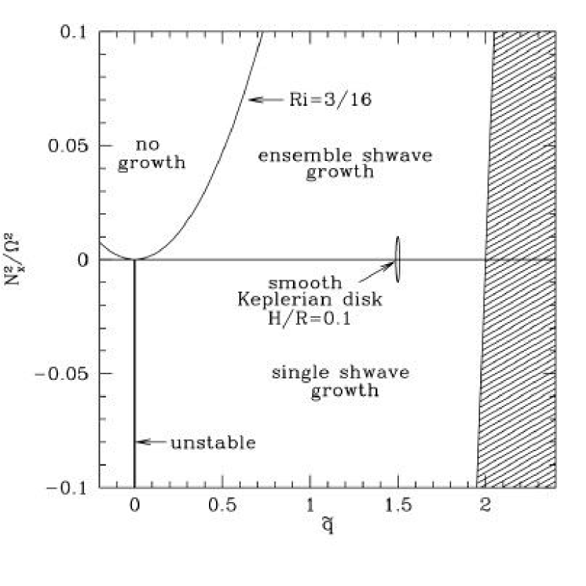
Figure 3.1: A summary of analytic results for shwaves (shearing waves) in a stratified disk. The relevant parameters are the local dimensionless shear rate $\tilde{q}=-\frac{1}{2}d\ln\Omega^{2}/d\ln r$ and the dimensionless Brunt-Väisälä frequency $N_{x}^{2}/\Omega^{2}$. The expected location of a thin, smooth disk is shown as a vertically extended ellipse near $\tilde{q}=1.5$, $N_{x}^{2}/\Omega^{2}=0$. The far right region (shaded in the figure) is forbidden by the Høiland criterion. When $\tilde{q}=0$ shear is absent and a modal analysis is possible; instability is present for $N_{x}^{2}<0$. Solitary shwaves with ${\rm Ri}=N_{x}^{2}/(\tilde{q}^{2}\Omega^{2})<0$ experience asymptotic power-law growth ($\propto t^{-{\rm Ri}}$ for small ${\rm Ri}$); since each shwave grows the energy of an ensemble of shwaves does as well. For $0<{\rm Ri}<3/16$ solitary shwaves decay but the energy of an ensemble of shwaves grows as a power-law in time. For ${\rm Ri}>3/16$ both solitary shwaves and the energy of an ensemble of shwaves asymptotically decay.

The presence of power-law growth of incompressive shwaves in stratified disks opens the possibility of a transition to turbulence as amplified shwaves enter the nonlinear regime. Any such transition would depend, however, on the nonlinear behavior of the disk after the shwaves break. It is far from clear that they would continue to grow. We will evaluate the nonlinear behavior of the disk in subsequent work.

Our results are essentially in agreement with the numerical results presented by Klahr [2004], that is, we find that arbitrarily large amplification factors can be obtained by starting with appropriate initial conditions. Our results, however, clarify the nature and asymptotic time dependence of the growth. Our results on the unstratified shearing sheet are also consistent with the results of Shepherd [1985] and Afshordi et al. [2004], who find that an isotropic ensemble of incompressive shwaves have fixed energy.

Chapter 4 Nonlinear Stability of Thin, Radially-Stratified Disks

4.1 Chapter Overview

We perform local numerical experiments to investigate the nonlinear stability of thin, radially-stratified disks. We demonstrate the presence of radial convective instability when the disk is nearly in uniform rotation, and show that the net angular momentum transport is slightly inwards, consistent with previous investigations of vertical convection. We then show that a convectively-unstable equilibrium is stabilized by differential rotation. Convective instability (corresponding to ${\rm Ri}\rightarrow-\infty$, where Ri is the radial Richardson number) is suppressed when ${\rm Ri}\gtrsim-1$, i.e. when the shear rate becomes greater than the growth rate. Disks with a nearly-Keplerian rotation profile and radial gradients on the order of the disk radius have ${\rm Ri}\gtrsim-0.01$ and are therefore stable to local nonaxisymmetric disturbances. One implication of our results is that the “Global Baroclinic Instability” claimed by Klahr and Bodenheimer [2003] is either global or nonexistent.

4.2 Introduction

In order for astrophysical disks to accrete, angular momentum must be removed from the disk material and transported outwards. In many disks, this outward angular momentum transport is likely mediated internally by magnetohydrodynamic (MHD) turbulence driven by the magnetorotational instability (MRI; see Balbus and Hawley 1998). A key feature of this transport mechanism is that it arises from a local shear instability and is therefore very robust. In addition, MHD turbulence transports angular momentum outwards; some other forms of turbulence, such as convective turbulence, appear to transport angular momentum inwards [Stone and Balbus, 1996]. The mechanism is only effective, however, if the plasma in the disk is sufficiently ionized to be well-coupled to the magnetic field (see §1.3.2). In portions of disks around young, low-mass stars, in cataclysmic-variable disks in quiescence, and in X-ray transients in quiescence [Stone et al., 2000, Gammie and Menou, 1998, Menou, 2000], the plasma may be too neutral for the MRI to operate. This presents some difficulties for understanding the evolution of these systems, since no robust transport mechanism akin to MRI-induced turbulence has been established for purely-hydrodynamic Keplerian shear flows.

Such a mechanism has been claimed recently by Klahr and Bodenheimer [2003], who find vortices and an outward transport of angular momentum in the nonlinear outcome of their global simulations. The claim is that this nonlinear outcome is due to a local instability (the “Global Baroclinic Instability”) resulting from the presence of an equilibrium entropy gradient in the radial direction. The instability mechanism invoked [Klahr, 2004] is an interplay between transient amplification of linear disturbances and nonlinear effects. The existence of such a mechanism would have profound implications for understanding the evolution of weakly-ionized disks.

In Chapter 3, we have performed a linear stability analysis for local nonaxisymmetric disturbances in the shearing-wave formalism. While the linear theory uncovers no exponentially-growing instability (except for convective instability in the absence of shear), interpretation of the results is somewhat difficult due to the nonnormal nature of the linear differential operators: one has a coupled set of differential equations in time rather than a dispersion relation, which results in a nontrivial time dependence for the perturbation amplitudes $\delta(t)$. In addition, transient amplification does occur for a subset of initial perturbations, and linear theory cannot tell us what effect this will have on the nonlinear outcome. For these reasons, and in order to test for the presence of local nonlinear instabilities, we here supplement our linear analysis with local numerical experiments.

We begin in §2 by outlining the basic equations for a local model of a thin disk. In §3 we summarize the linear theory results from Chapter 3. We describe our numerical model and nonlinear results in §§4 and 5, and discuss the implications of our findings in §6.

4.3 Basic Equations

The simulations of Klahr and Bodenheimer [2003] are two-dimensional (without vertical structure), since the salient feature supposedly giving rise to the instability is a radial entropy gradient. The simplest model to use for a local verification of their global results is the two-dimensional shearing sheet (see, e.g., Goldreich and Tremaine 1978). This local approximation is made by expanding the equations of motion in the ratio of the disk scale height $H$ to the local radius $R$, and is therefore only valid for thin disks ($H/R\ll 1$). The vertical structure is removed by using vertically-integrated quantities for the fluid variables. The basic equations that one obtains are

$$\frac{d\Sigma}{dt}+\Sigma\mbox{\boldmath$\nabla$}\cdot\mbox{\boldmath$v$}=0,$$ (4.1)

$$\frac{d\mbox{\boldmath$v$}}{dt}+\frac{\mbox{\boldmath$\nabla$}P}{\Sigma}+2\mbox{\boldmath$\Omega$}\times\mbox{\boldmath$v$}-2q\Omega^{2}x\hat{\mbox{\boldmath$x$}}=0,$$ (4.2)

$$\frac{d\,{\rm{ln}}S}{dt}=0,$$ (4.3)

where $\Sigma$ and $P$ are the two-dimensional density and pressure, $S\equiv P\Sigma^{-\gamma}$ is the fluid entropy, $v$ is the fluid velocity and $d/dt$ is the Lagrangian derivative. The third and fourth terms in equation (4.2) represent the Coriolis and centrifugal forces in the local model expansion, where $\Omega$ is the local rotation frequency, $x$ is the radial Cartesian coordinate and $q$ is the shear parameter (equal to $1.5$ for a disk with a Keplerian rotation profile). The gravitational potential of the central object is included as part of the centrifugal force term in the local-model expansion, and we ignore the self-gravity of the disk.

4.4 Summary of Linear Theory Results

An equilibrium solution to equations (4.1) through (4.3) is

$$P=P_{0}(x),$$ (4.4)

$$\Sigma=\Sigma_{0}(x),$$ (4.5)

$$\mbox{\boldmath$v$}\equiv\mbox{\boldmath$v$}_{0}=\left(-q\Omega x+\frac{P_{0}^{\prime}}{2\Omega\Sigma_{0}}\right)\hat{\mbox{\boldmath$y$}},$$ (4.6)

where a prime denotes an $x$ derivative. One can regard the background flow as providing an effective shear rate

$${\tilde{q}}\Omega\equiv-v_{0}^{\prime}$$ (4.7)

that varies with $x$, in which case $\mbox{\boldmath$v$}_{0}=-\int^{x}{\tilde{q}}(s)ds\,\Omega\hat{\mbox{\boldmath$y$}}$. Due to this background shear, localized disturbances can be decomposed in terms of “shwaves”, Fourier modes in a frame comoving with the shear. These have a time-dependent radial wavenumber given by

$$\tilde{k}_{x}(t,x)\equiv k_{x0}+{\tilde{q}}(x)\Omega k_{y}t.$$ (4.8)

where $k_{x0}$ and $k_{y}$ are constants. Here $k_{y}$ is the azimuthal wave number of the shwave.

In the limit of zero stratification,

$$P_{0}(x)\rightarrow constant,$$ (4.9)

$$\Sigma_{0}(x)\rightarrow constant,$$ (4.10)

$$\mbox{\boldmath$v$}_{0}\rightarrow-q\Omega x\hat{\mbox{\boldmath$y$}},$$ (4.11)

$${\tilde{q}}\rightarrow q,$$ (4.12)

and

$$\tilde{k}_{x}\rightarrow k_{x}\equiv k_{x0}+q\Omega k_{y}t.$$ (4.13)

In Chapter 3, we analyze the time dependence of the shwave amplitudes for both an unstratified equilibrium and a radially-stratified equilibrium. As discussed in more detail in Chapter 3, applying the shwave formalism to a radially-stratified shearing sheet effectively uses a short-wavelength WKB approximation, and is therefore only valid in the limit $k_{y}L\gg 1$, where the background varies on a scale $L\sim H\ll R$. The disk scale height $H\equiv c_{s}\Omega$, where $c_{s}=\sqrt{\gamma P_{0}/\Sigma_{0}}$.

There are three nontrivial shwave solutions in the unstratified shearing sheet, two nonvortical and one vortical. The radial stratification gives rise to an additional vortical shwave. In the limit of tightly-wound shwaves ($|k_{x}|\gg k_{y}$), the nonvortical and vortical shwaves are compressive and incompressive, respectively. The former are the extension of acoustic modes to nonaxisymmetry, and to leading order in $(k_{y}L)^{-1}$ they are the same both with and without stratification. Since the focus of our investigation is on convective instability and the generation of vorticity, we repeat here only the solutions for the incompressive vortical shwaves and refer the reader to Chapter 3 for further details on the nonvortical shwaves.

In the unstratified shearing sheet, the solution for the incompressive shwave is given by:

$$\delta v_{x}=\delta v_{x0}\frac{k_{0}^{2}}{k^{2}},$$ (4.14)

$$\delta v_{y}=-\frac{k_{x}}{k_{y}}\delta v_{x}$$ (4.15)

and

$$\frac{\delta\Sigma}{\Sigma_{0}}=\frac{\delta P}{\gamma P_{0}}=\frac{1}{ic_{s}k_{y}}\left(\frac{k_{x}}{k_{y}}\frac{\dot{\delta v}_{x}}{c_{s}}+2(q-1)\Omega\frac{\delta v_{x}}{c_{s}}\right),$$ (4.16)

where $k^{2}=k_{x}^{2}+k_{y}^{2}$, ($k_{0},\delta v_{x0}$) are the values of ($k,\delta v_{x}$) at $t=0$ and an overdot denotes a time derivative.

The kinetic energy for a single incompressive shwave can be defined as

$$E_{k}\equiv\frac{1}{2}\Sigma_{0}(\delta v_{x}^{2}+\delta v_{y}^{2})=\frac{1}{2}\Sigma_{0}\delta v_{x0}^{2}\frac{k_{0}^{4}}{k_{y}^{2}k^{2}},$$ (4.17)

an expression which varies with time and peaks at $k_{x}=0$. If one defines an amplification factor for an individual shwave,

$${\cal A}\equiv\frac{E_{k}(k_{x}=0)}{E_{k}(t=0)}=1+\frac{k_{x0}^{2}}{k_{y}^{2}},$$ (4.18)

it is apparent that an arbitrary amount of transient amplification in the kinetic energy of an individual shwave can be obtained as one increases the amount of swing for a leading shwave ($k_{x0}\ll-k_{y}$).

This transient amplification of local nonaxisymmetric disturbances is reminiscent of the “swing amplification” mechanism that occurs in disks that are marginally-stable to the axisymmetric gravitational instability [Goldreich and Lynden-Bell, 1965, Julian and Toomre, 1966, Goldreich and Tremaine, 1978]. In that context, nonaxisymmetric shwaves experience a short period of exponential growth near $k_{x}=0$ as they swing from leading to trailing. In order for this mechanism to be effective in destabilizing a disk, however, a feedback mechanism is required to convert trailing shwaves into leading shwaves [Binney and Tremaine, 1987]. The arbitrarily-large amplification implied by equation (4.18) has led some authors to argue for a bypass transition to turbulence in hydrodynamic Keplerian shear flows [Chagelishvili et al., 2003, Umurhan and Regev, 2004, Afshordi et al., 2004]. The reasoning is that nonlinear effects somehow provide the necessary feedback. We show in Chapter 3 that a ensemble of incompressive shwaves drawn from an isotropic, Gaussian random field has a kinetic energy that is a constant, independent of time. This indicates that a random set of vortical perturbations will not extract energy from the mean shear. It is clear, however, that the validity of this mechanism as a transition to turbulence can only be fully explored via numerical experiments. No numerical experiments to date have demonstrated a transition to turbulence in Keplerian shear flows.

In the presence of radial stratification, there are two linearly-independent incompressive shwaves. The radial-velocity perturbation satisfies the following equation (we use a subscript $s$ to distinguish the stratified from the unstratified case):

$$(1+\tilde{\tau}^{2})\frac{d^{2}\delta v_{xs}}{d\tilde{\tau}^{2}}+4\tilde{\tau}\frac{d\delta v_{xs}}{d\tilde{\tau}}+({\rm{Ri}}+2)\delta v_{xs}=0,$$ (4.19)

where

$$\tilde{\tau}\equiv\tilde{k}_{x}/k_{y}={\tilde{q}}\Omega t+k_{x0}/ky$$ (4.20)

is the time variable and

$${\rm Ri}\equiv\frac{N_{x}^{2}}{({\tilde{q}}\Omega)^{2}}$$ (4.21)

is the Richardson number, a measure of the relative importance of buoyancy and shear [Miles, 1961, Howard, 1961, Chimonas, 1970]. Here

$$N_{x}^{2}\equiv-\frac{c_{s}^{2}}{L_{S}L_{P}}$$ (4.22)

is the square of the Brunt-V$\ddot{\rm{a}}$is$\ddot{\rm{a}}$l$\ddot{\rm{a}}$ frequency in the radial direction, where $L_{P}\equiv\gamma P_{0}/P_{0}^{\prime}$ and $L_{S}\equiv\gamma S_{0}/S_{0}^{\prime}$ are the equilibrium pressure and entropy length scales in the radial direction. The solutions for the other perturbation variables are related to $\delta v_{xs}$ by

$$\delta v_{ys}=-\tilde{\tau}\delta v_{xs},$$ (4.23)

$$\frac{\delta\Sigma_{s}}{\Sigma_{0}}=\frac{1}{L_{S}}\int\delta v_{xs}\,dt$$ (4.24)

and

$$\frac{\delta P_{s}}{P_{0}}=\frac{\gamma\Omega}{ic_{s}k_{y}}\left[{\tilde{q}}\tilde{\tau}\frac{d}{d\tilde{\tau}}\left(\frac{\delta v_{xs}}{c_{s}}\right)+2({\tilde{q}}-1)\frac{\delta v_{xs}}{c_{s}}\right].$$ (4.25)

Since the solutions to equation (4.19) are hypergeometric functions, which have a power-law time dependence, it cannot in general be accurately treated with a WKB analysis; there is no asymptotic region in time where equation (4.19) can be reduced to a dispersion relation. If, however, there is a region of the disk where the effective shear is zero, $\tilde{\tau}\rightarrow constant$ and equation (4.19) can be expressed as a WKB dispersion relation:

$$\omega^{2}=\frac{k_{y}^{2}}{k_{x0}^{2}+k_{y}^{2}}N_{x}^{2},$$ (4.26)

with $\delta(t)\propto\exp(-i\omega t)$. For ${\tilde{q}}\simeq 0$ and $N_{x}^{2}<0$, then, there is convective instability. For disks with nearly-Keplerian rotation profiles and modest radial gradients, ${\tilde{q}}\simeq 1.5$ and one would expect that the instability is suppressed by the strong shear. Due to the lack of a dispersion relation, however, there is no clear cutoff between exponential and oscillatory time dependence, and establishing a rigorous analytic stability criterion is difficult.

For ${\tilde{q}}\neq 0$, the asymptotic time dependence for each perturbation variable at late times is

$$\delta P_{s}\propto\delta v_{xs}\sim t^{\frac{\alpha-3}{2}},$$ (4.27)

$$\delta\Sigma_{s}\propto\delta v_{ys}\sim t^{\frac{\alpha-1}{2}},$$ (4.28)

where

$$\alpha\equiv\sqrt{1-4\,{\rm{Ri}}}.$$ (4.29)

The density and $y$-velocity perturbations therefore grow asymptotically for $\alpha>1$, i.e. ${\rm{Ri}}<0$. For small Richardson number, as is expected for a nearly-Keplerian disk with modest radial gradients, $\alpha\simeq 1-2{\rm Ri}$ and the asymptotic growth is extremely slow:

$$\delta\Sigma_{s}\sim\delta v_{ys}\sim t^{-{\rm Ri}}.$$ (4.30)

The energy of an ensemble of shwaves grows asymptotically as $t^{2\alpha-1}$, or $t^{1-4{\rm Ri}}$ for small Ri. The ensemble energy growth is thus nearly linear in time for small Ri, independent of the sign of Ri.

The velocity perturbations are changed very little by a weak radial gradient. One would therefore expect that, at least in the linear regime, transient amplification of the kinetic energy for an individual shwave is relatively unaffected by the presence of stratification. There is, however, an associated density perturbation in the stratified shearing sheet that is not present in the unstratifed sheet. This results in transient amplification of the potential energy of an individual shwave. We do not derive in Chapter 3 I a general closed-form expression for the energy of an ensemble of incompressive shwaves in the stratified shearing sheet, so it is not entirely clear what effect this qualitatively new piece of the energy will have on an ensemble of shwaves in the linear regime.

In any case, the question of whether or not radial stratification can play a role in generating turbulence by interacting with the transient amplification of linear disturbances or by some other nonlinear mechanism can only be fully answered with a nonlinear study. For this reason, and due to the subtleties involved in the linear analysis, we now turn to the main focus of this paper, which is a series of local numerical experiments in a radially-stratified shearing sheet.

4.5 Numerical Model

To investigate local nonlinear effects in a radially-stratified thin disk, we integrate the governing equations (4.1) through (4.3) with a hydrodynamics code based on ZEUS [Stone and Norman, 1992]. This is a time-explicit, operator-split, finite-difference method on a staggered mesh. It uses an artificial viscosity to capture shocks. The computational grid is $L_{x}\times L_{y}$ in physical size with $N_{x}\times N_{y}$ grid cells, where $x$ is the radial coordinate and $y$ is the azimuthal coordinate. The boundary conditions are periodic in the $y$-direction and shearing-periodic in the $x$-direction. The shearing-box boundary conditions are described in detail in Hawley et al. [1995]. As described in Masset [2000] and Gammie [2001], advection by the linear shear flow can be done by interpolation. Rather than using a linear interpolation scheme as in Gammie [2001], we now do the shear transport with the same upwind advection algorithm used in the rest of the code. This is less diffusive than linear interpolation, and the separation of the shear from the bulk fluid velocity means that one is not Courant-limited by large shear velocities at the edges of the computational domain.

We use the following equilibrium profile, which in general gives rise to an entropy that varies with radius:

$$h_{0}(x)=h_{a}\left[1-\epsilon\cos\left(\frac{2\pi x}{L_{x}}\right)\right]\;\;,\;\;\Sigma_{0}(x)=\left[\frac{h_{0}(\Gamma-1)}{\Gamma K}\right]^{\frac{1}{\Gamma-1}}\;\;,\;\;P_{0}(x)=K\Sigma_{0}^{\Gamma},$$ (4.31)

where $h_{a}$, $\epsilon$, $\Gamma$ and $K$ are model parameters. The flow is maintained in equilibrium by setting the initial velocity according to equation (4.6). This equilibrium yields a Brunt-V$\ddot{\rm{a}}$is$\ddot{\rm{a}}$l$\ddot{\rm{a}}$ frequency

$$N_{x}^{2}(x)=\frac{(\gamma-\Gamma){h_{0}^{\prime}}^{2}}{\gamma(\Gamma-1)h_{0}},$$ (4.32)

which can be made positive, negative or zero by varying $\gamma-\Gamma$.

We fix some of the model parameters to yield an equilibrium profile that is appropriate for a thin disk. In particular, we want $H/L_{P}\sim H/R\ll 1$ in order to be consistent with our use of a razor-thin (two-dimensional) disk model. In addition, we want the equilibrium values for each fluid variable to be of the same order to ensure the applicability of our linear analysis. These requirements can be met by choosing $K=1$, $\epsilon=0.1$, $L_{x}=12$ and $h_{a}=\bar{c}_{s}^{2}\Gamma/(\Gamma-1)$, where $\bar{c}_{s}\equiv\sqrt{{\langle}P_{0}/\Sigma_{0}{\rangle}}\equiv 1$ is (to within a factor of $\sqrt{\gamma}$) the $x$ average of the sound speed. Since the equilibrium profile changes with $\Gamma$, we choose a fixed value of $\Gamma=4/3$, which for $\gamma=\Gamma$ corresponds to a three-dimensional adiabatic index of $7/5$. These numbers yield $|H/L_{P}|\leq 0.2$. Our unfixed model parameters are thus $L_{y}$, $q$ and $\gamma$.

The sinusoidal equilibrium profile we are using generates radial oscillations in the shearing sheet due to truncation error. We apply an exponential-damping term to the governing equations in order to reduce the spurious oscillations and therefore get cleaner growth-rate measurements. We damp the oscillations until their amplitude is equal to that of machine-level noise, and subsequently apply low-level random perturbations to trigger any instabilities that may be present.

As a test for our code, we evolve a particular solution for the incompressive shwaves in the radially-stratified shearing sheet (equations [4.19] and [4.23]-[4.25]). The initial conditions are $\delta v_{x}/\bar{c}_{s}=\delta\Sigma/\Sigma_{0}=1\times 10^{-4}$ and $k_{x0}=-128\pi/L_{x}$. We set $L_{y}=0.375$ and $k_{y}=2\pi/L_{y}$ in order to operate in the short-wavelength regime, and the other model parameters are $q=1.5$ and $\gamma-\Gamma=-0.3102$. The latter value yields a minimum value for $N_{x}^{2}(x)$ of $-0.01$. The results of the linear theory test are shown in Figures 4.2 and 4.2.

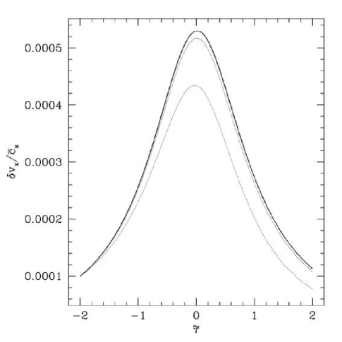
Figure 4.1: Evolution of the radial velocity amplitude for a vortical shwave in the radially-stratified shearing sheet (Run 1). The heavy line is the analytic result, and the light lines are runs with a numerical resolution of (in order of increasing accuracy) $N_{x}\times N_{y}=1024\times 16$, $2048\times 32$ and $4096\times 64$. The number of grid cells are chosen so that the shwave initially has the same number of grid cells per wavelength in both the $x$ and $y$ directions. The results are shown for a test point at the minimum in $N_{x}^{2}$.

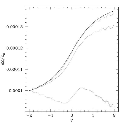
Figure 4.2: Evolution of the density amplitude for a vortical shwave in the radially-stratified shearing sheet (Run 1). The heavy line is the analytic result, and the light lines are runs with a numerical resolution of (in order of increasing accuracy) $N_{x}\times N_{y}=1024\times 16$, $2048\times 32$ and $4096\times 64$.

4.6 Nonlinear Results

Table 4.1: Summary of Code Runs

Run	Description	Figure(s)
1	Linear theory test	4.2-4.2
2	External potential, $\Omega=0$	4.3-4.6
3	External potential, $\Omega=1$	4.7-4.8
4	Uniform rotation ($q=0$)	4.9-4.11
5	External potential, $\Omega=1$, boost	4.12
6	Small shear ($-\infty\lesssim{\rm Ri}\lesssim-1$)	4.13
7	Small shear ($q=0.2,{\rm Ri}\gtrsim-1$)	4.14
8	Aliasing ($q=0.2,{\rm Ri}\gtrsim-1$)	4.15
9	Parameter survey	4.16
10	Keplerian disk ($q=1.5,{\rm Ri}\simeq-0.004$)	4.17

Table 4.1 gives a summary of the runs that we have performed. A detailed description of the setup and results for each is given in the following subsections. Our primary diagnostic is a measurement of growth rates, and the probe that we use for these measurements is an average over azimuth of the absolute value of $v_{x}=\delta v_{x}$ at the minimum in $N_{x}^{2}$. Measuring $v_{x}$ allows us to demonstrate the damping of the initial radial oscillations, and the average over azimuth masks the interactions between multiple WKB modes with different growth rates in our measurements. We will reference this probe with the following definition:

$$v_{t}\equiv\langle|v_{x}(x_{min},y)|\rangle,$$ (4.33)

where here angle brackets denote an average over $y$ and $x_{min}$ is the $x$-value at which $N_{x}^{2}(x)$ is a minimum.

4.6.1 External Potential in Non-Rotating Frame

As a starting problem, we investigate a stratified flow with $\mbox{\boldmath$v$}_{0}=0$. Such a flow can be maintained in equilibrium by replacing the tidal force in equation (4.2) with an external potential $\Phi=-h_{0}$. This can be done in either a rotating or non-rotating frame. It is a particularly simple way of validating our study of convective instability in the shearing sheet. The condition $\mbox{\boldmath$v$}_{0}=0$ implies ${\tilde{q}}=0$, and therefore equation (4.26) should apply in the WKB limit, with the expected growth rate obtained by evaluating equation (4.32) locally. We have performed a fiducial run with an imposed external potential in a non-rotating frame ($\Omega=0$ in equation [4.2]) to compare with the outcome expected from the Schwarzschild stability criterion implied by equation (4.26). We set $\gamma-\Gamma=-0.3102$, corresponding to $N_{x,min}^{2}=-0.01$, and $L_{y}=L_{x}$. The expected growth rate for this Schwarzschild-unstable equilibrium is $0.1$ (in units of the average radial sound-crossing time). The numerical resolution for the fiducial run is $512\times 512$, and all the variables are randomly perturbed at an amplitude of $1.0\times 10^{-12}$.

A plot of $v_{t}$ as a function of time is given in Figure 4.3, showing the initial damping followed by exponential growth in the linear regime. The analytic growth rate is shown on the plot for comparison. A least-squares fit of the data in the range $100\leq t\leq 250$ yields a measured growth rate of $0.0978$. Figure 4.5 shows a cross section of $N_{x}^{2}$ as a function of $x$ after the instability has begun to set in, and Figure 4.5 shows cross sections of the entropy early and late in the nonlinear regime. The growth is initially concentrated near the minimum points in $N_{x}^{2}(x)$. Eventually the entropy turns over completely and settles to a nearly constant value. Figure 4.6 shows two-dimensional snapshots of the entropy in the nonlinear regime. Runs with the same equilibrium profile except $\gamma-\Gamma\geq 0$ are stable. There is also a long-wavelength axisymmetric instability that is present for $\gamma-\Gamma<0$ even in the absence of the small-scale nonaxisymmetric modes. We measure its growth rate to be $0.07$. Due to the long-wavelength nature of these modes, they are not treatable by a local linear analysis.

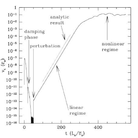
Figure 4.3: Evolution of $v_{t}$ as a function of time for Run 2 (external potential, non-rotating frame).

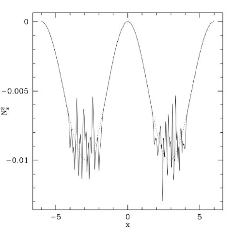
Figure 4.4: Plot of $N_{x}^{2}$ (averaged over $y$) as a function of $x$ for Run 2. The dotted line shows the equilibrium profile, and the solid line shows a snapshot during the nonlinear regime. Growth initially occurs at the minimum in $N_{x}^{2}$.

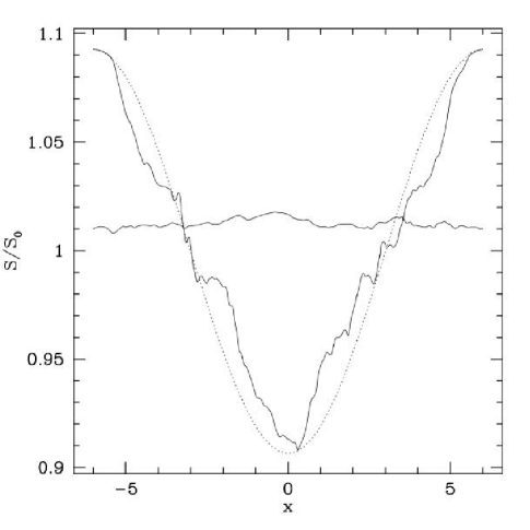
Figure 4.5: Plot of the entropy (averaged over $y$) as a function of $x$ for Run 2. The dotted line shows the equilibrium profile, and the solid lines show snapshots during the nonlinear regime. The entropy eventually settles to a nearly-constant value.

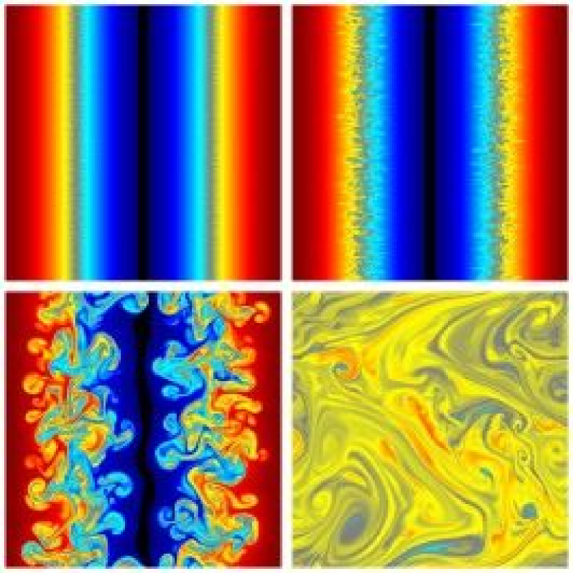
Figure 4.6: Snapshots of the entropy in the nonlinear regime for Run 2, indicating maximum growth for modes near the grid scale and the eventual turnover of the equilibrium entropy profile to its average value. Dark shades indicate values above (red in the color version) and below (blue in the color version) the average value (yellow in the color version).

4.6.2 External Potential in Rotating Frame

We have performed the same test as described in §5.1 in a rotating frame ($\Omega=1$ in equation [4.2]). Figure 4.7 shows the exponential growth in the linear regime for this run, with a measured growth rate of $0.0977$. Figure 4.8 shows snapshots of the entropy in the nonlinear regime. The results are similar to the nonrotating case, except that 1) rotation suppresses the long-wavelength axisymmetric instability; 2) the nonlinear outcome exhibits more coherent structures in the rotating case including transient vortices; and 3) these coherent structures eventually become unstable to a Kelvin-Helmholz-type instability.

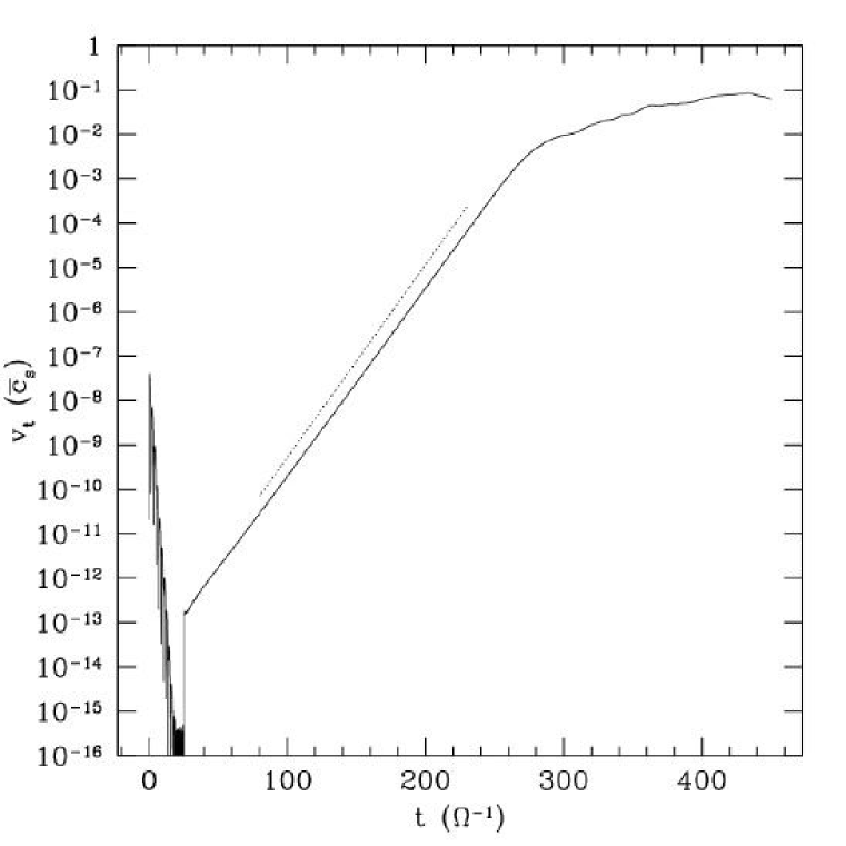
Figure 4.7: Evolution of $v_{t}$ as a function of time for Run 3 (external potential, rotating frame). The dotted line shows the expected growth rate.

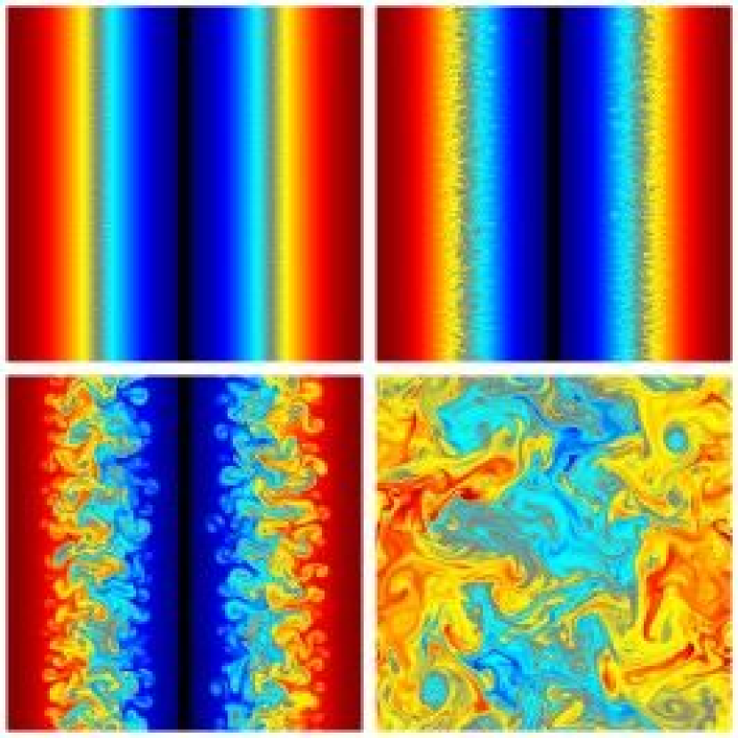
Figure 4.8: Snapshots of the entropy in the nonlinear regime for Run 3. Dark shades indicate values above (red in the color version) and below (blue in the color version) the average value (yellow in the color version).

4.6.3 Uniform Rotation

Having demonstrated the viability of simulating convective instability in the local model, we now turn to the physically-realistic equilibrium described in §4. We begin by setting the shear parameter $q$ to zero in order to make contact with the results of §§5.1 and 5.2. This is analogous to a disk in uniform rotation. The other model parameters are the same as for the previous runs. While there is still an effective shear $-0.05\lesssim{\tilde{q}}\lesssim 0.05$, near ${\tilde{q}}=0$ one expects the modes to obey equation (4.26) in the WKB limit. Figures 4.9 and 4.10 give the linear and nonlinear results for this run. The measured growth rate in the linear regime is $0.0809$.

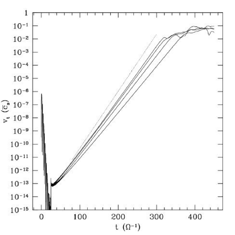
Figure 4.9: Evolution of $v_{t}$ as a function of time for Run 4 ($q=0$). The dotted line shows the expected growth rate, and the solid lines are runs with (in order of increasing growth) $L_{y}=12$, $6$, $3$ and $1.5$.

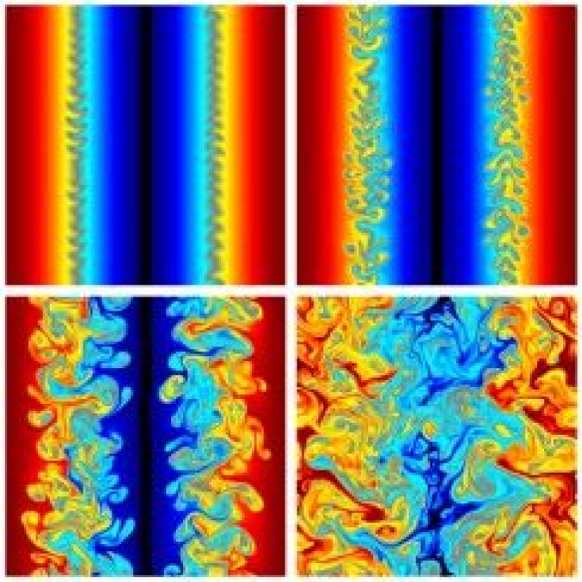
Figure 4.10: Snapshots of the entropy in the nonlinear regime for Run 4. Notice that the maximum growth does not occur for modes at the grid scale.

Consistent with results from numerical simulations of vertical convection [Stone and Balbus, 1996, Cabot, 1996], the angular momentum transport associated with radial convection is inwards. Figure 4.11 shows the evolution of the dimensionless angular momentum flux

$$\alpha\equiv\frac{1}{L_{x}L_{y}{\langle}P_{0}{\rangle}}\int\Sigma\delta v_{x}\delta v_{y}dxdy,$$ (4.34)

where ${\langle}P_{0}{\rangle}$ is the radial average of the equilibrium pressure, for an extended version of Run 4. Averaging over the last $1200\Omega^{-1}$ yields $\alpha\sim-10^{-5}$.

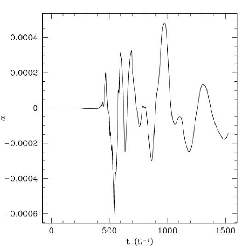
Figure 4.11: Evolution of the dimensionless angular momentum flux due to radial convection.

There are two reasons for the larger error in the measured growth rate for this run: 1) the equilibrium velocity gives rise to numerical diffusion due to the motion of the fluid variables with respect to the grid; and 2) since the growing modes are being advected in the azimuthal direction, the maximum growth does not occur at the grid scale. The latter effect can be seen in Figure 4.10; several grid cells are required for a well-resolved wavelength. In order to resolve smaller wavelengths, we have repeated this run with $L_{y}=6$, $3$ and $1.5$. The results are plotted in Figure 4.9 along with the results from the $L_{y}=12$ run. The measured growth rate for the $L_{y}=1.5$ run is $0.0924$.

To quantify the effects of numerical diffusion, we have performed a series of tests similar to Run 2 (external potential in a rotating frame) but with an overall boost in the azimuthal direction. Figure 4.12 shows measured growth rates as a function of boost at three different numerical resolutions. The largest boost magnitude in this plot corresponds to the velocity at the minimum in $N_{x}^{2}$ for a run with $q=1.5$.

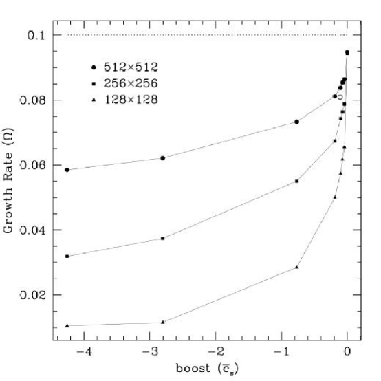
Figure 4.12: Growth rates as a function of azimuthal boost in a series of runs with an external potential and $N_{x,min}^{2}=-0.01$. The dotted line shows the analytic growth rate from linear theory. The open circle denotes the growth rate that was measured in Run 4, with the boost corresponding to the magnitude of the velocity at the minimum in $N_{x}^{2}$ for Run 3 ($q=0$). The largest boost magnitude corresponds to the velocity at the minimum in $N_{x}^{2}$ for Run 10 ($q=1.5$).

4.6.4 Shearing Sheet

To investigate the effect of differential rotation upon the growth of this instability, we have performed a series of simulations with nonzero $q$. Intuitively, one expects the instability to be suppressed when the shear rate is greater than the growth rate, i.e. for ${\rm Ri}\gtrsim-1$. Figure 4.13 shows growth rates from a series of runs with $N_{x,min}^{2}=-0.01$ and small, nonzero values of $q$ at three numerical resolutions. This figure clearly demonstrates our main result: convective instability is suppressed by differential rotation. The expected growth rate from linear theory ($\sqrt{|N_{x}^{2}|}$ at ${\tilde{q}}=0$) is shown in Figure 4.13 as a dotted line. If there is a radial position where ${\tilde{q}}(x)=0$ (i.e., ${\rm Ri}=-\infty$), $v_{t}$ at that position looks similar to that of the previous runs (very little deviation from a straight line); these measurements are indicated on the plot with solid points. For $q\gtrsim 0.055$ there is no longer any point where ${\tilde{q}}(x)=0$; in that case $v_{t}$ was measured at the radial average between the minimum in $N_{x}^{2}(x)$ and the minimum in ${\tilde{q}}(x)$, since this is where the maximum growth occured. The data for these measurements, which are indicated in Figure 4.13 with open points, is not as clean as it is for the runs with ${\rm Ri}=-\infty$ (see Figure 4.14). All of the growth rate measurements in Figure 4.13 were obtained by a least-squares fit of the data in the range $1\times 10^{-9}<v_{t}/\bar{c}_{s}<1\times 10^{-5}$. The dashed line in Figure 4.13 indicates the value of $q$ for which ${\rm Ri}_{min}=-1$.

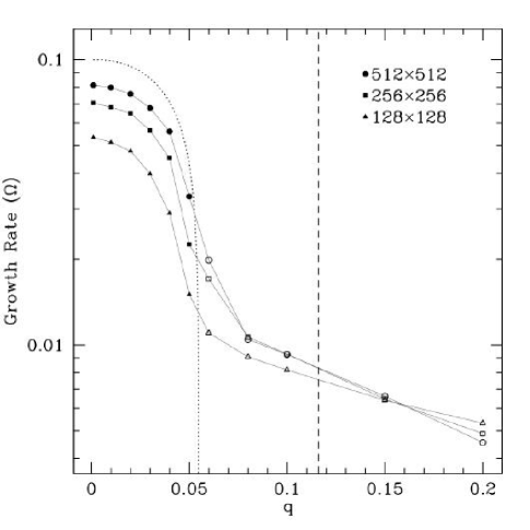
Figure 4.13: Growth rates as a function of $q$ with $N_{x,min}^{2}=-0.01$. See the text for a discussion.

Some of the growth in Figure 4.13 appears to be due to aliasing. This is a numerical effect in finite-difference codes that results in an artificial transfer of power from trailing shwaves into leading shwaves as the shwave is lost at the grid scale. One expects aliasing to occur approximately at intervals of

$$\Delta\tilde{\tau}=\frac{N_{x}}{n_{y}}\frac{L_{y}}{L_{x}},$$ (4.35)

where $n_{y}$ is the azimuthal shwave number. This interval corresponds to $\Delta\tilde{k}_{x}(t)=2\pi/dx$, where $dx=L_{x}/N_{x}$ is the radial grid scale. Based upon expression (4.35), aliasing effects should be more pronounced at lower numerical resolution because the code has less time to evolve a shwave before the wavelength of the shwave becomes smaller than the grid scale. It can be seen from the far-right data point in Figure 4.13 (Run 7 in Table 4.1) that the measured growth rate decreases with increasing resolution. The evolution of $v_{t}$ for this run is shown in Figure 4.14.

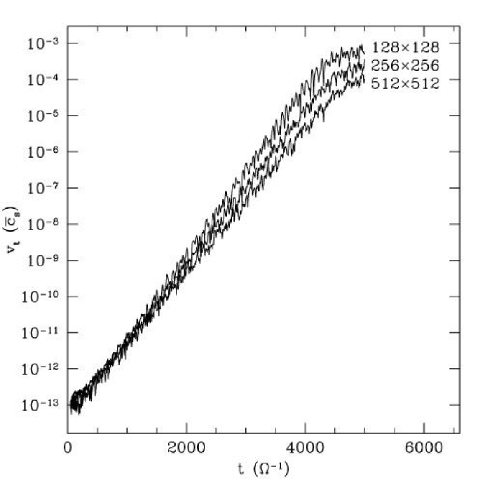
Figure 4.14: Evolution of $v_{t}$ as a function of time for Run 7 ($q=0.2$ and $N_{x,min}^{2}=-0.01$).

The effects of aliasing can be seen explicitly by evolving a single shwave, as was done for our linear theory test (Figures 4.2 and 4.2). Figure 4.15 shows the evolution of the density perturbation for a single shwave using the same parameters that were used for Run 7: $L_{x}=L_{y}=12$, $N_{x,min}^{2}=-0.01$ and $q=0.2$. The initial shwave vector used was $(k_{x0},k_{y})=(-8\pi/L_{x},8\pi/L_{y})$. This corresponds to $n_{y}=4$, and the expected aliasing interval (4.35) is therefore $\Delta\tilde{\tau}=N_{x}/4$. Runs at three numerical resolutions are plotted in Figure 4.15, and the aliasing interval at each resolution is consistent with expression (4.35). It is clear from Figure 4.15 that a lower resolution results in a larger overall growth at the end of the run. It also appears that the growth seen in Figure 4.15 requires a negative entropy gradient. We have performed this same test with $N_{x}^{2}>0$, and while aliasing occurs at the same interval, there is no overall growth in the perturbations. This is likely due to the fact that the perturbations decay asymptotically for $N_{x}^{2}>0$ (see expression [4.30]).

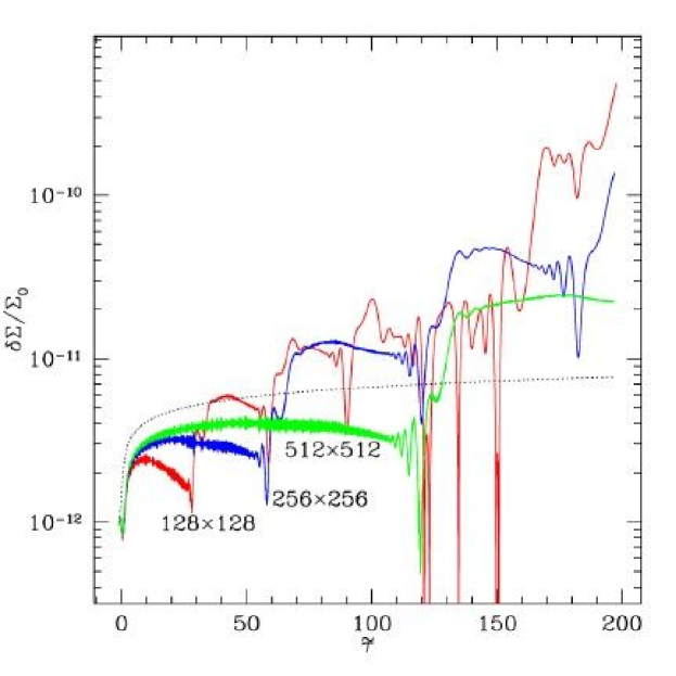
Figure 4.15: Evolution of the density perturbation for a single shwave with $q=0.2$, $N_{x,min}^{2}=-0.01$ and $L_{y}=L_{x}$ (Run 8). The linear theory result is shown as a dotted line, along with results at three numerical resolutions. Aliasing occurs when $\tilde{k}_{x}(t)=2\pi/dx$. The overall growth, which is greater at lower numerical resolution, requires $N_{x}^{2}<0$.

Figure 4.16 summarizes the parameter space we have surveyed, indicating that there is instability only for ${\tilde{q}}\simeq 0$ and $N_{x}^{2}<0$. The numerical resolution in all of these runs is $512\times 512$. Figure 4.17 shows the evolution of the radial velocity in Run 10, a run with realistic parameters for a disk with a nearly-Keplerian rotation profile and radial gradients on the order of the disk radius: $q=1.5$ and $N_{x,min}^{2}=-0.01$ (corresponding to ${\rm Ri}\simeq-0.004$). Clearly no instability is occurring on a dynamical timescale. This plot is typical of all runs for which the evolution was stable. To give a sense for the minimum growth rate that we are able to measure, we have also plotted in Figure 4.17 the results from several unstable runs with $q=0$ and a boost equivalent to the velocity at the minimum in $N_{x}^{2}$ for Run 10. It is difficult to measure a growth rate for the smallest value of $N_{x,min}^{2}$, but it is clear that there is activity present in this run which does not occur in the stable run. Based upon Figure 4.17, a conservative estimate for the minimum growth rate that should be detectable in our simulations is $0.0025\Omega$.

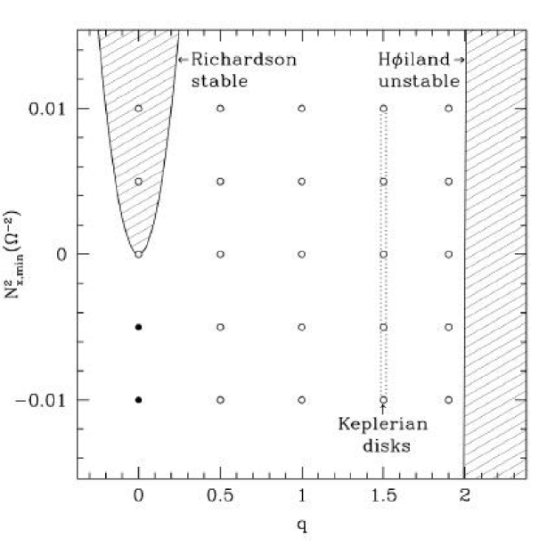
Figure 4.16: Parameter space surveyed in a search for nonlinear instabilities. Closed (open) circles denote runs that were unstable (stable). The only instability found was convective instability for ${\tilde{q}}\simeq 0$ and $N_{x}^{2}<0$ (${\rm Ri}\rightarrow-\infty$). (We do not include on this plot the runs shown in Figure 4.13.)

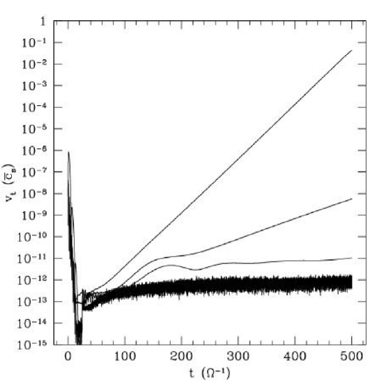
Figure 4.17: Evolution of $v_{t}$ as a function of time for Run 10 ($q=1.5$, $N_{x,min}^{2}=-0.01$). Also shown are runs with $q=0$ and an overall boost equivalent to the velocity at the minimum in $N_{x}^{2}$ for Run 10, for $N_{x,min}^{2}=-0.01$ (measured growth rate of $0.058$), $N_{x,min}^{2}=-0.003$ (measured growth rate of $0.021$) and $N_{x,min}^{2}=-0.001$ (measured growth rate of $0.0025$).

4.7 Implications

Our results seem to indicate that nearly-Keplerian disks with weak radial gradients are stable to local nonaxisymmetric disturbances, although we cannot exclude instability at very high Reynolds number. Figure 4.13 demonstrates that convective instability, present when the shear is nearly zero, is stabilized by differential rotation. Perturbations simply do not have time to grow before they are pulled apart by the shear.

An important implication of our results is that the instability claimed by Klahr and Bodenheimer [2003] is not a linear or nonlinear local nonaxisymmetric instability. Figure 4.15 suggests that the results of Klahr and Bodenheimer [2003] may be due, at least in part, to aliasing. They use a finite difference code at fairly low numerical resolution ($\leq 128^{2}$), and growth is only observed in runs with a negative entropy gradient. Curvature effects and the effects of boundary conditions, which may also play a role in their global results, cannot be tested in our local model.

Chapter 5 Vortices in Thin, Compressible, Unmagnetized Disks

5.1 Chapter Overview

We consider the formation and evolution of vortices in a hydrodynamic shearing-sheet model. The evolution is done numerically using a version of the ZEUS code. Consistent with earlier results, an injected vorticity field evolves into a set of long-lived vortices each of which has radial extent comparable to the local scale height. But we also find that the resulting velocity field has positive shear stress ${\langle}\Sigma\delta v_{r}\delta v_{\phi}{\rangle}$. This effect appears only at high resolution. The transport, which decays with time as $t^{-1/2}$, arises primarily because the vortices drive compressive motions. This result suggests a possible mechanism for angular momentum transport in low-ionization disks, with two important caveats: a mechanism must be found to inject vorticity into the disk, and the vortices must not decay rapidly due to three-dimensional instabilities.

5.2 Introduction

Astrophysical disks are common because the specific angular momentum of the matter inside them is well-conserved. They evolve because angular momentum conservation is weakly compromised, either because of diffusion of angular momentum within the disk or because of direct application of external torques.

In astrophysical disks composed of a well-ionized plasma it is likely that some, perhaps most, of the evolution is driven by diffusion of angular momentum within the disk. This view is certainly consistent with observations of steadily accreting cataclysmic variable systems like UX Ursa Majoris [Baptista et al., 1998, Baptista, 2004], whose radial surface-brightness profile is consistent with steady accretion-flow models in which the bulk of the accretion energy is dissipated within the disk.

Angular momentum diffusion in well-ionized disks is likely driven by magnetohydrodynamic (MHD) turbulence. Analytic analyses, numerical experiments, and laboratory evidence strongly suggest that well-coupled plasmas in differentially-rotating flows are subject to the magnetorotational instability (MRI; Balbus and Hawley 1991, 1998, Balbus 2003). But MHD turbulence is initiated by the MRI only so long as the plasma is sufficiently ionized to couple to the magnetic field [Kunz and Balbus, 2004, Desch, 2004]. In disks around young stars, cataclysmic-variable and X-ray binary disks in quiescence, and possibly the outer parts of AGN disks, the plasma may be too neutral to support magnetic activity [Gammie and Menou, 1998, Menou, 2000, Stone et al., 2000, Menou and Quataert, 2001, Fromang et al., 2002]. This motivates interest in non-MHD angular momentum transport mechanisms.

Within the last few years, a body of work has been developed suggesting that vortices can be generated as a result of global hydrodynamic instability [Hawley, 1987, Blaes and Hawley, 1988, Hawley, 1990, Lovelace et al., 1999, Li et al., 2000] or local hydrodynamic instability [Klahr and Bodenheimer, 2003], that vortices in disks may be long-lived [Godon and Livio, 1999, 2000, Umurhan and Regev, 2004, Barranco and Marcus, 2005], and that these vortices may be related to an outward flux of angular momentum [Li et al., 2001, Barranco and Marcus, 2005]. If these claims can be verified then the consequences for low-ionization disks would be profound.

Here we investigate the evolution of a disk that is given a large initial vortical velocity perturbation. Our study is done in the context of a (two-dimensional) shearing-sheet model, which permits us to resolve the dynamics to a degree that is not currently possible in a global disk model. Our model is also fully compressible, unlike previous work using a local model [Umurhan and Regev, 2004, Barranco and Marcus, 2005]. The former assume incompressible flow and the latter use the anelastic approximation (e.g., Gough 1969), which filters out the high-frequency acoustic waves. We will show that compressibility and acoustic waves play an essential part in the angular momentum transport.

Our paper is organized as follows. In §2 we describe the model. In §3 we describe the evolution of a fiducial, high-resolution model. In §4 we investigate the dependence of the results on model parameters. And in §5 we describe implications, with an emphasis on key open questions: are the vortices destroyed by three-dimensional instabilities?; and do mechanisms exist that can inject vorticity into the disk?

5.3 Model

The shearing-sheet model is obtained via a rigorous expansion of the two-dimensional hydrodynamic equations of motion to lowest order in $H/R$, where $H=c_{s}/\Omega$ is the disk scale height ($c_{s}$ is the isothermal sound speed and $\Omega$ is the local rotation frequency) and $R$ is the local radius. See Narayan et al. [1987] for a description. Adopting a local Cartesian coordinate system where the $x$ axis is oriented parallel to the radius vector and the $y$ axis points forward in azimuth, the equations of motion become

$$\frac{d\Sigma}{dt}+\Sigma\mbox{\boldmath$\nabla$}\cdot\mbox{\boldmath$v$}=0,$$ (5.1)

$$\frac{d\mbox{\boldmath$v$}}{dt}+\frac{\mbox{\boldmath$\nabla$}P}{\Sigma}+2\mbox{\boldmath$\Omega$}\times\mbox{\boldmath$v$}-2q\Omega^{2}x\hat{\mbox{\boldmath$x$}}=0,$$ (5.2)

where $\Sigma$ and $P$ are the two-dimensional density and pressure, $v$ is the fluid velocity and $d/dt$ is the Lagrangian derivative. The third and fourth terms in equation (5.2) represent the Coriolis and centrifugal forces in the local model expansion, where $q=-(1/2)\,d\ln\Omega^{2}/d\ln r$ is the shear parameter. We will assume throughout that $q=3/2$, corresponding to a Keplerian shear profile. We close the above equations with an isothermal equation of state

$$P=c_{s}^{2}\Sigma,$$ (5.3)

where $c_{s}$ is constant in time and space.

Equations (5.1) through (5.3) can be combined to show that the vertical component of potential vorticity

$$\xi\equiv\frac{(\mbox{\boldmath$\nabla$}\times\mbox{\boldmath$v$}+2\mbox{\boldmath$\Omega$})\cdot\hat{\mbox{\boldmath$z$}}}{\Sigma}$$ (5.4)

is a constant of the motion; i.e., the potential vorticity of fluid elements in two dimensions is conserved.

An equilibrium solution to the equations of motion is

$$\Sigma=\Sigma_{0}=const.$$ (5.5)

$$P=c_{s}^{2}\Sigma_{0}=const.$$ (5.6)

$$v_{x}=0$$ (5.7)

$$v_{y}=-q\Omega x$$ (5.8)

Thus the differential rotation of the disk makes an appearance in the form of a linear shear.

We integrate the above equations using a version of the ZEUS code [Stone and Norman, 1992]. ZEUS is a time-explicit, operator-split scheme on a staggered mesh. It uses artificial viscosity to capture shocks. Our computational domain is a rectangle of size $L_{x}\times L_{y}$ containing $N_{x}\times N_{y}$ grid cells. The numerical resolution is therefore $\Delta x\times\Delta y=L_{x}/N_{x}\times L_{y}/N_{y}$.

Our code differs from the standard ZEUS algorithm in two respects. First, we have implemented a version of the shearing-box boundary conditions. The model is then periodic in the $y$ direction; the $x$ boundaries are initial joined in a periodic fashion, but they are allowed to shear with respect to each other, becoming periodic again when $t=nL_{y}/(q\Omega L_{x})$, $n=1,2,\ldots$. A detailed description of the boundary conditions is given in Hawley et al. [1995].

Second, we treat advection by the mean flow $\mbox{\boldmath$v$}_{0}=-q\Omega x\hat{\mbox{\boldmath$y$}}$ separately from advection by the perturbed flow $\delta\mbox{\boldmath$v$}\equiv\mbox{\boldmath$v$}-\mbox{\boldmath$v$}_{0}$. Mean-flow advection can be done by interpolation, using the algorithm described in Gammie [2001], which is similar to the FARGO scheme [Masset, 2000]. This has the advantage that the timestep is not limited by the mean flow velocity (it is $|\delta\mbox{\boldmath$v$}|$ rather than $|\mbox{\boldmath$v$}|$ that enters the Courant condition). This permits the use of a timestep that is larger than the usual timestep by $\sim L_{x}/H$ if $L_{x}\gg H$. The shear-interpolation scheme also makes the algorithm more nearly translation-invariant in the $x-y$ plane, thereby more nearly embodying an important symmetry of the underlying equations.

5.3.1 Initial Conditions

Without a specific model for the process that is injecting the vorticity, it is difficult to settle on a particular set of initial conditions, or to know how these initial conditions ought to vary when the size of the box is allowed to vary. Our choice of initial conditions is therefore somewhat arbitrary. We use a set of initial (incompressive) velocity perturbations drawn from a Gaussian random field. The amplitude of the perturbations is characterized by $\sigma={\langle}|\delta\mbox{\boldmath$v$}/c_{s}|^{2}{\rangle}^{1/2}$. The power spectrum is $|\delta\mbox{\boldmath$v$}|^{2}\sim k^{-8/3}$, corresponding to the energy spectrum ($E_{k}\sim k^{-5/3}$) of a two-dimensional Kolmogorov inverse turbulent cascade, with cutoffs at $k_{min}=(1/2)(2\pi/H)$ and $k_{max}=32k_{min}$. The surface density is not perturbed. These initial conditions correspond to a set of purely vortical perturbations. The parameters for our fiducial run are $L_{x}=L_{y}=4H$ and $\sigma=0.4$.

5.3.2 Code Verification

Although our basic algorithm has already been tested (see Gammie 2001), we test the current version of our code by making a comparison with linear theory. Due to the underlying shear, small-amplitude perturbations in the shearing sheet are naturally decomposed in terms of shearing waves or shwaves (see Chapter 3), Fourier components in the “co-shearing” frame. These have time-dependent wavenumber $\mbox{\boldmath$k$}(t)=k_{x}(t)\hat{\mbox{\boldmath$x$}}+k_{y}\hat{\mbox{\boldmath$y$}}$, where $k_{x}(t)=k_{x0}+q\Omega k_{y}t$ and $k_{x0}$ and $k_{y}$ are constant. The evolution of a single Fourier component can be calculated by integrating an ordinary differential equation for the amplitude of the shwave. For purely vortical (nonzero potential vorticity) or non-vortical perturbations, the evolution can be obtained analytically. The explicit expression for the amplitude of a vortical (incompressive) shwave is

$$\delta v_{xi}=\delta v_{x0}\frac{k_{0}^{2}}{k^{2}}=\delta v_{x0}\frac{1+\tau_{0}^{2}}{1+\tau^{2}},$$ (5.9)

where $k^{2}=k_{x}^{2}+k_{y}^{2}$, $\tau=q\Omega t+k_{x0}/k_{y}$ and a subscript $0$ on a quantity indicates its value at $t=0$. The amplitude of a non-vortical (compressive) shwave satisfies the differential equation

$$\frac{d^{2}\delta v_{yc}}{dt^{2}}+\left(c_{s}^{2}k^{2}+\Omega^{2}\right)\delta v_{yc}=0,$$ (5.10)

the solutions of which are parabolic cylinder functions. See Chapter 3 for further details on the shwave solutions.

Figures 5.2 and 5.2 compare the numerical evolution of both vortical and compressive shwave amplitudes with their analytic solutions. The initial shwave vector ($k_{x0},k_{y}$) is ($-16\pi/L_{x},4\pi/L_{y}$) for the vortical shwave and ($-8\pi/L_{x},2\pi/L_{y}$) for the compressive shwave. The other model parameters

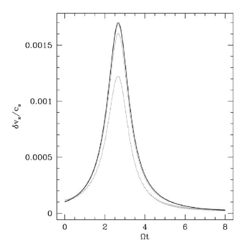
Figure 5.1: Evolution of the radial velocity amplitude for a vortical shwave. The heavy line is the analytic result, and the light lines are numerical results with (in order of increasing accuracy) $N_{x}=N_{y}=32,64,128$ and $256$.

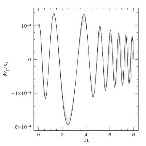
Figure 5.2: Evolution of the azimuthal velocity amplitude for a nonvortical shwave. The heavy line is the analytic result, and the light lines are numerical results with (in order of increasing accuracy) $N_{x}=N_{y}=32,64,128$ and $256$.

are the same as those in the fiducial run, except that $L=0.5H$ for the vortical-shwave evolution since $k_{y}H\gg 1$ is required to prevent mixing between vortical and non-vortical shwaves near $\tau=0$. The shwaves are well resolved until the radial wavelength $\lambda_{x}=4\times\Delta x$, and the code is capable of tracking both potential-vorticity and compressive perturbations with high accuracy.

Without a specific model for the process that is injecting the vorticity, it is difficult to settle on a particular set of initial conditions, or to know how these initial conditions ought to vary when the size of the box is allowed to vary. Our choice of initial conditions is therefore somewhat arbitrary. We use a set of initial (incompressive) velocity perturbations drawn from a Gaussian random field. The amplitude of the perturbations is characterized by $\sigma={\langle}|\delta\mbox{\boldmath$v$}|^{2}{\rangle}^{1/2}$. The power spectrum is appropriate for two dimensional Kolmogorov turbulence, $|\delta\mbox{\boldmath$v$}|^{2}\sim k^{-8/3}$, with cutoffs at $k_{min}=(1/2)(2\pi/H)$ and $k_{max}=32k_{min}$. The surface density is not perturbed. These initial conditions correspond to a set of purely vortical perturbations.

5.4 Results

The evolution of the potential vorticity in our fiducial run is shown in Figure 5.3. The snapshots are shown in lexicographic order beginning with the initial conditions, which have equal positive and negative $\delta\xi$.

One of the most remarkable features of the fiducial run evolution is the appearance of comparatively stable, long-lived vortices. These vortices have negative $\delta\xi$ and are therefore dark in Figure 5.3. Similar vortices have been seen by Godon and Livio [1999, 2000], Li et al. [2001] and Umurhan and Regev [2004]. Cross sections of one of the vortices at the end of the run are shown in Figures 5.5 and 5.5. In our models the vortices are not associated with easily identifiable features in the surface density, since the perturbed vorticity is not large enough to require, through the equilibrium condition, an order unity increase in the local pressure.

While the vortices are long-lived, they do decay. Figure 5.6 shows the evolution of the perturbed (noncircular) kinetic energy

$$E_{K}\equiv\frac{1}{2}\Sigma(\delta v_{x}^{2}+\delta v_{y}^{2})$$ (5.11)

in the fiducial run. Evidently the kinetic energy decays approximately as $t^{-1/2}$ (which is remarkable in that, if the vortices would correspond to features in luminosity that decay as $t^{-1/2}$, they could produce flicker noise; see Press 1978). Runs with half and twice the resolution decay in the same fashion, but if the resolution is reduced to $64^{2}$ the kinetic energy decays exponentially. Resolution

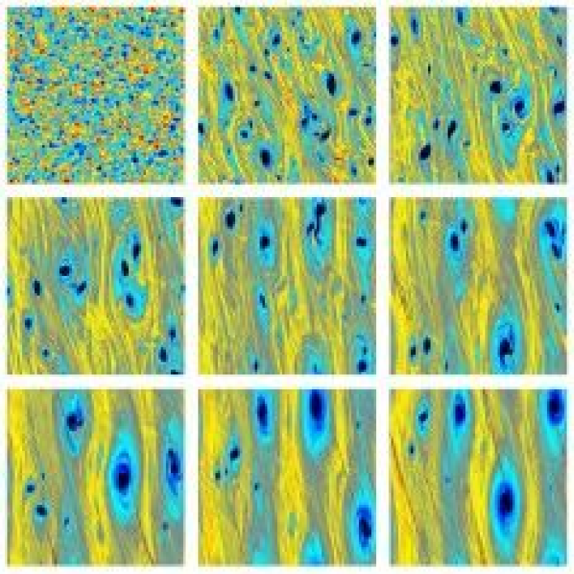
Figure 5.3: Panels show the evolution of the potential vorticity in the fiducial run. The size is $4H\times 4H$ and the numerical resolution is $1024^{2}$. The initial conditions are shown in the upper left corner, and the other frames follow in lexicographic order at intervals of $22.2\Omega^{-1}$. Dark shardes (blue and black in the color version) indicate potential vorticity smaller than $\Omega/(2\Sigma_{0})$; light shades (yellow and red in the color version) show positive potential vorticity perturbations. Evidently only the “anticyclonic” (negative potential vorticity perturbation) vortices survive. Each vortex sheds sound waves, which steepen into trailing shocks.

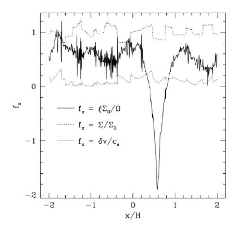
Figure 5.4: Radial slice of a vortex at the end of the fiducial run. The heavy line shows the potential vorticity, the light line shows the magnitude of the velocity and the dotted line shows the surface density.

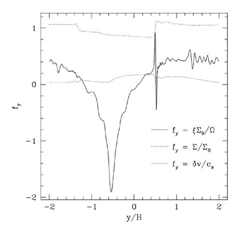
Figure 5.5: Azimuthal slice of a vortex at the end of the fiducial run. The heavy line shows the potential vorticity, the light line shows the magnitude of the velocity and the dotted line shows the surface density.

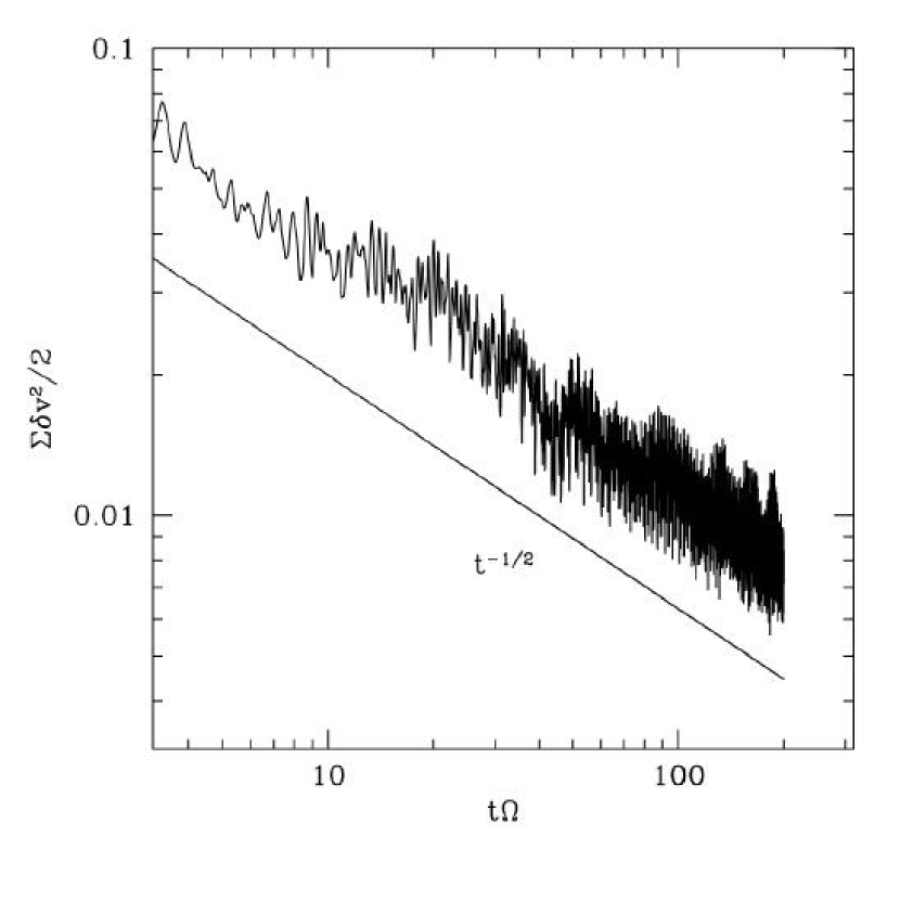
Figure 5.6: Evolution of kinetic energy in time for the fiducial run, on a log-log scale. The solid line shows a $t^{-1/2}$ decay for comparison purposes.

of at least 128 zones per scale height appears to be required.

What is even more remarkable is that the vortices are associated with an outward angular momentum flux, due to the driving of compressive motions by the vortices. Figure 5.7 shows the evolution of the dimensionless angular momentum flux

$$\alpha\equiv\frac{1}{L_{x}L_{y}\Sigma_{0}c_{s}^{2}1}\int\Sigma\delta v_{x}\delta v_{y}dxdy$$ (5.12)

for models with a variety of resolutions. The data has been boxcar smoothed over an interval $\Delta t=10\Omega^{-1}$ to make the plot readable. Again, a resolution of at least $512^{2}$ appears to be required for a converged measurement of the shear stress. For the most highly resolved models $\alpha$ evolves like the kinetic energy, $\propto t^{-1/2}$.

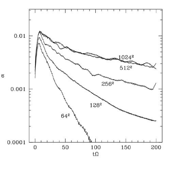
Figure 5.7: Evolution of the shear stress $\alpha$ in the fiducial run and a set of runs at lower resolutions.

Compressibility is crucial for development of the anglar momentum flux. We have demonstrated this in two ways. First, we have taken the fiducial run and decomposed the velocity field into a compressive and an incompressive part (i.e., into potential and solenoidal pieces in Fourier space) and measured the stress associated with each. For a set of snapshots taken from the last half of the fiducial run, the average total $\alpha=0.0036$; the incompressive component is $\alpha_{i}=-0.0006$; the compressive component is $\alpha_{c}=0.0032$. The remaining alpha $\alpha_{x}=0.00099$ is in cross-correlations between the incompressive and compressive pieces of the velocity field. As argued in Balbus [2000] and Balbus [2003], both incompressive trailing shwaves and incompressive turbulence tend to transport angular momentum inward, whereas trailing compressive disturbances transport angular momentum outward. Our negative (positive) value for $\alpha_{i}$ ($\alpha_{c}$) is consistent with this.

Second, we have reduced the size of the model and reduced the amplitude of the initial perturbation so that it scales with the shear velocity at the edge of the model (constant “intensity” of the turbulence, in Umurhan and Regev’s parlance). Thus the Mach number of the turbulence is reduced in proportion to the size of the box. We have compared four models, with $L=(4,2,1,0.5)H$ and $\sigma=(0.8,0.4,0.2,0.1)c_{s}$. We would expect the lower Mach number models to have smaller-amplitude compressive velocity fields and therefore, consistent with the above results, smaller angular momentum flux $\alpha$. Averaging over the second half of the simulation, we find $\alpha=(0.0031,0.0018,7.2\times 10^{-5},-9.5\times 10^{-7})$.

An additional confirmation of our overall picture can be seen in Figure 5.9, in which we show a snapshot of the velocity divergence superimposed on the potential vorticity for a medium-resolution ($256^{2}$) version of the fiducial run. The position of the shocks with respect to the vortices in this figure is consistent with our interpretation that the former are generated by the latter.

The smallest of our simulations ($L=0.5H$) is nearly incompressible, but we continue to observe $t^{-1/2}$ decay (least squares fit power law is $-0.49$) at late times. The reason that we see decay while Umurhan and Regev [2004] do not may be that: (1) the remaining compressibility in our model causes added dissipation; (2) the numerical dissipation in our code is larger than that of Umurhan and Regev [2004]; (3) the code used by Umurhan and Regev [2004] could somehow be aliasing power from trailing shwaves to leading shwaves (although they do explicitly discuss, and dismiss, this possibility).

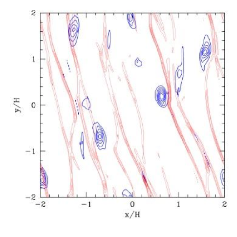
Figure 5.8: Snapshot of the velocity divergence superimposed on the potential vorticity in a medium-resolution ($256^{2}$) version of the fiducial run. The thin (red in the color version) contours indicate negative divergence and are associated with shocks. The thick (blue in the color version) contours indicate negative potential vorticity.

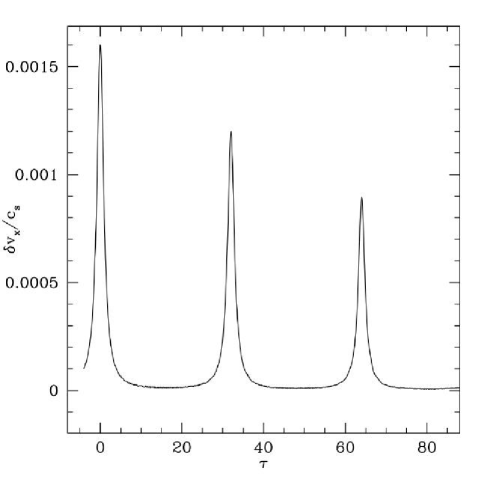
Figure 5.9: Evolution of a vortical shwave amplitude in a low-resolution ($64^{2}$) run, in units of $\tau$. The initial shwave vector ($k_{x0},k_{y}$) is ($-16\pi/L_{x},4\pi/L_{y}$), corresponding to $\tau_{0}=-4$. The interval between successive peaks (a numerical effect due to aliasing) is $\tau=N_{x}/n_{y}$, where $n_{y}=2$ is the azimuthal wavenumber.

To highlight the dangers of aliasing for our finite-difference code, in Figure 5.9 we show the evolution of a vortical shwave amplitude at low resolution ($64^{2}$), in units of $\tau$. We use the same parameters as those in our linear-theory test (Figures 5.2 and 5.2), for which the initial shwave vector corresponds to $\tau_{0}=-4$. The initially-leading shwave swings into a trailing shwave, the radial wavelength is eventually lost near the grid scale, and due to aliasing the code picks up the evolution of the shwave again as a leading shwave. Repeating this test at higher resolutions indicates that successive swings from leading to trailing occur at an interval of $\tau=N_{x}/n_{y}$, where $n_{y}=2$ is the azimuthal wavenumber of the shwave. This is equivalent to $k_{x}(t)=2\pi/\Delta x$. The decay of the successive linear solutions with time is due to numerical diffusion.

Figure 5.9 suggests that it is easier to inject power into the simulation due to aliasing rather than to remove power due to numerical diffusion. We do not believe, however, that aliasing is affecting our high-resolution results. In addition, if we assume that the flow in our simulations can be modeled as two-dimensional Kolmogorov turbulence, then $\delta v_{rms}\sim\lambda^{1/3}$, where $\delta v_{rms}$ is the rms velocity variation across a scale $\lambda$. The velocity due to the mean shear at these scales is $\delta v_{shear}\sim q\Omega\lambda$, and $\delta v_{rms}/\delta v_{shear}\sim\lambda^{-2/3}$. The velocities at the smallest scales are thus dominated by turbulence rather than by the mean shear. This conclusion is supported by the convergence of our numerical results at high resolution.

Our model contains two additional numerical parameters: the size $L$ and the initial turbulence amplitude $\sigma$. Figure 5.11 shows the evolution of $\alpha$ for several values of $\sigma$. Evidently for small enough values of $\sigma$ the $\alpha$ amplitude is reduced, but for near-sonic initial Mach numbers the $\alpha$ amplitude saturates (or at least the dependence on $\sigma$ is greatly weakened). Figure 5.11 shows the evolution for several values of $L$ but the same initial $\sigma$ and the identical initial power spectrum. For large enough $L$ the shear stress appears to be independent of $L$.

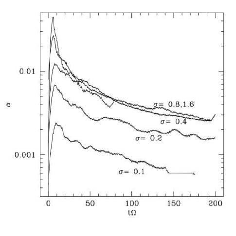
Figure 5.10: Evolution of the shear stress $\alpha$ in a set of runs at with varying initial $\sigma$. Apparently for low values of $\sigma$ the shear stress is reduced, but for initial Mach number near $1$ the stress saturates. All runs have $L=4H$.

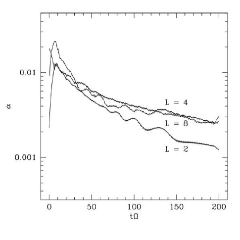
Figure 5.11: Evolution of the shear stress $\alpha$ in a set of runs at with varying initial $L$, but the same initial Mach number $\sigma$.

Finally, we have studied the autocorrelation function of the potential vorticity as a means of characterizing structure inside the flow. Figures 5.13 and 5.13 shows the autocorrelation function measured in the fiducial model and in an otherwise identical model with $L=8H$. Evidently the potential vorticity is correlated over about one-half a scale height in radius, independent of the size of the model. This supports the idea that compressive effects limit the size of the vortices, since the shear flow becomes supersonic across a vortex of size $\sim H$ [Barge and Sommeria, 1995, Li et al., 2001].

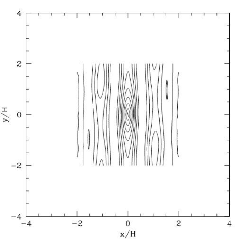
Figure 5.12: Autocorrelation function of the potential vorticity $\xi$ for the fiducial model with $L=4H$.

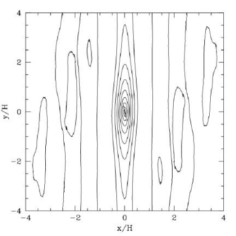
Figure 5.13: Autocorrelation function of the potential vorticity $\xi$ for a model with $L=8H$.

5.5 Conclusion

The presence of long-lived vortices in weakly-ionized disks may be an integral part of the angular momentum transport mechanism in these systems. The key result we have shown here is that compressibility of the flow is an extremely important factor in providing a significant, positively-correlated average shear stress with its associated outward transport of angular momentum. Previous results using a local model have assumed incompressible flow and either report no angular momentum transport [Umurhan and Regev, 2004] or report a value ($\alpha\sim 10^{-5}$, Barranco and Marcus 2005) that is two orders of magnitude lower than what we find when we include the effects of compressibility. Global simulations [Godon and Livio, 1999, 2000, Li et al., 2001] have a difficult time accessing the high resolution that we have shown is required for a significant shear stress due to compressibility.

Our work leaves open the key question of what happens in three dimensions. Our vortices, which have radial and azimuthal extent $\lesssim H$, are inherently three-dimensional. Three-dimensional vortices are susceptible to the elliptical instability [Kerswell, 2002] and are likely to be destroyed on a dynamical timescale. The fact that vortices persist in our two-dimensional simulations and not in the local (three-dimensional) shearing-box calculations of Balbus et al. [1996] is likely due to dimensionality. The recent numerical results of Barranco and Marcus [2005] indicate that vortices near the disk midplane are quickly destroyed, whereas vortices survive if they are a couple of scale heights away from the midplane. Strong vertical stratification away from the midplane may enforce two-dimensional flow and allow the vortices that we consider here to survive.

The initial conditions in Barranco and Marcus [2005] are analytic solutions for two-dimensional vortices that are stacked into a three-dimensional column. The stable, off-midplane vortices apparently arise due to the breaking of internal gravity waves generated by the midplane vortices before they become unstable. There is also an unidentified instability that breaks a single off-midplane vortex into several vortices. These simulations leave open the question of whether stable off-midplane vortices can be generated from a random set of initial vorticity perturbations rather than the special vortex solutions that are imposed.

Our work also leaves open the key question of what generates the initial vorticity. One possibility is that material builds up at particular radii in the disk, resulting in a global instability (e.g. Papaloizou and Pringle 1984, 1985) and a breakdown of the flow into vortices [Li et al., 2001]. Another possibility for vortex generation in variable systems is that the MHD turbulence, which likely operates during an outburst but decays as the disk cools [Gammie and Menou, 1998], leaves behind some residual vorticity. The viability of such a mechanism could be tested with non-ideal MHD simulations such as those of Fleming and Stone [2003] and Sano and Stone [2003]. Yet another possibility is that differential illumination of the disk somehow produces vorticity. Since the temperature of most circumstellar disks is controlled by stellar illumination, small variations in illumination could produce hot and cold spots in the disk that interact to produce vortices. The final possibility that we consider is the generation of vorticity via baroclinic instability, which is likely to operate in disks whose vertical stratification is close to adiabatic [Knobloch and Spruit, 1986]. The nonlinear outcome of this instability in planetary atmospheres is the formation of vortices, although it is far from clear that the same outcome will occur in disks. Finally, we note that a residual amount of vorticity can be generated from finite-amplitude compressive perturbations. We have performed a series of runs with zero initial vorticity and perturbation wavelengths on the order of the scale height, and the results are qualitatively similar to Figure 5.7 with the shear stress reduced by nearly two orders of magnitude.

Chapter 6 Summary and Outlook

Angular momentum transport is key to the evolution of accretion disks. In ionized disks, momentum transport is likely to be mediated internally by MHD turbulence generated by the MRI. Despite the success of this local shear instability in elucidating the accretion process in ionized disks, the complexity of its nonlinear outcome has raised a whole new set of questions regarding its effects upon disk evolution. The answers to most of these questions will require the use of three-dimensional numerical simulations. I discuss some of the remaining open questions in Section 6.1 and propose some simple numerical experiments that will attempt to answer them.

The mechanism driving accretion in weakly-ionized disks remains unclear. I summarize the main results of this dissertation in Section 6.2, results which mostly argue against a turbulent transport of angular momentum in these disks. I also discuss some possible directions to take in further pursuit of such a mechanism.

The fact that decades of research have not uncovered a robust turbulent transport mechanism for weakly-ionized disks raises the possibility that at least some of these disks (or portions of them) are stable and do not accrete in a steady state as the standard disk model assumes. Proposals for exploring the implications of this possibility are discussed in Section 6.3.

Finally, while modeling turbulent shear stresses as an alpha viscosity has turned out to be useful phenomenologically, representing disk turbulence as an alpha viscosity has its limitations (see Section 6.1.2), and any model results that depend upon an accurate representation of this aspect of disk physics are therefore suspect. The fundamental understanding of turbulent shear stresses in disks that has begun to emerge in recent years has opened up an exciting opportunity for developing physically-motivated disk models based upon a first-principles treatment of disk turbulence. I conclude in Section 6.4 with a discussion of proposed research along these lines.

6.1 Ionized Disks

The phenomenological approach to modeling turbulent transport in accretion disks has been challenged by the recent improved physical understanding of that transport in ionized disks. At the same time, there are important issues with regard to MHD turbulence and its ramifications for disk physics that must be understood before the standard disk model can be replaced with models based upon a more accurate representation of turbulent transport. This section discusses a few of these issues and proposes ways in which they can be investigated.

6.1.1 Transition from 2D to 3D MHD Turbulence

An important assumption underlying standard disk theory is that the global and local disk scales are well separated; small-scale turbulence is assumed to average to a smoothly-varying flow on large scales. The validity of this assumption can be tested by measuring the power spectrum of MHD turbulence in a series of three-dimensional shearing-box simulations with horizontal scales much larger than the vertical scale, looking for a transition between two-dimensional and three-dimensional behavior. If there is a transition at some characteristic scale, presumably on the order of the disk scale height, this will confirm the standard picture as well as provide a guide for the scales at which the assumptions of standard disk theory can be appropriately applied in global models. If there is no transition to smoothly-varying two-dimensional flow, much of standard disk theory is invalid.

6.1.2 Dynamics of MRI Turbulent Stresses

Turbulence is an extremely complex phenomenon, and the standard approach of modeling it as a viscosity is clearly oversimplified. For example, there are key dynamical properties of MHD turbulence, such as the elastic properties that produce magnetic tension [Ogilvie and Proctor, 2003], that cannot be modeled with a viscosity [McKinney and Gammie, 2002]. In addition, the standard disk model assumes that the turbulent shear stress is isotropic, whereas MHD turbulence is inherently anisotropic. Any model results that depend upon an accurate representation of the turbulent shear stress are therefore suspect. Ogilvie [2003] has developed an analytic model for MHD turbulent stresses consisting of evolution equations for the turbulent stress tensor. Such a model could provide the basis for more realistic analytic and numerical studies of accretion disks, as well as be useful for global disk simulations since it would allow one to represent the underlying turbulence accurately over long time scales without having to resolve the small-scale structure. I will attempt to test this model against local numerical simulations of MHD turbulence and seek to constrain the values of its free parameters.

6.1.3 Interaction of Waves with Turbulence

Another key assumption underlying many disk studies is that waves will propagate through turbulence relatively unhindered. For example, models that have been developed to explain quasi-periodic oscillations (QPOs) in binary systems often invoke characteristic oscillations of the accretion disk as the source of the QPOs [Wagoner et al., 2001]. The implicit assumption in these models is that the disk oscillations are negligibly affected by the disk turbulence. As another example, analytic studies of warped accretion disks [Papaloizou and Pringle, 1983, Papaloizou and Lin, 1995] have shown that warps will propagate as non-dispersive waves if the turbulence in the disk is sufficiently small. The turbulence in these studies is modeled as a shear viscosity, but it is not clear how the turbulence will interact with warp propagation self-consistently. As a final example, the standard disk model assumes that thermal energy is both generated and radiated locally, which results in a temperature dependence with radius that is not always observed [Robinson et al., 1999]. An alternative to this local dissipation process is a global process whereby waves are excited at one point in the disk and carry energy and angular momentum to another point in the disk before dissipating [Adams et al., 1988]. Again, wave propagation through the disk is assumed to proceed unhindered by the turbulence.

The general problem of the interaction of waves with turbulence has been well-studied analytically, particularly in the context of solar oscillations (Goldreich and Kumar 1988, 1990; see also Farmer and Goldreich 2004), but numerical studies along these lines are less advanced (see Torkelsson et al. 2000 for one example). I will seek to further our understanding in this area by investigating, via numerical experiments, the effect of turbulence on waves propagating through a disk. A wave or superposition of wave modes calculated from linear theory will be inserted into a magnetized turbulent numerical model, and the subsequent evolution will be compared with the linear theory results. The outcome of these experiments will determine whether or not the neglect of wave-turbulence interactions is valid. If there is significant interaction, these experiments may provide a means for developing a predictive theory of wave propagation in turbulent disks.

6.2 Weakly-Ionized Disks

The prospects of discovering a turbulent transport mechanism in weakly-ionized accretion disks appear to be dim. Since proving stability is much more difficult than demonstrating instability, however, the search for such a transport mechanism continues. The most promising mechanism based upon the work discussed in this dissertation is the driving of compressive motions by vortices, but even this faces serious difficulties due to the decaying angular momentum flux and the potential for the vortices to be unstable in three dimensions. It would be useful to redo in three dimensions the simulations discussed in Chapter 5, to determine the rate at which the vortices become unstable and the nonlinear outcome of such an instability. Testing some of the vorticity-generation mechanisms discussed in §5.5 is also a necessary next step in understanding the relevance of this overall picture for driving accretion in weakly-ionized disks.

The possibility of a bypass transition to turbulence due to the transient amplification of linear disturbances followed by a nonlinear feedback from trailing shwaves (shearing waves) into leading shwaves has not been fully explored. The effects of aliasing shown in Figure 4.15 clearly demonstrate that such a feedback mechanism can result in the overall growth of linear disturbances into the nonlinear regime. While the feedback in Figure 4.15 is entirely numerical, the high-resolution requirements for tracking these shwaves (as can be seen in Figure 4.2) implies that the nonlinear outcome of transient amplification has not been tested at the resolutions we employ for the runs discussed in Chapter 4.

Vanneste et al. [1998] calculated three-shwave interactions in the unstratified (incompressible) shearing sheet and found that there is feedback from trailing shwaves into leading shwaves for a small subset of initial shwave vectors. It would be of interest to revisit this calculation in the stratified shearing sheet. One key difference between the stratified and unstratified shearing-sheet models is that in the latter case all linear perturbations decay after their transient growth, whereas in the former case the density perturbation does not decay. This implies that quasilinear interactions are more likely to take place. A comparison of Figures 5.9 and 4.15 indicates that feedback due to aliasing in the unstratified sheet does not result in any overall growth, whereas feedback in the stratified sheet does.

6.3 Layered Disks

A more fruitful line of research may be to simply assume that a weakly-ionized flow is stable. Accretion in that case could proceed in surface layers that are ionized by non-thermal radiative processes, with the mid-plane of the disk remaining inactive (see Figure 6.1 and Gammie 1996). One of the few numerical studies of layered accretion has shown that there may be some wave transport from the active, MHD-turbulent zone to the inactive zone [Fleming and Stone, 2003]. This work could be expanded upon with a more realistic treatment of the vertical structure and vertical boundary conditions, as well as a closer inspection of the stresses in the inactive zone, including an investigation of their dependence on simulation parameters. Understanding these processes would be useful for developing more sophisticated models of layered disks.

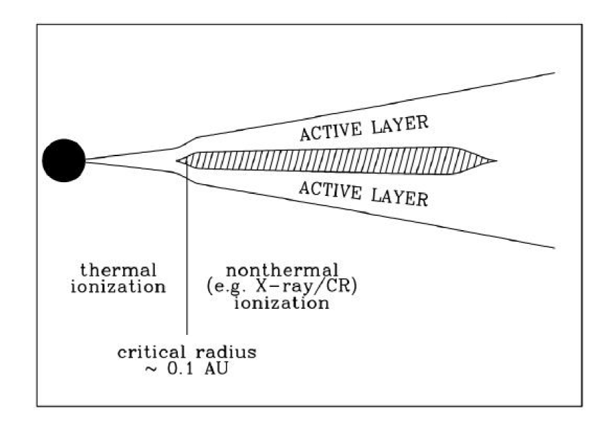
Figure 6.1: Ionization structure of YSO disks. The inner disk is coupled to the field via thermal ionization. At larger radii the surface layers are coupled but the midplane (hashed) is inactive. At still larger radii the density is lower and nonthermal ionization provides effective coupling throughout the disk.

In addition, since the dynamics of the dust layer in protoplanetary disks (disks which are likely to be weakly-ionized) have important implications for understanding planet formation, a useful and natural extension to the research proposed here is to incorporate gas-dust interactions in some of my calculations. The effects of turbulence and wave transport on the dust layer could be investigated by including dust particles of various sizes in numerical simulations similar to those described in Section 6.1.3. In addition, interactions could be calculated self-consistently by incorporating dust dynamics into layered disk models using a two-fluid approach.

6.4 Advanced Physical Disk Models

The majority of analytic [Shakura and Sunyaev, 1973, Lynden-Bell and Pringle, 1974, Pringle, 1981, Hartmann, 1998] and numerical [Igumenshchev and Abramowicz, 1999, Stone et al., 1999, Igumenshchev and Abramowicz, 2000, Igumenshchev et al., 2000, McKinney and Gammie, 2002] accretion-disk studies incorporate the assumption of an alpha viscosity to model disk turbulence. As discussed in §6.1.2, such an assumption has its shortcomings. A fundamental understanding of MHD turbulent stresses can be used to develop advanced disk models that will enhance our ability to explain observations of accretion systems.

Numerical models that rely on an alpha viscosity could be improved upon by incorporating a more sophisticated model for the turbulent stresses based upon simulations and theoretical studies of turbulence, such as those described in Section 6.1.2. In addition to being useful for modeling accretion systems, these models would provide a more reliable bridge between local and global MHD simulations and possibly be a means for understanding the complex results of global MHD simulations at a more fundamental level.

Analytic models that incorporate more sophisticated turbulent-stress modeling could also be developed in an effort to improve upon the standard disk model. In addition, there may be key analytic results that need to be revisited with an enhanced understanding of turbulent stresses, such as the work on wave propagation in warped disks discussed in §6.1.3 [Papaloizou and Pringle, 1983, Papaloizou and Lin, 1995]. All of these proposals represent potential progress towards a first-principles understanding and modeling of accretion-disk systems.

Appendix A The Boussinesq Approximation

We demonstrate here that the Boussinesq approximation to the linear perturbation equations is formally equivalent to a short-wavelength, low-frequency limit of the full set of linear equations. We perform the demonstration for the stratified shearing-sheet model since the standard shearing sheet is recovered in the limit of zero stratification.

Combining equations (3.45) through (3.49) into a single equation for $\delta v_{x}$ yields the following differential equation, fourth-order in time:

$$F_{4}\delta v_{x}^{(4)}+F_{3}\delta v_{x}^{(3)}+F_{2}\delta v_{x}^{(2)}+F_{1}\delta v_{x}^{(1)}+F_{0}\delta v_{x}=0,$$ (A.1)

where

$$F_{4}=\tilde{k}_{x}^{2}\left[(k_{y}^{2}+k_{z}^{2})\left(1-\frac{i}{\tilde{k}_{x}L_{P}}\right)^{2}+k_{y}^{2}\frac{2({\tilde{q}}+1)({\tilde{q}}+2)}{\tilde{k}_{x}^{2}H^{2}}\right],$$ (A.2)

$$F_{3}=-2{\tilde{q}}\Omega\tilde{k}_{x}k_{y}(k_{y}^{2}+k_{z}^{2})\left(1+\frac{i}{\tilde{k}_{x}L_{P}}\right),$$ (A.3)

$$F_{2}=c_{s}^{2}\tilde{k}_{x}^{2}\left[\tilde{k}_{x}^{2}\left(1+\frac{1}{\tilde{k}_{x}^{2}L_{P}^{2}}+\frac{N_{x}^{2}+\tilde{\kappa}^{2}}{\tilde{k}_{x}^{2}H^{2}}\right)\left\{(k_{y}^{2}+k_{z}^{2})\left(1-\frac{i}{\tilde{k}_{x}L_{P}}\right)^{2}+k_{y}^{2}\frac{2({\tilde{q}}+1)({\tilde{q}}+2)}{\tilde{k}_{x}^{2}H^{2}}\right\}\,+\right.$$

$$\left.(k_{y}^{2}+k_{z}^{2})\left\{(k_{y}^{2}+k_{z}^{2})\left(1-\frac{i}{\tilde{k}_{x}L_{P}}\right)^{2}+k_{y}^{2}\frac{2({\tilde{q}}+1)(3{\tilde{q}}+2)}{\tilde{k}_{x}^{2}H^{2}}\right\}\right],$$ (A.4)

$$F_{1}=4{\tilde{q}}\Omega c_{s}^{2}k_{y}\tilde{k}_{x}^{3}\left[(k_{y}^{2}+k_{z}^{2})\left(1+\frac{i}{\tilde{k}_{x}L_{P}}\right)\left\{1+\frac{i(3{\tilde{q}}-2)}{2{\tilde{q}}\tilde{k}_{x}L_{P}}+\frac{\tilde{\kappa}^{2}}{4{\tilde{q}}\tilde{k}_{x}^{2}L_{P}^{2}}-\frac{N_{x}^{2}+\tilde{\kappa}^{2}}{2\tilde{k}_{x}^{2}H^{2}}\right\}\,+\right.$$

$$\left.3k_{y}^{2}\frac{({\tilde{q}}+1)({\tilde{q}}+2)}{\tilde{k}_{x}^{2}H^{2}}\left(1-\frac{2i}{3{\tilde{q}}\tilde{k}_{x}L_{P}}\right)\right],$$ (A.5)

$$F_{0}=c_{s}^{2}\tilde{k}_{x}^{2}\left[k_{y}^{2}(N_{x}^{2}+2{\tilde{q}}^{2}\Omega^{2})+k_{z}^{2}(N_{x}^{2}+\tilde{\kappa}^{2})\right]\left[(k_{y}^{2}+k_{z}^{2})\left(1-\frac{i}{\tilde{k}_{x}L_{P}}\right)^{2}+k_{y}^{2}\frac{2({\tilde{q}}+1)(3{\tilde{q}}+2)}{\tilde{k}_{x}^{2}H^{2}}\right].$$ (A.6)

The above expressions have been written to make the short-wavelength limit more apparent: all but the leading-order terms in brackets are proportional to factors of $(\tilde{k}_{x}L_{P})^{-1}$ or $(\tilde{k}_{x}H)^{-1}$. Notice also that since one expects $H/L_{P}\ll 1$ for Keplerian disks with modest radial gradients,

$$\frac{1}{\tilde{k}_{x}L_{P}}=\frac{1}{k_{y}H\tilde{\tau}}\frac{H}{L_{P}}\ll\frac{1}{k_{y}H\tilde{\tau}},$$ (A.7)

(for $\tilde{\tau}\neq 0$) and therefore the short-wavelength limit is sufficient. One needs to be careful in taking this limit, however, since $\tilde{k}_{x}=k_{y}\tilde{\tau}$ goes through zero as a shwave goes from leading to trailing. The approximation is rigorously valid only for $\tilde{\tau}\neq 0$, but we have numerically integrated the full set of linear equations (equations (3.45) through (3.49) with $k_{z}=0$) and found good agreement with the Boussinesq solutions described in §4.3 for all $\tilde{\tau}$ at sufficiently short wavelengths.

With these assumptions in mind, to leading order in $(Hk_{y})^{-1}$ equation (A.1) becomes

$$\tilde{k}_{x}\delta v_{x}^{(4)}-2{\tilde{q}}\Omega k_{y}\delta v_{x}^{(3)}+c_{s}^{2}\tilde{k}_{x}\tilde{k}^{2}\delta v_{x}^{(2)}+4{\tilde{q}}\Omega c_{s}^{2}\tilde{k}_{x}^{2}k_{y}\delta v_{x}^{(1)}\,+$$

$$c_{s}^{2}\tilde{k}_{x}\left[k_{y}^{2}(N_{x}^{2}+2{\tilde{q}}^{2}\Omega^{2})+k_{z}^{2}(N_{x}^{2}+\tilde{\kappa}^{2})\right]\delta v_{x}=0.$$ (A.8)

If we assume $\partial_{t}\ll c_{s}k_{y}$, the two highest-order time derivatives are of lower order and can be neglected (thereby eliminating the compressive shwaves) and we have

$$\tilde{k}^{2}\ddot{\delta v_{x}}+4{\tilde{q}}\Omega\tilde{k}_{x}k_{y}\dot{\delta v_{x}}\left[k_{y}^{2}(N_{x}^{2}+2{\tilde{q}}^{2}\Omega^{2})+k_{z}^{2}(N_{x}^{2}+\tilde{\kappa}^{2})\right]\delta v_{x}=0.$$ (A.9)

This is equivalent to equation (3.56).

Notice also that the assumption $\partial_{t}\sim O(c_{s}k_{y})$ applied to equation (A) yields

$$\delta v_{x}^{(4)}+c_{s}^{2}\tilde{k}^{2}\delta v_{x}^{(2)}=0$$ (A.10)

to leading order in $(Hk_{y})^{-1}$. This equation is of the same form as the short-wavelength limit of equation (3.16) for the compressive shwaves in the unstratified shearing sheet, confirming our claim that short-wavelength compressive shwaves are unchanged at leading order by stratification.

Appendix B Curriculum Vitae

Bryan Mark Johnson

ADDRESS

Loomis Laboratory of Physics

University of Illinois at Urbana-Champaign

1110 West Green Street

Urbana, IL 61801

Phone: (217) 333-2327

e-mail: bmjohnso@uiuc.edu

EDUCATION

Ph.D. in Physics, University of Illinois at Urbana-Champaign, 2005 (Advisor: Gammie).

Dissertation: Turbulent Angular Momentum Transport in Weakly-Ionized Accretion Disks.

B.S. Electrical Engineering, LeTourneau University, 1996 (Advisor: Knoop).

Senior thesis: System Measurement with White Noise.

EXPERIENCE

Teaching Assistant, University of Illinois at Urbana-Champaign, 2000-2002.

Systems Integration Engineer, Northrop Grumman Corporation, 1997-2000.

HONORS AND AWARDS

Drickamer Research Fellowship, University of Illinois, 2004: to recognize a graduate student who has demonstrated significant ability in research, the most prestigious prize given by the Department of Physics to a graduate student.

R.G. LeTourneau Award for Outstanding Senior Engineering Student, LeTourneau University, 1996.

Gold Key Honor Society, LeTourneau University, 1996: represents the highest honor given by LeTourneau University to outstanding senior students.

Dean’s Scholarship, LeTourneau University, 1994.

Northrop Corporation Engineering Scholarship, Harper College, 1993.

Square D Engineering Scholarship, Harper College, 1992.

President’s Scholarship, Crown College, 1990.

References

- Abramowitz and Stegun [1972] M. Abramowitz and I. A. Stegun. Handbook of Mathematical Functions. Handbook of Mathematical Functions, New York: Dover, 1972, 1972.
- Adams and Lin [1993] F. C. Adams and D. N. C. Lin. Transport processes and the evolution of disks. In Protostars and Planets III, pages 721–748, 1993.
- Adams et al. [1988] F. C. Adams, F. H. Shu, and C. J. Lada. The disks of T Tauri stars with flat infrared spectra. ApJ, 326:865–883, March 1988.
- Afshordi et al. [2004] N. Afshordi, B. Mukhopadhyay, and R. Narayan. Bypass to Turbulence in Hydrodynamic Accretion: Lagrangian Analysis of Energy Growth. ArXiv Astrophysics e-prints, December 2004.
- Arlt and Rüdiger [2001] R. Arlt and G. Rüdiger. Global accretion disk simulations of magneto-rotational instability. A&A, 374:1035–1048, August 2001.
- Armitage [1998] P. J. Armitage. Turbulence and Angular Momentum Transport in Global Accretion Disk Simulation. ApJ, 501:L189, July 1998.
- Baggett and Trefethen [1997] J. S. Baggett and L. N. Trefethen. Low-dimensional models of subcritical transition to turbulence. Physics of Fluids, 9:1043–1053, April 1997.
- Balbus [1988] S. A. Balbus. Local interstellar gasdynamical stability and substructure in spiral arms. ApJ, 324:60–74, January 1988.
- Balbus [2000] S. A. Balbus. Stability, Instability, and “Backward” Transport in Stratified Fluids. ApJ, 534:420–427, May 2000.
- Balbus [2003] S. A. Balbus. Enhanced Angular Momentum Transport in Accretion Disks. ARA&A, 41:555–597, 2003.
- Balbus [2004] S. A. Balbus. Nonlinear Scale Invariance in Local Disk Flows. ArXiv Astrophysics e-prints, August 2004.
- Balbus and Hawley [1991] S. A. Balbus and J. F. Hawley. A powerful local shear instability in weakly magnetized disks. I - Linear analysis. II - Nonlinear evolution. ApJ, 376:214–233, July 1991.
- Balbus and Hawley [1992] S. A. Balbus and J. F. Hawley. Is the Oort A-value a universal growth rate limit for accretion disk shear instabilities? ApJ, 392:662–666, June 1992.
- Balbus and Hawley [1998] S. A. Balbus and J. F. Hawley. Instability, turbulence, and enhanced transport in accretion disks. Reviews of Modern Physics, 70:1–53, January 1998.
- Balbus et al. [1996] S. A. Balbus, J. F. Hawley, and J. M. Stone. Nonlinear Stability, Hydrodynamical Turbulence, and Transport in Disks. ApJ, 467:76, August 1996.
- Balbus and Terquem [2001] S. A. Balbus and C. Terquem. Linear Analysis of the Hall Effect in Protostellar Disks. ApJ, 552:235–247, May 2001.
- Baptista [2004] R. Baptista. What can we learn from accretion disc eclipse mapping experiments? Astronomische Nachrichten, 325:181–184, 2004.
- Baptista et al. [1998] R. Baptista, K. Horne, R. A. Wade, I. Hubeny, K. S. Long, and R. G. M. Rutten. HST spatially resolved spectra of the accretion disc and gas stream of the nova-like variable UX Ursae Majoris. MNRAS, 298:1079–1091, August 1998.
- Barge and Sommeria [1995] P. Barge and J. Sommeria. Did planet formation begin inside persistent gaseous vortices? A&A, 295:L1–L4, March 1995.
- Barranco and Marcus [2005] J. A. Barranco and P. S. Marcus. Three-Dimensional Vortices in Stratified Protoplanetary Disks. ArXiv Astrophysics e-prints, January 2005.
- Bayly et al. [1988] B. J. Bayly, S. A. Orszag, and T. Herbert. Instability mechanisms in shear-flow transition. Annual Review of Fluid Mechanics, 20:359–391, 1988.
- Bell and Lin [1994] K. R. Bell and D. N. C. Lin. Using FU Orionis outbursts to constrain self-regulated protostellar disk models. ApJ, 427:987–1004, June 1994.
- Binney and Tremaine [1987] J. Binney and S. Tremaine. Galactic dynamics. Princeton, NJ, Princeton University Press, 1987, 747 p., 1987.
- Blaes [1987] O. M. Blaes. Stabilization of non-axisymmetric instabilities in a rotating flow by accretion on to a central black hole. MNRAS, 227:975–992, August 1987.
- Blaes and Balbus [1994] O. M. Blaes and S. A. Balbus. Local shear instabilities in weakly ionized, weakly magnetized disks. ApJ, 421:163–177, January 1994.
- Blaes and Hawley [1988] O. M. Blaes and J. F. Hawley. Nonaxisymmetric disk instabilities - A linear and nonlinear synthesis. ApJ, 326:277–291, March 1988.
- Blandford and Payne [1982] R. D. Blandford and D. G. Payne. Hydromagnetic flows from accretion discs and the production of radio jets. MNRAS, 199:883–903, June 1982.
- Boss [1997] A. P. Boss. Giant planet formation by gravitational instability. Science, 276:1836–1839, 1997.
- Boss [1998] A. P. Boss. Evolution of the Solar Nebula. IV. Giant Gaseous Protoplanet Formation. ApJ, 503:923, August 1998.
- Boss [2002] A. P. Boss. Evolution of the Solar Nebula. V. Disk Instabilities with Varied Thermodynamics. ApJ, 576:462–472, September 2002.
- Burrows et al. [1996] C. J. Burrows, K. R. Stapelfeldt, A. M. Watson, J. E. Krist, G. E. Ballester, J. T. Clarke, D. Crisp, J. S. Gallagher, R. E. Griffiths, J. J. Hester, J. G. Hoessel, J. A. Holtzman, J. R. Mould, P. A. Scowen, J. T. Trauger, and J. A. Westphal. Hubble Space Telescope Observations of the Disk and Jet of HH 30. ApJ, 473:437–+, December 1996.
- Cabot [1984] W. Cabot. The nonaxisymmetric baroclinic instability in thin accretion disks. ApJ, 277:806–812, February 1984.
- Cabot [1996] W. Cabot. Numerical Simulations of Circumstellar Disk Convection. ApJ, 465:874, July 1996.
- Cameron [1978] A. G. W. Cameron. Physics of the primitive solar accretion disk. Moon and Planets, 18:5–40, February 1978.
- Cassen [1993] P. Cassen. Why convective heat transport in the solar nebula was inefficient. In Lunar and Planetary Institute Conference Abstracts, pages 261–262, 1993.
- Chagelishvili et al. [1997] G. D. Chagelishvili, A. G. Tevzadze, G. Bodo, and S. S. Moiseev. Linear Mechanism of Wave Emergence from Vortices in Smooth Shear Flows. Physical Review Letters, 79:3178–3181, October 1997.
- Chagelishvili et al. [2003] G. D. Chagelishvili, J.-P. Zahn, A. G. Tevzadze, and J. G. Lominadze. On hydrodynamic shear turbulence in Keplerian disks: Via transient growth to bypass transition. A&A, 402:401–407, May 2003.
- Chimonas [1970] G. Chimonas. The extension of the Miles-Howard theorem to compressible fluids. J. Fluid Mech., 43:833–836, 1970.
- Desch [2004] S. J. Desch. Linear Analysis of the Magnetorotational Instability, Including Ambipolar Diffusion, with Application to Protoplanetary Disks. ApJ, 608:509–525, June 2004.
- Drazin and Reid [1981] P. G. Drazin and W. H. Reid. Hydrodynamic stability. NASA STI/Recon Technical Report A, 82:17950, 1981.
- Dubrulle [1993] B. Dubrulle. Differential rotation as a source of angular momentum transfer in the solar nebula. Icarus, 106:59, November 1993.
- Dubrulle and Knobloch [1992] B. Dubrulle and E. Knobloch. On the local stability of accretion disks. A&A, 256:673–678, March 1992.
- Dubrulle and Knobloch [1993] B. Dubrulle and E. Knobloch. On instabilities in magnetized accretion disks. A&A, 274:667, July 1993.
- Durisen et al. [2001] R. H. Durisen, A. C. Mejia, B. K. Pickett, and T. W. Hartquist. Gravitational Instabilities in the Disks of Massive Protostars as an Explanation for Linear Distributions of Methanol Masers. ApJ, 563:L157–L160, December 2001.
- Eliassen et al. [1953] A. Eliassen, E. Høiland, and E. Riis. Two-Dimensional Perturbation of a Flow with Constant Shear of a Stratified Fluid. Institute for Weather and Climate Research, Nowegian Academy of Sciences and Letters, Publ. no. 1, 1, 1953.
- Farmer and Goldreich [2004] A. J. Farmer and P. Goldreich. Wave Damping by Magnetohydrodynamic Turbulence and Its Effect on Cosmic-Ray Propagation in the Interstellar Medium. ApJ, 604:671–674, April 2004.
- Farrell and Ioannou [1993] B. F. Farrell and P. J. Ioannou. Optimal excitation of three-dimensional perturbations in viscous constant shear flow. Physics of Fluids, 5:1390–1400, June 1993.
- Fleming and Stone [2003] T. Fleming and J. M. Stone. Local Magnetohydrodynamic Models of Layered Accretion Disks. ApJ, 585:908–920, March 2003.
- Fleming et al. [2000] T. P. Fleming, J. M. Stone, and J. F. Hawley. The Effect of Resistivity on the Nonlinear Stage of the Magnetorotational Instability in Accretion Disks. ApJ, 530:464–477, February 2000.
- Frank et al. [1981] J. Frank, A. R. King, M. R. Sherrington, R. F. Jameson, and D. J. Axon. Infrared and optical light curves of UX Ursae Majoris and U Geminorum. MNRAS, 195:505–516, May 1981.
- Fromang et al. [2002] S. Fromang, C. Terquem, and S. A. Balbus. The ionization fraction in models of protoplanetary discs. MNRAS, 329:18–28, January 2002.
- Gammie [1996] C. F. Gammie. Layered Accretion in T Tauri Disks. ApJ, 457:355, January 1996.
- Gammie [1999] C. F. Gammie. Instabilities in Circumstellar Discs. In ASP Conf. Ser. 160: Astrophysical Discs - an EC Summer School, page 122, April 1999.
- Gammie [2001] C. F. Gammie. Nonlinear Outcome of Gravitational Instability in Cooling, Gaseous Disks. ApJ, 553:174–183, May 2001.
- Gammie and Menou [1998] C. F. Gammie and K. Menou. On the Origin of Episodic Accretion in Dwarf Novae. ApJ, 492:L75, January 1998.
- Gammie et al. [1999] C. F. Gammie, R. Narayan, and R. Blandford. What Is the Accretion Rate in NGC 4258? ApJ, 516:177–186, May 1999.
- Garaud and Lin [2004] P. Garaud and D. N. C. Lin. On the Evolution and Stability of a Protoplanetary Disk Dust Layer. ApJ, 608:1050–1075, June 2004.