A Model for Patchy Reconnection in Three Dimensions

Abstract

We show, theoretically and via MHD simulations, how a short burst of reconnection localized in three dimensions on a one-dimensional current sheet creates a pair of reconnected flux tubes. We focus on the post-reconnection evolution of these flux tubes, studying their velocities and shapes. We find that slow-mode shocks propagate along these reconnected flux tubes, releasing magnetic energy as in steady-state Petschek reconnection. The geometry of these three-dimensional shocks, however, differs dramatically from the classical two-dimensional geometry. They propagate along the flux tube legs in four isolated fronts, whereas in the two-dimensional Petschek model, they form a continuous, stationary pair of V-shaped fronts.

We find that the cross sections of these reconnected flux tubes appear as teardrop shaped bundles of flux propagating away from the reconnection site. Based on this, we argue that the descending coronal voids seen by Yohkoh SXT, LASCO, and TRACE are reconnected flux tubes descending from a flare site in the high corona, for example after a coronal mass ejection. In this model, these flux tubes would then settle into equilibrium in the low corona, forming an arcade of post-flare coronal loops.

1 INTRODUCTION

Coronal mass ejections (CMEs), sudden eruptions of coronal plasma and magnetic field into the interplanetary medium, are one of the most dynamic phenomena in the solar corona. When these ejections collide with the Earth’s magnetosphere, they can have dramatic effects on the Earth’s space weather. Even if they miss the Earth, these CMEs are an important driver of space weather through the magnetic reconnection and flaring that is driven in the corona in their wake. Particles accelerated during the flares associated with CMEs can damage satellites and create radiation hazards for astronauts, and significant EUV and X-ray emission is generated by the coronal plasma heated by these flares.

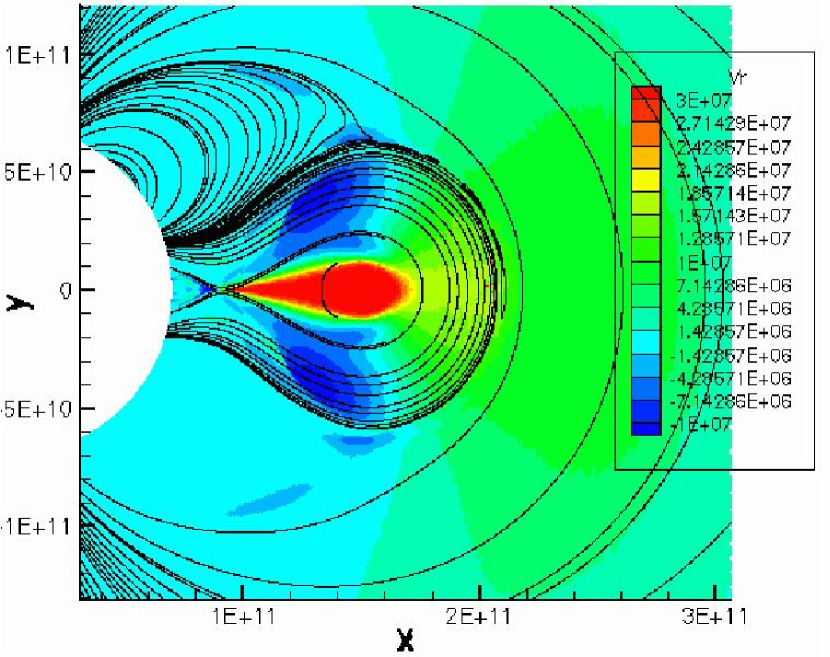
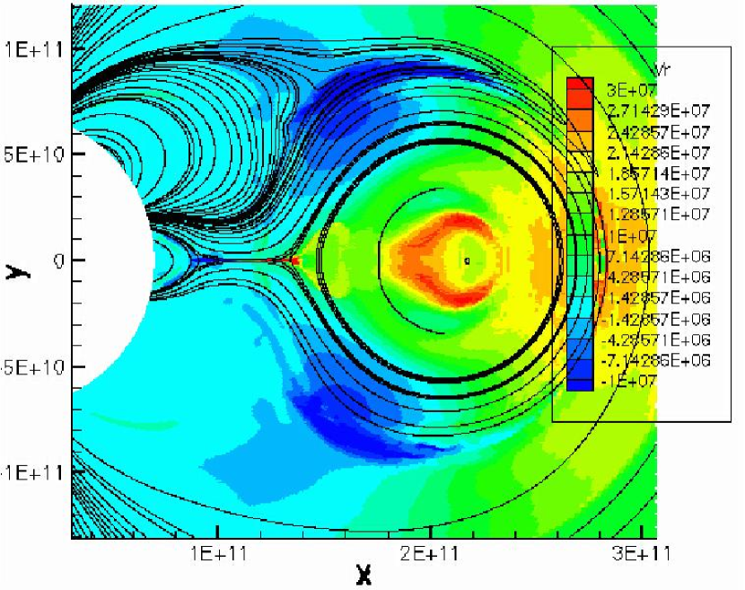
Figure 1: Snapshots from a two dimensional MHD simulation of a coronal mass ejection, showing the geometry of the fields during eruption. The field bows out from the low corona in the left panel, erupting from the solar atmosphere. Once the eruption is fully developed, the field starts to pinch off and reconnect on the back side of the CME, as shown in the right hand panel. The reconnected fields on the right hand side of this newly formed current sheet spring up to the CME, while those on the left side spring down into the corona to form arcade loops. From MacNeice et al., (2004).

Theories for the cause and form of CMEs vary (see, e.g., reviews by Forbes,, 2000; Klimchuk,, 2001; Low,, 2001; Lin et al.,, 2003), but in all cases the CME is a magnetically dominated structure, and magnetic energy release plays a prominent role in its eruption. In these models, magnetic field lines, carrying coronal plasma with them, bow out from the low corona to form the CME, as in the simulation shown in Figure 1 (MacNeice et al.,, 2004).

A critical step of the process is the reconnection of magnetic field in the wake of the CME. Prior to such reconnection the inward and outward directed field lines in the two legs of the CME are pinched together to form a current sheet. When the field reconnects across this sheet, as shown in the right hand panel of Figure 1, the CME is untethered from the Sun while the field on the sunward end of the sheet forms post-eruption coronal loops. As more of the field reconnects, these post-eruption coronal loops build up on top of each other to higher and higher altitudes, and the footpoints of each new set of loops are more and more widely separated. This classic two-dimensional flare model (see, e.g., Carmichael,, 1964; Sturrock,, 1966; Hirayama,, 1974; Kopp & Pneuman,, 1976) explains both the appearance of progressively higher coronal loops in a post-CME reconnection event, and the appearance of progressively more widely separated H$\alpha$ footpoints of the loops.

The basic process of reconnection across a current sheet was first studied in two-dimensional, steady-state models which assumed uniform resistivity (Sweet,, 1958; Parker,, 1957). The reconnection rates in such models were usually too low to explain the fairly rapid development observed in CMEs (see, e.g., Biskamp,, 1986). A faster reconnection regime was proposed first by Petschek, (1964); it was distinguished by a very small diffusion region with four slow-mode shocks linked to it. It turns out such a structure is inconsistent with spatially uniform diffusion (Kulsrud,, 2001), but occurs naturally whenever the magnetic diffusion coefficient, or any other non-ideal field line transport mechanism, is locally enhanced. This explains the notable successes of a number of modified reconnection models whereby fast reconnection can occur across a current sheet provided it is spatially localized, as by a locally enhanced resistivity (Ugai & Tsuda,, 1977; Scholer & Roth,, 1987; Erkaev et al.,, 2000). The degree of enhancement is not nearly as important as its localization (Biskamp & Schwarz,, 2001).

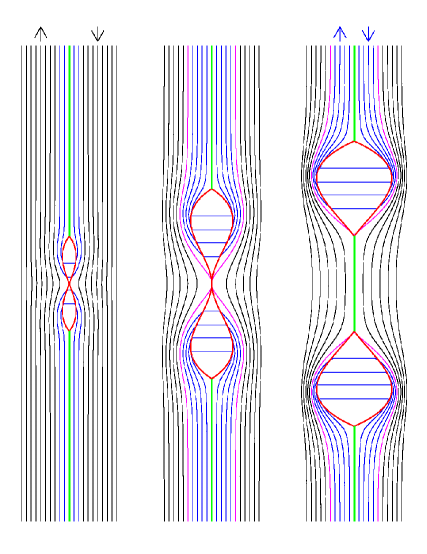
Figure 2: Theoretical field configuration for a burst of reconnection in 2D. The red lines show the slow shock fronts, the green lines show the current sheet, the blue lines are reconnected field lines, the black lines are unreconnected field lines, and the pink lines are the separatrices between the two. From Longcope, (2004), after Biernat et al., (1987).

While the hypothesis of localization solves the puzzle of fast reconnection, it raises new questions about how such a small-scale phenomenon might couple to the global magnetic field, say of the CME. A partial answer was provided by investigations of two-dimensional, localized, non-steady reconnection beginning with Semenov et al., (1983) and subsequently developed by Biernat et al., (1987), Heyn & Semenov, (1996) and Nitta et al., (2001). These models postulate a localized, non-steady reconnection electric field on a pre-existing current sheet and solve for the external response. The time-dependent solution, shown in Figure 2, consists of a pair of post-reconnection loops retracting at the Alfvén speed. Some models also include a small-amplitude fast mode wave propagating radially outward, in advance of the slow-mode shocks (Semenov et al.,, 1983; Heyn & Semenov,, 1996; Nitta et al.,, 2002); others such as Biernat et al., (1987) treat this as a static disturbance to the up-stream field.

This two-dimensional model demonstrates several respects in which localized, non-steady reconnection differs from the more well-known steady-state scenario. For example, during reconnection four slow-mode shocks extend from the reconnection site as in the steady-state Petschek model, but they do not extend to infinity, as in the steady-state. Rather they close around the tips of the unreconnected flux tubes (see Fig 2). In addition, when reconnection ceases the flux-tubes continue to retract, with the teardrop-shaped slow-mode shock fronts remaining intact, and a new current sheet forming behind them. Even then, the magnetic energy of the system continues to decrease as the flux tubes retract. This means that the energy released by the reconnection (i.e., converted from magnetic to kinetic and thermal energy by the shocks) can far exceed the energy actually dissipated (converted directly to heat by the reconnection electric field). Finally, the loops continue to sweep up mass into their slow-mode shock envelope as they retract, thereby growing indefinitely through snow-plow–like effect (Semenov et al.,, 1998).

The present work is aimed at generalizing this scenario to localized, non-steady reconnection in three dimensions, which we call patchy reconnection. The objective is to characterize the effect on the global field of reconnection occurring within a small region of a pre-existing current sheet. In particular, we solve for the dynamics of the post-reconnection flux tubes once they have been created by some reconnection process. This is a question of fundamental importance in the study of magnetic reconnection, as well as a critical element in understanding CMEs.

Observational approaches have been slow to yield this understanding since post-reconnection fields are not observable immediately after the CME. Rather, only the resulting changes in the coronal configuration are observed. This is because newly forming reconnected loops only become visible in emission after most of their energy has been released and they fill up with hot plasma. This stage only occurs as the loops approach their equilibrium state in the low corona, and so both the initial reconnection and the majority of the subsequent dynamics are unobserved. Thus even truly dynamic studies such as those of Forbes & Acton, (1996) can only observe the end stage of the loop evolution. The apparent dynamics which the two-dimensional models explain so well are simply the gradual brightening of successively higher coronal loops with successively wider footpoints. These two-dimensional reconnection models can therefore only compare their predictions with observations of the final equilibrium of the magnetic field. While they have been quite successful in this endeavor, the dynamics of the reconnection and even of the loops themselves remain largely untested.

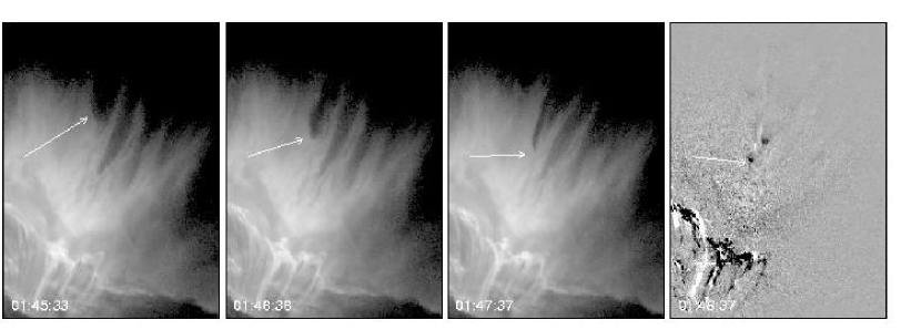
Figure 3: TRACE Images from the April 21, 2002 X flare. The first three panels show unsubtracted images from the flare. The diffuse, bright emission corresponds to high temperature plasma from the Fe XXIV 192 Å line in the TRACE 195 Å bandpass. The loop-like structures on the bottom of the arcade are loops that have cooled down to about 1 MK and are emitting in Fe XII 195 Å. The arrow points to a void that is descending through the hot plasma cloud. The final panel is a difference image between successive TRACE exposures. From Sheeley et al., (2004).

A newly observed phenomenon exhibiting genuine three-dimensional characteristics now offers a promising way to probe the coronal dynamics of reconnection: dark voids, shown in Figure 3, are observed by TRACE and Yohkoh SXT descending through the haze of 15MK post-eruption loops in the corona (see, e.g., McKenzie & Hudson,, 1999; Gallagher et al.,, 2002; Innes et al.,, 2003; Asai et al.,, 2004; Sheeley et al.,, 2004). These appear to be truly dynamic phenomena, as they remain coherent during their evolution, with dominant, trackable features. In addition, these descending voids are clearly three-dimensional phenomena, as their appearance breaks up the apparent two-dimensional symmetry of the post-eruption arcade of hot loops in Figure 3. A study by Sheeley et al., (2004) even provides evidence that the tracks of these voids through the high corona map directly to the tracks of bright loops which subsequently appear lower down in the corona. The implication, therefore, is that these descending voids are actually evacuated three-dimensional magnetic loops which have not yet filled with hot plasma to become visible in emission (McKenzie & Hudson,, 1999).

These descending coronal voids resemble the teardrop-shaped slow-mode shocks from the two-dimensional model of Biernat et al., (1987), making non-steady reconnection a promising explanation of this phenomenon. But the fact that the observed voids break the two-dimensional symmetry and then form into fully three-dimensional loops means that they must be a three-dimensional manifestation of this model. We therefore hypothesize that these descending voids are flux tubes which were generated by a short duration, three-dimensional patch of reconnection in the post-CME current sheet. Their easily trackable dynamics provide a golden opportunity for modeling. Our goal is to learn what we can about these coronal voids by extending the non-steady reconnection theory into three dimensions.

In this manuscript, we focus, as in the corresponding two-dimensional steady-state model of Petschek, (1964) and the two-dimensional non-steady model of Biernat et al., (1987), on the dynamics of reconnected fields rather than the mechanism which causes reconnection itself. Sections 2 and 3 explore a simplified scenario whereby reconnection and post reconnection dynamics occur in distinct phases. In §2 the first phase of brief, high-resistivity reconnection is shown to create a small pocket of potential field in the otherwise undisturbed current sheet. This forms two flux tubes bent across the current sheet, which then serve as initial conditions for the second, post-reconnection, dynamic phase. The dynamical relaxation of these flux tubes in the presence of unreconnected flux is developed in §3. This development is done first in terms of an ideal thin flux tube model and then modified to include additional external effects such as “added mass”. Having developed these theories, we then turn to three-dimensional magnetohydrodynamical (MHD) simulations to study the details of these dynamics in more detail in §4. First, in §4.1, we initialize a set of simulations with the analytically reconnected state derived in §2. We study how the retraction of the reconnected flux in these simulations compares with the theory of §3. We then proceed, in §4.2, to more realistic simulations in which we impose reconnection in a one-dimensional current sheet by increasing the resistivity in a sphere on the sheet for a short time. In §5, we analyze the added mass effect on the simulated flux tubes, estimating the importance of this effect. Finally in §6 we summarize our results and briefly discuss their implications for explaining the form and dynamics of post-flare coronal voids and arcades.

2 THE MAGNETIC RECONNECTION EPISODE

For this study, we assume that the current sheet in which the reconnection occurs is one-dimensional, leaving more complex configurations for later studies. For the analytical derivation of the reconnected state, we assume the initial magnetic field on either side of the current sheet is uniform, with magnitude $B_{0}$, and that the current sheet is formed by a tangential discontinuity in the magnetic field at the $z=0$ plane. The discontinuity has half-angle $\zeta$, making the explicit form of the field

$${\bf B}~{}=~{}{\bf\hat{y}}B_{0}\cos\zeta+{\bf\hat{x}}B_{0}{\rm sgn}(z)\sin\zeta,$$ (1)

where ${\rm sgn}(z)=\pm 1$ is discontinuous at $z=0$. This is an equilibrium, provided the resistivity is exactly zero.

As a first step in our study we will consider a hypothetical scenario where the reconnection itself and the post-reconnection dynamics occur in distinct phases. That is to say a magnetic reconneciton episode (MRE) occurs in which the resistivity is greatly enhanced within a sphere of radius $\delta$ over a very brief period. To accomplish the desired separation we take the period to be so brief that the plasma remains stationary both inside and outside the sphere. The resistivity is so greatly enhanced that at the completion of the episode the field inside the sphere is completely current free: ${\bf B}=\nabla\chi$. The potential $\chi$ is harmonic within the sphere, and satisfies Neumann conditions to match the radial component of the field of Equation (1). The general solution in a sphere centered at ${\bf x}_{0}=(x_{0},y_{0},z_{0})={\bf 0}$ can be written in terms of a normalized potential $\chi_{0}({\bf x})$

$$\chi({\bf x})~{}=~{}B_{0}\cos(\zeta)\,y~{}+~{}B_{0}\sin(\zeta)\delta~{}\chi_{0}\left(\frac{{\bf x}}{\delta}\right).$$ (2)

The normalized potential is harmonic within the unit sphere and matches the radial component of ${\bf B}/B_{0}={\rm sgn}(z){\bf\hat{x}}$ at the outer boundary (i.e., it solves the $\zeta=\pi/2$ case).

2.1 Two-Dimensional Case

To match previous two-dimensional reconnection studies (see, e.g., Petschek,, 1964; Biernat et al.,, 1987; Nitta et al.,, 2001; Hirose et al.,, 2001; Birn et al.,, 2001; Huba,, 2005) we first consider the case with translational symmetry along ${\bf\hat{y}}$. With this symmetry, the reconnection region is a cylinder with axis at $x=0$. Writing

$$B_{y}=B_{0}\cos\zeta,$$ (3)

$${\bf\hat{x}}B_{x}+{\bf\hat{z}}B_{z}=B_{0}\sin(\zeta)\delta~{}\nabla\chi_{0}=B_{0}\sin(\zeta)\delta~{}{\bf\hat{y}}\times\nabla A_{0},$$ (4)

we can define the complex function

$$F\left(w=\frac{x+iz}{\delta}\right)=A_{0}-i\chi_{0}.$$ (5)

The Cauchy-Riemann equation gives the magnetic field components from the derivative of $F$:

$$B_{z}+iB_{x}=-d_{w}F.$$ (6)

To find $F$, we expand $\chi_{0}$ as an infinite series of cylindrical harmonics in $r=(x^{2}+z^{2})^{1/2}$ and $\phi=\tan^{-1}(z/x)$, and set its radial derivative at the surface of the cylinder ($r=\delta$) equal to the radial component of the magnetic field there:

$$\left.\frac{\partial\chi_{0}}{\partial_{r}}\right|_{r=\delta}=\sum_{m=0}^{\infty}mA_{m}\left(\frac{r}{\delta}\right)^{m-1}\sin(m\phi)={\rm sgn}(z){\bf\hat{x}}\cdot{\hat{\bf r}}=\cos(\phi)~{}{\rm sgn}(\sin\phi).$$ (7)

Using the orthogonality relations for $\cos(m\phi)$, we solve for the constants $A_{m}$ to give

$$\chi_{0}=\frac{1}{\pi}\sum_{m=0}^{\infty}\frac{1}{m^{2}-1/4}\left(\frac{r}{\delta}\right)^{2m}\sin(2m\phi).$$ (8)

Using $\chi_{0}=-Im(F)$, we replace $(r/\delta)^{2m}\sin(2m\phi)$ with $w^{2m}=(e^{i\phi}r/\delta)^{2m}$ to find:

$$F(w)~{}=~{}{1\over\pi}\,{1-w^{2}\over w}~{}\ln\left({1+w\over 1-w}\right)~{}~{},$$ (9)

where we have summed over the infinite series. This function is analytic within the disk $|w|<1$.

Contours of the flux function $A_{0}(x,z)$ are shown in Figure 4, giving the projections of field lines onto the $x-z$ plane. The field lines form four different flux systems. Two of these systems are layers bent back upon themselves around the remaining current sheets. We refer to these two systems as reconnected flux tubes, because they consist of field lines which have changed their topology so that they now connect from one flux system (at $z>0$) to a distinct second flux system (at $z<0$). On either side of these bent layers are regions of flux which remain entirely in a single flux system. Some of these fieldines have been modified by the resistivity and, if the guide field $B_{y}$ is nonzero, have also changed their connections. These could therefore also be referred to as reconnected field lines (see, e.g., Hornig,, 2005), but for this paper, we only refer to the field lines which cross between the two flux regions as reconnected field lines.

The reconnected flux per unit length in $y$ in each reconnected flux tube is given by the flux crossing the $z=0$ plane between $x=0$ and $x=\delta$. This is $A_{0}(w=0)-A_{0}(w=1)=Re[F(0)]-Re[F(1)]=2/\pi$. Thus the reconnected flux per unit length is

$$\Delta\Phi~{}=~{}\frac{2}{\pi}B_{0}\delta\sin\zeta.$$ (10)

By the same reasoning, the flux entering the reconnection region per unit length is $Re[F(i)]-Re[F(1)]=1$, or $\Phi_{2D}=B_{0}\delta\sin\zeta$, and so a fraction $2/\pi$ of the flux entering the reconnection region reconnects from one side of the current sheet to the other. The remaining flux is distorted by the diffusion, but is not topologically changed, in that it does not cross the current sheet. In this case, the guide field flux does not contribute to the total flux entering the reconnection cylinder, as it lies parallel to this cylinder, and so never crosses its surface.

The current which was formerly within the reconnection region $-\delta<x<\delta$, has been diffused to the cylinder’s surface where it forms a surface current (see Fig. 4). This is not in equilibrium; there is a force at the cylinder surface, which ultimately drives plasma motion.

The magnetic energy dissipated, per unit length in $y$, by the resistivity in the cylinder is

$$\frac{\Delta E_{d,2D}}{E_{0,2D}}=1-\frac{1}{\pi}\int|\nabla\chi_{0}|^{2}rdrd\phi=1-\frac{2}{\pi^{2}}\sum_{m=1}^{\infty}\frac{m}{(m^{2}-1/4)}\simeq 0.595~{},$$ (11)

where $E_{0,2D}=\pi\delta^{2}B_{0}^{2}\sin^{2}(\zeta)/8\pi$ is the initial reconnection (non guide field) component of the magnetic energy per unit length in $y$.

2.2 Three-Dimensional Case

In three dimensions, the MRE occurs within a sphere of radius $\delta$. Expanding $\chi_{0}$ in spherical harmonics, matching $\partial\chi_{0}/\partial r$ on the surface of the sphere to the radial component of the external magnetic field there, and using the orthogonality relations for the Legendre Polynomials $P_{n}(\cos\theta)$, gives

$$\chi_{0}\left(\frac{r}{\delta},\theta,\phi\right)~{}=~{}\cos\phi\sum_{n=1}^{\infty}{(4n+1)P_{2n}(0)\over 4n(n+1)(2n-1)}\,\left(\frac{r}{\delta}\right)^{2n}\,P^{1}_{2n}(\cos\theta)~{}~{},$$ (12)

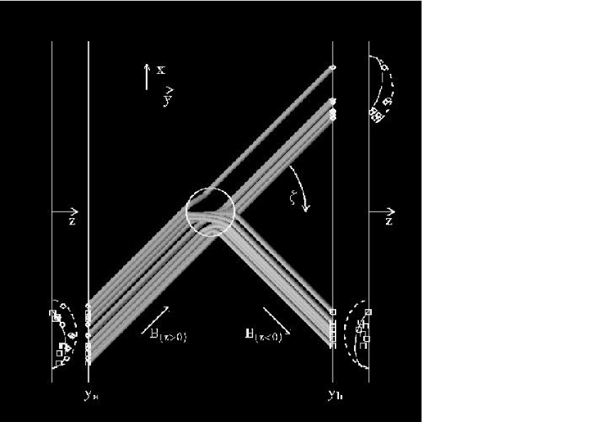
Figure 5: 3D plot of field lines intersecting the sphere of potential reconnected field. The field lines shown all cross the $y_{a}<0$ plane above the current sheet ($z>0$). When the field lines pass through the reconnection sphere they deviate from their straight trajectory. Some are unreconnected, and so cross to $y_{b}>0$ plane above the current sheet, but others have reconnected and so cross the $y_{b}>0$ plane below the current sheet. The points at which they intersect the two $y=constant$ planes are shown on the left and right sides as $x-z$ projections, along with the separatrix curve which separates reconnected from unreconnected field lines in those planes (solid lines), and a dashed curve delineating the edge of the flux which intersects the reconnection sphere.

with $r=(x^{2}+y^{2}+z^{2})^{1/2}$, $\tan\phi=y/x$, and $\cos\theta=z/r$. Here $P^{m}_{n}(\cos\theta)$ is the associated Legendre function. Using this in the expression for the full field (Eq. 2) allows field lines to be traced from a plane $y=y_{a}<-\delta$ into and out of the the reconnection region, and on to a plane $y=y_{b}>\delta$, as shown in Figure 5. Field lines which encounter the reconnection sphere compose two semi-cylinders, on opposite sides of $z=0$. Beginning at $y=y_{a}$ on $z>0$ the field lines break into a reconnected tube which crosses over to $z<0$, and a distorted but unreconnected tube which remains within $z>0$. The separatrix consists of field lines which map to $z=0$ at $r=\delta$.

All field lines in the reconnected flux tube must cross $z=0$ within the sphere. In the normalized field, the magnetic flux crossing the half-plane $z=0,x>0$ is

$$-\int\limits_{-\pi/2}^{\pi/2}d\phi\int\limits_{0}^{\delta}dr\,\left.{\partial\chi_{0}\over\partial\theta}\right|_{\theta=\pi/2}~{}=~{}\sum_{n=1}^{\infty}{4n+1\over(n+1)(2n-1)}\delta[P_{2n}(0)]^{2}~{}\simeq~{}\delta~{}~{}.$$ (13)

The reconnected flux within the tube which crosses from $z<0$ to $z>0$ is therefore

$$\Phi_{tube}=B_{0}\delta^{2}\sin\zeta=\frac{\Phi_{0}}{\pi}\sin\zeta~{},$$ (14)

where $\Phi_{0}=B_{0}\pi\delta^{2}$ is the flux incident on the sphere. The second reconnected flux tube, shown in Figure 5, contains the same flux, so $2\sin(\zeta)/\pi$ of the flux incident on the sphere has reconnected. In the limit $\zeta=\pi/2$, this reduces to the two dimensional limit.

The magnetic energy dissipated by the resistivity is

$$\frac{\Delta E_{d}}{E_{0}}=1-\frac{\pi}{4}\sum_{n=1}^{\infty}\frac{(2n+1)(4n+1)}{(n+1)^{2}(2n-1)^{2}}[P_{l}(0)]^{2}\simeq 0.602~{},$$ (15)

where $E_{0}=\sin^{2}(\zeta)B_{0}^{2}\delta^{3}/6$ is the reconnection component of the initial magnetic energy in the sphere. This is very close to the fraction of energy released by dissipation in the two-dimensional case.

3 POST-RECONNECTION EVOLUTION

3.1 Thin Flux Tube Equations

Prior to the reconnection episode the magnetic field is in mechanical equilibrium, since the magnetic field on both sides of the current sheet is uniform. Following the MRE there are two post-reconnection flux tubes with sharp bends; these are clearly out of equilibrium. The object of the present work is to model the dynamical evolution of these structures, to ascertain how the localized reconnection affects the global field.

Since the reconnection has created flux tubes, one model for their evolution can be sought in the dynamical equations for isolated, thin flux tubes proposed by Spruit, (1981). Such models have traditionally been applied to cases with large plasma $\beta$ where an isolated flux tube is confined by the pressure of unmagnetized surroundings. The underlying approach of considering the net forces acting on segments of a tube should, however, be equally applicable to the present situation, where the flux tube is surrounded by magnetic field, possibly at very small $\beta$.

We characterize one flux tube by its axis ${\bf r}$, parameterized by its arc-length $\ell$. The tube encloses a total axial magnetic flux, $\Phi_{tube}$, in the form of field with strength $B(\ell)$. The field strength is determined by pressure balance across the tube. In low-$\beta$, pressure balance requires that the magnetic field strength within the flux tube match that in the layers between which it is sandwiched: $B(\ell)=B_{0}$. This is the primary respect in which the current case differs from the more conventional, high-$\beta$ case.

A material point, ${\bf r}(\ell)$, accelerates due to the net forces acting on it. If the only force is the imbalance of magnetic tension, resulting from curvature of the field, the governing equation is

$$\left.{\partial{\bf v}\over\partial t}\right|_{\perp}~{}=~{}{B^{2}\over 4\pi\rho}\,{\partial{\bf\hat{t}}\over\partial\ell}~{}~{},$$ (16)

where ${\bf\hat{t}}\equiv\partial{\bf r}/\partial\ell$ is the tangent vector. Writing this in terms of ${\bf r}$ gives a wave equation:

$$\left.{\partial^{2}{\bf r}\over\partial t^{2}}\right|_{\perp}~{}=~{}v_{A}^{2}{\partial^{2}{\bf r}\over\partial\ell^{2}}~{}~{},$$ (17)

where $v_{A}^{2}\equiv B^{2}/(4\pi\rho)$ is the Alfvén speed.

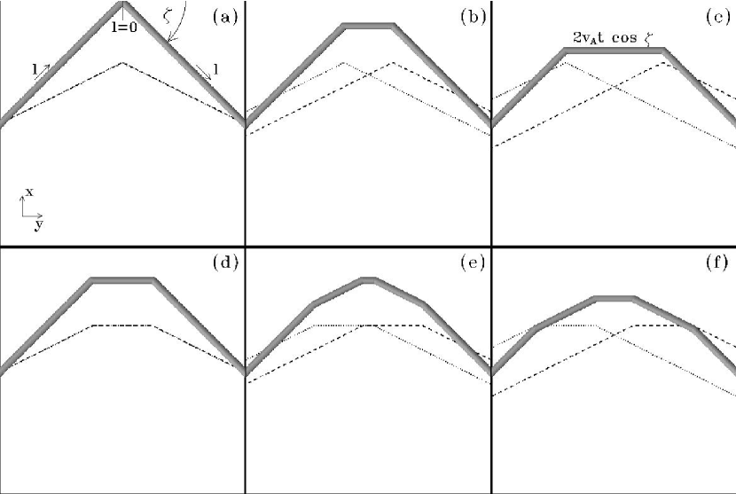
Figure 6: The evolution of two post-reconnection flux tubes according to the thin flux tube dynamics of §3.1. A central segment, between the slow mode shocks formed at the bends in the tube, moves vertically down due to magnetic tension, while the rest of the tube beyond the slow shocks remains fixed. Panels a-c show the motion for a flux tube initially forming the upper part of a triangle, while panels d-f show the motion for a flux tube initially forming the upper part of a trapezoid.

The standard solution to this equation is ${\bf r}={\bf r}(\ell\pm v_{A}t)$. In general, this is the superposition of two waves traveling in opposite directions. As an example, we take the shape shown in Figure 6a,

$${\bf r}(l,0)={\bf r_{0}}-{\bf\hat{x}}|\ell|\sin{\zeta}+{\bf\hat{y}}\ell\cos{\zeta},$$ (18)

as an initial state. The solution to Equation (17) which has this shape and zero velocity at $t=0$ is

$${\bf r}(\ell,t)={\bf r_{0}}-{\bf\hat{x}}\frac{|\ell+v_{A}t|+|\ell-v_{A}t|}{2}\sin{\zeta}+{\bf\hat{y}}\frac{\ell+v_{A}t+\ell-v_{A}t}{2}\cos{\zeta}.$$ (19)

Taking the derivative of Equation (19) with respect to time gives the velocity

$${\bf v}={\bf\hat{x}}{v_{A}\over 2}\sin{\zeta}\left(-\frac{\ell+v_{A}t}{|\ell+v_{A}t|}+\frac{\ell-v_{A}t}{|\ell-v_{A}t|}\right).$$ (20)

Taking the derivative of Equation (19) with respect to $\ell$ gives the tangent vector

$${\bf\hat{t}}=-{\bf\hat{x}}{\rho_{0}\over 2}\left(\frac{\ell+v_{A}t}{|\ell+v_{A}t|}+\frac{\ell-v_{A}t}{|\ell-v_{A}t|}\right)\sin{\zeta}+{\bf\hat{y}}\cos{\zeta}.$$ (21)

Together, these two satisfy Equation (16), generating a set of straight segments, shown in Figure 6a-c. The central segment moves at velocity ${\bf v}=-{\bf\hat{x}}v_{A,0}\sin\zeta$, while the remaining two segments of the tube remain fixed. The corners between segments move at a constant speed $|d\ell/dt|=v_{A,0}$, where $v_{A,0}$ is the Alfvén speed in the stationary segments. In the case where the initial profile forms the hat shape of Figure 6d, as many field lines do in the analytical potential state derived above, the dynamic flux tube consist of five straight segments, as shown in Figure 6e-f.

This analytic solution is a generalization of the two-dimensional solution of Biernat et al., (1987), but differs in several key respects. The slow-mode shocks correspond, in this case, to the bends propagating at the Alfvén speed. These are not simple shocks, owing to the influence of unshocked external field on the tube. It is for that reason that the field strength is unchanged by the bend at low-$\beta$. It is a peculiarity of the two-dimensional case that makes four different shocks, propagating along the four legs of the post-reconnection flux tubes, merge pairwise into two teardrops. Lacking this peculiarity, the three-dimensional case has its full compliment of four separate shocks.

Another important feature of this three-dimensional solution is the absence of snow-plowing. In the two-dimensional model the retracting flux tube sweeps up mass which must be accommodated by an ever-growing bubble (see Fig. 2). In the three-dimensional case, however, the bends move apart to create an expanding region in which to accommodate the new mass. The moving segment between the bends has been shortened by a factor $\cos\zeta$, and so the material on that segment has been compressed to a constant density of $\rho=\rho_{0}/\cos\zeta$, while the tube’s cross section is unchanged (due to the assumed constancy of $B$). A version of the two-dimensional solution might be recovered by setting $\zeta=\pi/2$. However, the divergence in the post-shock density is a signal that the general solution does not include the possibility of an expanding bubble or cross section.

3.2 Energy Release

When the reconnected flux tube retracts, it releases magnetic energy by shortening the length of its field lines. At time $t$ from the reconnection episode, the shock has moved a distance $\lambda(t)=v_{A}t$ along the flux tube in both directions. Or, if the shock has reached the boundary by time $t$, $\lambda$ is simply the original length of the flux tube from the boundary to the reconnection site. The segment of the flux tube exposed to the shocks by this time has an initial length of $2\lambda$, but is shortened by the passage of the shocks to $2\lambda\cos\zeta$ (see Fig. 6). This means that the magnetic energy per reconnected tube has been decreased by $2\Phi_{tube}B_{0}\lambda(1-\cos\zeta)/8\pi$. This energy is converted into the kinetic and thermal energy of the moving flux tube segment, in a manner analogous to the conversion of magnetic energy by the slow-mode shocks in the solution of Biernat et al., (1987). Normalizing energy such that $E^{\prime}\equiv 8\pi E/(B_{0}\Phi_{0})$, the energy released by the retraction of both reconnected tubes is

$$\Delta E_{ft}^{\prime}=\frac{4}{\pi}\lambda\sin(\zeta)(1-\cos\zeta),$$ (22)

where we have set $\Phi_{tube}=\Phi_{0}\sin(\zeta)/\pi$ (Eq. 14). For a small reconnection region, $\delta\ll\lambda$, this is much larger than the energy released in the diffusive reconnection event itself: $\Delta E^{\prime}_{rec}\sim 0.8\delta\sin^{2}(\zeta)$ (Eq. 15).

In addition, the ambient, unreconnected field also releases energy due to the reconnection. When the pair of flux tubes retract from the reconnection region, they vacate a volume of length $2\lambda(1-\cos\zeta)$ and area $2\delta^{2}\sin\zeta$. Unreconnected field then expands slightly to fill the void, meaning that it must weaken slightly. This external field has a pre-expansion energy of

$$E_{ext}=\frac{B_{0}\Phi_{ext}2\lambda(1-\cos\zeta)}{8\pi}.$$ (23)

Here $\Phi_{ext}$ includes all the flux not in the two reconnected tubes, possibly infinite in extent:

$$\Phi_{ext}=B_{0}(A_{full}-2\delta^{2}\sin\zeta),$$ (24)

where $A_{full}$ is the full area of interest, e.g., the simulation area or a significant fraction of the corona. When the reconnected tube retracts, the external field expands to fill the vacated volume, decreasing in strength to $B_{0}-b$ and expanding in area to $A_{full}$ while keeping the same flux. Setting the initial flux (Eq. 24) equal to the final flux ( $[B_{0}-b]A_{full}$), we can solve for the change in field strength:

$$b=\frac{B_{0}A_{full}-B_{0}(A_{full}-2\delta^{2}\sin\zeta)}{A_{full}}=\frac{2B_{0}\delta^{2}\sin\zeta}{A_{full}}.$$ (25)

The energy released by this field is then

$$\Delta E_{ext}=\frac{2b\Phi_{ext}\lambda(1-\cos\zeta)}{8\pi}=\frac{4B_{0}\delta^{2}\sin\zeta}{A_{full}}\frac{B_{0}(A_{full}-2\delta^{2}\sin\zeta)\lambda(1-\cos\zeta)}{8\pi}.$$ (26)

Taking the limit $A_{full}\gg\delta^{2}$, we find that the energy released in the external field is

$$\Delta E_{ext}^{\prime}=\frac{4}{\pi}\lambda\sin(\zeta)(1-\cos\zeta),$$ (27)

which, remarkably, is the same as the energy released in the flux tube itself as it retracts.

3.3 Inclusion of External Forces

The foregoing analysis provides an idealized flux tube evolution following reconnection. To obtain the clean analytic form it assumed that the only force acting on a tube segment is the magnetic tension of the tube itself. There are in general other forces due to the surrounding plasma and un-reconnected field. These forces modify the flux tube dynamics in complicated ways.

To estimate these additional effects, we assume that the solution retains the general form of the idealized one: bends propagate at the Alfvén speed, creating a post-reconnection segment moving with a mean velocity (i.e., center-of-mass velocity) of $V$. The net forces on the post-reconnection segment, or simply “segment”, increase its momentum. If the segment achieves a steady velocity then

$$F_{\rm net}={dP\over dt}\simeq V\frac{dM}{dt},$$ (28)

where $M$ is the total mass of the segment. As the bends move at speed $v_{\rm A}$ along the two tube legs they sweep up mass at a rate

$$\frac{dM}{dt}=2\rho_{0}v_{\rm A}\frac{\Phi_{tube}}{B_{0}},$$ (29)

where $\rho_{0}$ is the density of the ambient plasma, and $\Phi_{tube}/B_{0}$ is the cross sectional area of the tube.

The magnetic tension force along a flux tube, ${\bf F}=\Phi_{tube}{\bf B}/4\pi$, is directed along the axis. The contribution in the direction of motion from a single leg is

$$F_{\rm leg}=\frac{1}{4\pi}\Phi_{tube}B_{\perp},$$ (30)

where $B_{\perp}=B_{0}\sin\zeta$ is the component of the magnetic field along the direction of motion.

There is also a drag force on the segment, which matches the force the segment must exert on the external plasma. It exerts this force in order to deform the un-reconnected flux and to accelerate a wake of entrained fluid. We assume that the work done by these forces is a multiple $X\geq 0$ of the kinetic energy of the segment itself. In terms of this factor the net force can be written

$$F_{\rm net}=\frac{2}{4\pi}\Phi_{tube}B_{\perp}-X{dP\over dt},$$ (31)

and Newton’s law becomes

$$\frac{2}{4\pi}\Phi_{tube}B_{\perp}=2(X+1)V\rho_{0}v_{\rm A}\frac{\Phi_{tube}}{B}.$$ (32)

Solving for the velocity of the segment’s center of mass gives

$$V=\frac{BB_{\perp}}{4\pi\rho v_{\rm A}(X+1)}=\frac{v_{\rm A,\perp}}{X+1}.$$ (33)

Thus even as the bends propagate along this direction at $v_{\rm A,\perp}$, the center of mass of the segment follows behind them at a fraction, $1/(X+1)$, of that speed due to the drag it experiences from its surroundings. This would naturally cause the segment to become arched, but otherwise the behavior would resemble that of the idealized solution.

If the principle external force is one of drag, we can estimate the factor $X$ using the ratio of kinetic energies of the reconnected flux to the un-reconnected flux. Assuming these two components move at similar speed,

$$X=\frac{K_{unrec}}{K_{rec}}.$$ (34)

Inserting this expression for $X$ into Equation (33) then gives us the expected velocity of the tubes. In §5, we calculate this from our simulations to find out how important this added mass effect is.

4 SIMULATIONS

We now use three-dimensional MHD simulations to test the predictions derived above for the dynamics of isolated magnetic reconnection events. We take these simulations in two stages. The first set of simulations reproduce the idealized two-stage process of reconnection and relaxation. These use the reconnected state derived in §2.2 as the initial condition. The initial current sheet therefore has a sphere of potential field on it, as defined by Equation (12), and only a small amount of reconnection take place dynamically, due to the background resistivity of $\delta v_{A}/\eta_{0}=200$. The second set of simulations consider a more realistic case where reconnection and relaxation occur together. These start with an unreconnected current sheet and impose a sphere of high resistivity, $\delta v_{A}/\eta=2$, on the sheet for a short, but finite, time. Once the reconnected flux equals the reconnected flux in the initial state of the potential simulations, this high resistivity region is turned off.

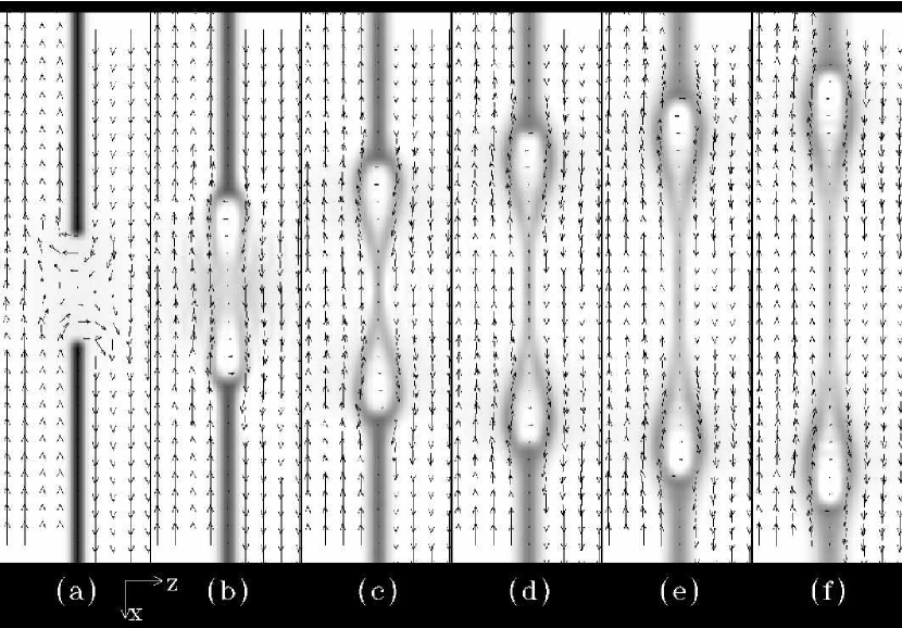
Figure 7: Slices at $y=0$ of magnetic field from the potential reconnection simulation at $\zeta=2\pi/8$, at times $tv_{A\perp}/L=[0.0,0.2,0.4,0.6,0.8,1.0]$. The vectors show the in-plane magnetic field, while the greyscale shows the guide field ($B_{y}$), where black is zero field and white is positive. Panel a shows the initial configuration, including the potential sphere at the center. Panels b-f show the subsequent evolution, as the reconnected fields pull away from this sphere and form into teardrop shapes.

As these simulations have a finite grid size, we cannot simulate the infinitely thin current sheet of Equation (1). Rather, we simulate a finite width Harris current sheet, with a guide field component added. The magnetic field of the current sheet, shown in Figure 7a, is then given by

$${\bf B}=B_{0}\sin(\zeta)\tanh\left(\frac{z}{l}\right){\bf\hat{x}}+B_{0}\cos(\zeta)\tanh\left(\frac{|z|}{l}\right){\bf\hat{y}}.$$ (35)

In this equilibrium, the guide field $B_{y}$ drops to zero at the center of the sheet. We choose this form to represent the scenario where the two legs of a CME collide to form the current sheet, with no flux initially in between them. This configuration naturally generates a current sheet with a thin, zero field region between the two collided flux systems. While we focus primarily on this form of the current sheet, for comparison we also simulate two other guide field profiles. The first is where $B_{y}$ is constant across the current sheet: $B_{y}=B_{0}\cos{\zeta}$. The second is a low-$\beta$ equilibrium, where $|{\bf B}|$ is uniform across the current sheet, requiring that $B_{y}=(B_{0}^{2}-B_{x}^{2})^{1/2}$.

In all simulations, we set the current sheet half-width to be the same as the pixel size: $l/L=1/64$, where the simulation cube is $2L$ on a side, and the simulations are run at $128^{3}$ resolution. The radius of the reconnection sphere is $\delta/L=\pi/16$. The pressure is set such that $p+B^{2}/(8\pi)=constant$. Far from the current sheet, the pressure is $p=p_{0}=20/3$ in units where $B_{0}/(8\pi)^{1/2}=1$ for the high-$\beta$ simulations, and $B_{0}/(8\pi)^{1/2}=4$ for the low-$\beta$ simulations. This gives $\beta=8\pi p_{0}/B_{0}^{2}=20/3$ and $5/12$, respectively. The density is set to be initially uniform everywhere.

We use the MHD code CRUNCH3D (see, e.g., Dahlburg & Norton,, 1995) to carry out these simulations. This code solves the compressible, visco-resistive MHD equations, in the form presented in Linton & Antiochos, (2005), with uniform viscosity, but non-uniform resistivity. The code is pseudo-spectral, and therefore has periodic boundary conditions.

4.1 Potential Reconnected Field

4.1.1 Simulations

For the first set of simulations, the initial state has a sphere of potential, reconnected field imposed on the current sheet, as shown in Figures 7a and 8a. Figure 7 is a $y=0$ cut through the simulation, showing the magnetic field in the plane as the vectors, and the field perpendicular to the plane (the guide field) as the greyscale. Figure 7a shows how the addition of the potential sphere to the current sheet creates a set of reconnected fields, which form an x-point in the midplane of the sphere. These reconnected fields are well out of equilibrium, as there is no force balancing their tension. In Figures 7b and c, these fields therefore quickly pull away from the reconnection region, forming a pair of teardrop shapes. These shapes are fully formed by Figure 7c, meaning that all of the initially reconnected flux has retracted from the reconnection sphere into the teardrop shapes. From then, the reconnected fields simply pull away from the center of the simulation, approximately keeping the same teardrop shape throughout. This dynamic resembles the two-dimensional analytic dynamics of Biernat et al., (1987) (Fig. 2).

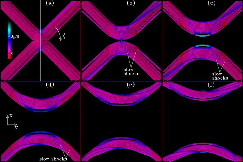
Figure 8: Three dimensional view of the magnetic field lines from the potential reconnection simulation at $\zeta=2\pi/8$, at the same times as in Figure 7. Field lines are traced from Lagrangian particles initially on the $y=0$ plane inside the reconnection sphere. The color is set by the level of current density parallel to the magnetic field, normalized by the maximum initial current density $J_{0}$. The slow mode shocks set up by the reconnection are visible in panels b-d. The white vertical line in panel a shows the location of the $y=0$ cuts of Figure 7.

There is, however, a fundamental difference between the three-dimensional reconnected field shown in Figure 7 and the two-dimensional reconnected field shown in Figure 2. While the envelopes of the teardrop shapes are slow-mode shocks in two dimensions, this is not the case in three dimensions. To see these shocks, one must look at the field lines in a three-dimensional figure, such as Figure 8. Here, a set of Lagrangian trace particles are followed dynamically during the simulation, and field lines are traced from these particles and plotted at the same times as the slices of Figure 7. The trace particles used for this figure initially lie within the reconnected sphere along the $y=z=0$ axis. These field lines are shown from the $-{\bf\hat{z}}$ axis, perpendicular to the view shown in Figure 7. The $y=0$ plane of Figure 7 is represented in Figure 8a by the white line bisecting the reconnected field lines. The color table in this figure is proportional to the field aligned electric current, as shown by the color bar.

Figure 8a shows that, in the initial state, all the field lines from these trace particles are reconnected. Most of the field lines take the shape of the upper part of a trapezoid, with one bend in the field lines as they enter the potential sphere, and a second bend as they exit. The solution for their evolution, given by the thin flux tube equations presented in §3.1, should be the superposition of two oppositely propagating trapezoids, each of half the magnitude of the initial trapezoid, as in Figures 6d-f. The two bends thus propagate in both directions along each field line, giving two pairs of shocks on each flux tube. These are the slow-mode shocks corresponding to that of Petschek, (1964) and Biernat et al., (1987). One of these pairs is indicated in Figure 8b-d by the white lines labeled as ‘slow shocks.’ The field lines do not change their shape significantly before the shock hits them, but then they bend to a new direction as the shock passes them. These shocks quickly propagate out of the two dimensional plane of Figure 7 and therefore do not form the boundary of the teardrop shapes in this two-dimensional cut, in contrast to the two-dimensional shocks of Figure 2.

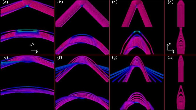
Figure 9: Field lines of the high-$\beta$ reconnection simulations at the four angles simulated: $\zeta=[1,2,3,4]\pi/8$, from left to right. The top halves of panels a-d show the potential simulations in their initial state, while the bottom halves of these panels show the tubes during their evolution at $tv_{A\perp}/L=[0.3,0.6,0.8,0.8]$, respectively. The top halves of panels e-g show the resistive simulations after the same amount of flux has reconnected as was initially reconnected in the potential simulations, at $tv_{A\perp}/L=[0.2,0.3,0.5]$, respectively. Because the flux at $\zeta=4\pi/8$ evolves so quickly once reconnected, the top half of panel (h) is shown at an earlier time, $tv_{A\perp}/L=0.3$, when the reconnected flux equals only half of that reconnected in the potential state. The bottom halves of panels e-h show the reconnected tubes later in their evolution, at $tv_{A\perp}/L=[0.6,0.9,1.1,0.8]$, respectively. Note that panels a-c and e-g show the field lines from the $-{\bf\hat{z}}$ direction while panels d and h, where the guide field is zero, show the field lines from the ${\bf\hat{y}}$ direction.

We performed this simulation, with a potential sphere of reconnection, for angles $\zeta=[1,2,3,4]\pi/8$, as summarized in Figures 9a-d, respectively. Here each panel shows two snapshots from the evolution of a simulation. The top half of each panel shows the initial state of the simulation, and the bottom half of each panel shows the magnetic field in the middle of the evolution. The three simulations with a guide field (a-c) show the slow-mode shock structure discussed above. Panel d, where the guide field is zero, is the closest to the two-dimensional limit, and therefore shows that the field lines form a bulging teardrop shape quite similar to the two-dimensional configuration predicted by Biernat et al., (1987) (Fig. 2).

4.1.2 Analysis

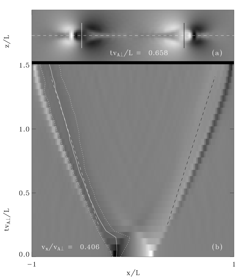
Figure 10: Height versus time stackplot. Panel a shows a $y=0$ slice of $B_{z}$ during the potential reconnection simulation at $\zeta=2\pi/8$. A gaussian is fit to the negative (black) part of $B_{z}$ along the white dashed curve for $x<0$, and this is used to find the center of mass (shown as the white vertical line) of the teardrop shape. Panel b shows cuts along this same dashed line at successive times, stacked on top of each other to give a time-distance plot. The time-distance location of the center of mass is shown as the solid line in this panel, while the $\pm 2\sigma$ level of the gaussian fit is shown as the two dotted lines. The linear least squares fit to the center of mass location, taken from the time the teardrop shape is first fully formed until it first reaches the simulation boundary, is shown as the dashed line. The slope of this line gives the velocity of the reconnected flux tube, $v=0.406v_{A\perp}$.

According to the thin flux tube theory of §3.1, the reconnected flux tubes should retract from the reconnection region at the reconnection Alfvén speed $v_{A\perp}=v_{A}\sin\zeta$. To test this, we measure the speed of the center of the flux tube, i.e., the part lying along the $y=z=0$ axis. Figure 10a shows a slice of $B_{z}$ along the $y=0$ plane, along with a white dashed line along the $y=z=0$ axis. We take the profile of $B_{z}$ along this line at successive timesteps and stack the them vertically to create the distance versus time plot of Figure 10b. In this plot, features moving in the ${\bf\hat{x}}$ direction appear as diagonal lines whose slopes give their ${\bf\hat{x}}$ velocity. To measure the velocity of the center of mass of the flux tube, we fit a gaussian to the x-profile of positive $B_{z}$ along this line on the $x<0$ side of the simulation at each timestep. As an example, the centroid of this gaussian is plotted for $tv_{A\perp}/L=0.658$ in Figure 10a as the vertical white line. This centroid is then plotted as a function of time in Figure 10b as the solid white line, while the $\pm 2\sigma$ level of the gaussian are plotted as the two dotted white lines. We then find the linear least squares fit to this center-of-mass line from the time when the teardrops are first fully formed ($tv_{A\perp}/L=0.27$) until the flux tube is about to hit the edge of the simulation ($tv_{A\perp}/L=1.4$). The fit, plotted for the appropriate time range as the dashed white line in Figure 10b, gives a velocity of $v_{x}=.406v_{A_{\perp}}$.

The asterisks in Figure 11a show the measured velocities of the potential reconnection flux tubes for the four angles simulated. The tube speed is consistently lower than the reconnection Alfvén speed, $v_{A\perp}$, but it approaches this speed as the angle between the reconnecting fields increases. In contrast, the slow-mode shock propagates at the full Alfvén speed, as expected. For $\zeta=\pi/4$, a distance versus time plot with distance along direction of shock propagation, i.e., along the $x=y$ diagonal, gives a shock propagation speed of $.951v_{A}$. As the thin flux tube analysis of §2 predicts that the tube speed should be $v_{A\perp}$ if the shock speed is $v_{A}$, it is clear that there is a drag force, such as the added mass effect, on the tubes. In addition to the tube speed being slower than predicted, a second indication of this drag force is given by the fact that the flux tubes of Figure 8 do not form straight segments between the shocks, but rather form curved segments.

Figure 10 shows an additional feature of the three-dimensional reconnection which may provide an answer to the source of the drag force: the reconnected tubes are sweeping up unreconnected field which lies across their path. This field lies on or close to the current sheet on $z=constant$ planes, in contrast to the reconnected field which crosses the $z=0$ current sheet plane from one set of flux to the other set. The two sets of field are therefore topologically entwined, and wrap around each other rather than flowing over each other. The fact that the reconnected field crosses the $z=0$ plane in one direction forces the unreconnected field it sweeps up to warp such that it crosses $z=0$ in the other direction. This warped field can be seen in Figure 10a. The reconnected field forms the classic teardrop shape, with negative $B_{z}$ on the $x<0$ side and positive $B_{z}$ on the $x>0$ side. But in front of these teardrop shapes the unreconnected, warped fields are visible as a layer of $B_{z}$ of the opposite sign.

The second set of simulations we performed studied the effect of having a stronger guide field in the current sheet. In this case, a magnetic equilibrium was simulated with $\beta=20/3$ as before, but with a uniform guide field, rather than a guide field which drops toward zero in the current sheet. If the tubes are slowed down in part because they drag the guide field in the current sheet along with them, then the flow in this second set of simulations should be slower. Indeed we found that the velocities are slower: $34\%$ for $\zeta=\pi/8$, $16\%$ for $\zeta=2\pi/8$, and $6\%$ for $\zeta=3\pi/8$. Both simulations were exactly the same for $4\pi/8$ because at that angle the guide field is zero everywhere. Thus, we find that the drag effect becomes stronger as the guide field in the current sheet gets stronger.

4.2 Resistively Reconnected Field

The potential reconnection simulations of §4.1 allowed us to study the dynamics of reconnected fields without worrying about the dynamics of the reconnection itself. Having analyzed this simpler situation, we now proceed to study both the reconnection and the subsequent dynamics in the same simulation. Here we start with the same unreconnected state given by Equation (35). But instead of inserting the potential field of Equation (12) into the reconnection sphere, we leave the initial field unreconnected, and increase the resistivity in the sphere ($r\leq\delta$) to

$$\eta=\eta_{0}(1+99e^{-r^{2}/\delta^{2}})$$ (36)

where $\eta_{0}$ is the background resistivity, $\eta_{0}/\delta v_{A}=1/200$. The resistivity stays at this high level until the amount of dynamically reconnected flux equals that which is initially reconnected in the equivalent potential-sphere configuration, and then it is decreased back to $\eta_{0}$.

4.2.1 Two-Dimensional View

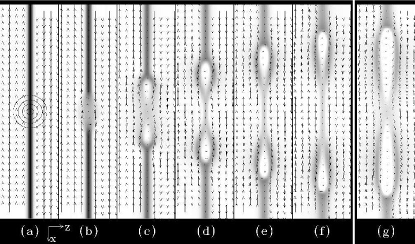
Figure 12: Two dimensional magnetic field slices for the high-$\beta$ resistive simulation at $\zeta=2\pi/8$, in the format of Figure 7. Panels a through g show slices from this simulation at $tv_{A\perp}/L=[0.0,0.05,0.34,0.65,0.96,1.27]$. This shows the evolution of magnetic field which reconnects in a small, 3D sphere in the center of a 1D current sheet. The contours of resistivity are shown in panel a at $10$, $30$, $60$, and $90$ times the background level of $\eta_{0}/(\delta v_{A})=1/200$. The resistive sphere is turned off after panel c, as can be seen by the reformation of the thin current sheet at the center in panel d. The 3D view of this simulation is shown in Figure 15. Panel g shows a cut at $tv_{A\perp}/L=1.29$ from a different simulation with the same initial conditions, but in which the resistive sphere is never turned off.

Two-dimensional snapshots of the magnetic field from such a simulation at $\zeta=2\pi/8$ are shown in Figure 12, in the same format as Figure 7. Panel a shows the unperturbed current sheet, with contours lines of $\eta$ superimposed to show where the resistivity is concentrated. As this sheet will be dissipated by the resistive sphere, it is interesting to follow its structure on the line $x=y=0$, which goes through the center of the resistive sphere. The maximum current strength and the width of the current at half of its maximum value along this line are plotted as a function of time in Figure 13. This shows that the maximum initial value of the current in this sheet is $0.7~{}J_{0}$, where $J_{0}=\nabla\times B=B_{0}\sin\zeta$ is the prescribed initial peak current strength. The initial width of the sheet is $2.7~{}l$ (where $l$ is one pixel wide). Note that the width of the prescribed profile (Eq. 35) is $1.8~{}l$ and so the current sheet is wider and weaker than prescribed by the initial conditions. This is because the code smooths out strongly peaked features with a raised cosine filter as part of the initialization routine.

The effect of the resistive sphere can be seen in Figures 12b and c, where it rapidly diffuses the current sheet, causing it to thicken. Figure 13 shows that the sheet width jumps to between $12~{}l$ and $8~{}l$ while the amplitude drops to $\sim 0.12~{}J_{0}$. The diffusion causes the magnetic field to reconnect, forming a configuration much like that of the potential configuration. This field rapidly pulls away from the reconnection region, as before. This can be seen in Figure 12c where the reconnected flux has started to form into two teardrop shapes on either side of the reconnection region. At this time, the diffusive sphere is still active, and so new flux is being continually added to the reconnected flux tubes, and the teardrop shapes extend back to the x-point.

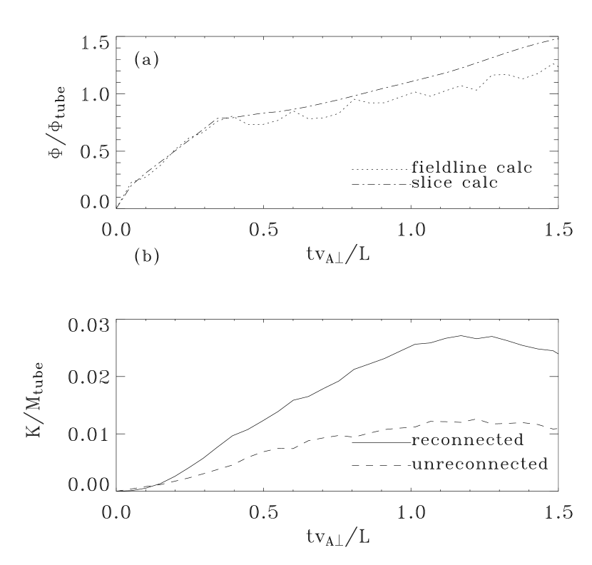
Figure 14: Panel a shows the measured reconnected flux in the high-$\beta$ resistive reconnection simulation at $\zeta=2\pi/8$, normalized by $\Phi_{tube}$ from Equation 14. The dash-dotted line shows the flux calculated from summing over negative $B_{z}$ on the $z=0$ plane at $x<0$. The dotted line shows the flux calculated from the field line summing routine of §5. Panel b shows the global kinetic energies of reconnected (solid) versus unreconnected (dashed) field lines, taken from the fieldline summing routine. These are normalized by the magnetic energy of the two unreconnected flux tubes initially intersecting the reconnection sphere.

The flux reconnected by this diffusion can be estimated by calculating the integral of $B_{z}$ crossing the $z=0$ half plane $x>0$ in the positive direction. This is shown in Figure 14a as the dash-dotted line. At $tv_{A\perp}/L=.34$ as much flux has reconnected ($0.8~{}\Phi_{tube}$) as is reconnected in the initial condition of the equivalent potential reconnection simulation. This is smaller than the value, $\Phi_{tube}$, given by the analytical analysis because the simulated current sheet has finite width $l$, and so the initial flux $\Phi_{0}$ incident on the reconnection sphere is only $80\%$ of that expected for an infinitely thin current sheet. At this time, we turn the resistive sphere off. Reconnection slows significantly at this point, but does not stop, due to the low level of background resistivity.

After the resistive sphere is turned off, the teardrops of reconnected flux continue to move away from the reconnection site, and the current sheet reforms behind them. Interestingly, Figure 13 shows that the width and amplitude of the current sheet return to approximately their initial values.

For comparison with this finite duration magnetic reconnection episode, we simulated the same interaction but never turned off the resistive sphere. The result, at the same time as in Figure 12f is shown in Figure 12g. In this case, the x-point still exists at $x=0$, and the teardrop shape extends all the way back to this x-point. This shows that the aspect ratio of the flux tube cross section is strongly influenced by the duration of the reconnection episode which creates it. The leading edge of this flux tube in panel g has traveled slightly further in the same amount of time than the flux tube with a limited amount of reconnection in panel f. This indicates that the accumulation of extra reconnected flux in the flux tube increases its speed slightly, possibly by helping to overcome the drag force. The current sheet characteristics for this steady reconnection simulation are plotted as the dotted lines in Figure 13. This shows that the width of the sheet settles at about $8~{}l$ and the amplitude stays at about $0.12~{}J_{0}$ as the reconnection approaches a steady-state. The reconnection rate stays the constant through the rest of the simulation rather than slowing down as it does when the resistivity is turned off.

The flux tube velocities for these high-$\beta$ resistive simulations at the four angles $\zeta=[1,2,3,4]\pi/8$ are plotted as the triangles in Figure 11a. These flux tubes are slower than the flux tubes retracting from the potential reconnection region at low angles, yet they are slightly faster at the higher angles.

Again, we repeated this set of simulations for a flat guide field and found the same trend as we did for the potential case: the tubes are slowed by the additional guide field, particularly as $\zeta$ decreases and the guide field gets stronger. Here we found that the velocities were $41\%$ slower for $\zeta=\pi/8$, $17\%$ slower for $\zeta=2\pi/8$, and $12\%$ slower for $\zeta=3\pi/8$.

4.2.2 Three-Dimensional View

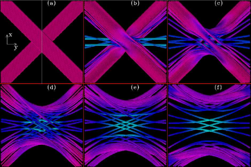
Figure 15: Three dimensional view of field lines from the high-$\beta$ resistive reconnection simulation at $\zeta=\pi/4$, at times $tv_{A\perp}/L=[0.00,0.30,0.60,0.91,1.22,1.53]$. This shows a representative set of field lines which reconnect in the small sphere of high resistivity on the initially 1D current sheet to form two arched loops. The white line in panel a shows the location of the 2D plane of Figure 12.

Figure 15a shows the initial three-dimensional configuration of this simulation, where two sets of straight, unreconnected fieldines cross each other at right angles ($\zeta=\pi/4$). As for Figure 8, these field lines are taken from Lagrangian trace particles, chosen such that they intersect the sphere of high resistivity at the start of the simulation. In this case we show a set which is initially just on either side of the current sheet. As the particles lie in the high resistivity region initially, they are not frozen onto field lines. They do, however, show snapshots of the state of the reconnecting field, and more exactly follow the field line evolution after they leave the resistive sphere, or after the resistive sphere is turned off.

Initially, the fieldines are perfectly straight and unreconnected. As soon as the simulation starts, however, the resistive sphere generates reconnection. The reconnecting field lines ‘fan’ across the current sheet, appearing blue because the current sheet has a very high parallel electric current. This fanning agrees with the analysis and simulations of Pontin et al., (2004) and Pontin et al., (2005). According to this theory, in three dimensions reconnecting field lines continuously change their connectivity while they are actively reconnecting, rather than undergoing a single connectivity-changing event as in two-dimensional reconnection.

The resulting reconnected flux tubes progress in a similar fashion to that of the potentially reconnected field lines. It is difficult to see the slow-mode shocks in this field line figure because the shock fronts are much more diffuse due to the finite time it takes for the reconnection to occur as compared with the instantaneous reconnection in the potential case. However, the shocks can still be followed in diagonal slices of $B_{z}$ along the $x=y$ plane. Again, we find that these shocks travel at close to the full Alfvén speed ($\sim 0.8v_{A}$ for $\zeta=2\pi/8$).

The four simulations of this type are summarized in Figure 9e-h. The top half of each panel shows the reconnected fields early in their evolution, while the bottom half shows the tubes in mid-evolution. The tube dynamics are qualitatively similar to those of the potential sphere simulations shown in Figure 9a-d. A weak shock front can be seen, particularly in the top half of panels e-g, propagating along the flux tubes as in the potential reconnection simulations. In addition, the arched shapes of the reconnected field lines are qualitatively the same in the two types of simulations.

4.3 Low-$\beta$ Simulations

The third set of resistive reconnection simulations we performed are the low-$\beta$ simulations ($\beta=5/12$) where the guide field $increases$ in the current sheet to provide pressure balance there. We were unable to simulate the potential simulation at all angles at the same level of viscosity and resistivity as for the high-$\beta$ simulations, and so we do not discuss this experiment here. The problem is that the fields are very much out of equilibrium at the start of the potential simulation, and there is less gas pressure to balance any sudden disturbances at low-$\beta$ than at high-$\beta$. Therefore the density tends to become negative in cavitation regions of strong motion, causing the code to crash. We could solve this problem through the artificial method of forcing the density to remain larger than some small value. However, as the resistive reconnection simulations do not have the same initial non-equilibrium problem, we focus on those simulations instead.

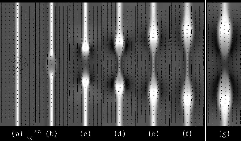
Figure 16: Two dimensional view of the magnetic field in the low-$\beta$ resistive reconnection simulation at $\zeta=\pi/4$, in the format of Figure 7. Panels a through f show this simulation at times $tv_{A\perp}/L=[0.00,0.06,0.34,0.62,0.91,1.20]$. In this case, the current sheet appears white because the guide field is strongest there (to balance the drop in the reconnection component of the field). This contrasts with Figure 7 and 12, where the guide field drops to zero in the current sheet. The field evolves much as it does in the equivalent high-$\beta$ resistive reconnection simulation shown in Figure 12. Again, the resistive sphere is turned off after panel c, and panel g shows a second simulation, in which the resistivity is never turned off, at $tv_{A\perp}/L=1.20$.

The two-dimensional view of the low-$\beta$, resistive reconnection simulation at $\zeta=2\pi/8$ is shown in Figure 16. This shows that decreasing $\beta$ from $20/3$ to $5/12$ does not dramatically affect the reconnection dynamics. The current sheet thickens as before when the resistive sphere is turned on, and two teardrop shaped flux tube cross sections are formed. The current sheet reforms again once the resistive sphere is turned off after Figure 16c. The velocities of these flux tubes are lower than in the high-$\beta$ simulations, as shown by the squares in Figure 11a. In addition, the tube velocities are not significantly faster at high $\zeta$ angles, in contrast to the high-$\beta$ simulations. Finally, for reference, Figure 16g again shows a second simulation wherein the resistive sphere is never turned off, and so the flux tube continues to grow in time. This tube again travels slightly farther during the same time than the tube of Figure 16f, which contains less reconnected flux.

5 ADDED MASS EFFECT

The velocities we derive for all of these simulations pose the question: why are the tubes moving at a slower speed than predicted by the thin flux tube model presented above? A likely possibility is the added mass effect discussed in §3.3. When a body accelerates through an external fluid, as the reconnected flux tubes do here, the external fluid is necessarily also accelerated. This takes extra energy, and therefore slows down the flux tube. If this is correct, we should see that the unreconnected field in the simulation gains kinetic energy in proportion to the kinetic energy of the reconnected field.

To study this, we must separate unreconnected fields from reconnected fields. For each time step at which we want to calculate these kinetic energies, we first trace a volume filling set of field lines, starting from a uniformly distributed grid of $64^{2}$ points at the $y=0$ plane. To ensure that the field lines are volume filling, we trace them in both directions in this plane until they hit the $y=\pm L$ boundaries. As $B_{y}$ is greater than zero at all points in the simulation (for $\zeta\neq\pi/2$), this routine counts each field line only once, as no field line doubles back in the ${\bf\hat{y}}$ direction. To fill the whole simulation volume with field lines, this requires that we trace field lines out of the simulation box in the $x$ direction, making use of the periodic boundary conditions. The $\zeta=\pi/2$ case is more involved to study, as it has no organizing guide field. In this case, we trace all field lines from $z>0$ starting at $x=-L$ (the left hand boundary of the simulation). We trace these field lines until they reach the $x=0$ plane or the $z=0$ plane. Assuming symmetry of $B_{y}$ and $B_{x}$ and anti-symmetry of $B_{z}$ about $x=0$, and symmetry of $B_{y}$ and $B_{z}$ and anti-symmetry of $B_{x}$ about $z=0$ (the simulation shows both are valid) we can recover the whole volume of the simulation without double counting any field lines.

Each field line $i$ from the trace is assigned a flux $d\Phi_{i}$, given by the field strength $B_{i}$ at its starting point $(x_{i},0,z_{i})$ multiplied by an area $4L^{2}/N$, where $N$ is the total number of field lines traced. By integrating local quantities along each field line, we can then find the field line integrated global quantities, such as volume or kinetic energy. The field strength varies along a field line, so we account for the changing area along the field line by assuming a constant flux: $dA_{i}({\bf x})=d\Phi_{i}/|{\bf B}({\bf x})|$. The volume of each field line is then

$$V_{i}=\int dA_{i}dl_{i}=d\Phi_{i}\int\frac{dl_{i}}{|{\bf B}|}.$$ (37)

As a check of our method, we sum over all N field lines to find the total volume. We find that this agrees with the true volume to within $.008\%$ for $N=64^{2}$ field lines. We can then calculate the kinetic energy of each field line:

$$K_{i}=d\Phi_{i}\int\frac{dl_{i}}{|{\bf B}|}\rho|{\bf v}|^{2}.$$ (38)

Summing over the all field lines, we find the kinetic energy agrees with the true sum to within $3.5\%$ on average. We then must divide the field lines into reconnected and unreconnected field lines. Here we take advantage of the simple geometry of our simulation: in the unreconnected state, none of the field lines cross the $z=0$ boundary between the differently directed sets of field lines. Once a field line reconnects, however, it connects fields on both sides of this plane, and so it must intersect this plane. Thus, to categorize field lines as reconnected, we require that they cross the $z=0$ plane in the negative direction for $x<0$ and in the positive direction for $x>0$. This rejects field lines which have wrapped around the reconnected tube but have not reconnected, as they cross the $z=0$ plane in the opposite direction (as discussed in §4.1.2).

The resulting calculations of kinetic energy for the reconnected versus the unreconnected fields are shown in Figure 14 as a function of time for the high-$\beta$ resistive reconnection simulation at $\zeta=2\pi/8$ (see Figs. 12 and 15). Here one can see that the kinetic energy of the reconnected tubes increases in time, and that the kinetic energy of the unreconnected field increases in proportion. Thus, the kinetic energy, and therefore the velocity of the reconnected tubes must be less than it would in the absence of an external medium.

As a check of our field line sorting algorithm, the dotted line in Figure 14a shows the reconnected flux per tube for this simulation, calculated as half the sum of the flux of all reconnected field lines in the field line tracing calculation. This compares reasonably well with the dash-dotted line, which shows the reconnected flux measured by summing all the flux which crosses the $z=0$, $x>0$ plane in the positive direction.

We find that the unreconnected kinetic energy approximately follows the reconnected kinetic energy as in Figure 14b for all simulations studied. To estimate the added mass effect, we calculate the ratio of the integrated kinetic energy for the unreconnected and reconnected field lines:

$$X=\frac{\int K_{unrec}dt}{\int K_{rec}dt}.$$ (39)

where the integrals are taken from the time the flux tubes are fully formed until they are about to reach the boundary. We find that the ratio $X$ increases as $\zeta$ increases. This is further evidence that the guide field is acting as a drag on the flux tubes, as the strength of the guide field decreases as the angle increases.

Using the ratio X in Equations 33 and 34, we calculate the expected velocities of the reconnected tubes due to the added mass effect. The results are shown in Figure 11b. Comparing these velocities with the measured velocities of Figure 11a, we find that, on average, the potential reconnection tubes move at $82\%$ of this predicted speed, the high-$\beta$ resistive reconnection tubes move at $72\%$ of this predicted speed, but the low-$\beta$ resistive reconnection tubes move at only $49\%$ of this speed. Thus we conclude that the added mass effect accounts for most of the flux tube drag at high-$\beta$, but there is an additional, significant source of drag at low-$\beta$.

6 CONCLUSIONS

We have studied non-steady three-dimensional magnetic reconnection by imposing reconnection in a localized sphere on a one-dimensional current sheet. We have shown that external magnetic field intersecting this sphere of reconnection forms a pair of bent, reconnected flux tubes. We have solved analytically for the post-reconnection evolution of these flux tubes, showing that slow-mode shocks propagate as isolated fronts along the legs of the tubes, releasing magnetic energy and accelerating the flux tubes away from the reconnection region. These isolated shock fronts are the three-dimensional generalization of the two V-shaped shocks of steady two dimensional Petschek reconnection (Petschek,, 1964), and of the two teardrop shaped shocks of non-steady two-dimensional reconnection (Biernat et al.,, 1987).

We then studied the evolution of this reconnected magnetic field with three-dimensional magnetohydrodynamical simulations. We found that, as predicted, the reconnected field quickly retracts from the reconnection sphere, accelerating as the slow-mode shock fronts pass by. This accelerated field forms a pair of three-dimensional, arched flux tubes whose cross sections have a distinct teardrop shape. We found that the velocities of these flux tubes are smaller than the reconnection Alfvén speed predicted by the theory, indicating that some drag force is slowing them down. We provide evidence that an added mass effect, wherein the flux tubes sweep up external magnetic field and plasma, is largely responsible for this drag force.

These three-dimensional reconnected flux tubes are a promising candidate for explaining observations of descending coronal voids seen below post-CME flares. Their teardrop shaped cross section is similar to the shape of these voids (McKenzie & Hudson,, 1999), and their three-dimensional arched shape is similar to the shape of the coronal arcade loops formed by these voids later in their evolution (Sheeley et al.,, 2004). We therefore argue that these coronal voids are flux tubes formed by localized patches of reconnection higher in the corona. If this is the case, then by studying the dynamics of these voids, we can directly study the dynamics of reconnected coronal fields. To further explore this possibility, we plan to simulate this patchy reconnection in a two-dimensional Y-type current sheet. In this case, we expect that the reconnected tubes will decelerate as they descend toward the Y-type null and the arcade of field lines below it, much as the coronal voids are observed to do (Sheeley et al.,, 2004). We will compare the deceleration of the simulated tubes with the observed deceleration of the coronal voids, and therefore more accurately test the validity of this model. We will also simulate multiple, simultaneous reconnection events in the same current sheet studying how these tubes interact with each other, and whether their final equilibrium resembles the tangled, sheared equilibrium formed by post-flare coronal loop arcades.

Figure 4: Contours of the normalized flux function $A_{0}(x,z)$, from the real part of Equation 9, showing field lines after a two dimensional reconnection episode. The reconnection region is enclosed by a thick sold line, inside which the field is current-free. Solid lines show the field lines in the two reconnected flux tubes; dashed lines show the unreconnected field lines.

Figure 11: Panel a: measured velocities of the reconnected flux tube velocities. Panel b: predictions of this velocity based on the added mass calculation of §3.3. The asterisks show the velocities from the high $\beta$ potential reconnection simulations with a dip in the guide field at the current sheet. The open triangles show the velocities from the high-$\beta$ resistive reconnection simulations with the same dipped guide field. The open squares show the velocities from the low-$\beta$ resistive reconnection simulations.

Figure 13: Time variation of the current sheet along the $x=y=0$ line through the center of the high-$\beta$ resistive reconnection simulation of Figures 12 and 15. Panel a shows the full width at half of the maximum current value as the solid line. Panel b shows peak current strength in the ${\bf{\hat{y}}}$ direction (solid). The dotted lines in both panels show the width and amplitude of the current sheet if the resistivity in the sphere is never turned off.

References

- Asai et al., (2004) Asai, A., Yokoyama, T., Shimojo, M., & Shibata, K. 2004, ApJ, 605, L77
- Biernat et al., (1987) Biernat, H. K., Heyn, M. F., & Semenov, V. S. 1987, JGR, 92, 3392
- Birn et al., (2001) Birn, J. et al. 2001, JGR, , 3715
- Biskamp, (1986) Biskamp, D. 1986, Phys. Fluids, 29, 1520
- Biskamp & Schwarz, (2001) Biskamp, D. & Schwarz, E. 2001, Phys. Plasmas, 8, 4729
- Carmichael, (1964) Carmichael, H. 1964, in AAS-NASA Symposium on the Physics of Solar Flares, ed. W. N. Hess, (NASA SP-50), 451
- Dahlburg & Norton, (1995) Dahlburg, R. B. & Norton, D. 1995, in Small Scale Structures in Three-Dimensional Hydrodynamic and Magnetohydrodynamic Turbulence, ed. M. Meneguzzi, A. Pouquet, & P. Sulem, (Heidelberg: Springer-Verlag), 331
- Erkaev et al., (2000) Erkaev, N. V., Semenov, V. S., & Jamitsky, F. 2000, Phys. Rev. Let., 84, 1455
- Forbes, (2000) Forbes, T. 2000, JGR, 105, 23153
- Forbes & Acton, (1996) Forbes, T. G. & Acton, L. W. 1996, ApJ, 459, 330
- Gallagher et al., (2002) Gallagher, P. T., Dennis, B. R., Krucker, S., Schwartz, R. A., & Tolbert, A. K. 2002, Sol. Phys., 210, 341
- Heyn & Semenov, (1996) Heyn, M. & Semenov, V. 1996, Phys. Plasmas, 3, 2725
- Hirayama, (1974) Hirayama, T. 1974, Sol. Phys., 34, 323
- Hirose et al., (2001) Hirose, S., Uchida, Y., Uemure, S., Yamaguchi, T., & Cable, S. B. 2001, ApJ, 551, 586
- Hornig, (2005) Hornig, G. 2005, in Reconnection of Magnetic Fields: Magnetohydrodynamics and Collisionless Theory and Observations, ed. J. Birn & E. R. Priest, (Cambridge, UK: Cambridge University Press), pages 24, in press
- Huba, (2005) Huba, J. D. 2005, Phys. Plasmas, 12, 12322
- Innes et al., (2003) Innes, D. E., McKenzie, D. E., & Wang, T. 2003, Sol. Phys., 217, 267
- Klimchuk, (2001) Klimchuk, J. A. 2001, in Space Weather, ed. . H. S. P. Song, G. Siscoe, volume Geophysical Monograph 125, (Washington: AGU), 142
- Kopp & Pneuman, (1976) Kopp, R. A. & Pneuman, G. W. 1976, Sol. Phys., 50, 85
- Kulsrud, (2001) Kulsrud, R. M. 2001, Earth, Planets and Space, 53, 417
- Lin et al., (2003) Lin, J., Soon, W., & Baluinas, S. 2003, JGR, 105, 2375
- Linton & Antiochos, (2005) Linton, M. G. & Antiochos, S. K. 2005, ApJ, 625, 506
- Longcope, (2004) Longcope, D. W. 2004, Quantifying magnetic reconnection and the heat it generates, in Proceedings of the SOHO 15 Workshop – Coronal Heating, ed. R. W. Walsh, J. Ireland, D. Danesy, & B. Fleck, volume 575 of ESA SP, pages 198–209, Paris, European Space Agency
- Low, (2001) Low, B. C. 2001, JGR, 106, 25141
- MacNeice et al., (2004) MacNeice, P., Antiochos, S. K., Phillips, A., Spicer, D. S., DeVore, C. R., & Olson, K. 2004, ApJ, 614, 1028
- McKenzie & Hudson, (1999) McKenzie, D. E. & Hudson, H. S. 1999, ApJ, 519, L93
- Nitta et al., (2002) Nitta, S., Tanuma, S., & Maezawa, K. 2002, ApJ, 580, 538
- Nitta et al., (2001) Nitta, S., Tanuma, S., Shibata, K., & Maezawa, K. 2001, ApJ, 550, 1119
- Parker, (1957) Parker, E. N. 1957, JGR, 62, 509
- Petschek, (1964) Petschek, H. E. 1964, , NASA-SP-50, 425
- Pontin et al., (2005) Pontin, D. I., Galsgaard, K., Hornig, G., & Priest, E. R. 2005, Ph. Plasmas, 12, 052307
- Pontin et al., (2004) Pontin, D. I., Hornig, G., & Priest, E. R. 2004, Geoph. Atroph. Fluid Dynamics, 98, 407
- Scholer & Roth, (1987) Scholer, M. & Roth, D. 1987, JGR, 92, 3223
- Semenov et al., (1983) Semenov, V. S., Heyn, M. F., & Kubyshkin, I. V. 1983, Sov. Astron., 27, 600
- Semenov et al., (1998) Semenov, V. S., Volkonskaya, N. N., & Biernat, H. K. 1998, Phys. Plasmas, 5, 3242
- Sheeley et al., (2004) Sheeley, N. R., Warren, H. P., & Wang, Y.-M. 2004, ApJ, 616, 1224
- Spruit, (1981) Spruit, H. C. 1981, A&A, 98, 155
- Sturrock, (1966) Sturrock, P. A. 1966, Nature, 211, 695
- Sweet, (1958) Sweet, P. A. 1958, Nuovo Cimento Suppl., 8, 188
- Ugai & Tsuda, (1977) Ugai, M. & Tsuda, T. 1977, J. Plasma Phys., 17, 337