Slit Observations and Empirical Calculations for HII Regions

Abstract

When analysing HII regions, a possible source of systematic error on empirically derived quantities, as the gas temperature and the chemical composition, is the limited size of the slit used for the observations. In order to evaluate this kind of systematic error we use the photoionization code Aangaba to create a virtual photoionized region and mimic the effect of a slit observation. A grid of models was built varying the ionizing radiation spectrum emitted by a central stellar cluster, as well as the gas abundance. The calculated line surface brightness was then used to simulate slit observations and to derive empirical parameters using the usual methods described in the literature. Depending on the fraction of the object covered by the slit, the empirically derived physical parameters and chemical composition can be different from those obtained from observations of the whole object. This effect is mainly dependent on the age of the ionizing stellar cluster. The low-ionization lines, which originate in the outer layers of the ionized gas, are more sensitive to the size of the area covered by the slit than the high-ionization forbidden lines or recombination lines, since these lines are mainly produced closer to the inner radius of the nebula. For a slit covering 50% or less of the total area, the measured [O III], [O II] and [O I] line intensities are less than 78%, 62% and 58% of the total intensity for young HII region (t $<$ 3 Myr); for older objects the effect due to the slit is less significant. Regarding the temperature indicator T_[OIII], the slit effects are small ( usually less than 5%) since this temperature is derived from [OIII] high-ionization lines. On the other hand, for the abundance (and temperature) indicator R₂₃, which depends also on the [O II] line, the slit effect is slightly higher. Therefore, the systematic error due to slit observations on the O abundance is low, being usually less than 10%, except for HII regions powered by stellar clusters with a relative low number of ionizing photons between 13.6 and 54.4 eV, which create a smaller O⁺⁺ emitting volume. In this case, the systematic error on the empirical O abundance deduced from slit observations is more than 10% when the covered area is less than 50%.

1 Introduction

For more than 30 years the empirical method for estimating chemical abundances from observed emission line intensities, as proposed by Peimbert & Costero (1969), has been largely used. The method is simple enough to be applied to a wide variety of objects, but can lead to some inconsistencies, as for example the disagreement between abundances derived from forbidden and recombination lines of C and O (Liu et al. 1995, Esteban et al. 2002). However, the method (with some improvements) is very convenient for obtaining a first evaluation of the chemical composition of large samples of objects as planetary nebulae, HII regions and active galactic nuclei. The emitting gas is assumed to have a high- and a low-ionized zones, characterized by the temperature indicated, respectively, by the [O III] and [N II] line intensity ratios. The electron density is usually derived from the [S II] line ratio (see, for instance, Osterbrock 1989). The various ions of the elements present in the gas are assumed to be in either of these regions, following their ionization potential.

As photoionization codes became friendly and available to users (as the well-known Cloudy), several authors prefer to use them for modeling the observed objects, in order to obtain the physical conditions and the chemical composition of the emitting gas. The calculations are usually performed assuming a spherically symmetric object or a plan-parallel slab with a homogeneous density distribution (see for instance Péquignot 1986, Ferland 1995). These models could be considered as an improvement to the empirical method described above.

Spectroscopic observations of HII regions in the Galaxy, as well as in other galaxies, provide a large amount of data on chemical composition (Edmunds & Pagel 1984, van Zee et al. 1998, Kobulnick et al. 1999) as well as on star formation rates (Kennicutt 1992 and Izotov et al. 2004), which are the basis for a better understanding of the chemical evolution of galaxies and of the primordial nucleosynthesis. In the last decade the advent of larger telescopes and modern detectors has increased the precision of the data and raised the expectation for a better understanding of the issues above. On other the hand, the physical parameters derived from observational data of photoionized regions, using empirical methods or one-dimension photoionization models, may introduce systematic errors, decreasing the possibility of reaching the required precision. Some of these systematic errors, which reflect on the elemental abundances, have already been discussed in the literature (Steigman, Viegas & Gruenwald 1997; Viegas, Gruenwald & Steigman 2000; Gruenwald, Steigman & Viegas 2002; Martins & Viegas 2001, 2002). Regarding the star formation rate, a comprehensive analysis of several indicators was recently carried out by Rosa-González, Terlevich & Terlevich (2002).

Most of the emission-line data come from long-slit spectroscopic observations of extended objects. Depending on the distance and on the size of the object, the slit does not cover the whole emitting region and the observed emission-line flux differs from the flux produced by the whole object. Consequently, following the fraction of the area of the nebula covered by the slit (hereafter referred to as slit aperture), the emission line ratios may also differ. Therefore, unless the extended object is far enough to be entirely covered by the slit, the observed emission comes from a slab of gas along the line of sight, with a cross-section equivalent to the slit area projected on the object. In this case, both the empirical method and the photoionization simulations may lead to erroneous results. In fact, the intensity of each line obtained from slit observations come from a different fraction of its emitting volume.

A comprehensive study of the variation of line strengths across an HII region was carried out by Diaz et al. (1987) for NGC 604, the largest H II region in the nearby galaxy M 33. They present line intensities relative to H$\beta$ in five different positions on the nebula. As expected the values vary from point to point, and the derived O/H abundance may differ up to a factor of 2 (see their Table 1, positions A and E).

Another possible source of uncertainty is the effect of atmospheric differential refraction as discussed by Filippenko (1982). In this work, we assume that the slit is in the optimal position.

As part of a program for searching for Wolf-Rayet stars (both WN and WC) in galaxies, long-slit observations were performed for 14 galaxies (Fernandes et al. 2004). The main goal was to study the relation of WR stars and the metallicity, as well as to compare the results with the predictions of evolutionary synthesis models (Schaerer & Vacca 1998). Long-slit observations were performed at the Palomar 200 inch telescope and the 3.6 m ESO/NTT, always using a slit width of 1 arcsec.

Although these observations were aimed to look for the features characterizing the presence of WR stars in the emission-line spectra of star forming regions, the results provide a fair sample of emission-lines that can be used to analyze most of the issues presented above. Since the observed objects are nearby galaxies, any study regarding chemical abundances as well as star formation rates must account for the effect of the area covered by the slit. The observed galaxies are located between 3 and 76 Mpc, except for one galaxy, Mrk 309, at a distance of 170 Mpc. This implies that the fraction of the area covered by the slit is less than 60%, except for the farthest galaxy. Bearing these values in mind, we decided to evaluate the slit effect on the various quantities derived by empirical methods.

Correction of the observational data by a slit aperture effect has been largely discussed in the literature, usually associated to the estimate of the galaxy luminosity (Kochanek, Pahre & Falco 2001; Nakamura et al. 2003; Perez-González et al. 2003; Brinchmann et al. 2004). Here, we analyze the effect of the slit aperture on the empirical methods for chemical abundance determination. A description of how the results from photoionization models can be used to simulate slit observations are presented in §2. The parameters derived from empirical methods are discussed in §3 as a function of the fraction of the area covered by the slit. Concluding remarks appear in §4.

2 Photoionization Models and Slit Simulations

In order to analyze the relationship between the fraction of area covered by the slit and the parameters derived from empirical calculations, we use photoionization models. We assume that the physical conditions and the emission-line intensities obtained by the numerical simulations correspond to the observed data from a virtual nebula. These data are then used to derive parameters by empirical methods, as density and gas temperature, as well as the chemical composition.

The photoionization code Aangaba (Gruenwald & Viegas 1992) is used to simulate HII regions. In order to account for the range of physical parameters found in HII regions, a grid of models is built by varying the shape and intensity of the ionizing radiation spectrum of the central stellar cluster, as well as the gas chemical composition. Spherical symmetry is adopted for calculating the diffuse radiation.

The shape of the ionizing spectrum is related to the age of the young stellar cluster powering the nebula, while the intensity (and the number of ionizing photons per second, Q_H), to its initial mass. Stellar cluster ages of 0.0, 2.5, 3.3, 4.5 and 5.4 Myr (Cid-Fernandes et al. 1992) are used, with Q_H in the range 10⁴⁹ to 10⁵³ photons s^-1. Depending on the stellar cluster age, the corresponding mass spans from 150 to 10⁸ M_⊙. The adopted chemical composition is in the range 0.1 to 1.5 Z_⊙, with solar values from Grevesse & Anders (1989) and Grevesse & Sauval (1998), keeping the solar ratio between the heavy element abundances. The gas density is assumed constant and equal to 100 cm^-3.

The physical conditions are obtained for concentric shells with increasing radii, starting at the inner radius of the nebula and stopping when the gas is neutral (H⁺/H $\leq$ 10^-2). The line-emission intensities are obtained adding the contribution from each shell. The results at the gas outer radius correspond to the total emission-line intensities produced by the virtual nebula. The energy distribution of older clusters (3 $<$ t $<$ 6 Myr) is harder than that of younger clusters, leading to wider recombination zones. Notice, however, that relative number of photons between 13.6 and 54.4 eV for stellar clusters ages t = 2.5 and 5.4 Myr is lower than for other ages. It is then expected that the behaviour of the ionic distribution of O⁺ and O⁺⁺ ions with the slit aperture for t = 5.4 Myr approaches that of t = 2.5 Myr.

The code allows the calculation of line intensities at lines of sight crossing the nebula and characterized by their projected distance from the centre (see Gruenwald & Viegas 1992 for details). These results can then be used to obtain line intensities coming from the region covered by the slit area projected on the nebula, by integrating over the specific studied area. Recall that the virtual nebula is spherically symmetric. Assuming that the slit is centred and its length is longer than the nebula diameter, only the width of the slit limits the volume of gas of each shell contributing to the line intensities. The result for a slit with a projected width larger than the nebula diameter must be equal to the line intensities coming from the whole nebula, thus providing a test for our slit calculations when compared with the results from the nebula simulations.

Once the emission-line intensities are obtained for a slit of a given width, in the following characterized by the fraction of the nebulae covered by the slit, the empirical methods are applied in order to obtain the electron density and temperature of the gas, as well as ionic and elemental abundances.

In order to derive empirical abundances from the observed emission-lines, it is necessary to evaluate the gas temperature. In the method first proposed by Peimbert & Costero (1969), the high-ionization region is characterized by the temperature obtained from the [O III] $\lambda\lambda$4959,5007/$\lambda$4363 emission-line ratio, whereas the low-ionization region by that from the [N II] $\lambda\lambda$6548,6584/$\lambda$5754 emission-line ratio. These line ratios depend on measured auroral line intensities, usually weak and hard to measure mainly in high abundance HII regions where the temperature is low. In this case, another temperature indicator can be used as, for example, R₂₃ = ([O III]$\lambda$5007 + [O II]$\lambda$3737)/H$\beta$ (Pagel et al. 1979) or R₃ = [O III]$\lambda$5007/H$\beta$ (Edmunds & Pagel 1984). Presently, many authors estimate the chemical abundance of oxygen directly from the observed R₂₃ or R₃, using one of the calibrations available in the literature (Edmunds & Pagel 1984, Kobulnick et al. 1999, Pilyugin 2000, 2001 and Kewley & Dopita 2002). Regarding the density, either the [S II] $\lambda$6717/$\lambda$6731 or the [O II] $\lambda$3723/$\lambda$3730 emission-lines ratios are commonly used as indicators. The former is more often used since the two [O II] lines are usually blended.

Since O⁺⁺ and O⁺ are the dominant ions in the HII regions, the oxygen abundance can be obtained once the ionic fractional abundances are derived from the observed lines. Regarding other chemical elements like N and S, not all their ions present in the ionized region are observable. Thus, ionization correction factors (icfs), usually expressed in terms of the abundance of O ions, must be used to access the elemental abundances (Peimbert & Torres-Peimbert 1977 and Peimbert & Torres-Peimbert 1987).

3 Slit Empirical Results

As mentioned above, a grid of HII region models was obtained varying the age and the initial mass of the stellar cluster, as well as the chemical composition of the gas. From the results, the emission-line intensities for a virtual slit projected across the nebula are obtained. The slit size is expressed by the fraction of the total area covered by the slit, and varies from 0 to 1. In order to discuss the effect of slit observations on the results obtained from empirical methods, we first compare the behaviour of measured emission-line intensities of ions at different ionization stages. Line ratios and derived quantities are then analyzed.

3.1 Emission-line intensities

Because the low-ionization lines are produced in the outer zone of the ionized region, their measured intensities are more sensitive to slit aperture effects. Indeed, centred long-slit observations cover a smaller fraction of the emitting volume of the low-ionization lines than that of high-ionization lines, which are produced mainly in the inner zones.

In order to illustrate the effect of the slit aperture on the measured line intensities, their ratios to the total line intensity are shown in Figures 1 and 2 as a function of the fraction of the total area covered by the slit. The recombination lines H$\beta$ and HeII$\lambda$4686 are plotted in Fig. 1, while the forbidden lines [O III]$\lambda$5007+4959, [O II]$\lambda$3727 and [O I]$\lambda$6300+6363 are in Figure 2. The results correspond to models with ionizing stellar clusters of various ages and Q_H = 1.5$\times$ 10⁴⁹ s^-1, adopting gas solar abundance.

The H$\beta$ line is emitted throughout the ionized region and we expect a mild dependence of the measured intensity on the slit aperture. Notice however that the line intensity distribution across the ionized region depends on the shape of the ionizing radiation spectrum, so does the measured intensity for a given slit aperture. As seen in Figure 1a, with a slit covering about 50% of the total area, the measured H$\beta$ intensity is more than 90% of the total H$\beta$ emission for older HII regions, while for younger clusters it is only 75%, since these clusters show a lack of photons with energy higher than 24.6 eV. Regarding the HeII line (Figure 1b), it is only produced by older HII regions in the very inner ionized zone. In fact, even with a slit covering only 30% of the total area, the measured He II line intensity is as high as 90% of the total intensity. In HII regions, the He⁺ distribution across the photoionized gas is very similar to that of H⁺. Thus, the surface brightness distribution of HeI recombination line is similar to that of H$\beta$. For the recombination lines, the results shown in Figure 1 are roughly clustered around two curves depending on the hardness of the ionizing spectrum.

Figure 1: Behaviour of (a) H$\beta\lambda$4861 and (b) He II$\lambda$4686 line intensities with the area of the nebula covered by the slit, A_S, normalized by the value corresponding to the whole nebula, A_T. Both panels show results of models with Q_H = 1.5$\times$ 10⁴⁹ s^-1 and solar abundance; different curves correspond to different stellar ages.

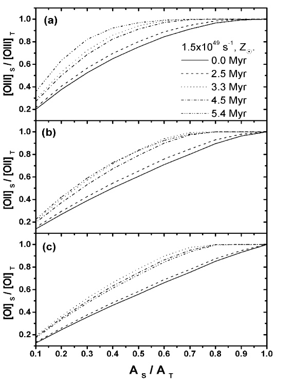
Figure 2: Behaviour of (a) [O III]$\lambda$5007 , (b) [O II]$\lambda$3727 and (c) [O I]$\lambda$6300 line intensities with the area of the nebula covered by the slit. The notation is the same as in Figure 1.

The dependence of the measured [O III], [O II] and [O I] line intensities on the fraction of the area covered by the slit is shown in Figures 2a, 2b and 2c, respectively. The O⁺⁺ ion distribution across the ionized gas is similar to H⁺. However, forbidden lines are strongly dependent on the electron temperature, so the results for [O III] line (Figure 2a) are more dependent on the ionizing spectrum and are not as clustered as in the recombination lines case. Regarding the low-ionization lines (Figures 2b, 2c), which come mainly from the outer parts of the nebula, we expect flatter gradients of the curves compared to those of recombination and high-ionization lines. Indeed, we see that, for a slit covering 50% of the total area, the measured line intensity for [O III], [O II] and [O I] lines are about 78%, 62% and 58% of the total intensity for an young HII region, while it is 95%, 82% and 75% for an older object.

Other low-ionization optical lines like [N II]$\lambda$6584+6548 and [S II]$\lambda$6716+6731, usually used to derive nitrogen and sulphur abundances, show a dependence on the slit aperture similar, respectively, to that of [O II] and [O I] lines.

For Q_H higher than 1.5$\times$ 10⁴⁹ s^-1, the slit effect is more significant. For example, for a covered area of 50%, the H$\beta$ line intensity is about 90% of the total for Q_H = 1.5$\times$ 10⁴⁹ s^-1, while it can reach 70% and 55% for Q_H = 1.5$\times$ 10⁵¹ s^-1 and 1.5$\times$ 10⁵³ s^-1, respectively. The same behaviour is found for the high- and low-ionization forbidden lines. However, for a given slit aperture, the variation of the line intensity with Q_H is smaller for low-ionization lines.

Models with different chemical abundances show that the effect of the slit aperture increases for increasing abundances. Indeed, for a given ionizing spectra, the higher the chemical abundance the farther from the central source is the zone where O⁺⁺ and O⁺ are present and the higher their emission volumes. Thus, in this case, the bulk of their lines comes from the outer regions. It is then expected that higher abundance nebulae are more affected by the slit size.

3.2 Line intensity ratios and empirical temperature

Temperature indicators, like T_[OIII] and R₂₃, as well as empirical abundances are derived from line intensity ratios. Since the line emitting volumes can be different, line ratios can depend on the slit aperture.

The [O III]$\lambda$4363 is characteristic of high temperature zones. Following the ionizing radiation spectrum, its emitting volume may be more concentrated than that of [O III]$\lambda$5007. In this case, we expect that their ratio may vary with the slit aperture. Results for T_[OIII] as a function of the fraction of the area covered by the slit are shown in Figure 3, for models with Q_H = 1.5$\times$ 10⁴⁹, solar abundances, and various stellar cluster ages. It can be noticed that in the case of older clusters (t $>$ 3 Myr), the T_[OIII] fraction is more sensitive to the slit aperture mainly in the case of t = 5.4 Myr. Compared to other old stellar cluster spectra, t = 5.4 Myr has a relatively lower number of photons capable of ionizing H and He, which are more efficient in heating the gas, creating a more concentrated high temperature zone. In this case, only slits covering more than 40% of the total area will result on a temperature value that differs less than 10% from that obtained from observations of the whole nebula. Younger stellar clusters have a negligible number of photons which can produce O⁺⁺, and the emitting volumes of the [O III] lines are similar. In this case, the effect of the slit aperture is negligible. Regarding the temperature indicator R₂₃, since it is mainly dominated by the [O III]/H$\beta$ ratio, its behaviour as a function of the slit aperture is very similar to that of T_[OIII], although, due to the fact that it depends on the low-ionization [O II] line, the systematic uncertainty due to the slit aperture is slightly higher.

For models with Q_H higher than those showed in Figure 3, the slit effect tends to be negligible. Models with gas abundances other than solar show that the slit effect on the intensity ratios is similar or less significant than with solar values.

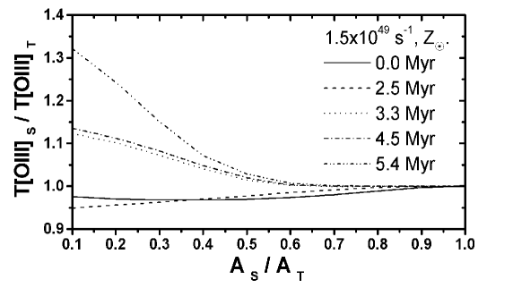
Figure 3: Behaviour of empirical gas temperature, T_[OIII], with the area of the nebula covered by the slit. The notation is the same as in Figure 1.

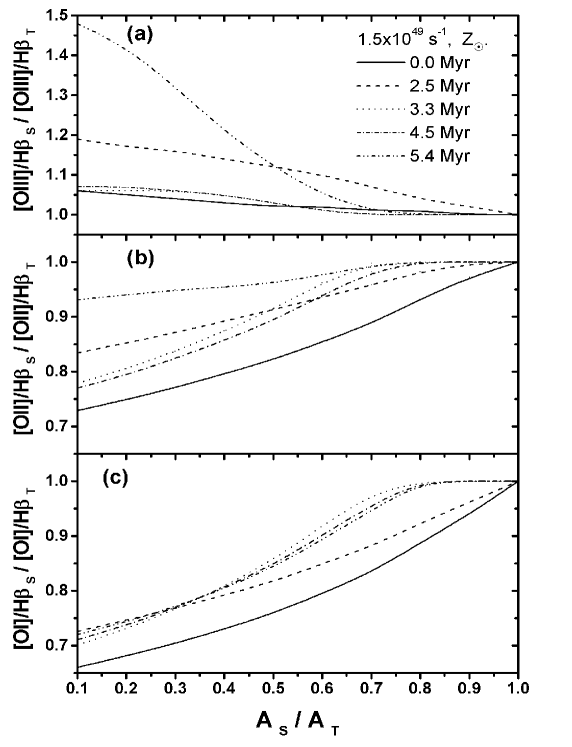
Figure 4: Behaviour of line ratios (a) [O III]$\lambda$5007/H$\beta\lambda$4861 , (b) [O II]$\lambda$3727/H$\beta\lambda$4861 and (c) [O I]$\lambda$6300/H$\beta\lambda$4861 with the area of the nebula covered by the slit. The notation is the same as in Figure 1.

To illustrate the behaviour of low and high ionization lines relative to H$\beta$, the behaviour of O lines is shown in Figures 4a, 4b, and 4c. It can be seen that, as expected, the narrower the slit the more underestimated are the [O I] and [O II] line ratios, since they are produced in the outer zone of the HII region. On the other hand, [O III] is usually overestimated because its emission is more concentrated than that of H$\beta$ emission. The effect is more significant for the two ionizing spectra showing less photons with energy between 24.6 eV and 54.5 eV, i.e., stellar clusters of t = 2.4 and 5.4 Myr.

For a given stellar cluster age, the line ratios obtained from models with higher Q_H or different chemical composition (0.1 to 1.5 Z_⊙) differ less than 10% from those presented in Figures 4.

3.3 Elemental Abundances

It is well known that the oxygen abundance is tightly connected to the gas temperature, since oxygen lines are efficient coolants of the gas. It is then expected that the behaviour of the O/H abundance ratio with the slit aperture is similar to that of T_[OIII], since the [O III] lines are usually produced throughout the nebula. However, the empirical O/H ratio depends also on [O II]/H$\beta$, which is strongly dependent on the area covered by the slit. The volume of the gas emitting [O II], relative to the volume producing [O III], depends on the shape of the ionizing radiation – the larger the amount of high energy photons the larger the recombination zone, thus the larger the O⁺ volume. The empirical O/H is much less dependent on the value of Q_H, which characterizes the intensity of the ionizing radiation, as well as on the adopted chemical composition (Figures 5a, 5b, and 5c).

Because of the similarities of the ionizing spectra for t = 2.5 and 5.4 Myr (see §2), the dependence of the empirical O abundance on the area covered by the slit in these two cases is similar (see Figure 5c). For HII regions ionized by such spectra, the O empirical abundance derived from observations using a slit partially covering the ionized region can be overestimated relative to the abundance derived from observations of the whole nebula. In the case of t = 2.5 Myr the systematic error is about 12% if the fraction of the covered area is less than 50%, while for t = 5.4 Myr this happens for a covered area less than 40% (see Figure 5c). For other cluster ages, the overestimation in the abundance is always less than 5%.

Notice that if the R₂₃ indicator is used, the general behaviour of O/H with the slit aperture is similar to that described above. However, the dependence of R₂₃ on [O II] increases the systematic uncertainty on O/H. Using the O/H - R₂₃ calibration of Kobulnick et al. (1999), the uncertainty is about 12% for 2.5 Myr HII regions if the covered area is less than 40%, very similar to the result obtained with T_[OIII]. However, for the case t = 5.4 Myr, the systematic uncertainty is higher than 10%, as long as the covered area is less than 50%, and linearly increases with decreasing area, reaching 58% when only 10% of the nebula is covered by a centred slit.

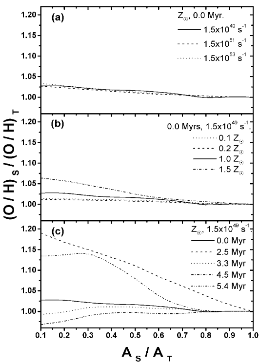
Figure 5: Behaviour of the empirical oxygen abundance, O/H, with the area of the nebula covered by the slit. Each panel shows results of models varying Q_H, the elemental abundances, and the age of the ionizing stellar cluster: (a) young stellar cluster (t = 0 Myr), solar abundance, and three values for Q_H; (b) young stellar cluster (t = 0 Myr), Q_H = 1.5$\times$ 10⁴⁹ s^-1 and elemental abundances from 1.5 to 1/10 solar; (c) Q_H = 1.5$\times$ 10⁴⁹ s^-1, solar abundance and ionizing stellar clusters of various ages from 0 to 5.4 Myr.

The derived He abundance usually varies less than 3% with the slit aperture (Figure 6a). Notice that the He abundance is derived from recombination lines, mostly produced in the ionized gas. Thus, the derived abundance is more sensitive to the shape of the ionizing radiation spectrum than to the gas composition or the ionizing radiation intensity adopted in the models.

Regarding the other elements with observable optical lines, their abundances show a behaviour with the area covered by the slit similar to that presented by O/H (Figures 6b and 6c), as long as the abundance is obtained from low-ionization lines. Such behaviour is expected for N/H and S/H since the measured lines are low-ionization lines and their ionization correction factors are estimated from the O ions. As for O/H, the systematic errors on the empirical abundances derived for N/H and S/H are less than 10%, except for HII regions powered by stellar clusters with a relative low number of photons between 13.6 and 54.4 eV (t = 2.5 and 5.4 Myr).

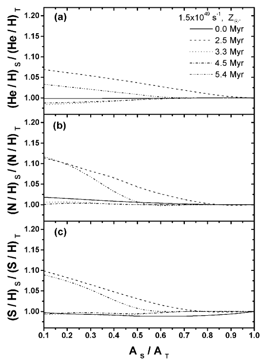
Figure 6: Behaviour of (a) He/H , (b) N/H and (c) S/H empirical abundances with the area of the nebula covered by the slit. The notation is the same as in Figure 1.

4 Concluding Remarks

Because of the development of the instrumentation as well as of the observational techniques, the precision of the observational data available in the last years has increased. Regarding the emission-line regions present in galaxies, empirical methods to derive the physical conditions and the elemental abundances of the emitting gas are largely used. However, although useful, these methods may introduce systematic errors which may be large than the errors expected from the observations.

In this paper we have analyzed one possible source of systematic error, which is the effect the slit size, i.e., the projected area of the slit on the observed object. For this, we used a photoionization code, Aangaba, to create a virtual HII region in order to mimic and to analyze the effect of a slit on the empirically derived properties of the nebula. The procedure adopted in this work is equivalent to that of using a centred long slit, with constant width, to observe the same kind of nebulae located at different distances.

The main results are the following:

(a) The effect of the slit aperture on the empirically derived physical parameters and on the chemical composition is mainly dependent on the age of the ionizing stellar cluster. Because of the characteristics of the spectral energy distribution, the effect is more significant for t = 2.5 and 5.4 Myr.

(b) As expected, the low-ionization lines, which originate in the outer layers of the ionized gas, are more sensitive to the size of the area covered by the slit. Depending on the input parameters of the photoionization model, [O II], [N II] and [S II] emission-lines, relative to H$\beta$, may be underestimated by up to 30% relative to the total emission.

(c) The HeI recombination line intensities, relative to H$\beta$, are less sensitive to the slit width. The difference to the emission of the whole nebula is less than 10%, while for the HeII lines the difference may reach 50 %, since the He⁺⁺ distribution is more concentrated than that of H⁺. For [O III] lines, the effect is highly dependent on the ionizing spectrum.

(d) For the temperature indicators T_[OIII] and R₂₃, the overestimation can be more than 10%, depending on the shape of the ionizing spectrum. In particular for 5.4 Myr HII regions, the systematic error on the O/H is higher when the abundance is derived from R₂₃, reaching 58% for a centred slit covering 10% of the nebula.

(e) The effect of the slit size on the empirical temperatures and on the low-ionization emission-lines reflects on the elemental abundances of O, N and S. For He abundance the effect of the slit aperture is negligible.

In brief, when analyzing a large sample of data on star forming regions using empirical methods, it is necessary to be aware of possible systematic errors introduced by the slit effect. The error is higher the smaller the area covered by the slit, tending to be negligible ($<$ 10%) when the fraction of the covered area is larger than 50%. Remind that for a sample of 14 nearby star-forming galaxies observed with a long slit with a width equal to 1” (Fernandes et al. 2004), the fraction covered by the slit is less than 60%. Other samples of galaxies may also be affected by systematic errors generated by slit observations, and could reflect on the results regarding chemical evolution and star formation rates derived from these samples.

It is also well known that extragalactic HII regions are largely used to derive the primordial He abundance (see for instance, Olive, Steigman & Skillman 1997, Izotov & Thuan 1998) and references therein). These objects are usually distant and the slit used in the observations may cover more than 50% of the area. However, a systematic error on the empirical gas temperature leading to an error on the O/H empirical abundance may lead to a systematic error on the primordial He abundance. This may be significant enough to affect the conclusions drawn from the He primordial abundance derivations (see for instance, Steigman et al. 1997). A deeper analysis of the extragalactic HII region sample is necessary to verify if the slit effect may release the tension between the primordial He and D abundances (Olive, Steigman, Walker 2000).

$Acknowledgements:$ This paper is partially supported by FAPESP (00/06695-0), FAPESP (99/12721-5), CNPq (304077/77-1) and MCT/LNA (381671/2005-4).

References

- [2004] Brinchmann, J.; Charlot, S.; White, S. D. M.; Tremonti, C.; Kauffmann, G.; Heckman, T. & Brinkmann, J. 2004, MNRAS 351, 1151
- [1992] Cid-Fernandes, R., Dottori, H., Gruenwald, R. & Viegas, S. M. 1992, MNRAS 265, 165
- [1984] Diaz, A. I.; Terlevich, E.; Pagel, B. E. J., Vilchez, J. M.; & Edmunds, M. G. 1987, MNRAS, 266, 19
- [1984] Edmunds, M. G. & Pagel, B. E. J. 1984, MNRAS, 211, 507
- [2002] Esteban, C.; Peimbert, M.; Torres-Peimbert, S. & Rodríguez, M. 2002, ApJ 581, 241
- [1995] Ferland, G. 1995, Proc. Of the Space Telescope Science Institute Symposium on The Analysis of Emission Lines: A Meeting in Honor of the 70th Birthdays of D. E. Osterbrock and M. J. Seaton, Eds. R. Williams and M. Livio, Cambridge University Press, p.83
- [2004] Fernandes, I. F.; de Carvalho, R.; Contini, T. & Gal, R. R. 2004, MNRAS 355, 728
- [1984] Filippenko, A. V. 1982, PASP 94, 715
- [1989] Grevesse, N. & Anders, 1989, Proc. of the AIP Conference on Cosmic Abundances of Matter, 183, 1
- [1998] Grevesse, N. & Sauval, A. J. 1998, Sp. Sci. Reviews 85, 161
- [1992] Gruenwald, R. & Viegas, S. M. 1992, APJS 78, 153
- [2002] Gruenwald, R., Steigman, G. & Viegas, S. M. 2002, ApJ 567, 931
- [1998] Izotov, Y. I. & Thuan, T. X. 1998, ApJ 500, 188
- [2004] Izotov, Y. I.; Stasinska, G.; Guseva, N. G.; Thuan, T. X. 2004, A&A 415, 87
- [1992] Kennicutt, R. C. 1992, ApJ 388, 310
- [2002] Kewley, L. J. & Dopita, M. A. 2002, ApJS 142, 35
- [2001] Kochanek, C. S.; Pahre, M. A.; Falco, E. E.; Huchra, J. P.; Mader, J.; Jarrett, T. H.; Chester, T.; Cutri, R. & Schneider, S. E. 2001, ApJ 560, 566
- [1999] Kobulnicky, H. A., Kennicutt Jr., R. C. & Pizagno, J. L. 1999 ApJ 514, 544
- [1995] Liu, X.-W.; Storey, P. J.; Barlow, M. J. & Clegg, R. E. S 1995, MNRAS 272, 369
- [2001] Martins, L. P. & Viegas, S. M. 2001, A&A 361, 1121
- [2002] Martins, L. P. & Viegas, S. M. 2002, A&A 387, 1074
- [2003] Nakamura, O.; Fukugita, M.; Yasuda, N.; Loveday, J.; Brinkmann, J.; Schneider, D. P.; Shimasaku, K. & SubbaRao, M. 2003, AJ 125, 1682
- [1997] Olive, K. A., Steigman, G., & Skillmann, E. D. 1997, ApJ 483, 788
- [2000] Olive, K. A., Steigman, G., & Walker, T. P. 2000, Phys. Reports 333, 389
- [1989] Osterbrock, D. E. 1989, Astrophysics of Gaseous Nebulae and Active Galactic Nuclei (Mill Valley: University Science Books)
- [1979] Pagel, B. E. J.; Edmunds, M. G.; Blackwell, D. E.; Chun, M. S. & Smith, G. 1979, MNRAS 189, 95
- [1969] Peimbert, M. & Costero, R. 1969, Bol. Obs. Tonantzintla y Tacubaya, 5, 3
- [1977] Peimbert, M. & Torres-Peimbert, S. 1977, MNRAS 179, 217.
- [1987] Peimbert, M. & Torres-Peimbert, S. 1987, RMxAA 15, 117.
- [1986] Péquignot, D. 1986, Proc. of the Workshop on Model Nebulae, Ed. D. Péquignot (Paris: Observatoire de Paris), p. 363
- [2003] Pérez-González, P. G.; Gallego, J.; Zamorano, J.; Alonso-Herrero, A.; Gil de Paz, A. & Arag n-Salamanca, A. 2003, ApJ 587, 27
- [2000] Pilyugin, L. S. 2000 A&A 362, 325
- [2001] Pilyugin, L. S. 2001 A&A 374, 412
- [2002] Rosa-González, D., Terlevich, E. & Terlevich, R. 2002, MNRAS 332, 283
- [1998] Schaerer, D. & Vacca, W. D. 1998, ApJ, 497, 618
- [1997] Steigman, G., Viegas, S. M. & Gruenwald, R. 1997, ApJ 490, 187
- [1998] van Zee, L.; Salzer, J. J.; Haynes, M. P.; O’Donoghue, A. A. & Balonek, T. J. 1998, AJ 116, 2805
- [2000] Viegas, S. M., Gruenwald, R. & Steigman, G. 2000, ApJ 531, 813