Abstract

The detection of extraterrestrial neutrinos would confirm predictions that hadronic processes are occurring in high energy astrophysical sources such as active galactic nuclei and gamma-ray bursters. Many models predict a diffuse background flux of neutrinos that is within reach of the AMANDA-II detector. Four years of experimental data (2000 to 2003) have been combined to search for a diffuse flux of neutrinos assumed to follow an E^-2 energy dependence. Event quality cuts and an energy cut were applied to separate the signal hypothesis from the background of cosmic ray muons and atmospheric neutrinos. The preliminary results of this four-year analysis will be presented.

Abstract

Over the past decade, many extragalactic source types have been suggested as potential sources for the ultrahigh energy cosmic ray flux. Assuming hadronic particle acceleration in these sources, a diffuse neutrino flux may be produced along with the charged cosmic ray component. In the presence of a high background of atmospheric neutrinos, no extragalactic neutrino signal has been observed yet. In this paper, a new analysis to investigate with the Antarctic Muon And Neutrino Detector Array (AMANDA-II) a possible extragalactic component in addition to the atmospheric neutrino flux is presented. The analysis is based on the year 2000 data. Using an unfolding method, it is shown that the spectrum follows the atmospheric neutrino flux prediction [1] up to energies above 100 GeV. A limit on the extraterrestrial contribution is obtained from the application of a confidence interval construction to the unfolding problem.

Abstract

The sensitivity of the AMANDA-II detector to ultra high energy (UHE) neutrinos (energy greater than 10⁶ GeV) is derived using data collected during the year 2000. Due to absorption of UHE neutrinos in the earth, the signal is concentrated at the horizon and has to be separated from the background of large muon-bundles induced by cosmic ray air showers. This analysis leads to a sensitivity for an E^-2 all neutrino spectrum (assuming a 1:1:1 flavor ratio) of 3.8 x 10^-7 cm^-2s^-1 sr^-1 GeV for an energy range between 1.8 x 10⁵ GeV and 1.8 x 10⁹ GeV. Sensitivites for five years of data taking and the future IceCube array are given.

Abstract

Besides representing a source of background for the searches of astrophysical objects, atmospheric neutrinos are the most direct calibration source for neutrino telescopes. The characterization of this “test beam” has been, in the past, mostly based on the reconstruction of the energy spectrum and on flux measurements. In this work we investigate the amplitude and phase of possible seasonal variations in the event rate for the sample of 3329 neutrino candidates, detected with the AMANDA-II neutrino telescope in the years 2000-2003 (cfr. the AMANDA-II point source search, this conference). A mechanism that could produce such seasonal variations is the modulation of the target density for interactions of cosmic rays in the atmosphere. Its effect on the atmospheric muon rate is known and measurements have been performed using several underground detectors including AMANDA-II. Its effect on the rate of atmospheric neutrinos at energies above a few hundred GeV has not been studied before. In this paper we report about a calculation of the seasonal variations expected using a global temperature model for the atmosphere. The results are compared to the event rate of the AMANDA-II neutrino sample.

Abstract

In this paper we report the most recent survey of the northern sky to search for neutrino point sources using the AMANDA-II telescope. A search for astrophysical neutrinos of energies above a few tens of GeV was performed on the data collected between the years 2000 and 2003 for a total live-time of 807 days. Thanks to a higher reconstruction accuracy and background rejection power compared to past analyses, together with a longer exposure time, a noticeable improvement has been achieved in the sensitivity of the telescope. The sensitivity to individual point sources, assuming a signal energy spectrum proportional to d$\Phi$/dE $\sim E^{-\gamma}$ with a spectral index of 2, is E${}^{2}\cdot$d$\Phi$/dE$\leqslant 6\cdot 10^{-8}$GeVcm^-2s^-1, weakly dependent on declination. We have obtained a large sample of neutrino candidates with high reconstructed track quality, consisting of 3329 selected up-going events. We searched this sample for a signal from point sources. Individual potential neutrino sources belonging to a catalogue of 33 preselected objects were scanned together with the complete northern sky. We report the outcomes of the individual observations and the significance map of the northern sky.

Abstract

In this paper, we report the first results of an analysis of AMANDA-II data to search for time-variable neutrino point sources. A large sample of 3329 neutrino candidate events from the northern hemisphere was analyzed. The investigation is based on the observation that many cosmic sources have violent variations in their electromagnetic emission. We have tested the hypothesis that neutrino production in such sources is correlated with the electromagnetic activity. Using an independent approach, we have also searched for occasional neutrino flares using a sliding-window technique. Such flares might be detectable with a dedicated time variability investigation and under favorable conditions of signal enhancement and duration. The two search methods will be described and the results reported.

Abstract

Source stacking methods have been applied in $\gamma$-astronomy and in optical astronomy to detect generic point sources at the sensitivity limit of the telescopes. In such an analysis, the cumulative signal and background of several selected sources of the same class is evaluated. In this report we introduce a systematic classification of AGN into several categories that are each considered as a TeV neutrino source candidate. Within each of these AGN categories the individual sources are stacked and tested for a cumulative signal using the AMANDA-II data.

Abstract

Interactions of cosmic rays with the galactic interstellar medium produce high-energy neutrinos through the decay of charged pions and kaons. We report on a search with the AMANDA-II detector for muon neutrinos from the region of the galactic plane below the horizon from the South Pole ($33^{\circ}<$ galactic longitude $<213^{\circ}$). Data from 2000 to 2003 were used for the search, representing a total of 807 days of livetime and 3329 candidate muon neutrino events. No excess of events was observed. For a spectrum of $E^{-2.7}$ and Gaussian spatial distribution ($\sigma=2.1^{\circ}$) around the galactic equator, we calculate a flux limit of $4.8\times 10^{-4}\ \mathrm{GeV}^{-1}\ \mathrm{cm}^{-2}\ \mathrm{s}^{-1}\ \mathrm{sr}^{-1}$ in the energy range from 0.2 to 40 TeV.

Abstract

The Antarctic Muon and Neutrino Detector Array (AMANDA), located at the South Pole, has been searching the heavens for astrophysical neutrino sources (both discrete and diffuse) since 1997. The AMANDA telescope detects Čerenkov radiation caused by high-energy neutrinos traveling through the nearby ice; here we describe AMANDA’s technique to search for neutrinos from gamma-ray bursts, both concurrent with the photon emission and prior to it (during the ”precursor” phase). We present preliminary results from several years (1997-2003) of observations, and we also briefly discuss the current status and future potential of an expanded search for GRBs.

Abstract

The discovery of high-energy (TeV-PeV) neutrinos from gamma-ray bursts (GRBs) would shed light on their intrinsic microphysics by confirming hadronic acceleration in the relativistic jet; possibly revealing an acceleration mechanism for the highest energy cosmic rays. We describe an analysis featuring three models based upon confronting the fireball phenomenology with ground-based and satellite observations of GRB030329, which triggered the High Energy Transient Explorer (HETE-II). Contrary to previous diffuse searches, the expected discrete muon neutrino energy spectra for models 1 and 2, based upon an isotropic and beamed emission geometry, respectively, are directly derived from the fireball description of the prompt $\gamma$-ray photon energy spectrum, whose spectral fit parameters are characterized by the Band function, and the spectroscopically observed redshift, based upon the associated optical transient (OT) afterglow. For comparison, we also consider a model (3) based upon averaged burst parameters and isotropic emission. Strict spatial and temporal constraints (based upon electromagnetic observations), in conjunction with a single, robust selection criterion (optimized for discovery) have been leveraged to realize a nearly background-free search, with nominal signal loss, using archived data from the Antarctic Muon and Neutrino Detector Array (AMANDA-II). Our preliminary results are consistent with a null signal detection, with a peak muon neutrino effective area of $\sim 80$ m² at $\sim 2$ PeV and a flux upper limit of $\sim 0.150\>\text{GeV}/\text{cm${}^{2}/$s}$ for model 1. Predictions for IceCube, AMANDA’s kilometer scale successor, are compared with those found in the literature. Implications for correlative searches are discussed.

Abstract

Using AMANDA-II we have performed a search for $\nu$-induced cascades in coincidence with 73 bursts reported by BATSE in 2000. Background is greatly suppressed by the BATSE temporal constraint. No evidence of neutrinos was found. We set a limit on a WB-like spectrum, $A_{90}^{\rm all\;flavors}$ = 9.5$\times$10^-7 GeV cm^-2 s^-1 sr^-1. The determination of systematic uncertainties is in progress, and the limit will be somewhat weakened once these uncertainties are taken into account. We are also conducting a rolling time-window search for $\nu$-induced cascades consistent with a GRB signal in 2001. The data set is searched for a statistically significant cluster of signal-like events within a 1 s or 100 s time window. The non-triggered search has the potential to discover phenomena, including gamma-ray dark choked bursts, which did not trigger gamma-ray detectors.

Abstract

Data taken with the AMANDA high energy neutrino telescope can be used in a search for an indirect dark matter signal. This paper presents current results from searches for neutralinos accumulated in the Earth and the Sun, using data from 1997-1999 and 2001 respectively. We also discuss future improvements for higher statistics data samples collected during recent years.

Abstract

AMANDA-II data acquisition electronics was upgraded in January 2003 to readout the complete waveform from the buried PMTs using Transient Waveform Recorders (TWR). We perform the same atmospheric neutrino analysis on data collected in 2003 by the TWR and standard AMANDA data acquisition system ($\mu$-DAQ). Good agreement in event rate and angular distribution verify the baseline performance of the TWR system.

Abstract

In the last few years a new Data Acquisition System (DAQ) for the AMANDA-II detector was built and commissioned. The new system uses Flash ADCs and works nearly dead time free (0.015%), compared to 15% dead time for the old DAQ. Up to now, this new DAQ was triggered solely by the existing trigger system. Recently a software trigger was developed to take advantage of the new hardware. The first advantage is the ability to define more complex trigger-settings. A local coincidence trigger will improve the acceptance for low energy neutrinos The second advantage is that the new system can more readily integrate the existing 19 AMANDA strings into the new IceCube observatory.

Abstract

The first new optical sensors of the IceCube neutrino observatory - 60 on one string and 16 in four IceTop stations - were deployed during the austral summer of 2004-05. We present an analysis of the first few months of data collected by this configuration. We demonstrate that hit times are determined across the whole array to a precision of a few nanoseconds. We also look at coincident IceTop and deep-ice events and verify the capability to reconstruct muons with a single string. Muon events are compared to a simulation. The performance of the sensors meets or exceeds the design requirements.

Abstract

The IceCube neutrino observatory will consist of an InIce array of 4800 Digital Optical Modules (DOMs) located in the deep ice at the South Pole, and also an IceTop air shower array of 320 DOMs in 160 ice tanks located on the surface. A 10 inch PMT is housed in each DOM for the detection of Cherenkov light. This paper describes the methods of calibration and characterization of the IceCube PMTs in the laboratory, which are germane to improving the detector resolution and reducing systematic uncertainties. Two dimensional scans on the entire photocathode to map out photon conversion efficiency have been carried out for 60 PMTs. The quantum/collection efficiency has been calibrated in an absolute manner using the Rayleigh scattered light from our newly built chamber filled with nitrogen gas. The charge response of the PMTs at temperatures below freezing has been extensively studied and found to be well represented by the analytical model. All these results have been combined and implemented in the detector Monte Carlo simulation.

Abstract

Astrophysical neutrinos at $\sim$EeV energies promise to be an interesting source for astrophysics and particle physics. Detecting the predicted cosmogenic (“GZK”) neutrinos at 10¹⁶ - 10²⁰ eV would test models of cosmic ray production at these energies and probe particle physics at $\sim$100 TeV center-of-mass energy. While IceCube could detect $\sim$1 GZK event per year, it is necessary to detect 10 or more events per year in order to study temporal, angular, and spectral distributions. The IceCube observatory may be able to achieve such event rates with an extension including optical, radio, and acoustic receivers. We present results from simulating such a hybrid detector.

1 Introduction and Motivation

Currently most of the information on the universe comes from photons, however the detection of cosmic neutrinos would provide a new picture of distant regions of space. Neutrinos travel in straight lines, undeflected by magnetic fields. They interact rarely, making detection challenging. However, if detected, the direction of an extraterrestrial neutrino would point to the particle’s origin. Many theoretical models predict that neutrinos originate in hadronic processes within high energy astrophysical sources such as active galactic nuclei and gamma-ray bursters.

This analysis searches for neutrinos from unresolved sources. This search for a diffuse flux of extraterrestrial neutrinos assumes an E^-2 energy spectrum. Although other models will be assumed in future work, this energy spectrum assumption is based on the theory of particle acceleration in strong shocks [1]. Protons experience first-order Fermi acceleration and interact with protons and photons. The resulting pions are thought to decay into neutrinos that keep the same energy spectrum as the primary [2].

The AMANDA-II detector is a collection of 19 strings buried in the ice at the South Pole [3]. A total of 677 optical modules are attached to these strings between the depths of 1500-2000 m. Each optical module consists of a photomultiplier tube surrounded by a pressure-resistant glass sphere. AMANDA-II has been operating since 2000.

Downgoing muons created when cosmic rays interact in the atmosphere trigger the AMANDA-II detector at the rate of 80 Hz. This saturates any possible extraterrestrial signal that might be seen from the Southern Hemisphere. Hence, upgoing events travelling from the Northern Hemisphere to the detector are selected for this analysis. In this way, the Earth acts as a filter against cosmic ray muons [4]. Sky coverage is restricted to 2$\pi$ sr. However, above the PeV range, the field of view is reduced due to neutrino absorption in the Earth [3].

Muons, created from interacting muon neutrinos, travel long distances in the ice while emitting Cherenkov light. The muon tracks are reconstructed from the detection times with a median space angle resolution of $2^{o}$ [3] when events from the highest cut selection are used. All neutrino flavors can cause hadronic or electromagnetic cascades which appear as a spherical point source of light, however they will not be considered here.

2 Backgrounds

The analysis involved the simulation of several different classes of background events. Monte Carlo simulation of neutrinos in the ice was performed assuming an $E^{-1}$ spectrum. The spectrum was reweighted to model an $E^{-2}$ extraterrestrial neutrino signal with a $\nu_{\mu}$ test flux of $E^{2}dN/dE=1\times$10^-6 GeV cm^-2 s^-1 sr^-1. Atmospheric neutrinos were simulated by reweighting the neutrino events to a steeper $E^{-3.7}$ spectrum. This spectral dependence is common to both atmospheric muons and neutrinos because they are both produced by cosmic ray interactions in the atmosphere.

Sixty-three days of downgoing atmospheric muons were simulated with CORSIKA [5]. Downgoing atmospheric muons can reach AMANDA depth, however they cannot penetrate the Earth from the other hemisphere. In contrast, atmospheric neutrinos from the Northern Hemisphere can reach the detector. Hence, atmospheric muons can be rejected with directional cuts, but atmospheric neutrinos cannot be distinguished from signal in this way. However, because the signal has a harder energy spectrum, both atmospheric muons and neutrinos can be separated from signal by energy-based cuts.

It is also possible that two downgoing muons from independent cosmic ray interactions may occur in the detector within the same detector trigger window. If this occurs, the software will have to guess one incidence direction for the pattern of light produced by two different tracks. The resulting reconstructed direction may be upgoing. These events, known as coincident muons, were simulated for 826 days of livetime.

3 Analysis Optimization and Sensitivity

The 2000 to 2003 search encompassed 807 days of detector livetime. As will be described below, the number of optical modules recording photons was used as an energy-related observable to distinguish extraterrestrial neutrinos from atmospheric backgrounds [6]. Analysis cuts were optimized by studying the signal and background Monte Carlo. In order to satisfy blindness requirements, the Monte Carlo and data were checked for agreement with events triggering less than 80 optical modules (NChannel $<80$), hence leaving the high energy data unbiased.

The analysis began with 7.1$\times 10^{9}$ data events which triggered the detector during this time. Most of these were downgoing muons. All data events underwent an initial track reconstruction in which the software picked a direction of the particle based on the pattern of light the detector recorded. All events with reconstructed zenith angles between $0^{o}$ (travelling straight down) and $80^{o}$ degrees (just above the horizon) were removed.

Figure 1: Above: Number of events as the quality cuts are tightened for 807 days of detector livetime. Cuts become increasingly tighter to the right. The quality cuts were aimed at removing the downgoing atmospheric muons and coincident atmospheric muons from the data. Only events with less than 80 optical modules triggered are shown.

More computer-intensive track reconstructions were performed on the remaining events. Although zenith angle cuts required the events to be upgoing, many downgoing atmospheric muons were misreconstructed as upgoing and remained in the sample. To separate these events from the expected atmospheric and extraterrestrial neutrino signals, events were removed if they did not show the signature of a muon neutrino in the detector. Long muon tracks smoothly emit Cherenkov light. High quality events cause many hits that arrive close to the calculated time for unscattered photons. These hits must be spread evenly along the track and the log likelihood that the track is upgoing rather than downgoing must be high. As the requirements for these parameters were tightened, the number of data events began to look increasingly like the atmospheric and extraterrestrial signal Monte Carlo and less like the downgoing atmospheric muon simulation (see figure 1). The quality cuts were optimized to reject the single and coincident muon backgrounds while preserving the expected signal. Quality cut level 11 was chosen to define the sample used for analysis. After a zenith angle cut at $80^{o}$ degrees, 7,769,850 data events remained in the low-energy (NChannel $<80$) sample, but the event quality cuts reduced this to 2207 data events.

The Feldman-Cousins method for calculating the average upper limit was applied [7]. The Model Rejection Factor is defined as the average upper limit divided by the number of predicted signal events [8] for a $\nu_{\mu}$ signal test flux $E^{2}dN/dE=1\times$10^-6 GeV cm^-2 s^-1 sr^-1. Using the simulation of signal and background, the Model Rejection Factor was calculated as a function of the number of optical modules hit in the detector. The minimum Model Rejection Factor, which indicates the best placement of the NChannel cut to separate signal from background, occurs for NChannel $\geq 100$ (see figure 2). Above this cut, the expected background of 16.2 atmospheric neutrinos leads to an average upper limit of 8.19. Dividing this by the expected signal for the given test flux (86.3 events) leads to a final sensitivity on the $\nu_{\mu}$ flux of $1\times$10${}^{-6}\times 8.19/86.3$ GeV cm^-2 s^-1 sr^-1, or $9.5\times$10^-8 GeV cm^-2 s^-1 sr^-1. The sensitivity (multiplied by three for oscillations) is shown in figure 3 in relation to several other models and analyses. The signal Monte Carlo events that populate the final data set have true neutrino energies between 13 TeV and 3.2 PeV (90% region).

4 Conclusions

With the cuts established and sensitivity determined, the high energy data can be studied. Limits obtained from the analysis of the complete data set will be presented at the conference.

The sensitivity of this four-year analysis is improved by a factor of nine over the limit previously set for one year of experimental data (1997). Limits are closing in on the Waxman-Bahcall bound. In the future, several other models for extraterrestrial neutrino production will also be tested.

Figure 2: Left: Reconstructed zenith angle. The cosine of the zenith angle is shown for all low energy data and Monte Carlo. The number of events for 807 days of livetime is shown on the y-axis before the energy cut. After quality cuts, the data and predicted background show good agreement. At this high quality level, the downgoing atmospheric muons and coincident downgoing muons are nearly entirely removed. Right: Number of channels (optical modules) hit for a signal test flux of $1\times$10^-6 GeV cm^-2 s^-1 sr^-1. This energy related variable is used to separate signal neutrinos from the atmospheric $\nu_{\mu}$ background.

Figure 3: All-flavor neutrino limits and sensitivity on an $E^{2}\frac{dN}{dE}$ plot. Neutrino oscillations are assumed. (1) The MACRO $\nu_{\mu}$ analysis for 5.8 years (limit multiplied by three for oscillations) [9]. (2) The AMANDA-B10 $\nu_{\mu}$ analysis from 1997 (multiplied by three for oscillations) [10]. (3) AMANDA-B10 ultra-high energy neutrinos of all flavors 1997 [11]. (4) AMANDA-II all-flavor cascade limit from 2000 [12]. (5) Baikal cascades 1998 - 2003 [13]. (6) The preliminary results of the 2000 AMANDA-II $\nu_{\mu}$ analysis (multiplied by three for oscillations). The limit is derived after unfolding the atmospheric neutrino spectrum. (7) The sensitivity for AMANDA-II ultra-high energy neutrinos of all flavors 2000. (8) 2000 to 2003 AMANDA-II $\nu_{\mu}$ sensitivity (multiplied by three for oscillations).

[Search for a diffuse flux of non-terrestrial muon neutrinos with the AMANDA detector]Search for a diffuse flux of non-terrestrial muon neutrinos with the AMANDA detector

[K. Münich for the IceCube Collaboration] K. Münich^a for the IceCube collaboration
(a) Institute for Physics, University of Dortmund, D-44221 Dortmund, Germany

Search for a diffuse flux of non-terrestrial muon neutrinos with the AMANDA detector

K. Münich^a for the IceCube Collaboration
(a) Institute for Physics, University of Dortmund, D-44221 Dortmund, Germany Presenter: K. Münich (muenich@physik.uni-dortmund.de),  ger-muenich-K-abs1-og25-oral

1 Introduction

Neutrino-astrophysics has enlarged over the last years the knowledge of neutrinos and their properties. Current experiments are able to measure the neutrino flux from the sun as well as the flux that is produced by cosmic rays interacting with the atmosphere. The aim of high energy neutrino experiments such as AMANDA [2, 3, 4] is to observe an extraterrestrial component of the neutrino spectrum. The AMANDA detector, located at the geographical South Pole, uses the ice as the active volume.
Due to the high atmospheric neutrino flux at energies $E_{\nu}>50$ GeV, a non-atmospheric component has not yet been observed. The atmospheric flux decreases roughly with $E_{\nu}^{-3.7}$ as opposed to the extragalactic contribution, which is expected to be around 1.7 powers flatter, $E_{\nu}^{-2}$. Thus, it is predicted that an additional contribution should become dominant at higher energies. The exact energy at which the extraterrestrial flux exceeds the prediction of the atmospheric one is not known due to the uncertainties in the source properties which would determine the normalization of the neutrino flux.
The diffuse neutrino flux presented is measured with a combination of a neural network and a regularized unfolding [5] as described in [6]. Since the measured neutrino flux corresponds with the expectation of the atmospheric neutrino flux up to an energy of 100 TeV, the question of additional constituents and their exclusion has to be investigated. This paper describes how an upper limit to the neutrino flux from extraterrestrial sources can be obtained. It is shown how the unified approach of Feldman & Cousins can be applied to an unfolding problem to set a 90% confidence belt. Taking into account the statistical behavior of individual events, the probability density functions are calculated using large MC statistics. Finally, a limit on the diffuse muon neutrino and antineutrino flux from extragalactic sources is presented. This limit gives the most restrictive estimate of an upper bound of the neutrino flux among currently existing experiments.

2 Method to obtain a 90% confidence belt

The neutrino energy spectrum is dominated by the background of atmospheric neutrinos. By means of MC studies of atmospheric neutrinos the number of events per energy interval can be estimated. The lower energy threshold of examined events for a potential neutrino signal can be optimized [7]. This leads to a limit on the non-atmospheric neutrino flux using the number of measured events above the optimized threshold. The probability $P$ to measure $n$ events in a certain energy bin for a given mean signal $\mu$ is calculated by using large MC statistics. $P$ is also called probability density function, pdf. Its calculation is described in the following paragraph.

For the year 2000, 21 different signal contributions ranging from $10^{-8}$ GeV cm^-2 s^-1 sr^-1 to
$10^{-6}$ GeV cm^-2 s^-1 sr^-1 are used. The signal contribution $\mu$ is equal to the flux $\phi$ multiplied by $E^{2}$. Each signal contribution $\mu$ is represented by 1000 one-year MC experiments which are altogether equivalent to a data taking of 21000 years. The energy is reconstructed using a combination of neural network and regularized unfolding [6]. The resulting energy distribution is evaluated for each of the 1000 MC experiments per fixed signal contribution, resulting in 21000 energy distributions using all 21 signal contributions. After applying an energy cut the event rate in the remaining bins are summed up and histogramed. The normalized histograms give the searched pdfs. In figure 4 the pdf for two different signal contributions is shown.

(a)                                                                   (b)

Figure 4: Probability density function for two different signal contributions. $(a):2.0\cdot 10^{-7}$ GeV cm^-2 s^-1 sr^-1,
$(b):10^{-6}$ GeV cm^-2 s^-1 sr^-1.

(a)                                                                   (b)

Figure 5: Confidence belt in the signal contribution range of $(a):10^{-8}$GeV cm^-2 s^-1 sr^-1 up to $10^{-6}$GeV cm^-2 s^-1 sr^-1 and $(b):1.26\cdot 10^{-7}$GeV cm^-2 s^-1 sr^-1 up to $3.16\cdot 10^{-7}$GeV cm^-2 s^-1 sr^-1.

For generating a 90% confidence belt the method described in the unified approach by Feldman and Cousins [8] is applied using the probability density functions described above. After reconstruction and unfolding of the energy, confidence belts for different energy cuts are compared and the confidence belt for an energy cut resulting in an energy range of $100$ TeV $<E<300$ TeV shows the best performance. The resulting confidence belt for this cut is illustrated in figure 5(a).

For data taken by AMANDA in the year 2000 optimized point source cuts [9] and a zenith veto at 10 degrees below the horizon have been applied. The resulting sample consists of 570 neutrino events. With the method described above the energy is determined. Inspecting the energy distribution of the data leads to 0.36 events in the energy range of $100$ TeV $<E<300$ TeV. Since the event numbers used for building the confidence belt displayed in figure 5(a) are integer, a limit for 0.36 events can only be derived using further interpolation methods. To avoid this and to get a higher resolution the number of MC events have been enlarged by a factor of 10. This is done in the interesting signal contribution region from $1.26\cdot 10^{-7}$ GeV cm^-2 s^-1 sr^-1 to $3.16\cdot 10^{-7}$ GeV cm^-2 s^-1 sr^-1. With the resulting confidence belt presented in figure 5(b) a definite limit of $2.0\cdot 10^{-7}$ GeV cm^-2 s^-1 sr^-1 can be assigned to a event rate of 0.36.

3 Discussion

From the possible error contribution the systematic uncertainties are dominating. The main contribution to the systematic error is made by the uncertainty of the atmospheric neutrino flux 25%, [10].

Adding the smaller contributions as the uncertainty of the $\nu_{\mu}$ to $\mu$ cross section (ca. $10\%$) to this value and including a maximal contamination by atmospheric neutrinos of the data set ($7\%$), a total systematic error of 30% has to be applied.
This leads to a limit for the AMANDA data of the year 2000 of

$$\phi\cdot E^{2}=2.6\cdot 10^{-7}GeV~{}cm^{-2}~{}s^{-1}~{}sr^{-1}.$$

4 Conclusions

Fig. 6 shows the calculated spectrum and limit in the context of different muon neutrino and anti-neutrino flux predictions. The unfolded neutrino spectrum (circles) is complementary to the Frejus data [11] (squares) which are at lower energies. The black dashed lines in this figure show the horizontal and vertical atmospheric neutrino flux. The upper line represents the horizontal flux, while the prediction for the vertical flux

Figure 6: Reconstructed neutrino spectra and resulting limit for the year 2000 data compared with different flux models

is given with the lower line. The atmospheric flux spectrum above an energy of E $>$ 100 GeV is parameterized according to Volkova [1]. Below this energy the parameterization is given according to Honda et al. [12]. The reconstructed flux contains events from the lower hemisphere except events very near to the horizon and is in good conformity with the atmospheric prediction. In addition to the unfolded flux, an upper limit on the extragalactic neutrino signal of $2.6~{}\cdot~{}10^{-7}$ GeV cm^-2 s^-1 sr^-1 is given. The limit clearly gives restrictions on model 1 (StSa) [13], assuming neutrino production in $p\,\gamma$ interactions in AGN cores. This model with the parameterization as given in [13] can be excluded. Model 2 (MPR-max, [14]) represents the maximum neutrino flux from blazars in photo-hadronic interactions and lies within the sensitivity range of AMANDA. In this context, an upper bound on the flux from these sources were estimated in [14], which is indicated in the figure as the shaded region (Model 3, MPR-bound). The horizontal line represents the limit for sources that are optically thick to $n\gamma$ interactions, $\tau_{n\gamma}>>1$, the lower bound of the shaded region gives the bound for optically thin sources $(\tau_{n\,\gamma}<1)$. In future analyses with a larger data set in AMANDA, it should be possible to set limits lying within the shaded regions, so that the opacity of the sources can be constrained.

[Sensitivity of AMANDA-II to UHE Neutrinos]Sensitivity of AMANDA-II to UHE Neutrinos [L. Gerhardt for the IceCube Collaboration] L. Gerhardt^a for the IceCube Collaboration
(a) Department of Physics and Astronomy, University of California, Irvine, Irvine, CA USA
Presenter: Lisa Gerhardt (gerhardt@cosmic.ps.uci.edu),  usa-gerhardt-L-abs1-og25-oral

Sensitivity of AMANDA-II to UHE Neutrinos

L. Gerhardt^a for the IceCube Collaboration
(a) Department of Physics and Astronomy, University of California, Irvine, Irvine, CA USA Presenter: Lisa Gerhardt (gerhardt@cosmic.ps.uci.edu),  usa-gerhardt-L-abs1-og25-oral

1 Introduction

AMANDA is a large volume neutrino telescope with the capability to search for neutrinos from astrophysical sources [1]. In a previous publication [2] it was shown that neutrino telescopes are able to search for UHE neutrinos (neutrinos with energy greater than 10⁶ GeV). UHE neutrinos are of interest because they are associated with the potential acceleration of hadrons by AGNs [3, 4, 5], are produced by the decays of exotic objects such as topological defects [6] or z-bursts [7] and are guaranteed by-products of the interaction of high energy cosmic rays with the cosmic microwave background [8].

Above 10⁷ GeV the Earth is essentially opaque to neutrinos [9]. This, combined with the limited overburden above AMANDA (approximately 1.5 km), means that UHE neutrinos will be concentrated at the horizon. The background for this analysis consists of bundles of down-going, high energy muons from atmospheric showers. The muons from these bundles can spread over areas as large as 10⁴ m². Separation of signal from the background takes advantage of the fact that signal events have a higher light density than background events, which causes multiple hits in multiple channels. Using this as well as the differences in geometrical acceptance and hit topology it is possible to remove almost all background while retaining a high sensitivity to signal. A previous analysis was performed using the inner ten strings of AMANDA (called AMANDA-B10) [2]. This analysis uses all nineteen strings of AMANDA (called AMANDA-II, for description see [1]). Although the effective area of AMANDA-II is approximately the same as AMANDA-B10 for this analysis, the larger number of optical modules (OMs) offer improved background rejection leading to an improved sensitivity.

2 Experimental and Simulated Data

AMANDA-II collected 6.9 x 10⁸ events between February and November of 2000, with an integrated lifetime of 173.5 days after retriggering and correcting for dead time and periods where the detector was unstable. Of this data 20% was used to develop selection criteria, while the rest, with a lifetime of 138.8 days, is set aside for the final analysis. Two sets of cosmic ray air shower background events were generated using CORSIKA [10]. One set uses composition and spectral indices from [11], i.e. the spectra follows approximately E^-3. In the other set, the statistical error and CPU time were reduced by biasing the Monte Carlo generation in both energy and composition (see [2] for a full description). The UHE neutrinos were generated with energies between 10³ GeV and 10¹² GeV using ANIS [12]. For more details on AMANDA simulation procedures see [1, 2].

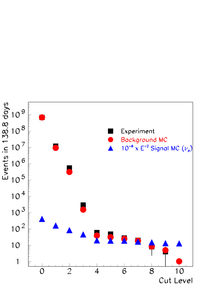
Figure 7: The number of events passing the cuts as a function of cut number. The values for the experimental data are estimated from a 20% subsample. Errors are statistical. The background MC has been scaled by a factor of 1.24 so that the event rate agrees with the experiment at level 0. The signal MC is shown with a lower energy threshold of 10⁵ GeV.

Figure 8: The distribution of primary energy for simulated background at three different cut levels. The data shown is from the biased CORSIKA simulation and demonstrates the removal of lower energy background events by this analysis.

3 Method

Twenty percent of the data from 2000 (randomly selected from February to November) was used to test the agreement with background MC. Following a blind analysis procedure this 20% will be discarded and the developed selection criteria will be applied to the remaining 80% of the data. Final cut values will be chosen by optimizing the model rejection factor [13] for an E^-2 spectrum.

This analysis exploited the differences in light deposition caused by bundles of many low energy muons and single high energy muons. A muon bundle with the same total energy as a single high energy muon spreads its light over a larger volume, leading to a lower light density in the array. Both types of events have a large number of hit channels, but for the same number of hit OMs, the muon bundle has a lower total number of hits (NHITS). It also has a majority of OMs with a single hit, while the signal generates more multiple hits. The number of secondary hits is increased by the tendency of bright signals to produce afterpulses in the photomultiplier tube. The large amount of light deposited by high energy muons is also utilized in the reconstruction. The reconstruction algorithms used by the AMANDA Collaboration are optimized for the reconstruction of low energy muon bundles (from primaries with energies less than approximately 10⁴ GeV), which makes them inaccurate for reconstructing the direction and energy of single high energy muons. However, loose cuts may be placed on the zenith angle based on the expectation that signal will come primarily from the horizontal direction, while background will come from the vertical, down-going direction. Single, high energy muons will also have distinct time residual distributions. The cylindrical geometry of the AMANDA-II array is also used to separate signal from background by estimating arrival direction. Down-going muon bundles will travel along the vertical strings of OMs in AMANDA-II. This, combined with asymmetries in the physical location of strings in the AMANDA-II array, pulls the center of gravity of hits away from the physical center of the array. Light from a single high energy muon will pass through a horizontal cross section of the array striking multiple strings, which pulls the center of gravity of hits closer to the physical center of the array.

Applying cuts on NHITS and the fraction of hit OMs with exactly one hit (F1H) reduced the data samples by a factor of 10³ relative to retrigger level. At this point the data sets are split into a ”high energy” and a ”low energy” sample according to the energy deposited inside the array. A neural net trained on F1H, the closest distance between a reconstructed track and the detector center, and the radial distance from the center of the detector to the center of gravity of hits (RDCOG) served as an estimate of this energy selection value.

The average energy of signal neutrinos in the ”high energy” subset is 10⁸ GeV. The energy deposited inside the array by these neutrinos is much greater than the energy deposited by a typical background event. This allows the application of simple selection criteria to separate signal from background events. Loose cuts on reconstruction variables, F1H and number of hit channels are sufficient to reduce the background expectation to less than 1 event for 138.8 days in this subset.

The ”low energy” subsample consists of neutrinos with an average energy of less than 2 x 10⁶ GeV. As the energy deposited inside the array by a typical background bundle of muons begins to approach the energy deposited by a single astrophysical neutrino, more refined selection criteria which depend on subtleties of the distribution of hit times must be utilized. The production of afterpulses by signal events, combined with the inaccurate reconstruction of signal direction means that UHE neutrino events have an excess of hits with a large time residual relative to the reconstructed track. A cut based on the timing of hits has been devised to take advantage of this. Additionally, for the low energy subsample it is possible to take some advantage of differences in hit topology and multiplicity. Cutting on NHITS, the moment of inertia of the hits and the F1H of a subset of OMs helps to effectively separate signal from background. All these cuts, combined with cuts on reconstruction variables reduced the background by a factor of 10⁸ relative to retrigger level.

As can be seen from figures 8 and  8, this analysis is effective at removing lower energy background events while retaining higher energy signal events.

4 Results and Outlook

Figure 9: Effective area averaged over all angles after all selection criteria have been applied as a function of neutrino energy. The peak in the electron neutrino effective area just below 10⁷ GeV is due to the Glashow resonance.

Figure 10: Limits on the flux of astrophysical neutrinos for an E^-2 spectrum. Shown are the results from the AMANDA B10 diffuse (A) [17] and UHE analyses [2], the AMANDA-II cascade analysis (B) [1], the sensitivity of the three year AMANDA-II diffuse analysis (C) [18], and the expected sensitivities for the AMANDA-II UHE analysis and five years of AMANDA-II. Solid lines indicate the 90% CL limit setting potential for an E^-2 spectrum. Also shown are the expected fluxes from a representative set of models.

Applying all the selection criteria leaves 1.0 + 0.4 background MC event and 0 experimental events in the 20% sample. The expected sensitivity [14] for an E^-2 all neutrino spectrum (assuming a 1:1:1 flavor ratio) is 3.8 x 10^-7 cm^-2 s^-1 sr^-1 GeV with ninety percent of the events between 1.8 x 10⁵ GeV and 1.8 x 10⁹ GeV (fig. 10). This sensitivity is nearly a factor of two improvement over the previous limit set using AMANDA-B10. The expected neutrino effective area (fig. 10) is approximately the same as that of the previous analysis, but this analysis has increased background rejection which leads to an improved sensitivity.

Results from the analysis of the complete year 2000 data will be presented at the meeting. The AMANDA-II detector has been running since the beginning of 2000. Scaling this analysis to five years of AMANDA-II data results in an improvement of the sensitivity by a factor of 4. We expect additional improvements from the TWR system [15] installed at the end of 2002. The TWR system provides additional information which will increase AMANDA-II’s sensitivity to high energy events. For the future, the IceCube detector expects a sensitivity of 4.2 x 10^-9 cm^-2 s^-1 sr^-1 GeV (for 10⁵ GeV to 10⁸ GeV) for three years of operation [16].

An investigation of seasonal variations in the atmospheric neutrino rate with the AMANDA-II neutrino telescope

M.Ackermann^a, E. Bernardini^a for the IceCube Collaboration
(a) DESY Zeuthen, Platanenallee 6, D-15738 Zeuthen, Germany Presenter: Markus Ackermann (markus.ackermann@desy.de), ger-ackermann-M-abs3-he22-poster

[An investigation of seasonal variations in the atmospheric neutrino rate …] An investigation of seasonal variations in the atmospheric neutrino rate with the AMANDA-II neutrino telescope [M. Ackermann and E. Bernardini for the IceCube Collaboration] M.Ackermann^a, E. Bernardini^a for the IceCube Collaboration
(a) DESY Zeuthen, Platanenallee 6, D-15738 Zeuthen, Germany Presenter: Markus Ackermann (markus.ackermann@desy.de), ger-ackermann-M-abs3-he22-poster

1 Introduction

One of the major goals of the large-scale neutrino detectors, AMANDA and IceCube, is to identify cosmic sources of high-energy neutrinos ($>$100GeV). This search is performed by reconstructing the direction of neutrino-induced muons using the pattern of their Cherenkov light emission. Muons and neutrinos produced in the interaction of cosmic rays with the atmosphere form the dominant background for this analysis. Both types of particle are generated in the decay of charged mesons ($\pi^{\pm}$, $K^{\pm}$), which originate in the inelastic scattering of cosmic ray primaries with nuclei of the atmosphere. The muons lose energy by electromagnetic interactions in the ice and rock surrounding the detectors and can therefore not penetrate more than a few kilometers into dense materials. Consequently, this background can be readily removed by restricting the observation to particles travelling in upward direction in the ice. Atmospheric neutrinos however reach the detectors from all directions and can not be distinguished from extra-terrestrial neutrinos. Therefore they remain as a residual background in the data sample, and it is essential to study the properties of this background well to quantify correctly possible deficits and excesses that would be interpreted as neutrino sources.

The search for variations of the atmospheric neutrino rate in time is an example for such a study. We report here on an investigation dedicated to seasonal variations in the atmospheric neutrino rate in the AMANDA-II detector. Annual temperature fluctuations of the atmosphere could be responsible for such variations. We perform a calculation of the expected magnitude of oscillation in the AMANDA-II event rate caused by this effect. The results of these calculations are compared with atmospheric neutrino data from the AMANDA-II neutrino telescope, recorded in 2000-2003 (the data sample used for the point source analysis [1]).

2 Seasonal variations

It has been shown that temperature variations in the atmosphere lead to changes in the intensity of the cosmic ray induced muon flux [3]. This effect has been measured by several experiments, among them MACRO [2] and AMANDA-B10 [4]. Since neutrinos and muons are produced in the same decays one might expect a corresponding variation in the neutrino rate. However, for several reasons the magnitude of these rate oscillations for neutrinos can not be derived directly from the muon rate changes using AMANDA-II or similar detectors:

1. The energy threshold for muons is higher than for neutrinos ($E_{thres}^{\mu}\approx$ 400 GeV, $E_{thres}^{\nu}\approx$ 50 GeV) due to the deep underground location of the detector.

2. For kinematic reasons the atmospheric neutrinos result predominantly from kaon decay, the muons from pion decay [6].

3. The muons originate from the local atmosphere above the detector while neutrinos are observed from interactions anywhere in the earth’s atmosphere.

For these reasons, the analytic high-energy approximations, as used in [2] to calculate the variation in the muon flux, is not valid for neutrinos. At high energy (E $\gg$ 115 GeV for $\pi^{\pm}$, E $\gg$ 850 GeV for $K^{\pm}$) meson interaction dominates over meson decay making the muon and neutrino flux more sensitive to temperature variations [5]. However, for the low energy threshold of AMANDA-II, free decay plays an important role. The meson flux reaches its maximum at an altitude of $X\approx$ 10 - 20 km, so temperature variations at high altitudes have to be taken into consideration. The lack of global high altitude temperature data makes it necessary to use an atmospheric temperature model instead of measurements. There is a variety of such models available ranging from ground to an altitude of several hundred kilometers (an overview can be found at [9]). A numerical calculation is performed here based on the NRLMSISE-00 atmospheric model by [8].

The neutrino flux at a certain atmospheric depth $X$ at energy $E$ produced by $\pi^{\pm}$-decay can be expressed using a derivation given by Gaisser [5]:

$$\Phi_{\nu}(E,X,\theta)=N_{\pi}\;\frac{\epsilon_{\pi}}{(1-r_{\pi})\cos\theta}\int_{E(1-r_{\pi})^{-1}}^{\infty}\;\frac{E^{\prime-2.7}e^{-X/\Lambda_{\pi}}}{XE^{\prime}}\int_{0}^{X}\left(\frac{X^{\prime}}{X}\right)^{\frac{\epsilon_{\pi}}{E^{\prime}\cos\theta}}\exp\left(\frac{X^{\prime}}{\Lambda_{\pi}}-\frac{X^{\prime}}{\Lambda_{n}}\right)dX^{\prime}\;\frac{dE^{\prime}}{E^{\prime}}$$

where $\Lambda_{\pi}$, $\Lambda_{n}$ are pion and nucleon attenuation lengths and $\epsilon_{\pi}$ is the critical energy distinguishing between decay and interaction dominated regimes. $\theta$ is the angle between cosmic ray primary and atmosphere normal, $r_{\pi}=1-m_{\mu}^{2}/m_{\pi}^{2}$ and $N_{\pi}$ is a normalization constant. To compute the neutrino flux produced by kaon decay the constants $\Lambda_{\pi}$, $\epsilon_{\pi}$, $r_{\pi}$ and $N_{\pi}$ have to be replaced by their kaon counterparts. The temperature dependence in this representation is hidden in the critical energy $\epsilon_{\pi}=\epsilon_{\pi}(T(X))$ [2, 5]. The temperature as a function of atmospheric depth $T(X)$ is provided by the NRLMSISE-00 model.

By integrating the equation above, one obtains the total flux above a threshold energy $E_{thres}$. The expected event rate in AMANDA-II is obtained by weighting the energy integral with the effective area of the experiment:

$$n_{\nu}(\theta)=\int_{E_{thres}}^{\infty}A_{eff}(E,\theta)\int_{0}^{\infty}\Phi_{\nu}(E,X,\theta)dEdX$$

The integration of these equations can only be performed numerically; the technique used here is Monte Carlo integration. The neutrino flux is calculated for a grid of $\theta$ ($\theta<60^{\circ}$) and $d$ (day of the year) values. In figure 11 we show some results of this calculation for different threshold energies as well as with an additional weight, accounting for the AMANDA-II effective area. The maximum relative neutrino flux deviation from the mean is shown as a function of geographical latitude in the left plot; the time development for a selected geographical latitude is illustrated on the right. Notice that for neutrinos detected in AMANDA-II there are simple relations between geographical latitude $l$, $\theta$ and the declination $\delta$, which are $\theta=1/2(90^{\circ}-l)$ and $\delta=90^{\circ}-\theta$.

Figure 11: Left plot: Calculated geographical latitude dependence of the amplitude of the seasonal atmospheric neutrino flux variations relative to its annual average. The dotted line corresponds to the flux integrated above 50 GeV, the dashed line to the flux above 1 TeV. The solid line is integrated above 50 GeV but the flux is weighted with a parametrization of the AMANDA-II effective area. Right plot: Calculated time development of the flux variations at a latitude of $65^{\circ}$N (E $>$ 50 GeV, AMANDA-II effective area). The dotted line shows the variation of the $\pi$-decay component alone, the dashed line the K-decay component. The solid line displays the combination of both components.

One can see that the expected variability of neutrino fluxes in AMANDA-II ranges between 3.5% for particles from high latitudes and less than 0.5% from low latitudes, where seasonal temperature changes become very small. The maximum flux for high latitudes is expected around day 190, the minimum flux around day 360. Even for the highest latitudes the variation is considerably smaller than the $\approx 9\%$ seasonal flux variation measured for muons in AMANDA-B10 [4].

3 Comparison to experimental data

The AMANDA-II 2000-2003 point source sample provides a good set of events for investigating seasonal variations in the neutrino rate. While a small fraction of the events in this sample are expected to come from mis-reconstructed muons, the majority forms the largest sample of high energy atmospheric neutrinos available in AMANDA-II. For this analysis the data is divided into 3 angular regions.

declination $\delta$	geogr. latitude $l$	# events	description
$0^{\circ}<\delta\leq 30^{\circ}$	$-90^{\circ}<l\leq-30^{\circ}$	1227	excluded from analysis, bin contaminated
			with misreconstructed down-going muons
$30^{\circ}<\theta\leq 60^{\circ}$	$-30^{\circ}<l\leq+30^{\circ}$	1492	equatorial region
$60^{\circ}<\theta\leq 90^{\circ}$	$+30^{\circ}<l\leq+90^{\circ}$	610	northern hemisphere, high latitudes

The small number of angular bins is due to the limited statistics of 3329 events in the AMANDA-II atmospheric neutrino sample. Figure 12 (right) shows the annual expected relative flux oscillation, from the calculation described above, for the equatorial and high latitudes region. In the high latitude region, $\Delta\Phi_{max}/\Phi$ is approximately 1.2% while for the equatorial region it is below 0.5%. So, in both cases the seasonal variations should be well hidden within the statistical error of the sample. Therefore we can only test if we find data rate variations in AMANDA-II which are incompatible with such a small modulation.

Figure 12: Left plot: Event rates in the AMANDA-II neutrino telescope vs. time coming from geographical latitudes above $30^{\circ}N$ ($\delta>60^{\circ}$) and between $30^{\circ}S$ and $30^{\circ}N$ ($30^{\circ}<\delta\leq 60^{\circ}$). The dotted lines correspond to fits with a constant event rate plus the calculated relative modulation. Right plot: Relative seasonal variations of the atmospheric neutrino flux expected for these latitude bins from the numerical calculations described above.

Figure 12 (left) shows the AMANDA-II event rates in 30 day bins for the two latitude regions (with the years 2000-2003 superimposed in the same bin). These event rates have been corrected for dead-time and down-time of the detector. The distribution is fitted with the calculated intensity variations on top of a constant function. The $\chi^{2}$ for the high latitude bin is $\chi^{2}/n_{free}=6.6/8$, the value for the equatorial bin is $\chi^{2}/n_{free}=8.8/8$. The distributions are compatible with the flux variations calculated.

4 Conclusions

For the first time the expected amplitude of seasonal variations in the atmospheric neutrino rates due to temperature fluctuations was calculated for a high energy neutrino detector. The calculations result in a variation ranging between 0.5% and 3% depending on the geographical latitude, which is too small to be resolved within the limited statistics of high energy atmospheric neutrinos from the AMANDA-II detector. IceCube and other km²-detectors will provide samples with hundreds of thousands of atmospheric neutrinos [7], allowing precision measurements of fluxes. Atmospheric neutrino rate modulations on the 1% level will be measurable with these detectors.

Search for high energy neutrino point sources in the northern hemisphere with the AMANDA-II neutrino telescope

M. Ackermann^a, E. Bernardini^a, T. Hauschildt^b for the IceCube Collaboration
(a) DESY Zeuthen, Platanenallee 6, D-15738 Zeuthen, Germany
(b) Bartol Research Institute University of Delaware, 217 Sharp Lab Newark, DE 19716, USA Presenter: Markus Ackermann (markus.ackermann@desy.de), ger-ackermann-M-abs3-he22-poster

[M. Ackermann et al.] M.Ackermann^a, E. Bernardini^a for the IceCube Collaboration
(a) DESY Zeuthen, Platanenallee 6, D-15738 Zeuthen, Germany Presenter: Markus Ackermann (markus.ackermann@desy.de), ger-ackermann-M-abs2-og25-poster

[Search for high energy neutrino point sources in the northern hemisphere with the AMANDA-II neutrino telescope] Search for high energy neutrino point sources in the northern hemisphere with the AMANDA-II neutrino telescope

[M. Ackermann for the IceCube Collaboration]M. Ackermann^a, E. Bernardini^a, T. Hauschildt^b for the IceCube Collaboration
(a) DESY Zeuthen, Platanenallee 6 D-15738 Zeuthen, Germany
(b) Bartol Research Institute University of Delaware, 217 Sharp Lab Newark, DE 19716, USA Presenter: M. Ackermann (Markus.Ackermann@desy.de), ger-ackermann-M-abs2-og25-poster

1 Introduction

The search for high energy extraterrestrial neutrinos is the major focus of research of the Antarctic Muon And Neutrino Detector Array AMANDA [1]. The goal is the understanding of the origin, propagation and nature of cosmic rays. The elusive nature of neutrinos makes them rather unique astronomical messengers: neutrinos can escape from dense matter regions and propagate freely over cosmological distances. Their observation would also provide an incontrovertible signature of a hadronic component in the flux of accelerated particles. Any source that accelerates charged hadrons to high energy is a likely source of neutrinos: high energy particles will interact with other nuclei or the ambient photon fields producing hadronic showers. In these scenarios, high energy photons and neutrinos are expected to be produced simultaneously. The search for high energy cosmic neutrinos reported in this paper strongly focuses on identified sources of high energy gamma-rays.

Searches for astrophysical sources of neutrinos have to cope with the backgrounds from the interaction of cosmic rays with the Earth’s atmosphere. This results in a background of downward-going muons and a more uniform background of neutrinos from mesons decay. Downward-going muons are rejected by selecting only events that are reconstructed as upward-going, yet an indistinguishable background remains, composed of atmospheric neutrino induced muons and mis-reconstructed downward-going muons. Both sources of background are equivalent within the scope of this work and are treated identically. The final event sample was selected in a blind approach to avoid the enhancement of apparent excesses in the data or the introduction of biases that cannot be statistically described. This was accomplished by randomizing the events in right ascension.

2 Event reconstruction and selection

The major goal of this analysis was the selection of a high statistics sample of high energy events which would be searched for evidence of steady and transient point sources in the northern sky. Event reconstruction and selection were therefore optimized to provide tracks with good angular resolution in a wide energy range. The analyzed data were collected with the AMANDA-II detector between the years 2000 and 2003. Periods corresponding to the detector maintenance activities (roughly from November to February) have not been used. The total live-time, after data quality selection, is 807 days. Details of the pre-processing techniques (hits and Optical Modules selection) and of the reconstruction algorithms can be found in [2].

Neutrino induced up-going tracks were selected by imposing track quality requirements. Event selection criteria were chosen to achieve the best average flux upper limit (“sensitivity” [6]) and were optimized for each declination band independently. Selection criteria included: a parameter describing the hit distribution along the track, the fit likelihood (from two independent track reconstruction procedures) and the event-based angular resolution [5]. The search bin radius in the sky was an additional free parameter. The event selection depends also on energy, due to the energy dependence in the light deposit in the array and a varying detection efficiency. We therefore considered two extreme spectral indexes as reference: $\gamma$=2 and $\gamma$=3. The effects of the different signal spectra on the event cut optimization were investigated separately and the results were combined in the final event selection, to achieve the best performance for both spectra simultaneously. Figure 13 shows the resulting sensitivity and effective area as a function of declination. An overall improvement of about a factor three was obtained compared to the baseline sensitivity of the fully deployed AMANDA-II detector after 197 days of exposure [3].

Figure 13: Left: Sensitivity as a function of declination ($\delta$), for a signal spectral index of 2. The results for individual years and for the combined data sample are shown. Right: Neutrino effective area as a function of the neutrino energy.

A final sample of 3369 events was selected, of which 3329 are up-going. The corresponding directions are shown in Fig. 14 (left). A relatively uniform coverage of the northern sky is obtained.

Figure 14: Left: Sky-plot (in celestial coordinates) of the selected 3329 up-going neutrino candidate events. Right: Significance map from a scan of the northern sky to search for event clusters. The significance is positive for excesses and negative for deficits of events (compared to the expected background).

Due to the event selection optimization allowing wider spectral scenarios compared to [3, 4], this data sample contains a certain contribution from lower energy events.

3 Search for point sources in the northern sky

Candidate	$\delta$(∘)	$\alpha$(h)	$n_{\mathrm{obs}}$	$n_{b}$	$\Phi_{\nu}^{\mathrm{lim}}$	Candidate	$\delta$(∘)	$\alpha$(h)	$n_{\mathrm{obs}}$	$n_{b}$	$\Phi_{\nu}^{\mathrm{lim}}$
TeV Blazars
Markarian 421	38.2	11.07	6	5.6	0.68	1ES 2344+514	51.7	23.78	3	4.9	0.38
Markarian 501	39.8	16.90	5	5.0	0.61	1ES 1959+650	65.1	20.00	5	3.7	1.0
1ES 1426+428	42.7	14.48	4	4.3	0.54
GeV Blazars
QSO 0528+134	13.4	5.52	4	5.0	0.39	QSO 0219+428	42.9	2.38	4	4.3	0.54
QSO 0235+164	16.6	2.62	6	5.0	0.70	QSO 0954+556	55.0	9.87	2	5.2	0.22
QSO 1611+343	34.4	16.24	5	5.2	0.56	QSO 0716+714	71.3	7.36	1	3.3	0.30
QSO 1633+382	38.2	16.59	4	5.6	0.37
Microquasars
SS433	5.0	19.20	2	4.5	0.21	Cygnus X3	41.0	20.54	6	5.0	0.77
GRS 1915+105	10.9	19.25	6	4.8	0.71	XTE J1118+480	48.0	11.30	2	5.4	0.20
GRO J0422+32	32.9	4.36	5	5.1	0.59	CI Cam	56.0	4.33	5	5.1	0.66
Cygnus X1	35.2	19.97	4	5.2	0.40	LS I +61 303	61.2	2.68	3	3.7	0.60
SNR & Pulsars
SGR 1900+14	9.3	19.12	3	4.3	0.35	Crab Nebula	22.0	5.58	10	5.4	1.3
Geminga	17.9	6.57	3	5.2	0.29	Cassiopeia A	58.8	23.39	4	4.6	0.57
Miscellaneous
3EG J0450+1105	11.4	4.82	6	4.7	0.72	J2032+4131	41.5	20.54	6	5.3	0.74
M 87	12.4	12.51	4	4.9	0.39	NGC 1275	41.5	3.33	4	5.3	0.41
UHE CR Doublet	20.4	1.28	3	5.1	0.30	UHE CR Triplet	56.9	11.32	6	4.7	0.95
AO 0535+26	26.3	5.65	5	5.0	0.57	PSR J0205+6449	64.8	2.09	1	3.7	0.24
PSR 1951+32	32.9	19.88	2	5.1	0.21

Table 1: Results from the search for neutrinos from selected objects. $\delta$ is the declination in degrees, $\alpha$ the right ascension in hours, $n_{obs}$ is the number of observed events and $n_{b}$ the expected background. $\Phi_{\nu}^{\mathrm{lim}}$ is the 90% CL upper limits in units of $10^{-8}\mathrm{cm}^{-2}\mathrm{s}^{-1}$ for a spectral index of 2 and integrated above 10 GeV. These results are preliminary (the systematic errors are under assessment).

A search for point sources of neutrinos in the sample of 3329 up-going neutrino candidates was performed by looking for excesses of events from the directions of individual known high-energy gamma emitting objects and by a survey of the full northern sky. In both surveys we used circular search bins, with a size defined by the bin radius optimized together with the event selection for optimal sensitivity. The radius depends on declination and varies between 2.25^∘ and 3.75^∘. The number of events in each declination band is a few hundred and the statistical uncertainty in the background in any given search bin is below 10%.

A sample of 33 candidate neutrino sources have been tested for an excess (or deficit) of events. The investigated sources include galactic and extragalactic objects and their corresponding locations are listed in Tab. 1. The directions of two cosmic rays multiplets (a triplet and the highest energy doublet [7]) were also tested. The background is estimated by averaging in right ascension the event density as a function of declination. A toy Monte Carlo, simulating equivalent tests using sets of events with randomized right ascension values, was used to evaluate the significance of the observations (which expresses the probability of a background fluctuation in units of standard deviations). All the observations are compatible with the expected background. The highest excess corresponds to the direction of the Crab Nebula, with 10 observed events compared to an average of 5.4 expected background (about 1.7 $\sigma$). The probability that a background fluctuation produces this or a larger deviation in any of the 33 search bins is 64%, taking into account the trial factor (due to the multiplicity of the directions examined and the correlation between overlapping search bins).

A full scan of the northern sky was also performed to look for any localized event cluster. We used overlapping search bins with optimal radius and centered on a grid with a spacing of $0.5^{\circ}$. The search was extended up to $85^{\circ}$ in declination. Figure 14 shows a sky map of the 3329 neutrino events and a map of significances from the northern sky cluster search. All the observations are compatible with the background hypothesis. The highest excess corresponds to a significance of about 3.4 $\sigma$. The probability to observe this or a higher excess, taking into account the trial factor, is 92%.

4 Summary and outlook

We performed a search for a signal from point sources of neutrinos in the northern sky with data from the AMANDA-II neutrino telescope. Improved event reconstruction and selection techniques have been applied to the data collected between the years 2000 and 2003. Special emphasis has been put on the energy spectrum of the Monte Carlo events passing the selection cuts, to be sensitive to the largest variety of possible signal energy distributions. The achieved sensitivity to point sources is the most relevant numerical outcome of this analysis, and is equal to E${}^{2}\cdot$d$\Phi$/dE$\leqslant 6\cdot 10^{-8}$GeVcm^-2s^-1, after 807 days of exposure and assuming a signal spectral index of 2. The sensitivity is weakly dependent on declination. We have obtained a large sample of neutrinos with high energies, consisting of 3329 selected up-going events. No statistically significant excess has been observed in the search for a signal from either candidate sources from a catalogue of pre-selected objects or in the full northern sky. We are currently extending this analysis to the data collected in the year 2004. An investigation of the possible sources of systematic uncertainties is also in progress and the upper limits reported here will be updated to account for the systematic error.

Three other contributions to this conference present preliminary results on searches with the four years sample of 3329 events for a variable signal from candidate neutrino sources [8], for a cumulative excess for classes of objects from predefined source catalogues (source stacking analysis) [9] and for a neutrino signal from the galactic plane [10].

Multiwavelength comparison of selected neutrino point source candidates

M. Ackermann^a, E. Bernardini^a, T. Hauschildt^b, E. Resconi^a for the IceCube Collaboration
(a) DESY Zeuthen, Platanenallee 6, D-15738 Zeuthen, Germany
(b) Bartol Research Institute University of Delaware, 217 Sharp Lab Newark, DE 19716, USA Presenter: M. Ackermann (Markus.Ackermann@ifh.de), ger-ackermann-M-abs1-og25-oral

[Multiwavelength comparison of selected neutrino point source candidates]Multiwavelength comparison of selected neutrino point source candidates [M. Ackermann et al.] M. Ackermann^a, E. Bernardini^a, T. Hauschildt^b, E. Resconi^a for the IceCube Collaboration
(a) DESY Zeuthen, Platanenallee 6, D-15738 Zeuthen, Germany.
(b) Bartol Research Institute University of Delaware, 217 Sharp Lab Newark, DE 19716, USA.

Presenter: M. Ackermann (Markus.Ackermann@ifh.de), ger-ackermann-M-abs1-og25-oral

1 Introduction

TeV neutrino candidate sources often show large and violent variations in the electromagnetic emission. Under the assumption that neutrino emission shows a similar variability, a set of methods that test the flare behavior of a source have been developed. Under favorable conditions of signal enhancement and period duration, such flares might be detectable with a dedicated time-variability investigation and still not be evident in the time-integrated point-source search [1].
The driving criteria used for the selection of the sources considered in this analysis are: the source presents an evident variable character in one or more wavelengths, flares are plausible in the period of interest for this analysis (2000-2003) and the total time of the flare periods is long enough in order to allow a reasonable detection probability. Three categories of sources have been selected: blazars, microquasars and variable sources from the EGRET catalog.
Two different methods have been developed in order to search for a variable neutrino signal from these families of sources: (A) a multiwavelength comparison when the source presents a resolved variability in one or more wavelengths, (B) a search for neutrino flare with a sliding-time window when the variable character of the source is evident but electromagnetic observations are limited.
The test data sample is provided by the time-integrated point source search [1]. In the multiwavelength method (A) an appropriate re-optimization for shorter live-times is performed. The complete catalog of sources used in this approach with the results obtained are reported in Table 1. The analysis has been performed following the principle of ”blind analysis” to avoid the introduction of biases that cannot be statistically quantified. Details about this topic are discussed in [1].

2 Method A: Multiwavelength Comparison

A multiwavelength comparison has been developed in order to analyze TeV blazars and microquasars in the scenario of non-steady-state neutrino emission. Details of the method that are specific to these families of sources are reported below.

TeV blazars show dramatic variability correlated between multiple wavelengths of the electromagnetic spectrum; correlations between TeV $\gamma$-rays and X-rays occur on time-scales of hours or less. This correlated variability is often interpreted as a strong argument in favor of pure electromagnetic models (leptonic models) in which the same population of ultra-relativistic electrons is responsible for production of both X-rays and TeV $\gamma$-rays. In fact, these observations do not rule out models involving the acceleration and interaction of protons (hadronic models see e.g. [3]). In hadronic models, pions produced by $p\gamma$ or $pp$ interaction result in the simultaneous emission of $\gamma$-rays and neutrinos. Imaging atmospheric Cherenkov telescopes have detected various $\gamma$-ray flares in the energy region GeV to TeV. If it were not for large gaps in time between the measurements of these flaring periods, the measured on-times of the $\gamma$-rays would clearly define the high state of activity of the sources. On the contrary, the use of the $\gamma$-ray measurements in this context is quite limited. TeV and X-ray flares are, with few exceptions, well correlated (see e.g. [6]), and all-sky X-ray measurements guarantee a quasi-continuous data record. Therefore a reasonable strategy, which we used, is to select the periods of interest on the basis of the X-ray light curves provided by ASM/RXTE [4], see Fig. 15 We have looked for an excess of events in the on-source direction by comparing the integrated number of neutrino counts versus the estimated atmospheric neutrino background for the selected time periods. The optimization was performed over the entire 4 years of data. Quantitative results are reported in Tab. 1.

Figure 15: The periods of interest for TeV blazars have been selected based on the X-ray light curves provided by ASM/RXTE [4] (points with error bars). A median filter is first applied to the light curves in order to make the trend of the curve more evident (continues line). The arrows represent the arrival time of the neutrino events. The shaded regions are the periods of high activity selected. For space reason, only the result of Mkn421 and the year 2000 is shown, however the optimization runs on the entire 4 years of data.

Microquasars are galactic X-ray binary (XRB) systems, which exhibit relativistic radio jets [8]. Microquasars are associated with several classes of XRBs and variable time behavior. The observed radiation from microquasar jets, typically in the radio, in some cases also in the IR band, is consistent with non thermal synchrotron radiation emitted by a population of relativistic, shock-accelerated electrons. The composition of microquasar jets is still an open issue. An indication of e-p jets is the presence of Doppler-shifted spectral lines proving the presence of nuclei in the jets of this source. Neutrino bursts are predicted in such sources. The duration should be of the order of the ejection time of the blob. It should precede the associated radio outburst by several hours. Radio data are used as identification time of the emission of the jets and of the emission of the possible neutrino production. Following these observations we have decided to include one microquasar (Cygnus X-3) in the search for neutrino bursts. In this case, periods of high activity are selected based on the radio light curve from the Ryle telescope, which has a nearly constant record of the source (data available courtesy from Guy Pooley). A window of three days is added prior to this period in order to take into account that the neutrino signal should precede the radio emission.

3 Method B: Flare Search

In this section a search method sensitive to occasional neutrino flares, whose times and durations are unknown, is described. Observations of strong variability in the electromagnetic emission exist for various TeV neutrino candidate sources. However, often there is no continuous observation of the flux (e.g. the EGRET sources) and/or no prediction for a time correlation between the photon and neutrino emission.
The data selection has been optimized with the help of toy Monte Carlo events. The data sample produced by the time-integrated point source search [1] without any re-optimization gives the highest detection probability. A method based on a sliding window of fixed duration has been investigated, where the length of the window is a parameter to be optimized. As the flare duration is not known the detection probability in dependence of the time window length has to be calculated. Note that short flares will be not detectable if the peak to valley ratio is much higher than the one observed in $\gamma$-rays. The signal contribution in very long windows is limited by the number of events observed in the time-integrated search. The optimum choice is a 20 days window for galactic objects and a 40 days window for extra-galactic ones. The three categories of sources selected are a subset of the standard list of TeV neutrino candidate sources used in the time-integrated point source analysis [1]. Moreover, we have included in our analysis three sources from the EGRET catalog which show extraordinarily large variations in the MeV $\gamma$-ray flux.

Figure 16: Left: AMANDA-II neutrino candidates within $2.25^{o}$ from the direction of the blazar 1ES 1959+650. The triangles indicate the arrival time of the observed events; the crosses refer to the background events in the 40-days windows. The window showing the highest multiplicity is highlighted. Right: Zoom-in of the time-window MJD 52410-52460. The arrival time of two out of the five AMANDA-II events is compared with the Whipple light curve from [5].

4 Results and Discussion

The results obtained with the two methods discussed in section 2 and section 3 are reported in Tab. 2. In both cases, no statistically significant excess of events over the background expected has been observed.

Source		Multiwavelength			Sliding Window
	$n_{obs}$	$n_{bg}$	$n_{obs}/n_{bg}$	$n_{obs}$	$n_{bg}$	$n_{doublets}$
Mkn421	7	9.44	0/1.63	6	5.58	0
1ES 1959+650	5	4.67	2/1.57	5	3.71	1
QSO 0235+164				6	5.04	1
QSO 0528+134				4	4.98	0
Cygnus X-3	13	9.86	2/1.39	6	5.04	0
Cygnus X-1				4	5.21	0
GRS 1915+105				6	4.76	1
GRO J0422+32				5	5.12	0
3EG J0450+1105				6	4.67	1
3EG J1227+4302				6	4.37	1
3EG J1828+1928				3	3.32	0
3EG J1928+1733				7	5.01	1

Table 2: Results from the search of neutrinos from selected variable sources. $n_{obs}$ is the number of observed events in four years and $n_{bg}$ is the expected, corresponding background. $n_{obs}/n_{bg}$ are the event numbers observed during to the periods of high X-ray activity for the two blazars and in the radio band for the micro-quasar. $n_{doublets}$ corresponds to the cluster of two events within the time window (20/40 days).

Although the results obtained are not significant, the time structure of the neutrino candidates from the direction of the blazar 1ES 1959+650 (within $2.25^{o}$) merits a dedicated discussion. The sample is composed of five events in the entire four-years period. They have been identified by the blind analysis as described previously (see Fig. 16). The following has been noticed:

• Three events out of the five fall within 66 days (MJD 52394.0, 52429.0, 52460.3).

• The period of time in which these three events fall is partially overlapping with a period of exceptional high activity of the source. The activity of the source has been monitored by a multiwavelength campaign during the period MJD 52410-52500. The detailed analysis of the campaign was reported earlier [6].

• In the paper cited, the detection of a $\gamma$-ray flare without its X-ray counterpart is reported (MJD 52429.3). This event has been defined as the first unambiguous example of an “orphan” $\gamma$-ray flare from a blazar. The main conclusion from the observation of the ”orphan” flare is that it cannot be explained with a conventional one-zone synchrotron self-Compton model. Several authors interpret such ”orphan” as indicators of hadronic processes occurring in the blazar jet. High energy neutrinos are expected in this case. One of the five events of our sample (MJD 52429.0) is within few hours from the ”orphan” flare.

On the base of these observations different authors discussed the possible neutrino emission during the ”orphan” flare (see [7]). The IceCube collaboration is currently working on methods to search for neutrinos connected to phenomena similar to the case of 1ES 1959+650. To achieve that, a close collaboration with the $\gamma$-ray community is essential. So, we encourage extensive multidisciplinary investigations and extended $\gamma$-ray monitoring of this and similar sources.

A source stacking analysis of AGN as neutrino point source candidates with AMANDA

A. Groß^a and T. Messarius^a for the IceCube Collaboration

(a) Institute for Physics, University of Dortmund, D-44221 Dortmund, Germany Presenter: T. Messarius (timo@physik.uni-dortmund.de),  ger-messarius-A-abs2-og25-poster

[AGN source stacking with AMANDA] A source stacking analysis of AGN as neutrino point source candidates with AMANDA [A. Groß and T. Messarius for the IceCube Collaboration] A. Groß^a and T. Messarius^a for the IceCube Collaboration
(a) Institute for Physics, University of Dortmund, D-44221 Dortmund, Germany Presenter: T. Messarius (timo@physik.uni-dortmund.de),  ger-messarius-A-abs2-og25-poster

1 Introduction

Active Galactic Nuclei (AGN) are known high luminosity photon emitters reaching photon energies up to some ten TeV. Additionally they are candidates for the production of high energy charged particles and neutrinos. A detection of TeV neutrinos ($\nu$’s) from AGN would provide invaluable insight into their nature and their contribution to the measured flux of high energy charged particles in cosmic rays.

AMANDA-II is a neutrino telescope operating at the geographic South Pole [1]. In AMANDA-II point source analyses [2, 3, 4], no statistically significant signal from any point source has been detected yet. The most sensitive analysis is based on data collected in 2000-2003 [4]. A further increase in sensitivity may be achieved by evaluating the same data set for the cumulative signal of several AGN. A source stacking analysis has been developed using individual classes of AGN that have been systematically categorized [5].

For each AGN type, the number of sources is optimized for the analysis with AMANDA-II. The samples are analyzed for a cumulative neutrino flux using the data set of the point source analysis [4].

2 AGN classification and selection scheme

With the aid of a systematic classification of AGN, we define categories of AGN for which individual AGN in each category are stacked. A large diversity of AGN types (like Seyfert galaxies, radio galaxies or quasars) has been observed and has historically been classified and named due to their appearance in telescopes sensitive to various wavelengths at Earth. The differences between the various AGN types may partially be explained by a unified geometrically axisymmetric model [6].

In Fig. 17, we present an AGN classification scheme depending on host galaxy, luminosity and angle of observation. A schematic view of an AGN is shown in Fig. 18. AGN are generally divided into radio-loud and radio-weak sources as it is indicated in the first branching of the classification scheme. Radio-loud AGN are mostly found in elliptical galaxies, while radio-weak ones are mostly located in spiral galaxies [7]. Radio-loud AGN with large scale jets show different morphologies depending on the luminosity at $178$ MHz [8].

The catalogs which are used for the selection of generic source classes are listed at the bottom of Fig. 17 (black squares). A list of compact radio-loud objects, possibly young AGN where the jets are stopped in dense matter, is given by a sample defined in [9]. Blazars are radio-loud AGN observed in jet direction, including subclasses of different luminosity at low radio frequencies, Flat Spectrum Radio Quasars (FSRQ) and BL Lac objects. Blazar emission is dominated by relativistic beaming effects and characterized by a flat radio spectrum. Radio galaxies, which are radio-loud AGN observed at a high inclination angle, are selected by their radio flux at $178$ MHz as provided by the 3CR catalog. The radio galaxies are further divided into FR-I and FR-II radio galaxies, depending on different jet morphologies which are correlated with the luminosity at $178$ MHz [8]. A sample of radio-weak quasars is defined by the Bright Quasar Survey, selected at optical and ultraviolet frequencies.

Further details of the classification can be found in [5].

Figure 17: AGN classification according to host galaxy, luminosity and inclination angle. In the scheme, SSRQ and FSRQ stand for steep spectrum radio quasar resp. flat spectrum radio quasar. Radio intermediate quasars are labeled RIQ. The GHz Peaked Sources and the Compact Steep Spectrum sources are represented by GPS/CSS.

Figure 18: On the left: Scheme of an AGN with a black hole in the center and an accretion disc perpendicular to the direction of two jets along its rotation axis. On the right: Significance distribution for hypothetical source samples with random positions.

In most theoretical models for $\nu$ production in AGN, the dominant $\nu$ production mechanism is the decay of charged pions. The pions are decay products of the $\Delta$ resonance produced by $pp$ or $p\gamma$ interactions of high energy protons. In AGN, the jets and the accretion disk are possible acceleration sites for protons.

In this scenario, the production of $\nu$’s is always coincident with the production of a similar number of $\gamma$’s from the decay of neutral pions. For an observer at the Earth, the different optical depths for the propagation of neutrinos and photons may affect the spectra. The high cross sections of photons, e.g. for pair creation, mean a higher probability that photons will interact or be absorbed in the source region or in the interstellar medium. Then, the energy of the photons gets redistributed on several photons of lower energy and the $\gamma$ flux is shifted to lower energies than the $\nu$ flux.

The $\nu$ production scenario motivates a selection of candidate sources from the various AGN classes according to their photon flux. The possible cascading of photons suggests considering also photon energies which are lower than the energy threshold of AMANDA-II for neutrinos, which is at about $50$ GeV. For blazars, different selections are made according to their measured flux at IR, keV, GeV and TeV energies. Radio-weak quasars are selected according to their photon flux at $60\,\mu$m. For FR-I and FR-II radio galaxies, the radio flux at $178$ MHz is used as the selection criterion. The compact objects (GPS and CSS) are sorted according to their optical strength.

The number of sources in each generic sample is determined by the assumption, that the hypothetical $\nu$ flux at TeV energies is proportional to the photon flux at the selection energy. The normalization of the hypothetical signal is chosen in a way that the signal of the strongest source of each sample does not exceed the sensitivity of the point source analysis.

For most AGN categories, we found the optimum number of sources to include for the AMANDA-II analysis was about ten. The exceptions are FR-I and FR-II radio galaxies where specific distributions of the candidate sources constraint source stacking. FR-I galaxies are strongly dominated by the local source M87, while many FR-II galaxies show a comparable $\gamma$ flux. Thus, for FR-I galaxies, the analysis of only M87 turns out to be most sensitive. In contrast, there is no optimum number of FR-II galaxies above which the expected sensitivity is decreasing. In this case the techniques of point source analysis become less suitable to analyze the signal than the search for an isotropic flux.

Even though in these two cases source stacking seems to be less sensitive to the hypotheses than other analyses, we look also at samples of these sources. For FR-II galaxies, this takes into account that point source methods are complementary to diffuse methods. For FR-I galaxies the possibility that M87 may be an exception from a general correlation motivates the consideration of an additional sample of FR-I galaxies where M87 is excluded. For a source listing of all samples see [5].

3 Data analysis

For the samples of the AGN categories as selected above, the cumulative signal was evaluated with a data sample of events collected with AMANDA-II in the year 2000 [2]. None of the AGN categories had a statistically significant deviation from the background expectation [10, 5]. Here, we present an application of the method to a data set collected with AMANDA-II in 2000-2003 [4]. All optimization steps for the stacking results were redone, resulting in no significant change in the number of sources to include. The optimum bin size was found at a radii of $2.3-2.5^{\circ}$, which is about $15\%$ smaller than for the previous sample.

For the evaluation of a possible signal, the number of background events expected in a circular search bin around each source is assumed to be proportional to the event density in the zenith band of that source. Events which are in overlapping bins contribute only once to the cumulative signal. The background expectation for the stacked sources is corrected for the background expectation of the overlap regions. In this way, a double count of statistical fluctuations in overlapping bins is avoided. The analysis was tested in various ways. In total, $1000$ test data sets with randomized right ascension (RA) for all events were generated. The resulting distribution of on-source counts is in agreement with the expectation from Poisson statistics. Additionally, a collection of samples containing $10$ hypothetical sources with random source positions was analyzed, using the final data set (without randomization of RA). Also in this case, no deviations from the expectations were found. The significance distribution for these test data sets is shown in Fig. 18(on the right).

Table 3: Results of the stacking analysis for each AGN category: the number of included sources is given by $n_{src}$, the number of expected events is listed under $n_{bg}$ and the number of observed events is given by $n_{\nu}$. The sensitivity of the analysis is listed under $f_{sens}$ in units of $10^{-8}\mbox{cm}^{-2}\mbox{s}^{-1}$ for the integral flux above $10$ GeV.

The evaluation of the signal yields no excess for any of the considered AGN categories. The observed and expected event counts for the selected AGN samples are listed in Table 3 together with the sensitivity to a flux from the corresponding AGN category. The sensitivities are given at $90\%$ C.L. and do not include systematic errors. Limits on the flux from the considered AGN categories will be given after the investigation of systematic errors.

With help of the stacking analysis, the sensitivity per generic source has been lowered by a factor of $3$ for a typical AGN category. No evidence of a signal has been found.

A Search for High-energy Muon Neutrinos from the Galactic Plane with AMANDA-II

J.L. Kelley^a for the IceCube Collaboration
(a) Physics Department, University of Wisconsin, Madison, WI 53706 USA Presenter: J.L. Kelley (jkelley@icecube.wisc.edu),  usa-kelley-j-abs1-og25-oral

[A search for neutrinos from the galactic plane with AMANDA-II …]A Search for High-energy Muon Neutrinos from the Galactic Plane with AMANDA-II [J.L. Kelley et al.] J.L. Kelley^a for the IceCube Collaboration
(a) Physics Department, University of Wisconsin, Madison, WI 53706 USA Presenter: J.L. Kelley (jkelley@icecube.wisc.edu),  usa-kelley-j-abs1-og25-oral

1 Introduction

High-energy neutrinos are produced in the disk of the Galaxy as cosmic rays interact with the interstellar medium (ISM), creating charged pions and kaons. Because of the low density of the ISM, the particles produced typically decay before interacting again, and the energy spectrum of the neutrinos follows the primary cosmic ray spectrum of $E^{-2.7}$. Most models of this emission predict a flux that is proportional to the column density of the ISM, and thus highest towards the Galactic Center [1], [2].

The AMANDA-II detector, a subdetector of the IceCube experiment, is an array of 677 optical modules buried in the ice at the geographic South Pole which detects the Čerenkov radiation from charged particles produced in neutrino interactions with matter [3]. In particular, muons produced in charged-current $\nu_{\mu}$ and $\bar{\nu}_{\mu}$ interactions deposit light in the detector with a track-like topology, allowing us to use directional reconstruction to reject the large background of down-going atmospheric muon events. Up-going atmospheric neutrinos are the primary remaining background for this search. Because we restrict ourselves to events originating below the horizon, we are not sensitive to the region near the Galactic Center; rather, we perform a search for neutrinos from the outer region of the galactic plane, $33^{\circ}<$ galactic longitude $<213^{\circ}$. Using the parametrization in ref. [2] with an average ISM column density in this region of $0.8\times 10^{22}\ \mathrm{cm^{-2}}$, we expect at Earth an average $\nu_{\mu}+\bar{\nu}_{\mu}$ flux of $3.9\times 10^{-6}\ \mathrm{GeV}^{-1}\ \mathrm{cm}^{-2}\ \mathrm{s}^{-1}\ \mathrm{sr}^{-1}$.

2 Signal Hypothesis and Simulation

The actual distribution of the ISM in the galactic plane is quite irregular [4], so we use a simplified signal hypothesis. Because the ISM column density in the outer Galaxy does not vary too much (see e.g. the map by Bloemen in ref. [1]), we model the neutrino flux as isotropic in galactic longitude. The expected profile in galactic latitude has not been discussed in detail in the literature, although we can study models of $\gamma$-ray emission as a guide. A recent model by Strong et al. of the $\gamma$-ray emission from $\pi^{0}$ decay in a somewhat lower energy range (4-10 GeV) has an approximately Gaussian profile with $\sigma\approx 2.1^{\circ}$ around the galactic equator [5].

For our initial signal hypothesis, we have simulated a line source from the galactic equator that is isotropic in galactic longitude. As discussed later, we also use two other spatial profiles: a diffuse flux near the galactic equator, and a Gaussian with $\sigma=2.1^{\circ}$. The spectral slope is assumed to be -2.7, but other values ranging from -2.4 to -2.9 are also tested (for specific models, see e.g. [5]). We do not model the change of slope at the knee of the cosmic ray spectrum, since the resulting difference in number of events is negligible. Possible point sources in the galactic plane have also not been considered. To produce the signal Monte Carlo (MC), we use a reweighting method to transform an isotropic distribution of simulated events [6] to a line source originating from the galactic equator. The absolute normalization of the simulated signal flux is adjusted after normalizing the atmospheric neutrino MC to the data sample.

3 Data Sample

The data sample used for this analysis consists of 3329 candidate muon neutrino events collected from 2000 to 2003, representing 807 days of livetime. The event selection involved a number of quality criteria to reject mis-reconstructed down-going muon events, and was optimized for a broad sensitivity to an $E^{-2}$ to $E^{-3}$ spectrum. This sample was originally used for a point-source neutrino search, and details of the data selection procedure are presented elsewhere in these proceedings [7]. During the design and optimization of event selection criteria, the right ascension of the data events was scrambled in accordance with our blind analysis procedures.

4 Background Estimation and Optimization of Selection Criteria

Because of our isotropic detector response in right ascension, we can use the data to estimate the background in a point-source search by counting events in a declination band around the sky. For this analysis, however, the source is extended across a large range of declinations, requiring a modification of this technique. We define the on-source region as the band of sky within $B$ degrees of the galactic equator. The on-source region is first divided into slices of equal declination $5^{\circ}$ wide, and the background is estimated by counting the number of events in the declination band outside the on-source region and scaling by the solid angle ratio (see fig. 19). The total number of on-source and background events is then calculated by summing over the declination bands.

Figure 19: Regions of the sky used for on-source event counting and background estimation for a particular declination slice.

The direction of the events is the most useful parameter in distinguishing a galactic signal, and we optimize our sensitivity by varying the size of the on-source region. The region size is chosen to minimize the model rejection potential [8], the ratio of the average event upper limit at the 90% confidence level to the number of expected signal events at a given reference flux.

The optimal on-source region size for a line source was found to be $B=2^{\circ}$ (see fig. 21). This optimization is, however, a bit artificial since it is primarily determined by our line spread function. To obtain a value for more realistic flux distributions, we use an analytical method to estimate the sensitivity to a diffuse flux in the on-source region, as well as to a Gaussian signal profile of a given width. Our sensitivity to another signal profile is the flux level at which the total number of events in the on-source region is equal to that of the original line-source flux. This approximation is valid as long as the zenith angle does not vary too much over the on-source region.

First, we convert the line-flux sensitivity $\Phi_{line}$ (angular units of $\mathrm{rad}^{-1}$) to a diffuse-flux sensitivity $\Phi_{diff}$ (angular units of $\mathrm{sr}^{-1}$). We integrate the line flux over $\pi$ radians of galactic longitude, divide by the solid angle $\Omega_{gal}$ of the on-source region, and include an efficiency factor $\eta$ as the fraction of signal events in that region:

$$\Phi_{diff}=\eta\ \pi\ \Phi_{line}\ /\ \Omega_{gal}\ .$$ (1)

A similar procedure can be used to estimate the sensitivity to a Gaussian signal profile. The convolution of a Gaussian signal of width $\sigma_{sig}$ with the line spread function (also approximated as a Gaussian, of width $\sigma_{lsf}\approx 1.5^{\circ}$) results in a wider Gaussian. As before, by integrating to equalize the number of events in the angular region, we solve for the Gaussian peak sensitivity $\Phi_{peak}$ in terms of the line source sensitivity $\Phi_{line}$:

$$\Phi_{peak}(B)=\frac{\Phi_{line}(B)}{\sqrt{2\pi(\sigma_{lsf}^{2}+\sigma_{sig}^{2})}}\ \operatorname{erf}(B/\sqrt{2}\sigma_{lsf})\ /\ \operatorname{erf}(B/\sqrt{2(\sigma_{lsf}^{2}+\sigma_{sig}^{2})})\ .$$ (2)

Using the relationship between the line-flux region size $B$ and the sensitivity $\Phi_{line}$, we can reoptimize for the wider Gaussian signal profile. For a Gaussian with $\sigma_{sig}=2.1^{\circ}$, we find an optimal on-source region of $B=4.4^{\circ}$ (see fig. 21).

Figure 20: Sensitivity to a line source as a function of on-source region size.

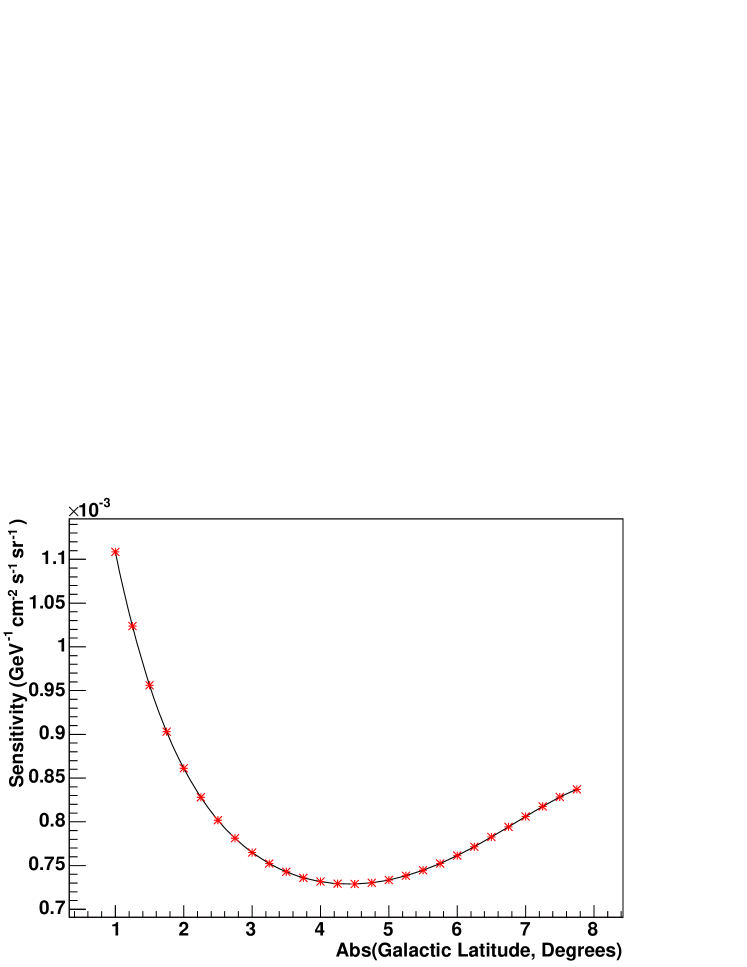
Figure 21: Sensitivity to a Gaussian source ($\sigma=2.1^{\circ}$) as a function of on-source region size.

5 Results

After unblinding the data, we observe no excess of events. We first calculate a limit on the line source flux at the 90% confidence level, and then calculate corresponding limits for diffuse and Gaussian spatial profiles using the analytical expressions above (eqns. 1 and 2). These results are presented in table 4 for a signal spectrum of $E^{-2.7}$. The energy range of these limits, incorporating the central 90% of the signal spectrum after all selection criteria, is 0.2 to 40 TeV. The calculation has been repeated using spectral slopes from -2.4 to -2.9, resulting in diffuse-flux limits ranging from $5.3\times 10^{-5}$ to $3.1\times 10^{-3}\ \mathrm{GeV}^{-1}\mathrm{cm}^{-2}\mathrm{s}^{-1}\mathrm{sr}^{-1}$.

Because the signal flux is normalized using atmospheric neutrino MC, the largest systematic error is the uncertainty of $\sim$30% on the absolute atmospheric neutrino flux, and this has been incorporated into the limits [9],[10]. Possible unquantified sources of error are variations in the width of the Gaussian signal profile, and the offset of the peak flux from the galactic equator.

On-source	On-source	Expected	Event	Line source limit	Diffuse limit	Gaussian limit
region	events	background	upper limit
$\pm 2.0^{\circ}$	128	129.4	19.8	$6.3\times 10^{-5}$	$6.6\times 10^{-4}$	–
$\pm 4.4^{\circ}$	272	283.3	20.0	–	–	$4.8\times 10^{-4}$

Table 4: Preliminary limits on the $\nu_{\mu}+\bar{\nu}_{\mu}$ flux at Earth from the outer galactic plane, for an $E^{-2.7}$ spectrum (systematic errors included). Units on the line source limit are $\mathrm{GeV}^{-1}\mathrm{cm}^{-2}\mathrm{s}^{-1}\mathrm{rad}^{-1}$; units on the other two limits are $\mathrm{GeV}^{-1}\mathrm{cm}^{-2}\mathrm{s}^{-1}\mathrm{sr}^{-1}$.

6 Conclusions

Comparing the limit for a Gaussian flux profile in table 4 with the model prediction in section 1, we find that the sensitivity of this analysis is approximately two orders of magnitude above the predicted flux. IceCube, the $\mathrm{km}^{3}$-scale successor to AMANDA-II, will have a larger effective area and better angular resolution [11]. Only for the most optimistic case, in which the source profile is nearly a line, will the increase in angular resolution allow a significantly smaller on-source window. For five years of data from the complete detector, the total improvement in sensitivity is just over one order of magnitude. Other approaches may be more sensitive – for example, we can focus only on dense areas of the ISM, such as the Cygnus region. Also, recent calculations by Candia suggest that IceCube may be sensitive to the flux from the Galactic Center using cascades from down-going neutrinos [12]. Detection of specific sources within the plane may well precede discovery of a truly diffuse flux from the galactic disk.

The Search for Neutrinos from Gamma-Ray Bursts with AMANDA

K. Kuehn^a, for the IceCube Collaboration and the IPN Collaboration
(a) Department of Physics and Astronomy, University of California Irvine, CA 92697-4575 USA Presenter: K.Kuehn (kuehn@HEP.ps.uci.edu), usa-kuehn-K-abs1-og25-oral

[The Search for Neutrinos from GRBs with AMANDA]The Search for Neutrinos from Gamma-Ray Bursts with AMANDA [K. Kuehn for the IceCube Collaboration] K. Kuehn^a, for the IceCube Collaboration and the IPN Collaboration
(a) Department of Physics and Astronomy, University of California Irvine, CA 92697-4575 USA
Presenter: K.Kuehn (kuehn@HEP.ps.uci.edu), usa-kuehn-K-abs1-og25-oral

1 Introduction

Gamma-ray bursts (GRBs) are among the most energetic phenomena in the universe. All are characterized by prodigious gamma-ray emission, hypothesized to occur as a result of the collapse of a massive star or the merger of compact objects. Aspects of these theories have been corroborated by recent observations [1, 2]; however, many questions about the nature of GRBs still remain. One of the promising techniques currently available to answer such questions is to use underwater or under-ice detectors to observe possible high-energy neutrinos from these sources [3, 4]. The search for neutrino emission will help to test models of hadronic acceleration in the fireball [3, 4, 5] or other GRB scenarios, and the search for precursor neutrinos may constrain models of GRB progenitors [6, 7]. AMANDA uses the ice at the South Pole to detect Čerenkov radiation from neutrino-induced muons from both atmospheric interactions and astrophysical sources [8], including, potentially, GRBs. In its initial configuration (AMANDA B-10, operational from 1997-1999), the detector consisted of an array of 302 photo-detectors housed in optical modules (OMs) beneath the surface of the ice cap; the upgraded configuration of 677 OMs (operational from 2000 to 2004) was known as AMANDA-II.

2 Observation and Analysis

The AMANDA GRB search relies on spatial and temporal correlations with photon observations of other instruments, such as the Burst and Transient Source Experiment [9] or the satellites of the InterPlanetary Network [10]. For each GRB, we search for coincident neutrino emission during the entire burst duration, plus the 10 seconds prior to the burst start (plus corrections associated with uncertainties in burst timing). We also perform a search for precursor neutrino emission from 110 seconds prior to the burst trigger up to 10 seconds before the trigger. To determine the expected background rate for each burst, a larger period of one hour and 50 minutes of data is analyzed – from one hour before the burst to one hour after the burst. The 10 minute period during and immediately surrounding the burst is excluded from the background region, to ensure that the data selection criteria are not chosen in a biased fashion (a ”blind analysis”). In addition, the event count per 10 second time bin during the background period is compared to the expected (temporally uncorrelated) distribution of background events. This test determines if there are significant fluctuations in data rate due to any intrinsic instability in the detector which could be misinterpreted as a signal event. All data included in the GRB searches satisfy these criteria established for stable detector operation.

The data selection criteria for the coincident and precursor searches are determined by minimizing the Model Rejection Factor [11], which is defined as the 90$\%$ event upper limit derived from observed background events divided by the expected number of signal events determined from Monte Carlo simulations of the predicted neutrino flux. For the coincident search, the predicted flux is derived from the Waxman-Bahcall model [3] (corrected for neutrino oscillations), and for the precursor search, the predicted flux is derived from the model of Razzaque $\it{et}$ $\it{al.}$ [6]. In addition to temporal coincidence, several other selection criteria were used in these analyses, including: the angular mismatch between the burst position and the reconstructed event track (based upon a maximum-likelihood pattern recognition algorithm applied to the photon arrival time at each OM), the angular resolution of the reconstructed event track, and the uniformity of the spatial distribution of the hit OMs. The detector’s effective area ($A_{eff}$) is determined after all selection criteria are applied, and provides a measure of the detector’s sensitivity to neutrino-induced muons passing through (or nearby) the detector. Though the selection criteria for the coincident and precursor searches differ slightly, both require only modest background rejection, giving AMANDA-II an $A_{eff}$ larger than any other currently-operating neutrino detector (Figure 22).

Figure 22: Angle-averaged muon effective area as a function of muon energy, utilizing the data selection criteria from the year 2000 coincident GRB search.

3 Results and Discussion

AMANDA data from 1997-2000 were searched for emission coincident with 312 bursts detected by BATSE’s online triggering system. As reported elsewhere [12], zero events were observed, which results in an observed upper limit on the muon neutrino flux of 4 $\times$ 10^-8 GeV cm^-2 s^-1 sr^-1 (assuming a Waxman-Bahcall energy spectrum). Since the time of these observations, the coincident analysis has been expanded to include bursts detected by other satellites of the InterPlanetary Network. This search for 139 BATSE + IPN bursts from 2000-2003 also resulted in zero observed events, leading to an even more stringent upper limit of 3 $\times$ 10^-8 GeV cm^-2 s^-1 sr^-1. These observations specifically exclude significant neutrino emission from GRB030329 (for a more detailed independent analysis of this unique burst, see [13]). Additionally, we searched the 2001-2003 subset of bursts for a precursor neutrino signal; no events were observed. Therefore, an upper limit of 5 $\times$ 10^-8 GeV cm^-2 s^-1 sr^-1 is derived for the precursor neutrino flux predicted by Razzaque $\it{et}$ $\it{al.}$. The observations are summarized in Table 5 and the flux upper limits are shown in Figure 24.

Table 5: Gamma-Ray Bursts Included in the AMANDA Observations

Year	$N_{Bursts}$	$N_{BG}$	$N_{0bs}$	Event U.L.	MRF	MRF (Sensitivity)
2000	88	1.02	0	1.61	9	13
2001	15	0.05	0	2.38	64	66
Precursor	15	0.06	0	2.39
2002	17	0.08	0	2.36	54	54
Precursor	17	0.06	0	2.38
2003	19	0.10	0	2.34	52	54
Precursor	18	0.06	0	2.38
00-03	139	1.25	0	1.47	5	10
Precursor	50	0.16	0	2.28

Though specific neutrino energy spectra have been assumed thus far, the results of these analyses can be applied to other energy spectra as well, by using the Green’s Function fluence method as presented by the Super-Kamiokande Collaboration [16]. By folding the energy-dependent sensitivity of the detector into a desired theoretical spectrum, one can straightforwardly derive a flux limit for that specific spectrum. The Green’s Function fluence limit for AMANDA-II (Figure 24) extends several orders of magnitude beyond the energy range of the Super-Kamiokande limit. It is also significantly (up to a factor of 10) lower compared to the Super-Kamiokande results in the overlapping energy region, primarily due to the much larger effective area of AMANDA-II.

Figure 23: Flux Limits for AMANDA-II observations (solid lines) and flux predictions for precursor and coincident spectra (dashed lines)

Figure 24: Green’s Function Fluence Limit for AMANDA-II observations of BATSE and IPN triggered bursts. Note that the Super-Kamiokande results also include non-triggered BATSE bursts.

4 Conclusions

AMANDA has searched for neutrino emission from nearly 500 GRBs based on temporal and spatial coincidence with photon detections from numerous other observatories. Thus far, zero neutrino events have been observed in correlation with these bursts. These results lead to upper limits on the fluxes that are approaching the predictions for several canonical GRB models. However, it has been observed that the individual bursts vary significantly in their expected neutrino spectra; therefore we are also constructing an analysis procedure based on more detailed models that incorporate individual burst parameters [13]. AMANDA is continuing its search for neutrino emission from various sources; even in the absence of a detection, the final results from AMANDA’s observations from 1997-2004 should result in an improvement of the flux upper limits particularly for GRBs. In February of 2005, AMANDA’s successor experiment known as IceCube [17] began operation, and its increased collecting area will allow it to swiftly improve upon the limits of its predecessor. Furthermore, the Swift satellite, operational since December 2004, is expected to localize as many as 100 additional GRBs per year [18], which will provide a significantly larger dataset for the continuing search for neutrinos from gamma-ray bursts.

5 Acknowledgements

K.Kuehn would like to thank E. Waxman and S. Razzaque for productive and thought-provoking discussions, as well as S. Desai for detailed discussions regarding the Super-Kamiokande GRB analysis.

Probing for Leptonic Signatures from GRB030329 with AMANDA-II

Michael Stamatikos^a for the IceCube Collaboration, Jenny Kurtzweil^a and Melanie J. Clarke^a
(a) Department of Physics, University of Wisconsin, Madison, 1150 University Avenue, Madison, WI 53706, USA Presenter: M. Stamatikos (michael.stamatikos@icecube.wisc.edu),  usa-stamatikos-M-abs1-og24-oral

[Probing for Leptonic Signatures from GRB030329 with AMANDA-II]Probing for Leptonic Signatures from GRB030329 with AMANDA-II

[M. Stamatikos et al.] Michael Stamatikos^a for the IceCube Collaboration, Jenny Kurtzweil^a and Melanie J. Clarke^a
(a) Department of Physics, University of Wisconsin, Madison, 1150 University Avenue, Madison, WI 53706, USA

Presenter: M. Stamatikos (michael.stamatikos@icecube.wisc.edu),  usa-stamatikos-M-abs1-og24-oral

1 Introduction

Neutrino astronomy may provide us with a new glimpse at the internal processes of gamma-ray bursts (GRBs). The Antarctic Muon and Neutrino Detector Array (AMANDA), which has been calibrated upon atmospheric neutrinos, has demonstrated the viability of high energy neutrino astronomy by using the ice at the geographic South Pole as a Cherenkov medium. Canonical fireball phenomenology [1], in the context of hadronic acceleration, predicts correlated MeV-EeV neutrinos from GRBs via various hadronic interactions [2]. Ideal for detection are TeV-PeV neutrinos in coincidence with prompt $\gamma$-ray emission, resulting in a nearly background-free search. A detailed description of the modeling techniques and an ongoing analysis featuring correlated neutrino searches of individual GRBs from the Burst and Transient Source Experiment (BATSE) are described elsewhere [3, 2]. Here, we report on a complementary search for correlated leptonic ($\nu_{\mu},\bar{\nu}_{\mu}$) emission, using models based upon the unique discrete electromagnetic characteristics and emission geometry of GRB030329, gleaned directly from satellite and ground-based observations. This represents a novel departure from searches [4] based upon a diffuse formulation [5], which utilize averaged burst parameters.

2 GRB030329: Electromagnetic Emission & The GRB-Neutrino Connection

On March 29, 2003, at $11^{\text{h}}37^{\text{m}}14.^{\text{s}}67$ (UTC), HETE-II was triggered by GRB030329 (H2652), a watershed transient which confirmed the connection between a core collapse Type Ic supernova and long duration GRB. Electromagnetic investigations of the prompt $\gamma$-ray and multi-wavelength afterglow emissions associated with GRB030329 abound in the literature (see table 6), making it a perfect specimen for study. Via forward folding deconvolution, the photon energy spectrum, was fit to the Band function [6], an empirically derived power law with smooth transition. For spectral indices $\alpha>-2$ and $\beta<-2$, the characteristic peak energy is defined as $E_{p}=[(2+\alpha)\epsilon_{\gamma}^{b}](\alpha-\beta)^{-1}$, where $\epsilon_{\gamma}^{b}$ is known as the photon break energy [6]. Hence, using standard error propagation, we find that $\epsilon_{\gamma}^{b}=115.6\pm 9.9$ keV. Doppler spectroscopy of the OT afterglow revealed a redshift measurement, which, under an assumed $\Lambda_{CDM}$ cosmology placed GRB030329 at a luminosity distance of $2.44^{+0.20}_{-0.18}\times 10^{27}$ cm. Coupled with the peak energy flux, this implies an intrinsic peak isotropic luminosity of $L_{\gamma}^{iso}\approx 5.24^{+0.86}_{-0.77}\times 10^{50}\>\text{ergs}/\text{s}$ in the 30-400 keV energy band pass. Evidence for anisotropic emission, in the form of a two component break in the afterglow spectrum, was revealed by radio calorimetry and is consistent with collimated prompt emission within a jet of opening half angle $\theta_{jet}$. This requires a beaming fraction correction, which reduces the intrinsic peak luminosity to $L_{\gamma}^{jet}=L_{\gamma}^{iso}(1-\cos\theta_{jet})\approx 1.99^{+0.33}_{-0.29}\times 10^{48}\>\text{ergs}/\text{s}$. Extended calorimetry provided an estimate for the fractions of shock energy imparted to the electrons ($\epsilon_{e}$) and magnetic field ($\epsilon_{B}$). Table 6 summarizes the observed electromagnetic properties used in this analysis.

Table 6: Electromagnetic Properties of GRB030329: Prompt $\gamma$-ray and Multi-wavelength Afterglow Emission

Parameter(s)	Value	Reference
Positional Localization $\left(\alpha_{\text{J2000}},\delta_{\text{J2000}},\sigma_{R}\right)$	$161.2081646^{\circ},21.5215106^{\circ},3.0\times 10^{-7}\>{}^{\circ}$	Taylor et al., GCN Report 2129
Trigger (T) & Duration (T90) [30-400 keV]	$41,834.67\>\text{SOD},22.8\pm 0.5\>\text{s}$	Vanderspek et al., ApJ 617: 1251-1257 (2004)
Energy Fluence ($F_{\gamma}$) [2-400 keV]	$1.630^{+0.014}_{-0.013}\times 10^{-4}\>\text{ergs}/\text{cm${}^{2}$}$	T. Sakamoto et al., astro-ph/0409128
Band Parameters $\left(\alpha,\>\beta,\>E_{p}\right)$ [2-400 keV]	$-1.32\pm 0.02$,$-2.44\pm 0.08$, $70.2\pm 2.3$	Vanderspek et al., ApJ 617: 1251-1257 (2004)
Peak Energy Flux ($\Phi_{\gamma}^{\text{Peak}}$) [30-400 keV]	$\sim 7\times 10^{-6}\>\text{ergs}/\text{cm${}^{2}$/s}$	Vanderspek et al., GCN Report 1997
Spectroscopic Redshift (z)	$0.168541\pm 0.000004$	Bloom et al., GCN Report 2212
Jet Opening Half Angle ($\theta_{jet}$)	$\sim 5^{\circ}\approx 0.09$ rad	Berger et al., Nature 426, 154-157 (2003)
Electron & Magnetic Field Energy Fractions	$\epsilon_{e}\approx 0.19$, $\epsilon_{B}\approx 0.042$	Frail et al., ApJ 619, 994-998 (2005)

The generic mechanism responsible for the super-Eddington luminosities associated with GRBs is the dissipation, via shocks, of highly relativistic kinetic energy, acquired by electrons and positrons Fermi accelerated in an optically thick, relativistically expanding plasma, commonly referred to as a fireball. The acceleration of electrons in the intense magnetic field of the fireball leads to the emission of prompt non-thermal $\gamma$-rays via synchrotron radiation. The temporal variability ($t_{v}\sim 10$ ms) in the light curves imply compact sources. In order to ensure a transparent optical depth to photons of energy $\epsilon_{\gamma}^{max}\approx 100\>\text{MeV}$, a minimum bulk Lorentz boost factor ($\Gamma$) was assigned (see equation 6). Hadronic acceleration within the ambient photon field produces TeV-PeV leptons, whose spectra $(dN_{\nu_{\mu}}/d\epsilon_{\nu_{\mu}}\equiv\Phi_{\nu_{\mu}})$ trace the photon spectra, via the following photomeson interaction: $p+\gamma\rightarrow\Delta^{+}\rightarrow\pi^{+}+[n]\rightarrow\mu^{+}+\nu_{\mu}\rightarrow e^{+}+\nu_{e}+\bar{\nu}_{\mu}+\nu_{\mu}$, as illustrated in figures 26 and 26 [3, 7]. Hence, these $\nu$s are expected to be spatially and temporally correlated with prompt $\gamma$-ray emission.

3 Neutrino Astronomy with AMANDA-II: Analysis, Results & Discussion

AMANDA-II is comprised of 677 optical modules buried at depths between 1500-2000 m. The background consists of cosmic ray induced down-going atmospheric muons, detected at a rate of $\sim 100$ Hz, with a perturbation of atmospheric neutrinos, detected at a rate of $\sim 10^{-4}$ Hz. The astrophysical neutrino signal, detected via charged current interactions such as: $\nu_{\mu}+N\rightarrow\mu^{\pm}+X$, is isolated by utilizing topologically identified up-going muon events, which are reconstructed by a maximum likelihood method. On-source, off-time data were used to estimate the stability of the background rate in order to maintain blindness, facilitating an unbiased analysis. After data filtering (see [8]), the total off-time background, excluding a 10 minute blinded window centered upon the trigger time, was consistent with a Gaussian fit and accrued $24,972\pm 158$ events over a 57,328.04 second interval, resulting in a rate of $0.436\pm 0.003$ Hz. Based upon a visual inspection of the light curve, a conservative search window of 40 seconds (beginning at $T$) was chosen. Hence, $17.44\pm 0.12$ background events ($n_{b}$) were expected on-time in AMANDA-II prior to any quality selection. Signal neutrino spectra were simulated for three models (see figure 26) by propagating a total of $\sim 440,000$ muon neutrinos ($\nu_{\mu}+\bar{\nu}_{\mu}$) from an error box in the sky defined by the spatial localization of the radio afterglow (see table 6). Event quality selection was optimized for the best limit setting and discovery potential by minimizing the model rejection factor (MRF) [9] and the model discovery factor (MDF) [10], respectively. Although multiple observables were investigated, a single criterion emerged, based upon the maximum size of the search bin radius ($\Psi$), i.e. the space angle between the reconstructed muon trajectory and the GRB’s position.

Our search, optimized for $5\sigma$ discovery (requiring 4 events within $\Psi\leq 11.3^{\circ}$), is consistent with a null signal. Upper limits, summarized with our results in table 7, do not constrain the models tested using AMANDA-II. Effective neutrino and muon areas are given in figure 28. The number of expected signal events in IceCube ($N_{s}$) for model 1 is consistent with [11], when neutrino oscillations are considered. For model 3, our results for $N_{s}$ are in agreement with [7] and [12], when one adjusts for the assumptions of [5]. Selection based upon $\Psi$ was robust across the models tested in AMANDA-II, as illustrated in figure 28. However, the MRF/MDF and hence the limit setting/discovery potential was strongly model dependent, varying by over an order of magnitude for models 1 and 3. Furthermore, using the same theoretical framework, the response of AMANDA-II and IceCube to spectra based upon discrete and average parameters are discrepant in mean neutrino energy and event rate by over an order of magnitude as illustrated in figure 26 and table 7. Such variance in detector response unequivocally demonstrates the value of a discrete modeling approach when making correlative neutrino observations of individual GRBs, especially in the context of inferred astrophysical constraints, in agreement with [7].

Table 7: Results Summary. Primes indicate value after selection. Superscripts indicate A=MRF and B=MDF optimization.

Model	$\Psi^{A},\Psi^{B}\>{}^{\circ}$	$n_{b},n_{b}^{A\prime},n_{b}^{B\prime}$	$N_{s}$, $n_{s}$, $n_{s}^{B\prime}$	$n_{obs},n_{obs}^{B\prime}$	MRF, MDF	SensitivityB, LimitB $\frac{\text{GeV}}{\text{cm${}^{2}\cdot$s}}$
1	21.3, 11.3	17.44, 0.23, 0.06	0.1308, 0.0202, 0.0156	15, 0	152, 424	0.157, 0.150
2	18.8, 11.3	17.44, 0.17, 0.06	0.0691, 0.0116, 0.0092	15, 0	256, 716	0.041, 0.039
3	18.5, 11.3	17.44, 0.17, 0.06	0.0038, 0.0008, 0.0006	15, 0	3864, 10794	0.036, 0.035

$$\epsilon_{\nu_{\mu}}^{2}\Phi_{\nu_{\mu}}\approx A_{\nu_{\mu}}\times\begin{cases}\left(\frac{\epsilon_{\nu_{\mu}}}{\epsilon_{\nu}^{b}}\right)^{-\beta-1}&\epsilon_{\nu_{\mu}}<\epsilon_{\nu}^{b}\\ \left(\frac{\epsilon_{\nu_{\mu}}}{\epsilon_{\nu}^{b}}\right)^{-\alpha-1}&\epsilon_{\nu}^{b}<\epsilon_{\nu_{\mu}}<\epsilon_{\pi}^{b}\\ \left(\frac{\epsilon_{\nu_{\mu}}}{\epsilon_{\nu}^{b}}\right)^{-\alpha-1}\left(\frac{\epsilon_{\nu_{\mu}}}{\epsilon_{\pi}^{b}}\right)^{-2}&\epsilon_{\nu_{\mu}}>\epsilon_{\pi}^{b}\end{cases}$$ (3)

$$A_{\nu_{\mu}}\approx\frac{F_{\gamma}f_{\pi}}{8\epsilon_{e}\ln(10)T_{90}}\approx 9.86\times 10^{-4}\>\text{GeV}/\text{cm${}^{2}/$s}$$ (4)

$$f_{\pi}\simeq 0.2\times\frac{L_{\gamma,52}}{\Gamma_{2.5}^{4}t_{v,-2}\epsilon_{\gamma,MeV}^{b}(1+z)}\approx 0.77$$ (5)

$$\Gamma\gtrsim 276\left[L_{\gamma,52}t_{v,-2}^{-1}\epsilon_{\gamma,MeV}^{max}(1+z)\right]^{\frac{1}{6}}\approx 178$$ (6)

$$\epsilon_{\nu}^{b}\approx\left[\dfrac{7\times 10^{5}}{(1+z)^{2}}\dfrac{\Gamma_{2.5}^{2}}{\epsilon_{\gamma,\text{MeV}}^{b}}\right]\>\text{GeV}\approx 1.40\times 10^{6}\>\text{GeV}$$ (7)

$$\epsilon_{\pi}^{b}\approx\left[\dfrac{10^{8}}{(1+z)}\epsilon_{e}^{\frac{1}{2}}\epsilon_{B}^{-\frac{1}{2}}(L_{\gamma,52})^{-\frac{1}{2}}\Gamma_{2.5}^{4}t_{v,-2}\right]\>\text{GeV}\approx 7.98\times 10^{7}\>\text{GeV}$$ (8)

Figure 25: Upper panel - Prompt neutrino energy flux for models 1 (solid black), 2 (dashed blue) and 3 (dot-dashed red), based upon equation 3. Lower panel - Detector response for models 1 (black), 2 (blue) and 3 (red) for AMANDA-II (solid) and IceCube (dashed). The effects of neutrino flavor oscillations have been included.

Figure 26: Parameterization [3, 7] of the neutrino energy spectrum. Where $L_{\gamma}\equiv L_{\gamma,52}\cdot 10^{52}\>\text{ergs/s}$, $\Gamma\equiv\Gamma_{2.5}\cdot 10^{2.5}$, $t_{v}\equiv t_{v,-2}\cdot 10\>\text{ms}$, $\epsilon_{\gamma}^{b}\equiv\epsilon_{\gamma,\text{MeV}}^{b}\cdot 1\>\text{MeV}$, and $\epsilon_{\gamma}\equiv\epsilon_{\gamma,MeV}^{max}\cdot 100\>\text{MeV}$. Values are given for model 1. Note the explicit dependence on discrete $\gamma$-ray photon observables.

Figure 27: AMANDA-II signal efficiency/background rejection for models 1-3 using MRF (vertical dashed blue, dashed-dot green and dashed-dot-dot red) and MDF (vertical black dotted) optimizations. Both MRF and MDF selections reject $\sim 99\%$ of the background while retaining $\sim 86\%$ and $\sim 77\%$ of the signal, respectively.

Figure 28: Upper panel - the effective muon neutrino area. Lower panel - the effective muon area for energy at closest approach to the detector. MDF optimized AMANDA-II results for models 1 (dashed black), 2 (dashed blue) and 3 (dot-dashed red) and predicted IceCube (solid black) curves are illustrated for $\delta_{\text{J2000}}\approx 22^{\circ}$.

Neutrino-Induced Cascades From GRBs With AMANDA-II

B. Hughey^a, I. Taboada^b for the IceCube Collaboration
(a) Physics Dept. University of Wisconsin. Madison, WI 53706, USA
(b) Physics Dept. University of California. Berkeley, CA 94720, USA

Presenter: B. Hughey (brennan.hughey@icecube.wisc.edu),  usa-hughey-B-abs1-og25-oral

[$\nu$-induced cascades from GRBs with AMANDA-II]Neutrino-Induced Cascades From GRBs With AMANDA-II [B. Hughey, I. Taboada for the IceCube Collaboration] B. Hughey^a, I. Taboada^b for the IceCube Collaboration
(a) Physics Dept. University of Wisconsin. Madison, WI 53706, USA
(b) Physics Dept. University of California. Berkeley, CA 94720, USA
Presenter: B. Hughey (brennan.hughey@icecube.wisc.edu),  usa-hughey-B-abs1-og25-oral

1 Introduction

Gamma Ray Bursts are among the most energetic processes in the universe. High energy neutrinos ($\approx 10^{14}$ eV) are thought to be produced via the process $p+\gamma\rightarrow\Delta^{+}\rightarrow\pi^{+}[+n]\rightarrow\mu^{+}+\nu_{\mu}\rightarrow e^{+}+\bar{\nu}_{e}+\nu_{\mu}$. Neutrino oscillations result in a flavor flux ratio, $\phi_{\nu_{e}+\bar{\nu}_{e}}$:$\phi_{\nu_{\mu}+\bar{\nu}_{\mu}}$:$\phi_{\nu_{\tau}+\bar{\nu}_{\tau}}$, equal to 1:1:1 at Earth. AMANDA-II, a sub-detector of IceCube, was commissioned in 2000 with a total of 677 optical modules arranged on 19 strings, at depths between 1500 m and 2000 m below the surface of the ice at the South Pole. Each OM contains a 20 cm photo-multiplier tube in a pressure vessel. AMANDA-II uses polar ice as a Cherenkov medium. Searches for $\nu$-induced muons with AMANDA-II [1, 2] in coincidence with bursts reported by satellites have been done for 1997-2003 [3]. These searches take advantage of the spatial and temporal localization of the bursts to reduce background, but are restricted to bursts with positive declination because AMANDA-II, located at the South Pole, relies on the use of the Earth to filter out all non-neutrino particles from the northern hemisphere. The cascade channel is complementary to the muon channel. AMANDA-II is uniformly sensitive to cascades from all directions, so objects at any declination can be studied. Further, GRBs without directional information can be used as no correlation to the cascade direction is required. Even though the detector’s effective volume is smaller for cascades than for muons, more bursts can be studied with the cascade channel. Isolated cascades are produced by several interactions: $\nu_{e}N$ charged current, $\nu_{x}N$ neutral current, $\bar{\nu}_{e}e^{-}$ at 6.3 PeV (Glashow resonance) and $\nu_{\tau}N$ charged current in the case when the $\tau$ travels a short distance before decaying and the decay cascade overlaps the $\nu_{\tau}N$ hadronic cascade. A 100 TeV $\tau$ will travel $O(5~{}m)$ before decaying. As a comparison, a 100 TeV electromagnetic cascade is $\approx$8.5 m long in ice.

We present two analyses that search for $\nu$-induced cascades in coincidence with GRBs. For the first analysis, hereafter referred to as the Rolling analysis, we do not use any correlation with bursts reported by satellites. Instead two time windows, 1 s and 100 s, are rolled along the data taken by AMANDA-II in the year 2001, to search for statistical excess. This technique has the advantage of being sensitive to bursts that were not reported by satellites. The second analysis, hereafter referred to as the Temporal analysis, uses the temporal, but not the spatial, correlation with bursts reported by BATSE [4] in the year 2000. Using this correlation reduces the background significantly.

2 Simulation and Reconstruction

For both analyses neutrino-induced cascades for all three neutrino flavors were simulated with ANIS [5] from 100 GeV to 100 PeV following an $E^{-1}$ spectrum. This simulation was then re-weighted to follow the flux predicted by the Waxman-Bahcall model [6]. This spectrum is derived from average burst characteristics, and thus it is adequate to describe a large number of bursts simultaneously. Individual burst spectra may deviate significantly from the WB spectrum. We use a break energy, $E_{B}$=100 TeV and a synchrotron energy, $E_{s}$=10 PeV. For the Rolling analysis signal simulation was verified with TEA [7] which produces a Waxman-Bahcall type broken power law spectrum directly. The outputs of ANIS and TEA were found to be consistent. In both the Rolling and Temporal analyses, background muon events were simulated with CORSIKA [8]. Muons were propagated through ice using MMC [9] and detector response was simulated with AMASIM [10] for both signal and background simulation.

For both analyses, data were reconstructed with 2 different hypotheses: a cascade hypothesis and a muon hypothesis. Muon and cascade reconstruction methods are described in refs. [11, 12, 13]. We obtain a cascade vertex resolution of about 6 m in the x,y coordinates and slightly better in the z coordinate. We obtain a cascade energy resolution of $\log_{10}E_{\rm true}/E_{\rm reco}\approx$ 0.15. The Rolling analysis reconstructs the position of cascades while for the Temporal analysis both the position and the energy of the cascade is reconstructed. The angular resolution of the muon reconstruction is about $5^{\circ}$ .

3 Rolling Time Window Analysis

The Rolling analysis currently uses data from the year 2001. We scan the entire data sample for a clustering of events which survive cuts and are not consistent with the expected background. Therefore, it has the potential to detect signals which are not coincident with prior gamma-ray detections. These sources include gamma-ray dark neutrino sources, such as choked GRBs [14] as well as conventional GRBs not detected by the Third Interplanetary Network (IPN3) [15]. The live-time of this analysis is $\approx$233 days. Two separate rolling searches are performed, with time window lengths of 1 and 100 seconds. These lengths were chosen, based on the bimodal plot of GRB durations produced by BATSE [16], to contain the majority of signal from short and long bursts, respectively, while still being short enough to keep out extra background events. Since there is no temporal or spatial coincidence to aid in background rejection, the use of cuts to reduce the background of atmospheric muons becomes very important. Cuts based on both topology and number of hits in optical modules (which is indirectly tied to event energy) are utilized. After an initial filter is applied to take only high energy events, a final cut is made using a support vector machine (SVM) [17]. Background muon Monte Carlo was found to be in good agreement with experimental data in all 6 variables used in the SVM. A sample of experimental data taken from 5 runs distributed throughout the year was used as background in the SVM. The SVM cut was optimized independently for the 1 second and 100 second searches. Since the background is of stochastic nature, Poisson statistics can be used to estimate the the statistical significance of a cluster of events. Preliminary calculations result in a sensitivity of $2.7\times$10^-6 GeV cm^-2 s^-1 sr^-1 for a time-averaged diffuse neutrino flux of all flavors, with energy spectrum according to the Waxman-Bahcall model. This sensitivity assumes 425 bursts during the live-time of this analysis based on the average rate of GRB detection by the BATSE experiment and does not account for the unknown number of bursts with weaker or non-existent gamma-ray signals. Final results are not yet available at the time of writing.

4 Temporal Analysis: Bursts reported by BATSE in 2000

AMANDA-II began normal operation Feb. 13, 2000. The last BATSE burst was reported May 26, 2000. In this period 76 bursts were reported. Since the GRB start time and duration, are well known, the separation of $\nu$-induced cascade signal from the down-going muon background is simplified. We use three selection criteria based on the two reconstruction hypotheses to discard the down-going muon background and keep the neutrino-induced cascade signal. A total of $\approx$7800 s per burst were studied. A period of 600 s (on-time window) centered at the start time of the GRB was initially set aside in accordance with our blind analysis procedures. Two periods of data of 1 hour duration (off-time window) just before and after the on-time window are also studied. We optimize the selection criteria using the off-time window and signal simulation. Thus the background is experimentally measured. We only examined the fraction of the on-time window corresponding to the duration of each burst. Keeping the rest of the on-time window blind allows for other future searches, e.g. precursor neutrinos. We determined the detector stability using the off-time window experimental data. Only GRBs for which the detector is found to be stable in the off-time windows were used. Of the 76 bursts reported by BATSE in coincidence with AMANDA-II, for two bursts there are gaps in the AMANDA-II data and for one burst, AMANDA-II data was found to be unstable. Figure 29 shows a sample of the plots used to determine the stability. We applied the selection criteria in two steps, a filter and final selection. The filter rejects down-going muons, $\theta_{\mu}>70^{\circ}$, and keeps events that are cascade-like, $L_{mpe}<7.8$. The parameter $L_{mpe}$ is the reduced likelihood of the cascade vertex reconstruction and has smaller values for cascade-like events. The final selection criteria are $L_{mpe}<6.9$ and $E>40$ TeV, where $E$ is the reconstructed cascade energy. One event in the off-time window remains after all cuts. This is equivalent to a background of $n_{b}=0.0054^{+0.013}_{-0.005}$ (stat) in the on-time window. After un-blinding the on-time window, no events were found. To set a limit, we assume a WB-like spectrum with $E_{b}=100$ TeV and $E_{s}=10$ PeV. We assume neutrino flavor flux ratio of 1:1:1 and p-$\gamma$ neutrino generation. The 90% c.l. limit on the all-flavor flux factor is $9.5\times$10^-7 GeV cm^-2 s^-1 sr^-1. The event upper limit is 2.44. These limits have not yet been corrected for systematic uncertainties. Once the systematic uncertainties have been taken into account this limit will worsen slightly.

Figure 29: Left - Rolling Analysis: Plots showing background stability. The upper plot shows background counts per day after the SVN cut and the lower plot shows time between events surviving cuts. The line is the prediction assuming Poissonian statistics. Right - Temporal Analysis: Stability plots for BATSE-8031. The upper panel shows the frequency of events/10s that pass the filter in the off-time window. The lower panel shows the number of events/10s that pass the filter versus time in seconds after midnight (UTC). The vertical lines indicate the off-time period. The on-time period is analyzed according to our blindness procedures.

5 Outlook and Conclusions

Two methods for searching for neutrino-induced cascades from GRBs using AMANDA-II have been presented. A Rolling Time Window search is being conducted to search for a neutrino GRB signal at any time and from any direction. This method serves as a useful complement to satellite-coincident GRB searches conducted with AMANDA-II. Its sensitivity to individual bursts suffers from the lack of temporal constraints, but it has the potential to observe neutrino signals from transients which would otherwise be missed. Although this search is currently being conducted on the 2001 data set, it is relatively straightforward to expand the search to data sets from later years. This method can also be adapted to use the muon channel in addition to cascades.

Temporal correlation with satellites was used to perform a search with very low background. No evidence for neutrinos was found and we have set a limit based on the WB flux. The 90% c.l. limit on the all-flavor flux factor, supposing 1:1:1 flavor flux ratio, is $9.5\times$10^-7 GeV cm^-2 s^-1 sr^-1. This value has not yet been corrected for systematic uncertainties. Previous searches by AMANDA-II, performed on a much larger set of bursts [3], have a significantly better sensitivity than what has been presented here. Given a large random set of bursts with both positive and negative declination, we expect the cascade channel sensitivity to be roughly half as sensitive as the muon channel. It is expected that only a small fraction of all bursts will contribute significantly an eventual observed neutrino flux. By monitoring both hemispheres we increase the probability of discovery. The Temporal Analysis can be expanded to include bursts reported by IPN3, Swift and by using newly or soon to be deployed IceCube strings.

Search for neutralino dark matter with the AMANDA neutrino detector

D. Hubert^a, A. Davour^b and C. de los Heros^b for the IceCube Collaboration
(a) Vrije Universiteit Brussel, Dienst ELEM, B-1050 Brussels, Belgium
(b) Division of High Energy Physics, Uppsala University, S-75121 Uppsala, Sweden

Presenter: D. Hubert (hubert@hep.iihe.ac.be), bel-hubert-D-abs1-he23-oral

[Search for neutralino dark matter with the AMANDA neutrino detector]Search for neutralino dark matter with the AMANDA neutrino detector [D. Hubert, A. Davour, C. de los Heros et al.] D. Hubert^a, A. Davour^b and C. de los Heros^b for the IceCube Collaboration
(a) Vrije Universiteit Brussel, Dienst ELEM, B-1050 Brussels, Belgium
(b) Division of High Energy Physics, Uppsala University, S-75121 Uppsala, Sweden
Presenter: D. Hubert (hubert@hep.iihe.ac.be), bel-hubert-D-abs1-he23-oral

1 Introduction

Cosmological observations have long suggested the presence of non-baryonic dark matter on all distance scales. The WMAP results [1] confirmed our current understanding of the Universe, summarised in the concordance model. In this model the Universe contains about 23% non-baryonic cold dark matter, but nothing is predicted about the nature of this dark matter.

A massive, weakly interacting and stable particle appears in Minimally Supersymmetric extensions to the Standard Model that assume R-parity conservation. Indeed, the supersymmetric partners of the electroweak neutral Standard Model bosons mix into an interesting dark matter candidate, the neutralino, whose mass is expected in the GeV-TeV range [2].

On their trajectory through the Universe these particles will scatter weakly on normal matter and lose energy. Eventually, the dark matter particles will be trapped in the gravitational field of heavy celestial objects, like the Earth and the Sun [3]. The particles accumulated in the center of these bodies can annihilate pairwise. The neutrinos produced in the decays of the Standard Model annihilation products can then be detected with a high energy neutrino detector as an excess over the expected atmospheric neutrino flux.

In this paper we present the results of searches with the AMANDA detector for neutralino dark matter accumulated in the Earth (1997-1999 data set) and the Sun (2001 data set). We also summarize current techniques that continue these efforts on higher statistics data samples accumulated during recent years.

The Antarctic Muon And Neutrino Detector Array [4] at the South Pole uses the polar ice cap as a Cherenkov medium for the detection of relativistic charged leptons produced in high energy neutrino interactions with nuclei. The detector was constructed between 1996 and 2000. Now totaling 677 light sensitive devices distributed on 19 strings, the detector is triggered when at least 24 detector modules are hit within a sliding 2.5$~{}\mu$s window. Before 2000, the detector configuration consisted of between 10 and 13 strings and consequently a lower multiplicity trigger condition was able to cope with the high rate of events produced by cosmic ray interactions with the atmosphere.

Reconstruction of muons, with their long range, offers the angular resolution required to reject the atmospheric background and search for a neutralino-induced signal, which, due to the geographic location of AMANDA, yields vertical upward-going (Earth) or horizontal (Sun) tracks in the instrumented volume. Indeed, it is possible to eliminate the dominant background, downward-going atmospheric muons. However, upward-going atmospheric neutrinos will always contaminate the final, selected data sample.

2 Signal and background simulation

We have used the DARKSUSY program [5] to generate dark matter induced events for seven neutralino masses between 50 GeV and 5000 GeV, and two annihilation channels for each mass: the $W^{+}W^{-}$ channel produces a hard neutrino energy spectrum ($\tau^{+}\tau^{-}$ for a 50 GeV neutralino), while $b\bar{b}$ yields a soft spectrum. The cosmic ray showers in the atmosphere, in which downward-going muons are created, are generated with CORSIKA [6] with a primary spectral index of $\gamma$=2.7 and energies between 600 GeV and 10${}^{11}~{}$GeV. The atmospheric neutrinos are produced with NUSIM [7] with energies between 10 GeV and 10${}^{8}~{}$GeV and zenith angles above 80^∘.

3 Search for neutralino annihilations in the center of the Earth

Figure 30: (a) Detection efficiencies relative to trigger level for the different filter levels in the terrestrial neutralino analysis ($m_{\chi}$=250 GeV, hard spectrum) for 1997-1999 data, neutralino signal, atmospheric muons and neutrinos. (b) As a function of neutralino mass, the 90% confidence level upper limit on the muon flux coming from hard neutralino annihilations in the center of the Earth compared to our results from 1997 data [9] and other indirect experiments [10]. Markers show predictions for cosmologically relevant MSSM models, the dots represent parameter space excluded by CDMS [11].

A neutralino-induced signal from the center of the Earth was searched for in AMANDA data collected between 1997 and 1999, with a total effective livetime of 536.3 days. To reduce the risk of experimenter bias, the complete data set of 5.0$\times$10⁹ events was divided in a 20% subsample, used for optimisation of the selection procedure, and a remaining 80% sample, on which the selection was applied and final results calculated. Similarly, the sets of simulated events were divided in two samples: the first for use in the selection optimisation and the second for the selection efficiency calculations. The simulated atmospheric muon sample contains 4.2$\times$10⁹ triggered events (equivalent to an effective livetime of 649.6 days). The sample of atmospheric neutrinos totals 1.2$\times$10⁸ events, which corresponds to 2.2$\times$10⁴ triggers when scaled to the livetime of the analysis.

First, we try to suppress the dominant atmospheric muon background which is about 10⁶ times more abundant than the atmospheric neutrino background. This is partially done by selecting the events that are reconstructed as upward-going and that satisfy a cut correlated with reconstruction quality (“filter level 3”). However, only a 10^-3 reduction of the atmospheric muons is obtained this way (Fig. 30a) and more elaborate selection criteria are needed to reject downward-going muon tracks misreconstructed as upward-going. Depending on the detector configuration and the neutralino model under study, the characteristics of the signal differ, which influences selection efficiencies significantly at this point. Therefore, all further cuts are fine-tuned separately for each neutralino model and year of data taking. At filter level 4, a neural network is trained using between 8 and 10 input observables, reaching another 10^-3 reduction. Filter level 5 cuts sequentially on observables, with the goal of removing downward-going muons that resemble signal events.

At filter level 5 the data sample is dominated by atmospheric neutrinos (see Fig. 30a). With no significant excess of vertical tracks observed, the final selection on reconstructed zenith angle (filter level 6) was optimised for the average lowest possible 90% confidence level upper limits on the muon flux. From the number of observed events and the amount of (simulated) background in the final angular search bin, we infer the 90% confidence level upper limit on the number of signal events. Combined with the effective volume at the final cut level and the livetime of the collected data, this yields an upper limit on the neutrino-to-muon conversion rate, which can then be related to the muon flux [8] (see Fig. 30b).

4 Search for neutralino annihilations in the Sun

Figure 31: (a) Detection efficiencies relative to trigger level for the different filter levels in the solar neutralino analysis ($m_{\chi}$=500 GeV, hard spectrum) for 2001 data, neutralino signal, atmospheric muons and neutrinos. (b) As a function of neutralino mass, the 90% confidence level upper limit on the muon flux coming from hard neutralino annihilations in the center of the Sun compared to other indirect experiments [10]. Markers show predictions for cosmologically relevant MSSM models, the dots represent parameter space excluded by CDMS [11].

The AMANDA data used in the search for solar neutralinos consists of 8.7$\times$10⁸ events, corresponding to 143.7 days of effective livetime, collected in 2001. In contrast to the search in Section 3, reducing the risk of experimenter bias in this analysis can be achieved by randomizing the azimuthal angles of the data. The advantage of this procedure is that it allows the use of the full data set for cut optimisation. The azimuthal angles are restored once the optimisation is finalised and results are calculated. The simulated atmospheric background sample at trigger level totals 1.6$\times$10⁸ muons (equivalent to 32.5 days of effective livetime) and 1.9$\times$10${}^{4}~{}$neutrinos.

The solar neutralino analysis suffers the same backgrounds as the terrestrial neutralinos, but the signal is expected from a direction near the horizon, due to the trajectory of the Sun at the South Pole. This analysis was only possible after completion of the AMANDA-II detector, whose 200 m diameter size provides enough lever arm for robust reconstruction of horizontal tracks.

We adopted a similar analysis strategy as in Section 3. First, we select events with well-reconstructed horizontal tracks (filter level 1-3). The remaining events are passed through a neural network that was trained separately for the neutralino models under study and used data as background (filter level 4). Although a data reduction of $\sim$10^-5 compared to trigger level is achieved, the data sample is still dominated by misreconstructed downward-going muons. As shown in Fig. 31a, they are removed with extra cuts on observables related to reconstruction quality (filter level 5).

There was no sign of a significant excess of tracks from the direction of the Sun in the final data sample. The expected background in the final search bin around the Sun was estimated from off-source data in the same declination band, which eliminates the effects of uncertainties in background simulation. Combining this with the number of observed events, the effective volume and the detector livetime, we obtain 90% confidence level limits on the muon flux coming from annihilations in the Sun for each considered neutralino mass [12], as shown in Fig. 31b.

5 Discussion and outlook

Figures 30b and 31b present the AMANDA limits on the muon flux from neutralino annihilations into $W^{+}W^{-}$ (hard channel) in the Earth and the Sun respectively, together with the results from other indirect searches. Limits have been rescaled to a common muon treshold of 1 GeV using the known energy spectrum of the neutralinos. Also shown are the cosmologically relevant MSSM models allowed (crosses) and disfavoured (dots) by the direct search from CDMS [11]. Compared to our search for a terrestrial neutralino signal in 1997 AMANDA data [9], the limit has been improved by a factor which is more than that expected from additional statistics alone. This is due mainly to the separate cut optimization for each neutralino mass, which exploits the characteristic muon energy spectrum of each model.

In 2001 an extra trigger was installed that lowered the energy threshold of the detector. This trigger takes into account spatio-temporal correlations in the event hit pattern. A preliminary analysis with data taken in 2001 and 2002 shows an improvement of a factor of about 5 in the effective volume in the search for 50 GeV neutralinos (soft annihilation channel) from the Earth with respect to the analysis presented in this note. We are currently performing searches for a dark matter signal both from the Earth and the Sun with data taken from 2000 and later. The increased detector exposure combined with improved reconstruction techniques and the new trigger setting will result in improved limits from these analyses (note that a 4-year exposure alone would already give an improvement of a factor of two).

Performance of AMANDA-II using Transient Waveform Recorders

A. Silvestri^a for the IceCube Collaboration
(a) Department of Physics and Astronomy, University of California, Irvine, CA 92697, USA

Presenter: A. Silvestri (silvestri@HEP.ps.uci.edu), usa-silvestri-A-abs1-og27-poster

[Performance of AMANDA-II using Transient Waveform Recorders]Performance of AMANDA-II using Transient Waveform Recorders [A. Silvestri for the IceCube Collaboration] A. Silvestri^a for the IceCube Collaboration
(a) Department of Physics and Astronomy, University of California, Irvine, CA 92697, USA Presenter: A. Silvestri (silvestri@HEP.ps.uci.edu), usa-silvestri-A-abs1-og27-poster

1 Description of $\mu$-DAQ and TWR-DAQ Systems in AMANDA

The Antarctic Muon And Neutrino Detector Array (AMANDA) is the first neutrino telescope constructed in transparent ice, and deployed between 1500 m and 2000 m beneath the surface of the ice at the geographic South Pole in Antarctica. AMANDA-II [1] was completed in February 2000 and has taken data routinely since that time [2]. It is designed to search for neutrinos that originate in the most violent phenomena in the observable universe. AMANDA has searched for point sources in the entire northern sky and for diffuse sources of high energy neutrinos of cosmic origin.

Since 1997 the detector is taking data using a data acquisition electronics based on Time to Digital Converters (TDC) which measures the arrival time of the PMT pulses, and Analog to Digital Converters (ADC), which record the maximum value of the PMT pulse amplitude. Limitation of this system are the TDC with a maximum of 8 leading edges per trigger, and the peak ADC that records only one amplitude per event. The limitation is particularly acute for bright, high energy events, because important information on afterpulses is lost. The data acquisition electronics of the AMANDA-II detector was upgraded in 2003 to readout the complete waveform of the photomultiplier tubes (PMTs) using Transient Waveform Recorders (TWR) [3]. Afterpulse information is crucial to extend the dynamic range of Number of photo-electron (Npe) measurement up to 5000 photons [3].

In order to distinguish the two data acquisition electronics of the AMANDA detector, we call $\mu$-DAQ the original system operating since 2000, and TWR-DAQ the upgraded system using waveforms since 2003. The decision was made to run the two systems in parallel until the TWR-DAQ was proven to work as satisfactorily. To compare the two systems the data from 2003 has been analyzed with both read-out systems. Additional information on the TWR-DAQ hardware can be found in [4].

Extending the analysis tools to include TWR data required several new developments: (1) The TWR-DAQ measures the integrated charge $\cal{Q}$ of the PMT pulses. In contrast, the $\mu$-DAQ only measures the maximum amplitude of the PMT waveform in a 2 $\mu$s window. (2) We account for various time offsets and we extract a timing resolution of few nanoseconds. The performance of the TWR-DAQ is tested by comparing the results for the absolute rate of atmospheric neutrinos and the $cos(\theta)$ distribution with the results from the standard $\mu$-DAQ.

2 Data Processing and Comparison of $\mu$-DAQ and TWR-DAQ Systems

The TWR-DAQ data volume reaches 15TB per year compared to $\sim$ 1TB of the $\mu$-DAQ system. The data information of the two systems has been merged according to GPS time and the fraction of overlapping PMTs participating in the event in both systems. For this analysis we restricted the capabilities of the TWR-DAQ system to mimic the features of the $\mu$-DAQ system as close as possible. The timing and amplitude information extracted from waveforms has been used as input parameters to perform PMT-pulse cleaning, TOT (Time-Over-Threshold) and cross-talk cleaning.

Due to small differences in threshold values, the TWR-DAQ collects $\sim$ 80% of pulses observed in the $\mu$-DAQ system. A software re-trigger was applied at lower majority ($\cal{M}=$ 19) to obtain similar rates after PMT-pulse cleaning procedures. TOT-cleaning procedures were tested using $\mu$-DAQ data, which exclude anomalous PMT-pulses which are too short or too long. The same TOT-cleaning was performed on the TWR-DAQ data, which causes a slight loss in efficiency due to the higher threshold. Cross-talk cleaning procedures were also tested using $\mu$-DAQ data, and cross-talk tables were designed according the ADC and TOT response observed in $\mu$-DAQ data. We decided to apply the same cross-talk cleaning procedures to perform a closer comparison, however small differences are expected since the $\mu$-DAQ data contains differences TOT values, and peak ADC are replaced by the integrated charge $\cal{Q}$.

Timing and amplitude calibration have been performed using a threshold algorithm which captures the leading and trailing edge of single PMT pulses, and calculate the Npe from integrated charge. Time offsets are calculated and have been applied as $t_{offset}=t_{cable}-t_{module}-t_{delay}-t_{\cal{Q}}$, where $t_{cable}$, $t_{module}$, $t_{delay}$ and $t_{\cal{Q}}$ account for cabling offset, TWR module hardware clock, stop delay of trigger response and amplitude-timing corrections, respectively. Amplitude-timing corrections are performed by fitting the leading edge versus $1/\sqrt{\cal{Q}}$, where $\cal{Q}$ is the integrated charge rather than peak ADC measurement. These measurements are then compared to the standard timing calibration of the $\mu$-DAQ.

Figure 32: (Left) Time difference between the PMT pulses recored by the two acquisition systems $\Delta t=t_{\mu}-t_{TWR}$. (Right) Calibrated amplitude normalized to 1 photo-electron (p.e.) value for $\mu$-DAQ and TWR-DAQ data. See text for details

A Gaussian fit of the distribution for $\Delta t=t_{\mu}-t_{TWR}$ yields $\sigma_{\Delta t}=4.2$ ns (Figure 32 (left)), which is dominated by the systematic error of the time jitter between independent flash ADC clocks of the TWR system. The TWR-DAQ timing calculations are relative to the values measured by the $\mu$-DAQ. The timing of the TWR-DAQ system includes two sources of jitter, both are related to a uniform window that is 10 ns in duration. This account for the $\sigma_{\Delta t}\sim 4$ ns. Amplitudes are also calibrated by extracting the number of photo-electron (Npe) detected from peak ADC of the $\mu$-DAQ and charge $\cal{Q}$ of the TWR system and normalized to 1pe amplitude. By integrating the charge from pulse in the waveform, the dynamic range of the TWR-DAQ extends to Npe $\sim 100$, to be compared to Npe $\sim 30$ of the $\mu$-DAQ. Figure 32 (right) shows the reconstructed amplitude of the TWR-DAQ compared to the $\mu$-DAQ, which indicates a stable power law distribution extending up to 100 Npe, while the $\mu$-DAQ system shows a “knee” around 10 Npe. The knee is due to the amplitude saturation of the channels with optical fibers, approximately 40% of the AMANDA readout. After cleaning, the muon track is reconstructed from the remaining information. Details on the reconstruction techniques can be found in [5]. Table 8 summarizes the passing rates from the raw data level to the final sample of atmospheric neutrinos.

Selection	TWR-DAQ	$\mu$-DAQ
Raw Sample	$1.86\times 10^{9}$	$1.86\times 10^{9}$
Level-1	$1.25\times 10^{8}$	$1.25\times 10^{8}$
Level-3	$2.56\times 10^{6}$	$1.99\times 10^{6}$
Final Sample	1112	1026

Table 8: Passing rates for increasing cut selection level for the TWR-DAQ and $\mu$-DAQ data analysis.

Figure 33: (Left) The zenith $\Delta\theta=\theta_{\mu}-\theta_{TWR}$ difference distribution between the $\mu$-DAQ and the TWR-DAQ systems, (right) the azimuthal $\Delta\phi=\phi_{\mu}-\phi_{TWR}$ difference distribution.

Figure 33 shows that the angular mismatch for the final neutrino sample, $\sigma_{\Delta\theta}~{}{\rm is}~{}0.5^{\circ}$, where $\Delta\theta=\theta_{\mu}-\theta_{TWR}$. This value is expected from studies of the precision of the global minimizer in the reconstruction program. From the analysis based on TWR-DAQ data, 1112 neutrinos are observed compared to 1026 neutrinos from the $\mu$-DAQ data analysis. The small differences in the event rate are compatible with the small differences in analysis procedures described in Section 2.

Figure 34 shows the cos$\theta$ distribution of the atmospheric neutrino sample extracted from the TWR-DAQ and $\mu$-DAQ data analysis. Satisfactory agreement can be seen for the cos$\theta$ distribution of the atmospheric neutrinos samples obtained by the different analyses.

Figure 34: cos$\theta$ distribution after final cut level representing the atmospheric neutrino sample observed from the TWR-DAQ and the $\mu$-DAQ analyses.

3 Discussion and Conclusion

The atmospheric neutrino analysis provides the first detailed evaluation of the performance of the TWR-DAQ system. The preceding discussion demonstrated that the TWR-DAQ produces similar event rates and angular distribution as the data collected by the standard $\mu$-DAQ system. This encouraging result was obtained by first converting the waveforms into the more restricted information collected by the $\mu$-DAQ. At that point, the standard AMANDA analysis tools were applied to data from both of the electronic systems, although some of the procedures were reformulated to process waveform information.

We are developing new software tools to exploit the full information contained in the waveform. We expect that the additional information will improve energy and angular resolution crucial for the search of high energy phenomena.

4 Acknowledgements

The author acknowledges support from the U.S. National Science Foundation Physics Division, the NSF-supported TeraGrid systems at the San Diego Supercomputer Center (SDSC), and the National Center for Supercomputing Applications (NCSA).

A software trigger for the AMANDA neutrino detector

T. Messarius^a for the IceCube Collaboration (a) University of Dortmund, Otto-Hahn-Str. 4, 44221 Dortmund, Germany

Presenter: T. Messarius (messarius@physik.uni-dortmund.de),  ger-messarius-T-abs1-og27-oral

[A software trigger for the AMANDA neutrino detector]A software trigger for the AMANDA neutrino detector [T. Messarius for the IceCube Collaboration]T. Messarius^a for the IceCube Collaboration
(a) University of Dortmund, Otto-Hahn-Str. 4, 44221 Dortmund, Germany

Presenter: T. Messarius (messarius@physik.uni-dortmund.de),  ger-messarius-T-abs1-og27-oral

1 Introduction

Figure 35: Amanda II.

Since construction first began in 1996, the Antarctic Muon And Neutrino Detector Array (AMANDA) has detected high energy muons and neutrinos. Neutrinos are observed indirectly by measuring the Cherenkov light from secondary leptons generated in neutrino-nucleon interactions. AMANDA uses the ice sheet at the geographical South Pole as its active volume and consists of 19 strings of Optical Modules (OM) each containing a photomultiplier tube (PMT) and electronics in a glass sphere. Most of the 677 OMs of the detector are located at a depth of 1.5 to 2 km below the ice surface. The detector is displayed schematically in Fig. 35.

The analog PMT signals are transmitted via electrical cables or optical fibers to the surface electronics. For the reconstruction of the energy and direction of the particles, the arrival times of the pulses and the number of photons contained in each PMT pulse are used.

The original Data Acquisition system ($\mu$-DAQ) is triggered by a hardware based trigger logic, the DMADD, which identifies events through a pre-set global multiplicity condition:, i.e., more than M OMs with a signal in a 2.5 $\mu$sec time window. At low multiplicities, random coincidence of PMT noise pulses (”noise events”) dominate the muon signal. Lower multiplicity signals are triggered by local coincidence on a single string (”string trigger”).

AMANDA has produced scientific results for many years and is a working neutrino detector [1, 2].

2 The new TWR-DAQ system and science goals

The $\mu$-DAQ system uses TDCs and peak sensing ADCs to extract information from an analog PMT pulse. It uses the DMADD trigger logic with a multiplicity M=24 which results in a trigger rate of $\sim 100$ Hz. The vast majority of these triggered events are due to atmospheric muons. The settings are a compromise between the energy threshold and deadtime of the detector. This and other limitations [3, 6] of the $\mu$-DAQ led to the development of a new DAQ system based on Transient Waveform Recorders [4] (TWR), which are flash ADCs (FADC) capable of recording the complete waveform of a PMT in a time window of 10.24 $\mu$sec with a resolution of 12 bit and a sampling frequency of 100 MHz. The new system - TWR-DAQ - has a significantly lower dead time (approx 0.015%) compared to the $\mu$-DAQ system (15% deadtime), and a better readout performance leading to a higher data bandwidth. Since Feb 2003, the TWR-DAQ used the DMADD as a trigger source. In 2003, a M=24 level was used while in 2004 the trigger multiplicity was lowered to M=18 with a corresponding trigger rate of $\sim$140Hz. The $\mu$-DAQ still uses a M=24 multiplicity level. For each PMT pulse, the whole waveform is written out resulting in a larger amount of data compared to the $\mu$-DAQ system. A first reduction is performed by a Digital Signal Processor (DSP) collecting the data from the TWRs in each crate and performing a so called Feature Extraction (FE) to extract the rather short PMT pulses from the waveform. The new TWR-DAQ system is running and taking data continuously for two years [3]. In 2003 and 2004, the system produced a data rate of $\sim$65 GB per day, nearly exceeding the capability of network communication at the South Pole. For a further extension of the capabilities of the detector with respect to the intended integration of AMANDA into the IceCube detector [7, 8], the TWR-DAQ will be further upgraded. The goals for the next upgrade are:

• to reduce the energy threshold of the detector in order to increase the sensitivity for low energy particles,

• to introduce fast algorithms to search for patterns, i.e. local coincidences, in low multiplicity events to distinguish reconstructable events from noise events, and,

• to send trigger signals to the IceCube trigger system in order to integrate AMANDA into the IceCube detector.

Figure 36: Structure of the AMANDA DAQ system in 2005.

These goals can be achieved by implementing software trigger algorithms into the TWR-DAQ system. The layout of the trigger system is displayed in Fig. 36. The DMADD system is still used as a pre-trigger with a low multiplicity threshold. The global multiplicity level can be lowered from M=18 to M=12. Events with a multiplicity of M$>$18 are directly written to disk, while the remaining events are tested for local coincidences in software. The algorithm is described in the next section. A total trigger rate of $\sim$195 Hz is reached and noise events are mostly rejected. During the last update of the TWR-DAQ in January 2005 an online monitoring was implemented to the TWR-DAQ. Changes in the trigger rates and noise rates of each PMT can be monitored for each file.

3 Performance of the new TWR-DAQ system including the software trigger

The TWR-DAQ including the software trigger is running stably since mid - February 2005. Particles with high energy (100 GeV to TeV range) produce a sufficient amount of light in the detector to be triggered reliably by the DMADD multiplicity trigger while the detection efficiency for smaller energies is low. One challenge for the software trigger is an improvement of the sensitivity of the array for low energy particles by distinguishing between noise induced and particle induced events. The PMT pulses of particle induced events are correlated in time and space. A dedicated trigger algorithm searching for local coincidences identifies these events in the detector. The so-called next neighborhood algorithm (NEXT) measures the level of local coincidence in the event. For each OM with a pulse, a sphere of 90 m radius around the OM is searched for further OMs with a pulse. If there is at least one additional OM with a pulse, the number of modules with at least one local coincidence pair $N_{1hit}$ is increased by 1. Alternatively, the number of local coincidence pairs is counted in $N_{pair}$. Double counts are excluded in these numbers. In 2005, the software trigger uses $N_{pair}>8$ or $N_{1hit}>5$ to trigger event readout.
While muons produce long tracks in the detector, electrons and taus will lose their energy contained in a small volume inside the detector producing a cascade like event. Figure 37 shows that the NEXT trigger is sensitive to both of the event types.

The pre-trigger rate from the DMADD is $\sim$250 Hz. First, multiplicity (M=18) events are written to disk and excluded from further processing. The software trigger keeps about 50% of the remaining events. The distribution of the number of PMT pulses in the triggered event, $N_{hit}$ , are shown in Fig. 38. For this analysis a set of random data was taken using a frequency generator as trigger. Since the frequency generator is not correlated to any physical events the data can be used to investigate the trigger settings without any pre-trigger thresholds. At small $N_{hit}$ ($N_{hit}<25$) the distribution of the random data is dominated by Poissonian noise events. At $N_{hit}>25$ the distribution is dominated by the slowly decreasing contribution of $\mu$-events. The NEXT trigger filters at small $N_{hit}$ down to $N_{hit}=12$ the reconstructable  events out of the event stream leading to an increase of low-energy events.

Figure 37: 2D schematic of the functionality of the next neighborhood trigger. The red/gray lines between the OMs show counted pairs of hit OMs. The left picture shows a track like event, the right picture a cascade like event. The black circles show the search volume.

The dotted line in Fig. 38 shows the distribution of reconstructable events. At $N_{hit}>24$ the percentage of reconstructable events is about 90% to 100%. It decreases to $\sim$50% for $N_{hit}=16$ and is down to $\sim$15% for $N_{hit}\leq 14$.
The update of the TWR-DAQ would result in an increase of the data volume to $\sim$95 GB/day. To decrease the data volume an online compression, based on the Huffman algorithm, is used. The performance of this algorithm depends strongly on the distribution of values in the uncompressed data. In order to improve the performance of the compression, a linear prediction of the waveform values is used. Only the difference between the true value and the prediction is stored. These steps reduce the data volume to 35 GB/day. Compared to 2004, the average number of bytes per event decreased by 50% while the trigger rate increased by 40%.

4 Integration of AMANDA into IceCube

The existing AMANDA-II detector will be incorporated into the IceCube detector, which is currently under construction. The first IceCube string was installed in the ice in Jan 2005 and additional strings are planned for the next deployment season (Nov. 2005 -Feb. 2006).With the AMANDA TWR-DAQ system it is more straigthforward to integrate information from the AMANDA strings into the IceCube trigger and data formats. After the succsessful completion of the integration of the TWR-DAQ with the IceCube DAQ, the original AMANDA DAQ will be decomissioned. The AMANDA and IceCube strings will be synchronized via a common GPS clock. The TWR-DAQ will send its trigger information to IceCube Global Trigger (GT), which identifies physical events in the data stream with a software trigger algorithm. The TWR-DAQ sends its trigger information via TCP/IP to GT which handles the triggers from the IceCube sub-detectors. The IceCube DAQ is based on a custom IP-like communication with the DOMs (Digital Optical Modules). There can be a latency of several 100 milliseconds before the signals from the DOMs reach the surface. Once all sub-detectors have produced and send their own triggers to the GT, the GT orders them in time and then starts producing higher triggers which are sent to the IceCube event builder (EB). Upon receipt of the triggers from the GT, the EB requests and reads raw data including waveform information from the string processors (SP) which can hold raw data for about 30 seconds. Due to the different DAQ and Trigger architecture, only the trigger information from the TWR-DAQ will be sent to IceCube GT but not vice versa. Both data streams will be combined offline at the South Pole or in the northern hemisphere.

5 Outlook

Figure 38: The distribution of $N_{hit}$. The solid line shows the triggered data with the NEXT trigger and the global multiplicity. The dotted line shows the reconstructable events and the dashed line shows the triggered events of the year 2004 as comparison. The dash-dotted line represents $N_{hit}$ distribution obtained from random data.

The new software trigger and a future implementation of the hardware string trigger as a pre-trigger gives a great opportunity to lower the energy threshold for several analyses as well as increasing the sensitivity due to the 40% gain in trigger rate. It is intended to implement further filter algorithms to flag events containing down-going $\mu$ tracks to accelerate an offline analysis. A further idea is to implement a compensation for the cable delays of the detector to be able to reduce the time window and multiplicity level for a trigger decision. The TWR-DAQ system will be equipped with a special Gamma Ray Burst (GRB) trigger. A GRB trigger will be send from the GCN network and will be received via satellite at the Pole. As soon as a GRB alert arrived, the TWR-DAQ will store all data in the buffer and all the subsequent data for several hours.

Air showers with IceCube: First Engineering Data

T.K. Gaisser^a, for the IceCube Collaboration^b
(a) Bartol Research Institute, University of Delaware, Newark, DE USA
(b) Members of the IceCube Collaboration are listed in the appendix to the Proceedings

Presenter: T.K. Gaisser (gaisser@bartol.udel.edu),  usa-gaisser-TK-abs1-he15-oral

[Air showers with IceCube …] Air showers with IceCube: First Engineering Data [T.K. Gaisser for the IceCube Collaboration] T.K. Gaisser^a, for the IceCube Collaboration^b
(a) Bartol Research Institute, University of Delaware, Newark, DE USA
(b) Members of the IceCube Collaboration are listed in the appendix to the Proceedings Presenter: T.K. Gaisser (gaisser@bartol.udel.edu),  usa-gaisser-TK-abs1-he15-oral

1 Introduction

The IceTop km² air shower array of 80 pairs of ice Cherenkov tanks is an integral part of the design of the IceCube neutrino telescope at the South Pole. The neutrino telescope will consist of 80 strings, each instrumented with 60 digital optical modules (DOMs) between 1450 and 2450 m depth. Thus IceCube will be a three-dimensional air shower detector as well as a neutrino telescope. The power of a surface array for calibration and background studies for the neutrino telescope, as well as the physics potential for cosmic-ray studies of the combined detector, are described in Ref. [1]. At ultra-high energy, where the Earth is opaque to neutrinos from below, the surface array will give IceCube a significant ability to discriminate between downward or horizontal neutrinos and cosmic-ray induced background. With the full detector we anticipate study of the primary composition to EeV energies where the transition from galactic to extra-galactic cosmic rays may occur.

Figure 39: Map of IceTop and SPASE in 2005. The peak in the distribution of time differences between IceTop and SPASE triggers contains events seen by both arrays.

Deployment of IceCube at the Amundsen-Scott South Pole Station began in the 2004/2005 Austral summer season with the installation of one string of 60 DOMs in the deep ice and four IceTop stations on the surface. Fig. 39 shows the configuration of the first four stations relative to the existing South Pole Air Shower Experiment (SPASE) [2], which is still in operation. In this paper we present engineering data from the first four surface stations of IceCube, including coincidences with SPASE. Initial data from the deep string, including coincidences between surface and deep detectors, are presented separately [3].

2 The IceTop Array

Figure 40: Diagram of an IceTop station.

Each pair of IceTop tanks is associated with an IceCube string. The result is a surface array in a triangular pattern with a grid spacing of approximately 125 m. Each IceTop station consists of two ice Cherenkov tanks separated by 10 meters, as shown schematically in Fig. 40. The two DOMs in each tank face downward and respond primarily to light reflected from the diffusely reflecting, white liner of the tank. The ice surface is in contact with granulated insulation, so that the top inner surface is partially reflecting. The tanks are cylindrical with surface area $2.7\,{\rm m}^{2}$ and ice thickness 90 cm.

Operation of the DOMs (which is described in more detail in [3]) is controlled by digital electronics, which can be set remotely. The tanks currently operate with one DOM set at low gain ($5\times 10^{5}$) and one at high gain ($5\times 10^{6}$). Three channels of the analog transient waveform digitizer (ATWD) on the DOM main board sample the waveforms at 3.3 ns with different amplification, for a dynamic range of more than 5000.

The rate of events detected per tank depends on trigger and threshold settings. The amplitude threshold is currently set at a voltage corresponding to ten times the peak voltage of a single photo-electron. At this threshold and with no coincidence requirement, the rate per DOM is about 3 kHz. This rate includes approximately 1 kHz of muons. Simulations [4] show that the balance is due primarily to low energy electrons and to gamma-rays converting in the tank. The characteristic shape of the spectrum of single hits, which has a prominent muon peak, is shown in the left plot of Fig. 41.

For comparison with the air shower waveform shown below in Fig. 42, we also show in Fig. 41 the average waveform of a throughgoing muon in a high-gain DOM. This is obtained by averaging over a sample of waveforms corresponding to events in the muon peak of the distribution of signals shown on the left panel of Fig. 41. With 90 cm of ice thickness, typical energy-deposition by throughgoing muons is 160 to 200 MeV, depending on zenith angle. Comparison of integrated single photo-electron waveforms with the integral of the average muon waveform allows us to estimate that the typical through-going muon produces enough light to generate approximately 160 photo-electrons in the photomultiplier. The data shown in Fig. 41 were taken during initial fast calibration runs at the South Pole in January. High statistics calibration runs currently underway will provide the basis for detailed calibration of amplitude and integrated charge. Periodic sampling of the single tank spectra will also serve to monitor performance of each tank. In addition, calibration runs with events tagged by a muon telescope are planned for next season.

Figure 41: Left: Peak amplitudes of single-tank signals showing a muon peak (high-gain DOM); right: average $\mu$ waveform.

The spacing between detectors at a station is chosen so that a coincidence of two tanks at a station without hits in adjacent stations corresponds to small showers from cosmic-ray protons with primary energies in the few to ten TeV range. Such events have a high probability of producing only one muon that reaches the deep detector. Tagging such events will be useful for understanding the principal background of atmospheric muons in the deep detector.

3 Air Showers in IceTop

For a series of runs taken February through May of 2005 the IceTop trigger was set to require 10 DOMs above threshold within 2 $\mu sec$. During these initial runs there was a local coincidence requirement within a station such that a DOM only reported if at least one of the DOMs in the other tank at the station was hit. With this setup, only air showers with at least three stations reporting were recorded. The rate of air showers with this trigger is $0.7$ Hz, divided approximately 60/40 between 3-station events and 4-station events. This rate is consistent with the expected threshold of 300 TeV and is due to events in the PeV and sub-PeV energy range.

With only 4 stations, most triggers are from air showers with cores outside the perimeter of the array, and the core locations cannot therefore be determined. External events typically have one station with a much bigger signal than the others. Events with cores inside the array will display a more symmetric pattern. Fig. 42 shows a waveform display for one such “contained” event. In this figure the upper row shows the high-gain DOMs and the lower row the low-gain DOMs. Solid lines show tank A and broken lines tank B at each station. Successive panels (from left to right) show the event passing across the array from station 30 to 29. Low-gain waveforms generally track the high-gain waveforms. Shower-front fluctuations can cause significant differences between tanks at the same station (e.g. 39), and details of particle location and DOM response within a tank also cause differences. When all high-gain channels saturate, the low-gain channels may be used to extend the dynamic range of the tank response to beyond that achievable with the three ATWD channels. We expect an overall dynamic range for the tank response of approximately $10^{5}$.

Figure 42: Waveforms for a 16-fold event with a reconstructed zenith angle of 23^∘.

Off-line we can find coincidences with the SPASE array by matching up GPS times, as shown in Fig. 39b. The rate of coincidences between IceTop and SPASE triggers is about 1 per minute, which corresponds to showers in the 10 PeV range.

4 Conclusion

The four IceTop stations are recording air shower data. During the remainder of this season, tank calibration will be performed using the muon peak in the spectrum of inclusive single tank hits. In addition, fluctuations in the shower front will be studied by comparing signals in tanks at the same station, and detector fluctuations will be studied by comparing DOMs set to the same gain in one tank.

The plan for the coming season at the South Pole is to deploy 12 additional stations grid north of the present array. The result will be a 16 station air shower array with an enclosed area of $0.12\;{\rm km}^{2}$. For operation during 2006 we therefore expect to cover a range of primary cosmic-ray energies from 300 TeV to 100 PeV. Approximately 10% of IceTop triggers will also give hits in the deep detectors, giving a significant potential for calibration of the neutrino telescope with the surface array, as well initial analysis of composition in the knee region of the primary cosmic-ray spectrum.

IceCube: Initial Performance

D. Chirkin^a for the IceCube Collaboration
(a) Lawrence Berkeley National Lab Berkeley, CA 94720-8158, U.S.A.

Presenter: D. Chirkin (dchirkin@lbl.gov),  usa-chirkin-D-abs1-he15-oral

[IceCube: initial performance]IceCube: Initial Performance [D. Chirkin for the IceCube Collaboration] D. Chirkin^a for the IceCube Collaboration
(a) Lawrence Berkeley National Lab Berkeley, CA 94720-8158, U.S.A. Presenter: D. Chirkin (dchirkin@lbl.gov),  usa-chirkin-D-abs1-he15-oral

1 Introduction

Figure 43: IceCube event

The IceCube neutrino observatory at the South Pole will consist of 4800 optical sensors - digital optical modules (DOMs), installed on 80 strings between the depths of 1450 to 2450 meters in the antarctic ice, and 320 sensors deployed in 160 IceTop tanks on the ice surface directly above the strings. Each sensor consists of a 10 in. photomultiplier tube, connected to a waveform-recording data acquisition circuit capable of resolving pulses with sub-nanosecond precision and having a dynamic range of at least 250 photoelectrons per 10 ns. This year 76 such sensors were installed as a first part of the IceCube and IceTop [1] arrays.

After a sensor acquires and digitizes an event trace, it transmits the data to the surface electronics. The events are time-stamped locally with an internal (to each sensor) clock, which has an estimated drift time of $\sim 1$ ns/s. All of the DOM clocks are time-calibrated with a special procedure, which involves sending an analog pulse from the surface to the DOM, where this pulse is received, digitized, and recorded. A similar analog pulse is sent from the DOM to the surface, where it is, in turn, digitized, and analyzed together with the pulse recorded by the DOM (which is transmitted to the surface digitally after the main “round trip” calibration procedure finishes). In this report we demonstrate that events are time-stamped with a nanosecond-scale precision over the network of 76 deployed DOMs.

Fig. 43 shows an event involving all 76 DOMs. The circle size is proportional to the signal amplitude, while the color (from blue to red) indicates relative times of the hits recorded in the DOMs. All hits are consistent with an air shower on the surface coincident with a deep-ice muon, traveling down at a zenith angle of $3\pm 2^{\circ}$.

From the ice scattering-length profile shown next to the detector string, one sees that most of the detector is located in very clear ice. In fact, the lower 25 DOMs are in ice that is up to 2 times clearer than that available to the AMANDA [2] sensors located at depths of 1500-2000 meters.

2 Time resolution and muon track reconstruction

As a part of each sensor’s time calibration, round trip times of the time calibration pulses are measured (Fig. 47). The times are larger for progressively deeper sensors on the string (DOMs with numbers 1-60), and are essentially the same for the IceTop sensors (shown as DOMs with numbers 61-76). Calibrations are done automatically every few seconds. The round trip time varies slightly from one calibration to the next, and the size of the variation provides the basic measurement of the precision of the time calibration procedure (Fig. 47).

Figure 44: Round trip time of the time calibration pulse (IceTop DOMs are shown with numbers 61-76)		Figure 45: The rms resolution of the round trip time of the time calibration pulse

Figure 46: Hit time difference between 2 DOMs directly above the one flashing in clear ice		Figure 47: Hit time resolution measured with flashers for 15 DOMs on the IceCube string

Each DOM contains an array of photodiode “flashers”, which can be used for many types of calibrations. We used these to find the differences between the photon arrival times at a few DOMs directly above the ones flashing. Fig. 47 shows the distribution of such a difference for DOMs 59 and 58, when DOM 60 was flashing. The rms values for several such DOMs are shown in Fig. 47 and are best ($\sim 2$ ns) for the DOMs located in clearer ice.

Figure 48: Captured hit event waveform

A typical waveform captured by an IceCube sensor is shown in Fig. 48. The waveforms are described very well by a waveform decomposition procedure, which yields single photon hit times.

A likelihood minimization algorithm for one-string track reconstruction in multi-layered ice was used to reconstruct the deep-ice data. The scattering and absorption values used were those measured with AMANDA and extrapolated to deeper ice using available ice core data and data collected by a dust measuring device used during the string deployment.

The track-fitting algorithm was tested on a simulated data sample of downgoing muons (Fig. 52) and was found to reconstruct it rather well (Fig. 52). The rms resolution of the muon track zenith angle reconstruction is 9.7^∘ with an event hit multiplicity of 8 or more. The resolution improves rapidly as the multiplicity increases (3.0^∘ at multiplicity 20, and 1.6^∘ at multiplicity 40). This is similar to the one-string AMANDA analysis results [3].

Figure 49: Zenith angle distribution of simulated downgoing muons (red) vs. reconstructed tracks (green)		Figure 50: Zenith angle difference distribution of reconstructed and simulated tracks

Figure 51: Muon hit multiplicity distribution of data and simulation		Figure 52: Muon zenith angle distribution of data and simulation

Fig. 52 compares the hit multiplicity distribution for 8 hours of data and a similar amount of simulated data. The zenith angle distribution of the reconstructed tracks in data is compared to the simulated data in Fig. 52. The simulated data used in Fig. 52-52 was produced with standard AMANDA simulation, which was not tuned to the somewhat different trigger logic, ice conditions and different sensors of the deeper IceCube string. As the IceCube simulation matures, the apparent discrepancy observed in Fig. 52 is expected to become smaller.

Coincident deep-ice and IceTop events with a combined hit multiplicity of at least 14+14 hits collected during March, April, and May were reconstructed with both the IceTop shower reconstruction and the one-string muon track reconstruction discussed above. The resulting zenith angle distributions are compared in Fig. 56. The directions obtained with the string reconstruction seem to be systematically closer to the vertical, which may indicate the need to improve the likelihood parameterization used in the track reconstruction. Alternatively it may be due to the shower front being curved and muons originating from a different part of the shower than that seen by IceTop. We measure a systematic offset of 2.1^∘ with an rms deviation of 4.1^∘ (Fig. 56).

To measure systematic time offsets in the IceCube string we applied the one-string reconstruction to one day’s worth of data 60 times. Each of the 60 DOMs was removed once during the reconstruction, and the time residuals of the hits in those DOMs to the expected direct (unscattered) hit times from the reconstructed tracks were evaluated. The residual time distributions are consistent with the expected distribution of hits coming from nearby muons (Fig. 56). The maxima of such distributions indicate the time residuals of the most probable (in the current setup, direct) hits. In addition to systematic time calibration offsets these can be systematically removed from zero due to features of the DOM geometry still unaccounted for and scattering affecting photon propagation even at small distances. Most of these residuals are within 3 ns of each other, except for DOMs 35-43, which are located in dustier ice (Fig. 56). This indicates that the DOM clock times for the whole array (currently 76 DOMs) are calibrated to within 3 ns of each other. An apparent large time offset of DOM 60 is currently under investigation.

Figure 53: Zenith angle distribution of string-reconstructed tracks (blue) and IceTop-reconstructed coincident showers (red)		Figure 54: Zenith angle difference distribution between string-reconstructed tracks and IceTop-reconstructed coincident showers

Figure 55: Distribution of time residuals between the hits recorded by a DOM and time expectation for direct (unscattered) hits from nearby tracks reconstructed with the rest of the string		Figure 56: Distribution of direct hit time residuals for all DOMs on the deployed IceCube string

3 Conclusions

We have demonstrated that the newly deployed IceCube string is capable of detecting muons and muons coincident with IceTop air showers. The observed muon flux is compatible with the expectation from the simulation. The global detector time calibration uncertainty is 3 ns, which is better than the design requirement of 7 ns.

Calibration and characterization of photomultiplier tubes
of the IceCube neutrino detector

H. Miyamoto^a for the IceCube collaboration
(a) Dept. of Physics, Chiba University, Chiba 263-8522 Japan

Presenter: H. Miyamoto (miya@hepburn.s.chiba-u.ac.jp),  jap-miyamoto-H-abs1-og25-poster

[IceCube PMT calibration …] Calibration and characterization of photomultiplier tubes
of the IceCube neutrino detector

[H. Miyamoto for the IceCube Collaboration] H. Miyamoto^a for the IceCube collaboration
(a) Dept. of Physics, Chiba University, Chiba 263-8522 Japan Presenter: H. Miyamoto (miya@hepburn.s.chiba-u.ac.jp),  jap-miyamoto-H-abs1-og25-poster

1 Introduction

IceCube[1] is a high energy cosmic neutrino detector which will instrument a cubic kilometer of ice sheet covering the South Pole. The InIce DOMs will be deployed on eighty strings of sixty DOMs each, and these strings will be regularly spaced by 125 m over an area of approximately one square kilometer, with the DOMs at depths ranging from 1.4 km to 2.4 km below the ice surface. An IceCube event consists of Cherenkov photon profiles recorded in individual DOMs in the form of digitized waveform output from the PMT. An accurate understanding of the PMT response is, therefore, necessary in order to determine both the geometry of these events as well as to reconstruct their energies. Moreover, having carefully calibrated PMTs would lead to a significant reduction of systematic uncertainties because it is of great help in characterizing the optical properties of glacial ice more accurately. In this paper we describe our relative and absolute calibration of the IceCube PMTs. Their charge responses and photon detection efficiencies are measured and implemented in the detector Monte Carlo simulation.

2 The IceCube Optical Detector: DOM

Each DOM contains a 10 inch diameter PMT supported by coupling gel, a signal processing electronics board, an LED flasher board for calibration, and a high voltage base which powers the PMT, all of which are housed in a glass pressure sphere. It contains its own processor, memory, flash file system, and real-time operating system. Its new digital technology enables it to schedule communications in the background while acquiring data, to invoke all calibration functions under software control, and most notably, to digitize the PMT pulse and store the full waveform information.

The IceCube PMT is the Hamamatsu R7081-02 with 10 dynodes. This PMT exhibits excellent charge resolution and low noise. The PMTs in InIce DOMs are operated nominally at a gain of $\sim 1\times 10^{7}$. They exhibit an excellent peak to valley ratio ($\geq 2.0$) and remarkably low dark count rate ($\sim 500Hz$) at sub-freezing temperatures, both of which have a significant impact on the performance of the IceCube detector.

3 Fundamental PMT calibration in a freezer

The basic behavior of the PMTs at sub-freezing temperatures should be well understood. A PMT put in a freezer box is illuminated by diffuse light from a UV LED for measuring the PMT gain, single photoelectron (SPE) response, and dark count rate. An SPE waveform has been found to be represented well by a gaussian with $\sigma\sim 2$ nsec. Dark count rates above a trigger threshold of 0.3 PE were found to be distributed around $600$ Hz for PMTs with a gain of $5\times 10^{7}$. This corresponds to $\sim 470$ Hz at the operating gain of $1\times 10^{7}$.

Figure 57: Left panel:The charge histogram with the fitted SPE model function. Right panel:PMT linearity data. The output charge is plotted as a function of the number of photoelectrons corresponding to the LED luminosity. The PMT gain is $1.2\times 10^{7}$.

The charge response for SPE detection has been extensively studied. In general it is assumed that the charge of an SPE pulse follows a gaussian distribution. However, a large PMT like those used in IceCube is occasionally observed to fail to stream secondary electrons out from the first to the second dynode, which results in a non-gaussian response. Here the charge response of the IceCube PMTs is modeled by an exponential term in conjunction with the widely-used gaussian term. The left panel of figure 57 illustrates how well this model function represents the charge histogram. One of the advantages in this model representation is that the scaling law to PMT gain appears valid in the model function. The relevant model parameters are recorded into a database, which is used by the detector Monte Carlo simulation.

It is also important to measure the linearity of the PMT response to multiple photoelectrons. A bright LED with a set of calibrated neutral density filters is used to provide various luminosities of UV photons for such a linearity measurement. The result is shown in the right panel of Figure 57. The number of photoelectrons is estimated from the SPE peak and the attenuation factor of each filter. It is found that an IceCube PMT has a linear response up to approximately one thousand photoelectrons at the gain of $\sim 1\times 10^{7}$. Since a representative FWHM of the LED light pulse is 30 nsec in this measurement, the corresponding current where the PMT deviates from the linear response is $\sim 60$ mA.

4 Two dimensional photocathode scan

The IceCube PMT collects photoelectrons generated in its relatively large cathode area and its efficiency depends on the position on the cathode surface. Moreover, the variance of the electric field inside the tube to collect photoelectrons at the dynode gives non-negligible differences in the charge collection efficiency from tube to tube. We have systematically analyzed the dependency of the overall PMT efficiency on the photocathode position, using a two dimensional scan system. A UV LED moves along the curved PMT surface to scan the entire photocathode. The light beam is controlled to be precisely perpendicular to the cathode glass. A collimator attached in front of the LED gives a spot size of $\sim$1 mm. The light spot pointing accuracy is $\leq$ 4.8 mm which is sufficient to scan the cathode with its radius of $\sim$ 14 cm.

Figure 58: Left and middle panels: Examples of the position dependence of the collection efficiency. The relative collection efficiency is mapped in the XY plane for two different PMTs. Right panel: An example of the normalized position dependence of the PMT relative gain where the average gain over the cathode is 1.0.

Figure 58 shows some examples. A relative collection efficiency is shown as a function of the projected X-Y location on the cathode surface. A shield made of $\mu$-Metal is used to negate the geomagnetic field inside the PMT. From measuring the effects of rotating a PMT it was determined that the systematic uncertainty due to the geomagnetic field was $\sim 5$ %. On average, an IceCube PMT exhibits non-uniformity at a level of $\sim$ 7 %. However, variations from PMT to PMT have been found to be $\sim 40$ %. It is therefore necessary to evaluate how these variations would influence the detector resolution. The measured data has been integrated into the detector simulation for such a study.

In contrast to the collection efficiency, the gain should be rather uniform. Scanning the PMT using a dim LED provides an SPE-based gain map along the photocathode surface. The right panel of Figure  58 shows an example. The actual (absolute) gain for this particular PMT is approximately $4.4\times 10^{7}$. As expected, it is quite uniform compared to the collection efficiency. Moreover, there is no significant variation from PMT to PMT. The gain uniformity behavior can be considered universal among the IceCube PMTs, which simplifies the detector response simulation.

5 Absolute calibration

Figure 59: Left panel: Schematic view of the absolute calibration system. Right panel: The detection efficiency for photons with a wavelength of 337 nm for one of the IceCube PMTs. The efficiency is plotted as a function of the distance from the cathode center. The light spot size is approximately 1.0 cm. The histogram shows the two dimensional scan data described in Section 4, after applying the appropriate normalization.

The left panel of Figure 59 illustrates our absolute calibration system. A tiny fraction of laser beam photons are scattered inside the pressurized chamber filled with nitrogen gas. A pressure gauge and a temperature sensor estimate the density of the gas. The laser beam energy is measured by the silicon energy meter. Because the wavelength of the laser photon is a monochromatic 337 nm, this energy can be converted to the number of photons injected by the laser. Only photons with scatter angles of $\sim 90^{\circ}$ will reach the IceCube PMT photocathode to provide an SPE signal, while scattered photons in the other directions will eventually be absorbed by a number of baffles inside the chamber. The spot size of scattered photons which illuminate the PMT cathode is approximately 1.5 cm. The PMT is rotated inside the dark box so that the detection efficiency can be measured from position to position on the photocathode surface. The number of scattered photons which reach the PMT cathode, $N_{\gamma}$, is determined by the geometrical acceptance of the PMT, the well-understood Rayleigh scattering cross section, the number density of the nitrogen gas, and the number of photons injected by the laser.

The average number of photoelectrons $N_{pe}$ detected by a PMT is obtained from the ratio of the number of SPE and multiple photoelectron events $N_{SPE}$ to all events externally triggered by the synchronized gate pulse from the laser. Our definition of an SPE event here is those events which produce charge $q$ greater than $q_{th}=0.5$ photoelectrons, which can be clearly discriminated in the charge histogram taken by the CAMAC ADC. The values for $q_{th}=0.0$ photoelectrons have been extrapolated from the measured values using above described charge response model. The PMT photon detection efficiency is then calculated from $N_{pe}$ and $N_{\gamma}$. The relative statistical and systematic errors, $\Delta Q_{eff}/Q_{eff}$ of the present calibration are $\sim$ 5 % and $\sim$ 7 %, respectively.

Table 9: The evaluated absolute photon detection efficiency for 4 different PMTs.

PMT number	$Q_{eff}^{center}(q_{th}=0.5p.e.)$	$Q_{eff}^{whole}(q_{th}=0.5p.e.)$	$Q_{eff}^{whole}(q_{th}=0.0p.e.)$	Error (stat)
TA1052	19.4 %	16.4 %	23.5 %	$\pm 1.3$ %
TA1062	19.2 %	16.7 %	22.9 %	$\pm 1.3$ %
TA1176	17.5 %	13.9 %	19.7 %	$\pm 1.2$ %
TA1167	18.2 %	16.4 %	22.9 %	$\pm 1.3$ %

The data points in the right panel of figure  59 show the determined detection efficiency $Q_{eff}$ as a function of the distance from the cathode center. The detection efficiency in the central area of the photocathode is measured to be 18 - 20 %. This is consistent with measurements by Hamamatsu which are based on DC light exposure. The histogram in figure 59 shows the two dimensionally scanned relative collection efficiency. The locally measured $Q_{eff}$ data points agree very well with this histogram. Consequently, this allows us to estimate the averaged $Q_{eff}$ over a certain area of the photocathode surface. Table 9 shows $Q_{eff}$ in the central point and those averaged over the entire photocathode.

As mentioned earlier, the charge response model for calibrating PMTs in the dark freezer box described in Section 3 can determine $Q_{eff}$ with lower thresholds of photoelectron charge. The non-biased efficiency $Q_{eff}(q_{th}=0.0p.e.)$ would be a useful quantity in implementing the detector Monte Carlo simulation and these values are also listed in the table.

Simulation of a Hybrid Optical/Radio/Acoustic Extension to IceCube for EeV Neutrino Detection

D. Besson^a, S. Böser^b, R. Nahnhauer^b, P.B. Price^c, and J. A. Vandenbroucke^c (justin@amanda.berkeley.edu) for the IceCube Collaboration
(a) Dept. of Physics and Astronomy, University of Kansas, Lawrence, KS 66045-2151, USA
(b) DESY, D-15738 Zeuthen, Germany
(c) Dept. of Physics, University of California, Berkeley, CA 94720, USA

Presenter: R. Nahnhauer,  ger-nahnhauer-R-abs1-og25-oral

[Simulation of a Hybrid Extenstion to IceCube …]Simulation of a Hybrid Optical/Radio/Acoustic Extension to IceCube for EeV Neutrino Detection

[D. Besson et al.] D. Besson^a, S. Böser^b, R. Nahnhauer^b, P.B. Price^c, and J. A. Vandenbroucke^c (justin@amanda.berkeley.edu) for the IceCube Collaboration
(a) Dept. of Physics and Astronomy, University of Kansas, Lawrence, KS 66045-2151, USA
(b) DESY, D-15738 Zeuthen, Germany
(c) Dept. of Physics, University of California, Berkeley, CA 94720, USA Presenter: R. Nahnhauer,  ger-nahnhauer-R-abs1-og25-oral

1 Introduction

Detecting and characterizing astrophysical neutrinos in the 10¹⁶ eV to 10²⁰ eV range is a central goal of astro-particle physics. The more optimistic flux models in this range involve discovery physics including topological defects and relic neutrinos. Detecting the smaller flux of cosmogenic (or Greisen, Zatsepin, and Kusmin, “GZK”) neutrinos produced via ultra-high energy cosmic ray interaction with the cosmic microwave background would test models of cosmic ray production and propagation and of particle physics at extreme energies. With $\sim$100 detected events, their angular distribution would give a measurement of the total neutrino-nucleon cross section at $\sim$100 TeV center of mass, probing an energy scale well beyond the reach of the LHC. Hence, as a baseline, a detector capable of detecting $\sim$10 GZK events per year has promising basic physics potential. If any of the more exotic theories predicting greater EeV neutrino fluxes is correct, the argument in favor of such a detector is even stronger.

To detect $\sim$10 GZK events per year, a detector with an effective volume of $\sim$100 km³ at EeV energies is necessary. In addition to the possibility of identifying neutrino-induced inclined air showers, there are three methods of ultra-high energy neutrino detection in solid media: optical, radio, and acoustic. Optical Cherenkov detection is a well-established technique that has detected atmospheric neutrinos up to 10¹⁴ eV and set limits up to 10¹⁸ eV [1]. Radio efforts have produced steadily improving upper limits on neutrino fluxes from 10¹⁶ eV to 10²⁵ eV [2]. Acoustic detection efforts are at an earlier stage, with one limit published thus far from 10²² to 10²⁵ eV [3].

The currently planned 1 km³ optical neutrino telescopes expect a GZK event rate of $\sim$1 per year. It is possible to extend this by adding more optical strings for a modest additional cost [4], but it’s difficult to imagine achieving 10 or more events per year with optical strings alone. The radio and acoustic methods have potentially large effective volumes with relatively few receivers, but the methods are unproven in that they have never detected a neutrino. Indeed, if radio experiments claim detection of a GZK signal, it may be difficult to confirm that it is really a neutrino signal. However, it may be possible to bootstrap the large effective volumes of radio and acoustic detection with the optical method, by building a hybrid detector that can detect a large rate of radio or acoustic events, a fraction of which are also detected by an optical detector. A signal seen in coincidence between any two of the three methods would be convincing. The information from multiple methods can be combined for hybrid reconstruction, yielding improved angular and energy resolution.

We simulated the sensitivity of a detector that could be constructed by expanding the IceCube observatory currently under construction at the South Pole. The ice at the South Pole is likely well-suited for all three methods: Its optical clarity has been established by the AMANDA experiment [1], and its radio clarity and suitability for radio detection in the GZK energy range has been established by the RICE experiment [2]. Acoustically, the signal in ice is ten times greater than that in water. Theoretical estimates indicate low attenuation and noise [5], and efforts are planned to measure both [6] with sensitive transducers developed for glacial ice [7]. Here we estimate the sensitivity of such a detector by exposing all three components to a common Monte Carlo event set and counting events detected by each method alone and by each combination of multiple methods.

2 Simulation

IceCube will have 80 strings arrayed hexagonally with a horizontal spacing of 125 m. In [4], the GZK sensitivity achieved by adding more optical strings at larger distances (“IceCube-Plus”) was estimated, and the possibility of also adding radio and acoustic modules was mentioned. Here we consider an IceCube-Plus configuration consisting of a “small” optical array overlapped by a “large” acoustic/radio array with a similar number of strings but larger horizontal spacing. The optimal string spacing for GZK detection was found to be $\sim$1 km for both radio and acoustic strings. This coincidence allows the two methods to share hole drilling and cable costs, both of which are dominant costs of such arrays.

The geometry of the simulated array is shown in Fig. 61. We take the optical array to be IceCube as well as a ring of 13 optical strings with a 1 km radius, surrounding IceCube. All optical strings have standard IceCube geometry: 60 modules per string, spaced every 17 m, from 1.4 to 2.4 km depth. Encompassing this is a hexagonal array of 91 radio/acoustic strings with 1 km spacing. Each radio/acoustic hole has 5 radio receivers, spaced every 100 m from 200 m to 600 m depth, and 300 acoustic receivers, spaced every 5 m from 5 m to 1500 m depth. At greater depths both methods suffer increased absorption due to the warmer ice. The large acoustic density per string is necessary because the acoustic radiation pattern is thin (only $\sim$10 m thick) in the direction along the shower. The array geometry was designed to seek an event rate of $\sim$10 GZK events per year detectable with both radio and acoustic independently.

Figure 60: Geometry of the simulated hybrid array.

Figure 61: Effective volume for each of the seven combinations of detector components, as well as for IceCube alone (“I”). GZK event rates per year are given in parenthesis. Note that different channels were used for different combinations (see text).

To obtain rough event rate estimates, a very simple Monte Carlo generation scheme was chosen. Between 10¹⁶ and 10²⁰ eV, the neutrino interaction length ranges between 6000 and 200 km [8], so upgoing neutrinos are efficiently absorbed by the Earth and only downgoing events are detectable. A full simulation would include the energy-dependent slow rolloff at the horizon. Here we assume all upgoing neutrinos are absorbed before reaching the fiducial volume, and no downgoing neutrinos are; we generate incident neutrino directions isotropically in 2$\pi$ sr. Vertices are also generated uniformly in a fiducial cylinder of radius 10 km, extending from the surface to 3 km depth.

The Bjorken parameter $y=E_{had}/E_{\nu}$ varies somewhat with energy and from event to event, but we choose the mean value, $y=$ 0.2, for simplicity. The optical method can detect both muons and showers, but here we only consider the muon channel; simulation of the shower channel is in progress. The radio and acoustic methods cannot detect muon tracks but can detect electromagnetic and hadronic showers. Under our assumptions of constant $y$ and no event-to-event fluctuations, all flavors interacting via both CC and NC produce the same hadronic shower. Electron neutrinos interacting via the charged current also produce an electromagnetic cascade which produces radio and acoustic signals superposed on the hadronic signals. However, at the energies of interest here, electromagnetic showers are lengthened to hundreds of meters by the Landau-Pomeranchuk-Migdal effect. This weakens their radio and acoustic signals significantly, and we assume they are negligible.

For simulation of the optical response, the standard Monte Carlo chain used in current AMANDA-IceCube analyses [1] was performed. After the primary trigger requiring any 5 hits in a 2.5 $\mu$s window, a local coincidence trigger was applied: Ten local coincidences were required, where a local coincidence is at least two hits on neighboring or next-to-neighboring modules within 1 $\mu$s. Compared with [4], we used an updated ice model with increased absorption, which may account for our factor of $\sim$2 lower effective volume.

Each simulated radio “receiver” consists of two vertical half-wave dipole antennas separated vertically by 5 m to allow local rejection of down-going anthropogenic noise. We assume an effective height at the peak frequency (280 MHz in ice) equal to 10 cm, with $\pm$20% bandwidth to the –3 dB points. As currently under development for RICE-II, we assume optical fiber transport of the signal to the DAQ, with losses of 1 dB/km (measured) through the fiber. The electric field strength $E(\omega)$ is calculated from the shower according to the ZHS prescription [9, 10]. Frequency-dependent ice attenuation effects are incorporated using measurements at South Pole Station [11]. The signal at the surface electronics is then transformed into the time domain, resulting in a waveform 10 ns long, sampled at 0.5 ns intervals, at each antenna. Two receivers with signals exceeding 3.5 times the estimated rms noise temperature $\sigma_{kT}$ (thermal plus a system temperature of 100 K) within a time window of 30 $\mu$s are required to trigger.

The unattenuated acoustic pulse $P(t)$ produced at arbitrary position with respect to a hadronic cascade is calculated by integrating over the cascade energy distribution. The cascade is parametrized with the Nishimura-Kamata-Greisen parametrization, with $\lambda$ (longitudinal tail length) parametrized from [10]. The dominant mechanism of acoustic wave absorption in South Pole ice is theorized [5] to be molecular reorientation, which increases with ice temperature. Using a temperature profile measured at the South Pole along with laboratory absorption measurements, an absorption vs. depth profile was estimated. The predicted absorption length ranges from 8.6 km at the surface to 4.8 km at 1 km depth to 0.7 km at 2 km depth. The frequency-independent absorption is integrated from source to receiver and applied in the time domain.

South Pole ice is predicted to be much quieter than ocean water at the relevant frequencies ($\sim$10-60 kHz), because there are no waves, currents, or animals. Anthropogenic surface noise will largely be waveguided back up to the surface due to the sound speed gradient in the upper 200 m of uncompactified snow (“firn”). For the current simulation we assume ambient noise is negligible compared to transducer self-noise. Work is underway to produce transducers with self-noise at the 2-5 mPa level [7]. For comparison, ambient noise in the ocean is $\sim$100 mPa [3]. The acoustic trigger used in this simulation required that 3 receivers detect pressure pulses above a threshold of 9 mPa.

3 Results and Conclusion

Ten-thousand events were generated at each half-decade in neutrino energy in a cylinder of volume 942 km³. For each method and combination of methods, the number of detected events was used to calculate effective volume as a function of neutrino energy (Fig. 61). This was folded with the GZK flux model of [12, 13] and the cross-section parametrizations of [8] to estimate detectable event rates (Fig. 61). We use a flux model which assumes source evolution according to $\Omega_{\Lambda}=$ 0.7. This model is a factor of $\sim$2 greater than that for $\Omega_{\Lambda}=$ 0 evolution; it is unclear which model is correct [13]. For radio and acoustic, and their combination, all flavors and both interactions were included. For those combinations including the optical method, only the muon channel has been simulated thus far; including showers will increase event rates for these combinations.

It may be possible to build an extension like that considered here for a relatively small cost. Holes for radio antennas and acoustic transducers can be narrow and shallow, and both devices are simpler than photo-multiplier tubes. The necessarily large acoustic channel multiplicity is partially offset by the fact that the acoustic signals are slower by five orders of magnitude, making data acquisition and processing easier.

The IceCube observatory will observe the neutrino universe from 10’s of GeV to 100’s of PeV. Our simulations indicate that extending it with radio and acoustic strings could produce a neutrino detector competitive with other projects optimized for high-statistics measurements of GZK neutrinos but with the unique advantage of cross-calibration via coincident optical-radio, optical-acoustic, and radio-acoustic events.

References

- [1] M. Longair, High Energy Astrophysics, 2nd edition,vol.2, Cambridge University Press (1994).
- [2] T. Gaisser, F. Halzen, T. Stanev, Phys. Rept. 258, 173 (1995). arXiv:hep-ph/9410384.
- [3] J. Ahrens et al., Nucl. Instr. Meth A 524, 169 (2004).
- [4] E. Andrés et al., Nature 410, 441-443 (2001).
- [5] D. Heck, Tech. Rep. FZKA 6019 Forschungszentrum Karlsruhe (1998).
- [6] J. Cooley-Sekula, Searching for High Energy Neutrinos with the AMANDA-II Detector, Ph.D. thesis at University of Wisconsin - Madison, USA (2003).
- [7] G. Feldman and R.Cousins, Phys. Rev. D 57, 3873 (1998).
- [8] G. Hill and K.Rawlins, Astropart. Phys. 19, 393 (2003).
- [9] M. Ambrosio et al., Astropart. Phys. 19, 1 (2003).
- [10] J. Ahrens et al., Phys. Rev. Lett. 90, 251101 (2003).
- [11] M. Ackermann et al., Astropart. Phys. 22, 339 (2005).
- [12] M. Ackermann et al., Astropart. Phys. 22, 127 (2004).
- [13] V. Aynutdinov et al., this conference.

References

- [1] L. V. Volkova and G .T. Zatsepin, Soviet Journal of Nuclear Physics, 37:212, (1980).
- [2] J. Ahrens et al., Phys, Rev. Lett. D, 66:012005, (2003).
- [3] T. Messarius for the IceCube collaboration, 29th ICRC, Pune (2005).
- [4] http://www.amanda.uci.edu
- [5] V. Blobel, Proceedings of the 1984 CERN School of Computing, CERN (1984).
- [6] H. Geenen et al. (AMANDA collaboration), 28th ICRC, Tsubuka, Japan (2003).
- [7] G. C. Hill and K. Rawlins, Astropart. Phys. 19:383, (2003).
- [8] G.J. Feldman and R.D. Cousins, Phys. Rev. D, 57:3873-3889, (1998).
- [9] T. Hauschildt and D. Steele et al. (AMANDA collaboration), 28th ICRC, Tsubuka, Japan (2003).
- [10] B. Wiebel-Sooth, Phd Thesis, WUB-DIS 98-9, University of Wuppertal, (1998).
- [11] K. Daum, W. Rhode et al. (Frejus Collaboration), Zeitschrift für Physik C, 66:177 (1995).
- [12] M. Honda et al., Phys. Rev. D, 52:4985, (1995).
- [13] F. W. Stecker and M. H. Salamon, Space Science Reviews, 75:341, (1996).
- [14] K. Mannheim, R. J. Protheroe and J. P. Rachen, Phys. Rev. D, 63:23003, (2001).

References

- [1] M. Ackermann et al., Astro. Phys. 22, 127 (2004). See http://icecube.wisc.edu/pub_and_doc/collabpubs/ for a full list of publications.
- [2] M. Ackermann et al., Astro. Phys. 22, 339 (2005).
- [3] R. Protheroe, astro-ph/9607165 (1996).
- [4] F. W. Stecker, C. Done, M. H. Salamon, and P. Sommers, Phys. Rev. Lett., 69, 2738 (1992).
- [5] F. W. Stecker and M. H. Salamon, Space Science Reviews, 75, 341 (1996).
- [6] G. Sigl, S. Lee, P. Bhattacharjee, and S. Yoshida, Phys. Rev. D, 59, 043504 (1999).
- [7] S. Yoshida, G. Sigl and S. Lee, Phys. Rev. Lett., 81, 5505 (1998).
- [8] R. Engel, D. Seckel, and T. Stanev, Phys. Rev. D, 64, 093010 (2001).
- [9] J. R. Klein and A. K. Mann, Astro. Phys. 10, 321 (1999)
- [10] D. Heck, DESY-PROC-1999-01, 227 (1999).
- [11] B. Wiebel-Sooth, et al., vol. VI/ 3c, Springer Verlag, 37 (1999)
- [12] M. Kowalski and A. Gazizov, Proc. 28th Int. Cosmic Ray Conf., Tsukuba, Japan, 1459 (2003)
- [13] G. C. Hill and K. Rawlins, Astropart. Phys. 19, 393 (2003).
- [14] G. J. Feldman and R.D. Cousins, Phys. Rev. D 57, 3873 (1998).
- [15] A. Silvestri, This conference.
- [16] A. Karle, Nuc. Phys. B (Proc. Suppl.) 118, 388 (2003).
- [17] J. Ahrens et al., Phys. Rev. Lett. 90, 251101 (2003).
- [18] J. Hodges, This conference.
- [19] J. Bahcall and E. Waxman, Phys. Rev. D, 64, 023002 (2001).

References

- [1] M. Ackermann et al., These proceedings, OG.2.5 (2005)
- [2] M. Ambrosio et al., Astropart. Phys. 7, 109-124 (1997)
- [3] K. Barrett et al., Rev. Mod. Phys. 24, 133 (1952)
- [4] A. Bouchta, Proc. 25th ICRC, Salt Lake City, HE 3.2.11 (1999)
- [5] T. Gaisser, Cosmic rays and particle physics, Cambridge University Press, Cambridge (1990)
- [6] T. Gaisser, Atmospheric neutrino fluxes, Talk given at Neutrino 2002, Munich (2002)
- [7] M.C. Gonzalez-Garcia et al., Phys.Rev. D71, 093010, hep-ph/0502223 (2005)
- [8] J.M. Picone et al., J. Geophys. Res., 107(A12), 1468 (2002)
- [9] Space physics models on http://nssdc.gsfc.nasa.gov/space/model

References

- [1] E. Andrés, et al., Astropart. Phys. 13, 1 (2000).
- [2] J. Ahrens et al., Nucl. Inst. Meth. A524, 169 (2004).
- [3] J. Ahrens et al., Phys. Rev. Lett. 92, 071102 (2004).
- [4] M. Ackermann et al., submitted to Phys. Rev. D, astro-ph/0412347.
- [5] T. Neunhoeffer, submitted to Astropart. Phys., astro-ph/0403367.
- [6] G. C. Hill and K. Rawlins, Astropart. Phys. 19, 393 (2003).
- [7] M. Takeda et al, Astrophys. J. 522, 225 (1999) and also N. Hayashida et al, astro-ph/0008102.
- [8] “Multi-wavelength comparison of selected neutrino point source candidates”, this conference.
- [9] “A source stacking analysis of AGN as neutrino point source candidates with AMANDA”, this conference.
- [10] “A Search for high-energy neutrinos from the galactic plane with AMANDA-II”, this conference.

References

- [1] M. Ackermann et al., ’Search for high-energy neutrino point-sources in the northern hemisphere with the AMANDA-II neutrino telescope’, these proceedings.
- [2] Ulrich, M.H., Maraschi, L., Urry, C.M., ARA A, 35, 445 (1997).
- [3] F.A. Aharonian, New Astron. 5, 377-395 (2000).
- [4] http://xte.mit.edu/asmlc/
- [5] Holder et al., ApJ, 583, L9-L12, (2003).
- [6] H. Krawczynski el al., ApJ 601, 151 (2004).
- [7] F. Halzen, D. Hooper, astro-ph/0502449. A. Reimer et al., astro-ph/0505233.
- [8] C. DiStefano et al, The Astrophysical Journal, Volume 575, Issue 1, pp. 378-383.

References

- [1] http://amanda.uci.edu
- [2] J. Ahrens et al., Phys. Rev. Lett. 92, 070201 (2004).
- [3] M. Ackermann et al., Phys.Rev. D71, 077102 (2005).
- [4] M. Ackermann, E. Bernardini, T. Hauschildt et al., these proceedings.
- [5] M. Ackermann et al., to be published.
- [6] C. M. Urry, P. Padovani, PASP 107, 803-845 (1995).
- [7] M. O’Dowd, C. M. Urry and R. Scarpa, Astrophys.J. 580, 96-103 (2002).
- [8] B. L. Fanaroff, J. M. Riley, Mon. Not. R. Astr. Soc. 167, 31-36 (1974).
- [9] C. P. O’Dea, PASP 110, 493-532 (1998).
- [10] A. Groß et al., in: Proceedings of 40th Rencontres de Moriond on Electroweak Interactions and Unified Theories

References

- [1] V.S. Berezinsky et al., Astropart. Phys. 1, 281 (1993).
- [2] G. Ingelman and M. Thunman, preprint hep-ph/9604286.
- [3] E. Andrés et al., Nature 410 441 (2001).
- [4] H. Nakanishi and Y. Sofue, Publ. Astron. Soc. Japan 55, 191 (2003).
- [5] A.W. Strong, I.V. Moskalenko, and O. Reimer, Astrophys. J. 613, 962 (2004).
- [6] J. Ahrens et al., Astrophys. J. 583, 1040 (2003).
- [7] M. Ackermann et al., 29th ICRC, Pune (2005).
- [8] G.C. Hill and K. Rawlins, Astropart. Phys. 19, 393 (2003).
- [9] J. Conrad et al., Phys. Rev. D 67, 012002 (2003).
- [10] G.C. Hill, Phys. Rev. D 67, 118101 (2003).
- [11] J. Ahrens et al., Astropart. Phys. 20, 507 (2004).
- [12] J. Candia, preprint astro-ph/0505346.

References

- [1] Price, P., et al., Nature (2003) 844
- [2] Lee, W., et al., astro-ph/0506104
- [3] Waxman, E., and J. Bahcall, PRL (1997) 2292
- [4] Alvarez-Muñiz, J., et al., PRD (2000) 3015
- [5] Dermer, C., and A. Atoyan, PRL (2003) 1102
- [6] Razzaque, S., et al., PRD (2003) 3001
- [7] Mészáros, P., and E. Waxman, PRL (2001) 1102
- [8] Ahrens, J., et al., ApJ (2003) 1040
- [9] http://f64.nsstc.nasa.gov/batse/grb/catalog/current
- [10] Hurley, K., Astron Telegram #19 (1998)
- [11] Hill, G.C., and K. Rawlins, Astropart Phys (2003) 393
- [12] Hardtke, R., et al., Proc 28th ICRC, Tsukuba, Japan (2003)
- [13] Stamatikos, M., these proceedings
- [14] Stern, B.E., et al., ApJ (2001) 80
- [15] Schmidt, M., ApJ (1999) L117
- [16] Fukuda, S., et al., ApJ (2002) 317
- [17] Karle, A., et al., Nuc Phys B Proc Supp (2003) 388
- [18] http://swift.gsfc.nasa.gov

References

- [1] T. Piran, Rev. Modern Phys., 76, 1143-1210 (2005)
- [2] M. Stamatikos et al., AIP Conf. Proc. 727, 146-149 (2004)
- [3] M. Stamatikos, D.L. Band, D. Hooper and F. Halzen, in preparation.
- [4] R. Hardtke, K. Kuehn, and M. Stamatikos et al. Proceedings of the 28th ICRC, 2717-2720 (2003)
- [5] E. Waxman & J. Bahcall, Phys. Rev. D 59, 023002 (1999)
- [6] D.L. Band et al., ApJ 413, 281-292 (1993)
- [7] D. Guetta et al., Astrop. Phys. 20, 429-455 (2004)
- [8] M. Ackermann et al., These proceedings.
- [9] G.C. Hill & K. Rawlins Astropart. Phys. 19 393-402 (2003)
- [10] G.C. Hill, J. Hodges and M. Stamatikos, in preparation.
- [11] S. Razzaque et al., Phys. Rev. D 69, 023001 (2004)
- [12] J. Ahrens et al., Astrop. Phys. 20, 507-532 (2004)

References

- [1] E. Andrés et al., Nature 410, 441–443 (2001).
- [2] K. Woschnagg et al., Nuclear Physics B Proc. Suppl. 143, 343–350 (2005).
- [3] R. Hardtke, K. Kuehn, M. Stamatikos et al., Proc. 28th ICRC, Tsukuba, Japan (2003) 1117–1120.
- [4] W.S. Paciesas et al., Astrophys. J. Suppl., 122, 465 (1999). arXiv:astro-ph/9903205.
- [5] A. Gazizov and M. Kowalski, DESY report DESY 04-101 (2004), arXiv:astro-ph/0406439.
- [6] E. Waxmann and J. Bahcall, Phys. Rev. Lett. 80, 3690 (1997).
- [7] URL: http://amanda.wisc.edu/software/cascade-tea/
- [8] D. Heck, Tech. Rep. FZKA 6019 Forshungszebtrum Karlsruhe (1998).
- [9] D. Chirkin and W. Rhode, Proc. 27th ICRC, Hamburg, Germany (2001) 1017–1020.
- [10] S. Hundertmark Proc.1st Workshop Methodical Aspects of Underwater/Ice Neutrino Telescopes, Zeuthen, Germany (1998)
- [11] J. Ahrens et al., Nucl. Instr. Meth A 524, 169 (2004).
- [12] M. Kowalski and I. Taboada Proc. 2nd Workshop Methodical Aspects of Underwater/Ice Neutrino Telescopes, Hamburg, Germany (2001).
- [13] J. Ahrens et al., Phys. Rev. D 67, 012003 (2003).
- [14] P. Meszaros and E. Waxman, Phys. Rev. Lett. 87, 1711 (2002).
- [15] K. Hurley, Astron. Telegram #19. (1998).
- [16] URL: http://www.batse.msfc.nasa.gov/bastse/grb/duration/
- [17] T. Joachims, Making Large-Scale SVM Learning Practical. Advances in Kernel Methods - Support Vector Learning. MIT Press, (1999), 1st ed.

References

- [1] D. N. Spergel et al., Astrophys. J. Suppl. Ser. 148, 175 (2003).
- [2] G. Jungman, M. Kamionkowski and K. Griest, Phys. Rept. 267, 195 (1996).
- [3] A. Gould, Astrophys. J. 328, 919 (1988); J. Lundberg and J. Edsjö, Phys. Rev. D69, 123505 (2004); W.H. Press and D.N. Spergel, Astrophys. J. 296, 679 (1985).
- [4] J. Ahrens et al., Nucl. Instr. Meth. A524, 169 (2004).
- [5] P. Gondolo et al., Journ. of Cosm. & Astrop. Phys. 0407, 008 (2004).
- [6] D. Heck et al., FZKA report 6019 (1998).
- [7] G.C. Hill, Astropart. Phys. 6, 215 (1997).
- [8] P. Ekström, PhD thesis, Stockholm University (2004).
- [9] J. Ahrens et al., Phys. Rev D66, 032006 (2002).
- [10] M. Boliev et al., in Proc. of Dark Matter in Astro- and Particle Physics, edited by H.V. Klapdor-Kleingrothaus and Y. Ramachers (World Scientific, 1997); M. Ambrosio et al., Phys. Rev. D60, 082002 (1999); S. Desai et al., Phys. Rev. D70, 083523 (2004), erratum ibid D70, 109901 (2004); Zh.-A. Dzilkibaev et al., Nucl Phys B (Proc. Suppl.) 143, 335 (2005).
- [11] D.S. Akerib et al., Phys. Rev. Lett. 93, 211301 (2004).
- [12] Y. Minaeva, PhD thesis, Stockholm University (2004); M. Ackermann et al., submitted to Astrop. Phys.

References

- [1] M. Ackermann et al., Phys. Rev. D, 71:077102 (2005).
- [2] S. W. Barwick et al., Proc. ICRC 2001, 1101–1104, Hamburg, Germany, (2001).
- [3] W. Wagner et al., Proc. ICRC 2003, 1365–1368, Tsukuba, Japan, (2003).
- [4] T. Messarius et al., These Proceedings, (2005).
- [5] J. Ahrens et al., Nucl. Instrum. Meth., A524:169–194, (2004).

References

- [1] E. Andres et al., Astropart. Phys. 13, 1 (2000)
- [2] A. Groß et al., in Proceedings of the 40th Recontres de Moriond on Electroweak Interactions and Unified Theories
- [3] W. Wagner, Proceedings 28th ICRC, Tsukuba (2003)
- [4] Struck Innovative Systems (SIS): http://www.struck.de
- [5] Documentation of the TWR-DAQ system: http://app.uni-dortmund.de/wagner/twr/
- [6] W. Wagner, PhD Thesis in Physics, Universität Dortmund, October 2004
- [7] D. Chirkin, this proceedings
- [8] http://icecube.wisc.edu

References

- [1] T.K. Gaisser for the IceCube Collaboration, Proc. 28th ICRC (Tsukuba) 2003.
- [2] J.E. Dickinson et al., Nucl. Instr. and Meth. A 440 (2000) 95.
- [3] D. Chirkin for the IceCube Collaboration (this conference).
- [4] J. Clem & L. Dorman, Space Science Reviews, 93 (2000) 335.

References

- [1] T.K. Gaisser, these proceedings
- [2] E. Andres et al., Nature 410, 441 (2001).
- [3] M. Ackerman et al., submitted to Nucl. Instrum. Meth. A

References

- [1] S. Yoshida 28th ICRC, Tsukuba (2003) 1369; K. Woschnagg, Nucl.Phys.B 143 (2005) 343; http://icecube.wisc.edu/.

References

-
[1]
K. Woschnagg for the AMANDA Collaboration,
Nucl. Phys. B 143, 343 (2005).
M. Ackermann et al., Astropart. Phys. 22, 339 (2005). -
[2]
I. Kravchenko et al., Astropart. Phys. 20, 195 (2003).
P. Gorham et al., Phys. Rev. Lett. 93, 041101 (2004).
N. Lehtinen et al., Phys. Rev. D 69, 013008 (2004). - [3] J. Vandenbroucke, G. Gratta, and N. Lehtinen, ApJ. 621, 301 (2005).
- [4] F. Halzen and D. Hooper, J. Cosmol. Astropart. Phys. 01, 002 (2004).
- [5] P. B. Price, astro-ph/0506648.
-
[6]
S. Böser et al., IceCube internal note.
S. Böser, ARENA workshop, http://www-zeuthen.desy.de/arena - [7] S. Böser et al., these proceedings.
- [8] R. Gandhi et al., Phys. Rev. D 58, 093009 (1998).
-
[9]
E. Zas, F. Halzen, and T. Stanev, Phys. Lett.
B 257, 432 (1991).
E. Zas, F. Halzen, and T. Stanev, Phys. Rev. D 45, 362 (1992). - [10] J. Alvarez-Muñiz and E. Zas, Phys. Lett. B 434, 396 (1998).
- [11] S. Barwick, D. Besson, P. Gorham, and D. Saltzberg, to appear in J. Glac.
- [12] R. Engel, D. Seckel, and T. Stanev, Phys. Rev. D 64, 093010 (2001).
- [13] R. Engel, D. Seckel, and T. Stanev, ftp://ftp.bartol.udel.edu/seckel/ess-gzk/