Modeling of the heliospheric interface: multi-component nature of the heliospheric plasma

We present a new model of the heliospheric interface - the region of the solar wind interaction with the local interstellar medium. This new model performs a multi-component treatment of charged particles in the heliosphere. All charged particles are divided into several co-moving types. The coldest type, with parameters typical of original solar wind protons, is considered in the framework of fluid approximation. The hot pickup proton components created from interstellar H atoms and heliospheric ENAs by charge exchange, electron impact ionization and photoionization are treated kinetically. The charged components are considered self-consistently with interstellar H atoms, which are described kinetically as well. To solve the kinetic equation for H atoms we use the Monte Carlo method with splitting of trajectories, which allows us 1) to reduce statistical uncertainties allowing correct interpretation of observational data, 2) to separate all H atoms in the heliosphere into several populations depending on the place of their birth and on the type of parent protons.

1 Introduction

The heliospheric interface is formed by interaction of the solar wind with the local interstellar medium (LISM). This is a complex region where the magnetized solar wind and interstellar plasmas, interstellar atoms, galactic and anomalous cosmic rays and pickup ions all play prominent roles. Our Moscow group has developed models of the heliospheric interface, which follow the Baranov & Malama (1993) kinetic-continuum approach and take into account effects of the solar cycle (Izmodenov et al., 2005a), galactic cosmic rays (Myasnikov et al., 2000), interstellar helium ions and solar wind alpha particles (Izmodenov et al., 2003), the interstellar magnetic field (Alexashov et al., 2000; Izmodenov et al, 2005b), and anomalous cosmic rays (Alexashov et al, 2004; for review, see Izmodenov, 2004). However, all of these models assume immediate assimilation of pickup protons into the solar wind plasma and consider the mixture of solar wind and pickup protons as a single component.

Most other models also make this assumption (see for review, Zank 1999). However, it is clear from observations (e.g. Gloeckler and Geiss, 2004) that the pickups are thermally decoupled from the solar wind protons and should be considered as a separate population. Moreover, measured spectra of pickup ions show that their velocity distributions are not Maxwellian. Therefore, a kinetic approach should be used for this component. Theoretical kinetic models of pickup ion transport, stochastic acceleration and evolution of their velocity distribution function are now developed (Fisk, 1976; Isenberg, 1987; Bogdan et al., 1991; Fichtner et al., 1996; Chalov et al., 1997; le Roux & Ptuskin, 1998). However, mostly these models are 1) restricted by the supersonic solar wind region; 2) do not consider the back reaction of pickup protons on the solar wind flow pattern, i.e. pickup protons are considered as test particles. Chalov et al. (2003, 2004a) have studied properties of pickup proton spectra in the inner heliosheath, but in its upwind part only. Several self-consistent multi-component models (Isenberg, 1986; Fahr et al. 2000; Wang & Richardson, 2001) were considered, however pickup ions in these models were treated in the fluid approximation that does not allowed to study kinetic effects.

In this paper we present our new kinetic-continuum model of the heliospheric interface.The new model retains the main advantage of our previous models, that is a rigorous kinetic description of the interstellar H atom component. In addition, it considers pickup protons as a separate kinetic component.

2 Model

Since the mean free path of H atoms, which is mainly determined by the charge exchange reaction with protons, is comparable with the characteristic size of the heliosphere, their dynamics is governed by the kinetic equation for the velocity distribution function $f_{\rm H}(\@vec{r},\@vec{v}_{\rm H},t)$:

$$\frac{\partial f_{\rm H}}{\partial t}+\@vec{v}_{\rm H}\cdot\frac{\partial f_{\rm H}}{\partial\@vec{r}}+\frac{\@vec{F}}{m_{\rm H}}\cdot\frac{\partial f_{\rm H}}{\partial\@vec{v}_{\rm H}}=-(\nu_{ph}+\nu_{\rm impact})f_{\rm H}(\@vec{r},\@vec{v}_{\rm H})$$

$$\noindent-f_{\rm H}\cdot\sum_{i=p,pui}\int|\@vec{v}_{\rm H}-\@vec{v}_{i}|\sigma^{\rm HP}_{ex}f_{i}(\@vec{r},\@vec{v}_{i})d\@vec{v}_{i}$$

$$+\sum_{i=p,pui}f_{i}(\@vec{r},\@vec{v}_{\rm H})\int|\@vec{v}_{\rm H}^{*}-\@vec{v}_{\rm H}|\sigma^{\rm HP}_{ex}f_{\rm H}(\@vec{r},\@vec{v}_{\rm H}^{*})d\@vec{v}_{\rm H}^{*}.$$

Here $f_{p}(\@vec{r},\@vec{v}_{p})$ and $f_{pui}(\@vec{r},\@vec{v}_{pui})$ are the local distribution functions of protons and pickup protons; $\@vec{v}_{p}$, $\@vec{v}_{pui}$ and $\@vec{v}_{\rm H}$ are the individual proton, pickup proton, and H-atom velocities in the heliocentric rest frame, respectively; $\sigma^{\rm HP}_{ex}$ is the charge exchange cross section of an H atom with a proton; $\nu_{ph}$ is the photoionization rate; $m_{\rm H}$ is the atomic mass; $\nu_{\rm impact}$ is the electron impact ionization rate; and $\@vec{F}$ is the sum of the solar gravitational force and the solar radiation pressure force.

We consider all plasma components (electrons, protons, pickup protons, interstellar helium ions and solar wind alpha particles) as media co-moving with bulk velocity $\@vec{u}$. The plasma is quasi-neutral, i.e. $n_{e}=n_{p}+n_{He^{+}}$ for the interstellar plasma and $n_{e}=n_{p}+n_{pui}+2n_{He^{++}}$ for the solar wind. For simplicity we ignore the magnetic field. While the interaction of interstellar H atoms with protons by charge exchange is important, this process is negligible for helium due to small cross section. The system of governing equations for the sum of all ionized components is:

$$\frac{\partial\rho}{\partial t}+div(\rho\@vec{u})=q_{1},$$

$$\frac{\partial\rho\@vec{u}}{\partial t}+div(\rho\@vec{u}\@vec{u}+p\hat{I})=\@vec{q}_{2}$$ (1)

$$\frac{\partial E}{\partial t}+div([E+p]\@vec{u})=q_{3}+q_{3,e}$$

Here $\rho=\rho_{p}+\rho_{e}+\rho_{He}+\rho_{pui}$ is the total density of the ionized component, $p=p_{p}+p_{e}+p_{pui}+p_{He}$ is the total pressure of the ionized component, $E=\rho(\varepsilon+\@vec{u}^{2}/2)$ is the total energy per unit volume, $\varepsilon=p/(\gamma-1)\rho$ is the specific internal energy.

The expressions for the sources are following:

$$q_{1}=m_{\rm p}n_{\rm H}\cdot(\nu_{\rm ph}+\nu_{\rm impact}),\qquad n_{\rm H}=\int f_{\rm H}({\@vec{v}}_{\rm H})d{\@vec{v}}_{\rm H},$$

$$\@vec{q}_{2}=\int m_{\rm p}(\nu_{\rm ph}+\nu_{\rm impact})\@vec{v}_{\rm H}f_{\rm H}(\@vec{v}_{\rm H})d{\@vec{v}_{\rm H}}+$$

$$\int\int m_{\rm p}v_{\rm{rel}}\sigma_{ex}^{HP}(v_{\rm{rel}})(\@vec{v}_{\rm H}-\@vec{v})f_{\rm H}(\@vec{v}_{\rm H})\sum_{i=p,pui}f_{i}({\@vec{v}})d\@vec{v}_{\rm H}d\@vec{v},$$

$$q_{3}=\int m_{\rm p}(\nu_{\rm ph}+\nu_{\rm impact})\frac{\@vec{v}_{\rm H}^{2}}{2}f_{\rm H}(\@vec{v}_{\rm H})d\@vec{v}_{\rm H}+\frac{1}{2}\int\int m_{\rm p}v_{\rm{rel}}\cdot$$

$$\cdot\sigma^{\rm HP}_{ex}(v_{\rm{rel}})(\@vec{v}_{\rm H}^{2}-\@vec{v}^{2})f_{\rm H}(\@vec{v}_{\rm H})\sum_{i=p,pui}f_{i}(\@vec{v})d\@vec{v}_{\rm H}d\@vec{v},$$

$$q_{3,e}=n_{\rm H}(\nu_{\rm ph}E_{\rm ph}-\nu_{\rm impact}E_{\rm ion}),$$

$v_{\rm{rel}}=|\@vec{v}_{\rm H}-\@vec{v}|$ is the relative velocity of an atom and a proton, $E_{\rm ph}$ is the mean photoionization energy (4.8 eV), and $E_{\rm ion}$ is the ionization potential of H atoms (13.6 eV).

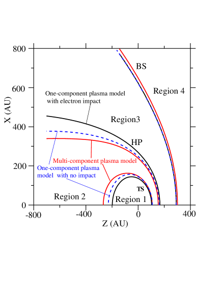
Figure 1: The termination shock, heliopause and bow shock shown for three models of the heliospheric interface: 1) new multi-component model, 2) Baranov & Malama model, 3) Baranov & Malama model with no electron impact.

The system of the equations for the velocity distribution function of H-atoms (Eq. (1)) and for mass, momentum and energy conservation for the total ionized component (Eqs. (2)) is not self-consistent, since it includes the velocity distribution function of pickup protons. At the present time there are many observational evidences (e.g. Gloeckler et al. 1993, Gloeckler 1996, Gloeckler & Geiss 1998) and theoretical estimates (e.g. Isenberg 1986), which clearly show that pickup ions constitute a separate and very hot population in the solar wind. Even though some energy transfer from the pickup ions to solar wind protons is now theoretically admitted in order to explain the observed heating of the outer solar wind (Smith et al. 2001; Isenberg et al. 2003, Richardson & Smith 2003, Chashei et al. 2003, Chalov et al. 2004b), it constitutes not more than 5% of the pickup ion energy. The observations show also that the velocity distribution function can be considered as isotropic (fast pitch-angle scattering) except some short periods in the inner heliosphere when the interplanetary magnetic field is almost radial.

So we assume here that the velocity distribution of pickup protons in the solar wind rest frame is isotropic, and it is determined through the velocity distribution function in the heliocentric coordinate system by the expression:

$$f_{pui}^{*}(\@vec{r},w)=\frac{1}{4\pi}\int\int f_{pui}(\@vec{r},\@vec{v})sin\theta d\theta d\phi.$$ (2)

Here $\@vec{v}=\@vec{u}+\@vec{w}$, $\@vec{v}$ and $\@vec{u}$ are the velocity of a pickup proton and bulk velocity of the plasma component in the heliocentric coordinate system, $\@vec{w}$ is the velocity of the pickup proton in the solar wind rest frame, and ($w$, $\theta$, $\phi$) are coordinates of $\@vec{w}$ in the spherical coordinate system. The equation for $f_{pui}^{*}(\@vec{r},w)$ can be written in the following general form taking into account velocity diffusion but ignoring spatial diffusion, which is unimportant at the energies under consideration:

$$\frac{\partial f_{pui}^{*}}{\partial t}+\@vec{u}\cdot\frac{\partial f_{pui}^{*}}{\partial\@vec{r}}=\frac{1}{w^{2}}\frac{\partial}{\partial w}\left(w^{2}D\frac{\partial f_{pui}^{*}}{\partial w}\right)+$$ (3)

$$+\frac{w}{3}\frac{\partial f_{pui}^{*}}{\partial w}div(\@vec{u})+S(\@vec{r},w),$$

where $D(\@vec{r},w)$ is the velocity diffusion coefficient. The source term $S(\@vec{r};w)$ can be written as

$$S(\@vec{r};w)=\frac{1}{4\pi}\int\int\nu_{ion}(\@vec{w})f_{H}(\@vec{r},\@vec{w}+\@vec{u})sin\theta d\theta d\phi$$ (4)

$$-\frac{1}{4\pi}\int\int f_{pui}^{*}(\@vec{r},w)\nu_{H}(\@vec{w})sin\theta d\theta d\phi.$$

In equation (5) $\nu_{ion}$ and $\nu_{H}$ are ionization rates:

$$\nu_{ion}=\sum_{i=pui,p}\int\int\int f_{i}^{*}(\@vec{r},w_{i})|\@vec{w}_{i}-\@vec{w}|\times$$

$$\sigma^{\rm HP}_{ex}(|\@vec{w}_{i}-\@vec{w}|)w_{i}^{2}dw_{i}sin\theta_{i}d\theta_{i}d\phi_{i}+\nu_{\rm ph}+\nu_{\rm impact},$$

$$\nu_{H}=\int f_{H}(\@vec{r},\@vec{v}_{H})|\@vec{w}+\@vec{u}-\@vec{v}_{H}|\sigma^{\rm HP}_{ex}(|\@vec{w}+\@vec{u}-\@vec{v}_{H}|)\,d\@vec{v}_{H}.$$

Although only stationary solutions of Eq. (4) will be sought here, we prefer to keep the first term in the equation to show its general mathematical structure. The effective thermal pressure of the pickup ion component is determined by

$$p_{pui}=\frac{4\pi}{3}\int m_{p}w^{2}f_{pui}^{*}(\@vec{r},w)w^{2}dw.$$ (5)

We solve the continuity equations for He⁺ in the interstellar medium and for alpha particles in the solar wind. Then proton number density can be calculated as $n_{p}=(\rho-m_{He}n_{He})/m_{p}-n_{pui}$. Here $n_{He}$ denotes the He⁺ number density in the interstellar medium, and He⁺⁺ the number density in the solar wind.

In addition to the system of equations (1), (2), (4) we solve the heat transfer equation for the electron component:

$$\frac{\partial\rho_{e}\varepsilon_{e}}{\partial t}+div([\rho_{e}\varepsilon_{e}]\@vec{u})=$$ (6)

$$-p_{e}div\@vec{u}+q_{3,e}+Q_{e,p}+Q_{e,pui}.$$

Here $\varepsilon_{e}=p_{e}/(\gamma-1)\rho_{e}$ is the specific internal energy of the electron component, $Q_{e,p}$ and $Q_{e,pui}$ are the energy exchange terms of electrons with protons and pickup ions, respectively.

To complete the formulation of the problem we need to specify: a) the diffusion coefficient $D(\@vec{r},w)$, b) exchange terms $Q_{e,p}$, $Q_{e,pui}$, c) the behavior of pickup protons and electrons at the termination shock. In principle, our model allows us to make any assumptions and verify any hypothesis regarding these parameters. Moreover, the diffusion coefficient $D(\@vec{r},w)$ depends on the level of solar wind turbulence, and equations describing the production (say, by pickups) and evolution of the turbulence need to be added to equations (1)-(7). This work is still in progress and will be described elsewhere.

In this paper we consider as simple a model as possible. We adopt $D=0$. While velocity diffusion is not taken into account in the paper, suprathermal tails in the velocity distributions of pickup protons are formed as will be shown below.

It is believed that the thickness of the termination shock ramp lies in the range from the electron inertial length up to the ion inertial length: $c/\omega_{\mathrm{e}}\leq L_{\mathrm{r}amp}\leq c/\omega_{\mathrm{p}}$, where $\omega_{\mathrm{e},p}=\left(4\pi n_{\mathrm{e},p}e^{2}/m_{\mathrm{e},p}\right)^{1/2}$ are the electron and proton plasma frequencies (see discussion in Chalov 2005). Since this thickness is less than the gyro-radius of a typical pickup proton in front of the termination shock at least by a factor of 10, the shock is considered here as a discontinuity. In this case the magnetic moment of a pickup ion after interaction with a perpendicular or quasi-perpendicular shock is the same as it was before the interaction (Toptygin 1980, Terasawa 1979). The only requirement is that the mean free path of the ions is larger than their gyro-radius (weak scattering). For perpendicular or near perpendicular parts of the termination shock conservation of the magnetic moment leads to the following jump condition at the shock (Fahr & Lay 2000):

$$f_{2,pui}^{*}(\@vec{r},w)=C^{-1/2}f_{1,pui}^{*}(\@vec{r},w/\sqrt{C})\,$$ (7)

where $C=\rho_{2}/\rho_{1}$ is the shock compression. Although the termination shock can be considered as perpendicular at their nose and tail parts only (Chalov & Fahr 1996, 2000; Chalov 2005), Nevertheless, we assume here for the sake of simplicity that Eq. (7) is valid everywhere at the shock. It should be emphasized that we are forced to adopt this condition in our axisymmetric model because taking into account real geometry of the large-scale magnetic field near the shock requires one to take into account 1) the three-dimensional structure of the interface, 2) reflection of pickup ions at the termination shock due to abrupt change in the magnetic field strength and direction. While the reflection is a very important process to inject ions into anomalous cosmic rays, we will consider this complication of our present model in future work. Note that the concept of magnetic moment conservation is only one of the possible scenarios of the behavior of pickup ions at the termination shock. Other possibilities will also be considered in the future.

We assume also that $Q_{e,pui}=0$ and $Q_{e,p}$ is such that

$$T_{e}=T_{p}=T_{He^{++}}$$

everywhere in the solar wind. Because of this assumption, there is no need to solve Es. (7). Nevertheless, we solve this equation in order to check numerical accuracy of our solution. Later, we plan to explore models with more realistic $D$ ,$Q_{e,pui}$ and $Q_{e,p}$ and different microscopic theories can be tested.

The boundary conditions for the charged component are determined by the solar wind parameters at the Earth’s orbit and by parameters in the undisturbed LIC. At the Earth’s orbit it is assumed that proton number density is n_p,E=n_e,E=7.72 cm^-3, bulk velocity is $u_{E}$=447.5 km/s and ratio of alpha particle to proton is 4.6 %. These values were obtained by averaging the OMNI 2 solar wind data over two last solar cycles. The velocity and temperature of the pristine interstellar medium were recently determined from the consolidation of all available experimental data (M$\mathrm{\ddot{o}}$bius et al. 2004, Witte 2004, Gloeckler 2004, Lallement 2004a,b). We adopt in this paper V_LIC= 26.4 km/s and T_LIC=6527 K.

For the local interstellar H atom, proton and helium ion number densities we assume n_H,LIC = 0.18 cm^-3, n_p,LIC=0.06 cm^-3 and n${}_{He^{+},LIC}$=0.009 cm^-3 , respectively (for argumentation, see, e.g., Izmodenov et al. 2003, 2004). The velocity distribution of interstellar atoms is assumed to be Maxwellian in the unperturbed LIC. For the plasma component at the outer boundary in the tail we used soft outflow boundary conditions. For the details of the computations in the tail direction see Izmodenov & Alexashov (2003), Alexashov et al. (2004b).

To solve the system of governing Euler equations for the plasma component, the second order finite volume Godunov type numerical method was used (Godunov et al. 1979; Hirsch 1988). To increase the resolution properties of the Godunov scheme, a piecewise linear distribution of the parameters inside each cell of the grid is introduced. To achieve the TVD property of the scheme the minmod slope limiter function is employed (Hirsch 1988). We used an adaptive grid as in Malama (1991) that fits the termination shock, the heliopause and the bow shock. The kinetic equation (1) was solved by the Monte-Carlo method with splitting of trajectories following Malama (1991). The Fokker-Planck type equation (4) for the pickup proton velocity distribution function is solved by calculating statistically relevant numbers of stochastic particle trajectories (Chalov et al., 1995). To get a self-consistent solution of the plasma Euler equations (2), kinetic equation (1) and Fokker-Planck type eq. (4) we used the method of global iterations suggested by Baranov et al. (1991).

Table 1: Description of introduced types of protons and populations of H atoms.

Type number	Proton type description
0	’cold proton type’ consisting of:
	original solar wind protons + protons
	created in region 1 from atoms of
	population 1.0 + protons created
	in region 2 from atoms of populations
	2.0, 3, 4
1	pickup protons created in region 1 from
	atoms of populations 1.1, 2.0, 3, 4
2	pickup protons created in region 1 from
	atoms of populations 1.2, 2.1-2.4
3	pickup protons created in region 2 from
	atoms of populations 1.0, 1.1
4	pickup protons created in region 2 from
	atoms of populations 1.2, 2.1-2.4
Population number	H atoms created in:
1.0	region 1 from protons of type 0
1.1	region 1 from pickup protons of type 1
1.2	region 1 from pickup protons of type 2
2.0	region 2 from protons of type 0
2.1	region 2 from pickup protons of type 1
2.2	region 2 from pickup protons of type 2
2.3	region 2 from pickup protons of type 3
2.4	region 2 from pickup protons of type 4
3	secondary interstellar atoms (as previously)
4	primary interstellar atoms (as previously)

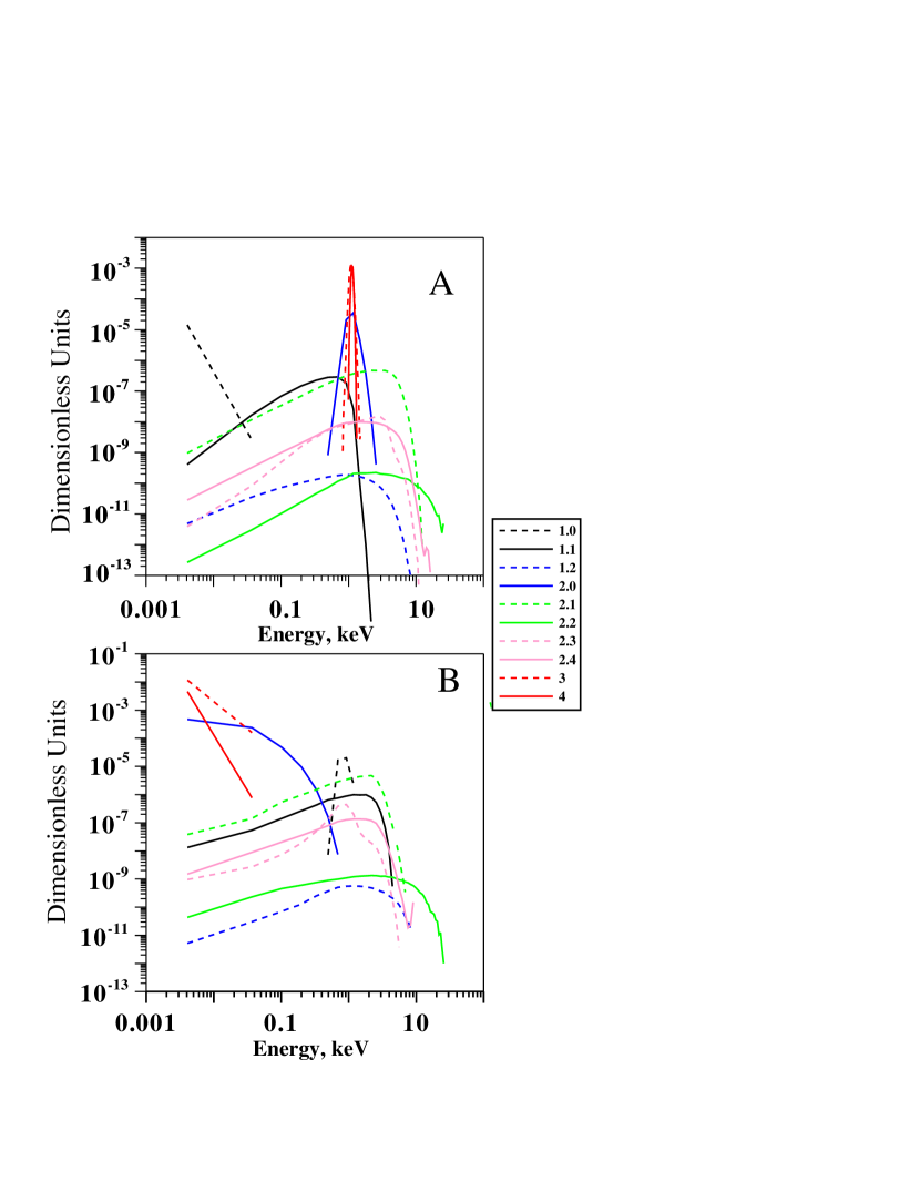
Figure 2: The source term S (Eq. (4)) from different populations of H atoms as a function of energy shown in the supersonic solar wind at 5 AU (A) and in the inner heliosheath (B).

3 Results of numerical modeling

Figures 1-6 present the main results obtained in the frame of our new multi-component model described in the previous section. The shapes and locations of the termination shock (TS), heliopause (HP) and bow shock (BS) are shown in Fig. 1. For the purposes of comparison the positions of the TS, HP, and BS are also shown in the case when pickup and solar wind protons are treated as a single fluid. Later we refer to this model as the Baranov-Malama (B&M) model. Two different cases obtained with the B&M model are shown. In the first case ionization by electron impact is taken into account, while this effect is omitted in the second case. The only (but essential) difference between the B&M model and our new model, considered in this paper, is that the latter model treats pickup protons as a separate kinetic component. As seen from Figure 1 the differences in the locations of the TS, HP, and BS predicted by the new and B&M models are not very large in the upwind direction. The TS is 5 AU further away from the Sun in the new model compared to B&M models. The HP is 12 AU closer. The effect is much more pronounced in the downwind direction where the TS shifts outward from the Sun by $\sim$70 AU in the new model. Therefore, the inner heliosheath region is thinner in the new model compared to the B&M model. This effect is partially connected with lower temperature of electrons and, therefore, with a smaller electron impact ionization rate in this region. Indeed, new pickup protons created by electron impact deposit additional energy and, therefore, pressure in the region of their origin, i.e. in the inner heliosheath. The additional pressure pushes the heliopause outward and the TS toward the Sun. Even though our multi-component model takes into account ionization by electron impact, this is not as efficient as in one-fluid models (like B&M) due to the lower electron temperature in the heliosheath. Excessively high electron temperatures which are predicted by the one-fluid models in the outer heliosphere are connected with the physically unjustified assumption of the immediate assimilation of pickup protons into the solar wind plasma.

However, the HP is closer to the Sun and the TS is further from the Sun in the new multi-component model even in the case when electron impact ionization is not taken into account. This is because the solar wind protons and pickup protons are treated in the new multi-component model as two separate components. Indeed, hot energetic atoms (ENAs), which are produced in the heliosheath by charge exchange of interstellar H atoms with both the solar wind protons and pickup protons heated by the TS, escape from the inner heliosheath easily due to their large mean free paths. These ENAs remove (thermal) energy from the plasma of the inner heliosheath and transfer the energy to other regions of the interface (e.g., into the outer heliosheath). In the case of the new model there are two parenting proton components for the ENAs - the original solar protons and pickup protons. In the B&M model these two components are mixed to one. As a result, the ENAs remove energy from the inner heliosheath more efficiently in the case of the multi-component model than the B&M model not. Similar effect was observed for multi-fluid models of H atoms in the heliospheric interface described in detail by Alexashov & Izmodenov (2005).

To gain a better insight into the results of the new model and its potential possibilities to predict and interpret observational data, we divide heliospheric protons (original solar and pickup protons) into five types, and H atoms into ten populations described in Table 1. The first index in the notation of an H-atom population is the number of the region, where the population was created, i.e. populations 1.0-1.2 are the H atoms created in the supersonic solar wind (region 1, see Fig.1), populations 2.0-2.4 are the H atoms created in the inner heliosheath (region 2), populations 3 and 4 are secondary and primary interstellar atoms. Definitions of the two last populations are the same as in the B&M model. The second index denotes the parent charged particles (protons), i.e. from 0 to 4.

Original solar wind protons are denoted as type 0. Protons of this type are cold compared to the normal pickup protons in the solar wind. The pickup protons, which have characteristics close to the original solar wind protons, are also added to type 0. These are pickup protons created in the supersonic solar wind (region 1) from H atoms of population 1.0 (this population forms a so-called neutral solar wind, e.g. Bleszynski et al. 1992) and pickup protons created in the inner heliosheath (region 2) from H atoms of populations 2.0, 3, and 4. The type 0 is formed in such a way that 1) its thermal pressure is much less than the dynamic pressure everywhere in the heliosphere and, therefore, unimportant; 2) we are not interested in details of the velocity distribution of this type of protons and assume that it is Maxwellian. The rest of the pickup protons is divided into four types: two types are those pickup protons that are created in region 1 (supersonic solar wind), and the others are pickup protons created in region 2 (inner heliosheath). In each region of birth we separate pickup protons into two additional types depending on their energy (more precisely, parent atoms). For instance, type 1 is the ordinary pickup proton population which is created in the supersonic solar wind from primary and secondary interstellar atoms and then convected in the inner heliosheath. Type 2 is also created in the supersonic solar wind but, in distinction to type 1, from energetic atoms. Among pickup protons created in the inner heliosheath type 4 is more energetic than type 3. Thus, two types of pickup protons (1 and 2) exist in the supersonic solar wind and four (1-4) in the inner heliosheath, from which types 2 and 4 are more energetic than 1 and 3. A more detailed description of the properties of pickup protons of different types will be given below (Figs. 3-4).

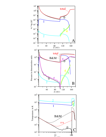
Figure 3: Number densities (A), thermal pressure (B) and temperature (C) of different types of protons. Curves are labelled with proton types.

One should keep in mind that at any place in the heliosphere real pickup protons constitute a full distribution and they are not divided into different types as we introduce here. However, and it is very important, the pickup protons have a rather broad energy spread, and, as we show below, particles with different places of birth and parent atoms prevail in a particular energy range according to our separation into the different types. The same is valid for H atoms. Thus one of the main advantages of our new model is the theoretical possibility to predict solar wind plasma properties in the outer parts of the heliosphere (including the inner heliosheath) through observations of pickup protons and hydrogen atoms in different energy ranges. Note that even without this rather complicated separation of particles into different types and populations but in the case when all pickup protons are treated as a distinct kinetic component (the simplest version of our model), the plasma flow pattern, positions and shapes of the TS, HP and BS are essentially the same.

As an useful illustration of the aforesaid, we present the calculated source term $S$ (see Eq. (4)) of pickup protons in the supersonic solar wind and in the heliosheath (Fig. 2). It is apparent that relative contributions of different H-atom populations into pickup protons are essentially different. In the supersonic solar wind (Fig. 2A) narrow peaks near 1 keV are created by populations 2.0, 3 and 4. These populations are seeds for the major type of pickup protons, which we denote as type 1. Pickup protons created from population 1.1 are also added to type 1 due to the lack of high energy tails in their distributions. Pickup protons created from H atoms of populations 1.2, 2.1-2.4 form type 2, which is more energetic compared to type 1 (see also argumentation above). A similar discussion can be applied to pickup protons created in the inner heliosheath.

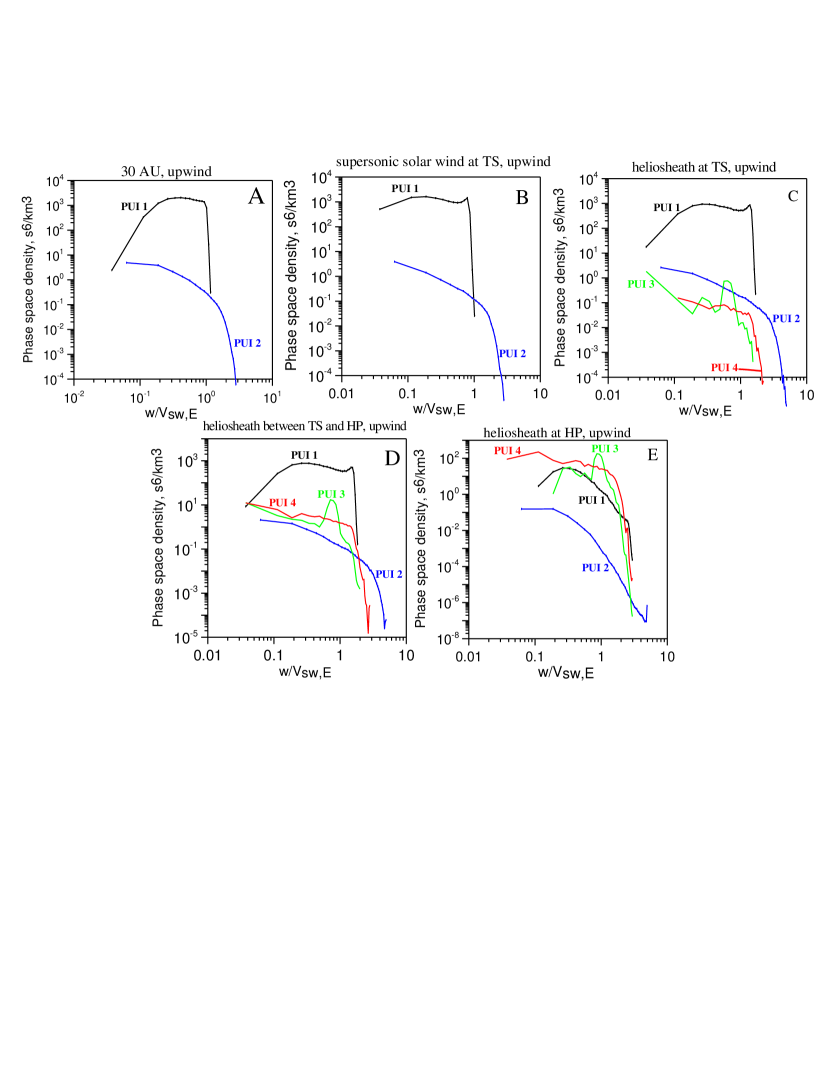
Figure 4: Phase space densities of different types of protons in the supersonic solar wind at 30 AU (A), upstream (B) and downstream (C) of the termination shock, inside the inner heliosheath (D) and at the heliopause (E). All curves are shown for the upwind direction.

It is important to underline here again that the main results of our model do not depend on the way we divide H atoms and pickup ions into populations and types. Such a division has two principal goals: 1) to have a clearer insight into the origin and nature of the pickup ions measured by SWICS/Ulysses and ACE (Gloeckler & Geiss 2004) and ENAs that will be measured in the near future (McComas et al. 2004), and 2) to obtain better statistics in our Monte Carlo method with splitting of trajectories (Malama 1991) when we calculate high energy tails in the distributions of pickup protons and H atoms that are several orders of magnitude lower than the bulk of particles.

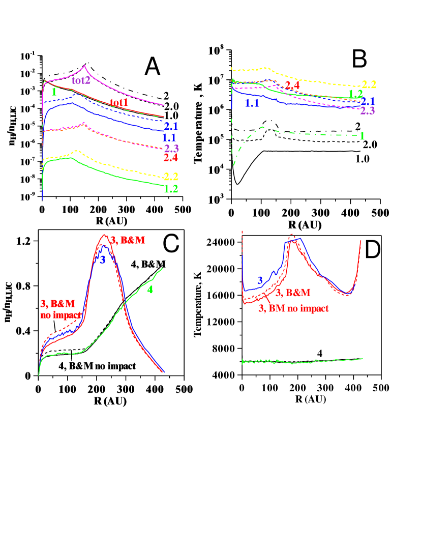
Figure 5: Number densities of H-atom populations 1.0-1.2, 2.0-2.4 (A) and populations 3,4 (C), and temperatures of these populations (B and D, respectively) as functions of heliocentric distance. Numeration of curves corresponds to numeration of the populations. Number densities and temperatures obtained with the Baranov and Malama (1993) model denoted as B&M and ”B&M no impact” are shown for comparison. The sum of the number densities of populations 1.0,1.1 and 1.2 are shown as curve ’tot1’. The sum of the number densities of populations 2.0-2.4 are shown as curve ’tot2’.

Number densities, pressures and temperatures for the introduced types of charged particles are shown in Fig. 3. It is seen (Fig. 3A) that the protons of type 0 (recall that these protons are mainly of solar origin) dominate by number density everywhere in the heliosphere, while type 1 of pickup protons makes up to 20 % of the total number density in the vicinity of the TS. Approaching the HP the number densities of types 1 and 2 decrease, since in accordance with our notation these types are created in the supersonic solar wind only. When the pickup protons are convected in the regions behind the TS, types 1 and 2 experience losses due to charge exchange with H atoms. New pickup protons created in the inner heliosheath as a result of this reaction have different properties than the original pickup protons (see below), and we assign them to types 3 and 4. The number densities of these types increase towards the HP.

Although the solar wind protons (type 0) are in excess in the number density, nevertheless pickup protons are generally much hotter (see Fig. 3C) and as a consequence the thermal pressure of type 1 dominates in the outer parts of the supersonic solar wind and in the inner heliosheath. Downstream of the TS this pressure is almost an order of magnitude larger than the pressure of type 0. As would be expected, the temperatures of types 2 and 4 are much larger than those of types 1 and 3, respectively. The temperature of the solar wind protons of type 0 decreases adiabatically up to 20 AU. Then the temperature becomes so low that the energy transferred to the solar wind by photoelectrons becomes non-negligible. This effect results in the formation of a plateau in the spatial distribution of the proton temperature in the region from 20 AU up to the TS. Figure 3C presents the proton temperature calculated with the B&M model for comparison. A highly unrealistic increase in the temperature is connected to the unrealistic assumption of immediate assimilation of pickup protons into the solar wind. Our new model is free of this assumption but it allows us to take into account some energy transfer between pickup and solar wind protons. The curve denoted as ”5%” in Fig. 3C shows the results of calculations, where we simply assume that 5 % of the thermal energy of pickup protons is transferred to the solar wind protons (to type 0). For pickup protons it is assumed that initial velocities (in the solar wind rest frame) of newly injected pickup protons are $\sim$2.5% smaller than the solar wind bulk velocity. The curve denoted as ”5%” is qualitatively very similar to the Voyager 2 observations which clearly show some increase in the proton temperature in the outer heliosphere. More prominent mechanisms of energy transfer between pickup and solar wind protons based on real microphysical background will be included in the model in the future.

Velocity distribution functions (in the solar wind rest frame) of the four types of pickup protons are shown in Fig. 4 for different heliocentric distances in the upwind direction. All distributions are presented as functions of the dimensionless speed $w/V_{\rm SW,E}$, where $V_{\rm SW,E}$ is the solar wind speed at the Earth’s orbit. In the supersonic solar wind (Fig. 4A,B) type 1 is dominant at energies below about 1 keV ($w<V_{\rm SW,E}$), while the more energetic type 2 is dominant for energies above 1 keV ($w>V_{\rm SW,E}$). As was shown for the first time by Chalov & Fahr (2003), this energetic type of pickup protons (secondary pickup protons) created in the supersonic solar wind from energetic hydrogen atoms can form the quite-time suprathermal tails observed by SWICS/Ulysses and ACE instruments (Gloeckler 1996, Gloeckler & Geiss 1998). Downstream of the TS up to the heliopause (Fig. 4C-E) the high-energy tails are more pronounced. The high-energy pickup ions form an energetic population of H atoms known as ENAs (e.g. Gruntman et al. 2001).

As we have discussed above and as is seen from Fig. 4, the pickup protons of type 1 prevail throughout the heliosphere except a region near the HP. In the supersonic solar wind the velocity distributions of these pickup protons are close to the distributions obtained by Vasyliunas & Siscoe (1976) who also ignored velocity diffusion. However, our distributions are different, since in our model 1) the solar wind speed varies with the distance from the Sun, 2) the spatial behavior of the ionization rate is more complicated, 3) thermal velocities of H atoms are taken into account, 4) the set of parent atoms is more varied (see Table 1). Note that we are forced to calculate the velocity distribution functions in the supersonic solar wind with a very high accuracy taking into account all above-mentioned effects self-consistently, since the proton temperature is several orders of magnitude lower than the temperature of the pickup protons (see Fig. 3C) and even small numerical errors in the temperature of the pickup protons can result in negative temperatures of the solar wind protons.

Figure 5 presents the number densities and temperatures of H-atom populations created inside (Fig.5A and 5B) and outside the heliopause (Fig.5C and 5D). The sum of the number densities of populations 1.0, 1.1, 1.2 is noted as ’tot1’, the sum of the number densities of populations 2.0-2.4 is noted as ’tot2’. For comparison we present the number densities of populations 1 and 2 of B&M model (denoted as curves 1 and 2). Curves ’tot1’ and ’1’ coincide, while curves ’tot2’ and ’2’ are noticeably different. The B&M model overestimates the total number density of populations 2.0-2.4. This is connected with the fact that ’temperatures’ (as measures of the thermal energy) of populations 2.1-2.4 are much above the temperature of population 2 in the B&M model. Inside 20 AU population 1.0 dominates in the number density, while outside the 20 AU population 2.0 becomes dominant. Figure 6 presents differential fluxes of different populations of H atoms at 1 AU. It is seen that different populations of H atoms dominate in different energy ranges. At the highest energies of above 10 keV, population 2.2 dominates. This population consists of atoms created in the inner heliosheath from hot pickup protons of type 2. Population 2.1 dominates in the energy range of 0.2-6 keV . This population consists of atoms created in the inner heliosheath from hot pickup protons of type 1. Since the both populations are created in the inner heliosheath the measurements of these energetic particles as planned by IBEX will provide robust information on the properties of the inner heliosheath and, particulary, on the behavior of pickup ions in this region. Note also that there is a significant difference in the ENA fluxes predicted in the frame of one- and multi- component models.

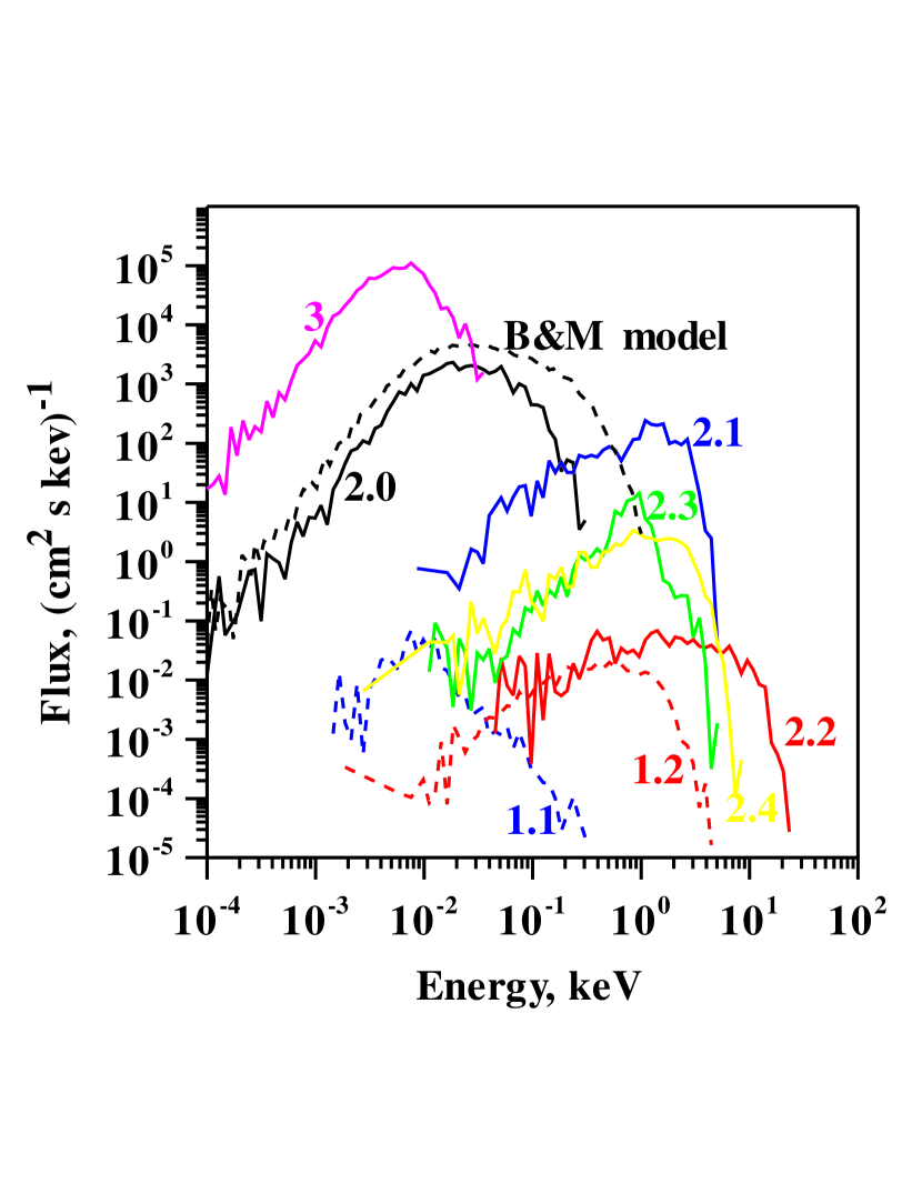
Figure 6: Fluxes of H atoms of populations 1.1,1.2, 2.0-2.4 and 3 at 1 AU in the upwind direction as functions of energy.

Returning to Figures 5C and 5D, the filtration factor, i.e. the amount of interstellar H atom penetrating through the interface, and the temperature of population 3 are noticeably different in the new multi-component model than the B&M model. This could lead to changes in interpretation of those observations, which require knowledge of the interstellar H atom parameters inside the heliosphere, say at the TS.

4 Conclusions

We have developed a new self-consistent kinetic-continuum model which includes the main advantage of our previous models, i.e. a rigorous kinetic description of the interstellar H-atom flow, and takes into account pickup protons as a separate kinetic component. The new model is very flexible and allows us to test different scenarios for the pickup component inside, outside and at the termination shock. The model allows to treat electrons as a separate component and to consider different scenarios for this component. We have created a new tool for the interpretation of pickup ions and ENAs as well as all diagnostics, which are connected with the interstellar H-atom component. The new model requires a more exact description of the physical processes involved than previous non self-consistent models. It is shown that the heliosheath becomes thinner and the termination shock is further from the Sun in the new model than the B&M model. The heliopause, however, is closer.

The main methodological advancements made in the reported model, which was not discussed in this paper, is that we successfully applied the Monte Carlo method with splitting of trajectories (Malama 1991) to non-Maxwellian velocity distribution functions of pickup protons. The splitting of trajectories allows us to improve the statistics of our method essentially and to calculate differential fluxes of ENAs at 1 AU with a high level of accuracy. We showed that ENAs created from different types of pickup protons dominate in different energy ranges that allows us to determine the nature of the heliosheath plasma flow.

Acknowledgement. We thank our referee, Hans J. Fahr, for valuable suggestions that improved this paper. The calculations were performed using the supercomputer of the Russian Academy of Sciences. This work was supported in part by INTAS Award 2001-0270, RFBR grants 04-02-16559, 04-01-00594, RFBR-CNRS (PICS) project 05-02-22000a and Program of Basic Researches of OEMMPU RAN. Work of V.I. was also supported by NASA grant NNG05GD69G, RFBR-GFEN grant 03-01-39004, and International Space Science Institute in Bern.

References

- Alexashov et al., (2000) Aleksashov D. B., Baranov V. B., Barsky E. V., Myasnikov A. V., 2000, Astron. Let. 26, 743
- Alexashov et al., (2004) Alexashov D. B., Chalov S. V., Myasnikov A. V., et al., 2004, &A 420, 729
- Alexashov et al. (2004b) Alexashov, D. B., Izmodenov, V. V., & Grzedzielski, S. 2004b, Adv. Space Res., 34, 109
- Alexashov and Izmodenov (2005) Alexashov D. B., Izmodenov V. V., 2005, A&A, accepted
- Baranov et al. (1991) Baranov V.B., Labedev, M.G., Malama, IU.G., 1991, ApJ 375, 347.
- Baranov & Malama (1993) Baranov V.B., Malama Y.G., 1993, J. Geophys. Res. 98, 15157
- Błeszynski et al. (1992) Błeszynski S., Grzedzielski S., Rucinski D., Jakimiec J., 1992, Planet. Space Sci. 40, 1525
- Bogdan et al., (1991) Bogdan T.J., Lee M.A., Schneider P., 1991, J. Geophys. Res. 96, 161
- Chalov (2005) Chalov S.V., 2005, Adv. Space Res. (in press)
- Chalov & Fahr (1996) Chalov S.V., Fahr H.J., 1996, Solar Phys., 168, 389
- Chalov & Fahr (2000) Chalov S.V., Fahr H.J., 2000, A&A, 360, 381
- Chalov & Fahr (2003) Chalov S.V., Fahr H.J., 2003, A&A 401, L1
- Chalov et al. (1997) Chalov S.V., Fahr H.J., Izmodenov V. V., 1997, A&A 320, 659
- (14) Chalov S.V., Fahr H.J., Izmodenov V. V., 2003, J. Geophys. Res. 108, 1266
- (15) Chalov S.V., Izmodenov V.V., Fahr H.J., 2004a, Adv. Space Res. 34, 99
- (16) Chalov S.V., Alexashov D.B., Fahr H.J., 2004b, A&A, 416, L31
- Chashei et al., (2003) Chashei I., Fahr H.J. Lay G., 2003, Ann. Geophys. 21, 1405.
- Fahr and Lay (2000) Fahr H. J., Lay G., 2000, A&A, 356, 327
- Fahr et al. (2000) Fahr H. J., Kausch T., Scherer H., 2000, A&A 357, 268
- Fichtner et al., (1996) Fichtner H., le Roux J.A., Mall U., Rucinski D., 1996, A&A 314, 650
- Fisk, (1976) Fisk L.A., 1976, J. Geophys. Res. 81, 4633
- Godunov (1979) Godunov, S.K. (Ed.), 1979, Resolution Numerique des Problems Multidimensionnels de la Dynamique des Gaz, Editions MIR, Moscow.
- Gloeckler (1996) Gloeckler G., 1996, Space Sci. Rev. 78, 335
- Gloeckler & Geiss (1998) Gloeckler, G., Geiss, J. 1998, Space Sci. Rev. 86, 127
- Gloeckler & Geiss (2004) Gloeckler G., Geiss J., 2004, Adv. Space Res. 34, 53
- Gloeckler et al. (1993) Gloeckler, G., Geiss, J., Balsiger, H., Fisk, L.A., Galvin, A.B., Ipavich, F.M., Ogilvie, K.W., von Steiger, R., Wilken, B. 1993, Science, 261, 70
- Gloeckler et al. (2004) Gloeckler, G., Mbius, E., Geiss, J., et al. 2004, Astron. Astrophys., 426, 845
- Gruntman et al. (2001) Gruntman M., Roelof E.C., Mitchell D.G., et al., 2001, J. Geophys. Res. 106, 15767
- Hirsch (1988) Hirsch, C., 1988, Numerical Computation of internal and external flows, Vol.2, John Willey and Sons, 691 pp.
- Isenberg (1986) Isenberg P.A., 1986, J. Geophys. Res. 91, 9965
- Isenberg, (1987) Isenberg P.A., 1987, J. Geophys. Res. 92, 1067
- Isenberg et al. (2003) Isenberg P.A., Smith C.W., Matthaeus W.H. 2003, ApJ, 592, 564
- Izmodenov et al., (2003) Izmodenov V.V., Malama Y.G., Gloeckler G., Geiss, J., 2003, ApJ Let. 954, L59
- Izmodenov, (2004) V. Izmodenov, 2004, p. 23, in ”The Sun and the Heliosphere as an Integrated System” Poletto & Suess (Eds), Kluwer.
- (35) Izmodenov V., Malama Y., Ruderman M. S., 2005a, A&A 429, 1069
- Izmodenov et al., (2004) Izmodenov, V.V., Malama, Y., Gloeckler, G., Geiss, J. 2004, A & A 414, L29).
- Izmodenov and Alexashov (2003) Izmodenov, V. V., & Alexashov, D. 2003, Astron. Let., 29, 58.
- (38) Izmodenov V.V., Alexashov D.B., Myasnikov A.V., 2005b, A&A 437, L35 L38.
- (39) Lallement, R., Raymond, J. C., Vallerga, J., et al., 2004a, Astron. Astrophys. 426, 875
- (40) Lallement, R., Raymond, J. C., Bertaux, J.-L., et al., 2004b, Astron. Astrophys. 426, 867.
- le Roux and Ptuskin, (1998) le Roux J.A., Ptuskin V.S., 1998, J. Geophys. Res. 103, 4799
- Malama (1991) Malama Yu.G., 1991, Astrophys. Space Sci. 176, 21
- McComas et al. (2004) McComas D., Allegrini F. Bochsler P., et al., 2004, AIP Conf. Proc. 719, 162.
- Moebius et al. (2004) Mbius, E., Bzowski, M., Chalov, S., et al., 2004, A & A 426, 897-907.
- Myasnikov et al., (2000) Myasnikov A. V., Alexashov D. B., Izmodenov V. V., Chalov S. V., 2000, J.Geophys. Res. 105, 5167
- Richardson & Smith (2003) Richardson J.D., Smith C.W. 2003, Geophys. Res. Lett., 30, 1206
- Smith et al. (2001) Smith C.W., Matthaeus W.H., Zank G.P., et al. 2001, J. Geophys. Res., 106, 8253
- Terasawa (1979) Terasawa T., 1979, Planet. Space Sci. 27, 193
- Toptygin (1980) Toptygin I.N., 1980, Space Sci. Rev. 26, 157
- Vasyliunas & Siscoe (1976) Vasyliunas V.M., Siscoe G.L., 1976, J. Geophys. Res. 81, 1247
- Wang and Richardson, (2001) Wang C., Richardson J.D., 2001, J. Geophys. Res. 106, 29401
- Witte (2004) Witte, M., 2004, Astron. Astrophys. 426, 835.
- Zank (1999) Zank G.P., 1999, Space Sci. Rev. 89, 413