Spontaneous Isotropy Breaking: A Mechanism for CMB Multipole Alignments

Abstract

We introduce a class of models in which statistical isotropy is broken spontaneously in the CMB by a non-linear response to long-wavelength fluctuations in a mediating field. These fluctuations appear as a gradient locally and pick out a single preferred direction. The non-linear response imprints this direction in a range of multipole moments. We consider two manifestations of isotropy breaking: additive contributions and multiplicative modulation of the intrinsic anisotropy. Since WMAP exhibits an alignment of power deficits, an additive contribution is less likely to produce the observed alignments than the usual isotropic fluctuations, a fact which we illustrate with an explicit cosmological model of long-wavelength quintessence fluctuations. This problem applies to other models involving foregrounds or background anisotropy that seek to restore power to the CMB. Additive models that account directly for the observed power exacerbate the low power of the intrinsic fluctuations. Multiplicative models can overcome these difficulties. We construct a proof of principle model that significantly improves the likelihood and generates stronger alignments than WMAP in 30-45% of realizations.

I Introduction

Data from the first year of WMAP has largely confirmed the standard cosmological model based on nearly scale-invariant statistically homogeneous and isotropic fluctuations Bennett et al. (2003a). Yet interestingly the large angle deficit in temperature fluctuations versus the standard model, first seen by COBE Smoot et al. (1992), was both confirmed and sharpened. This result is unlikely at between 0.7% and 10%, depending on the assumptions, the choice of statistic, and the analysis (Efstathiou, 2004; Slosar et al., 2004; Bielewicz et al., 2004; O’Dwyer et al., 2004). Cosmological explanations for a deficit of power involve breaking scale-invariance initially, dynamically, or topologically.

More recently, however, several other anomalies have been noted that point to a possible breaking of statistical isotropy on large angles. Statistically isotropy requires that all of the multipole moments of the CMB temperature field be uncorrelated at the two point level. Yet the WMAP data exhibit curious correlations or alignments in the temperature field. In particular, the octopole of the CMB is highly planar and aligned with the quadrupole (Tegmark et al., 2003; de Oliveira-Costa et al., 2004). Specifically the normalized angular momentum of the octopole is anomalously large at the 1/20 level and the angular momentum directions of the quadrupole and octopole are anomalously close at the 1/60 level. These and other alignments in the large-angle CMB have been further discussed and analyzed by Refs. (Copi et al., 2004; Schwarz et al., 2004; Land and Magueijo, 2005a, b; Bielewicz et al., 2004; Slosar and Seljak, 2004) and comprehensively studied in Ref. (Copi et al., 2005).

While the a posteriori nature of these statistics makes a strict interpretation of these probabilities difficult, the anomalies are clearly significant enough to merit serious attention. There are at least three classes of physical explanations: systematic, astrophysical, and cosmological. The WMAP instrument and time stream Hinshaw et al. (2003) have passed stringent tests that would make a systematic error of this magnitude and type difficult to conceive. An astrophysical explanation involving foreground contamination is certainly possible. However known foregrounds are accounted for very successfully (e.g. (Bennett et al., 2003b; Finkbeiner, 2004)) and the contamination would need to be of order the intrinsic CMB temperature anisotropy to account for the full effect. Still foreground and systematic contamination may weaken the significance of at least some of the statistical anomalies typically at the expense of others Slosar and Seljak (2004); Bielewicz et al. (2005); Copi et al. (2005).

The final possibility is that the anomalies have a cosmological explanation. Large-scale homogeneity and isotropy are clearly good assumptions for the universe as a whole. In this study, we examine the possibility that statistical isotropy is spontaneously broken in the fluctuations observed from a given spatial position and not in the fundamental theory. Correspondingly we will take the all-sky WMAP data Tegmark et al. (2003) at face value and ignore the possibility of foreground and systematic contamination. We begin in §II with the general mechanism and proceed in §III and §IV to describe two different implementations of the mechanism. We discuss these results in §V.

II Spontaneous Isotropy Breaking

We introduce a general mechanism for the breaking of isotropy in large angle fluctuations in §II.1. Under this mechanism statistical isotropy is preserved in the full theory but is spontaneously broken due to long-wavelength field fluctuations that appear as a gradient locally to the observer. A non-linear response to the field by CMB temperature fluctuations carries this preferred direction into a spectrum of multipoles. In §II.2 we discuss the statistical treatment of the induced correlations between multipole moments used in the following sections.

II.1 Non-linear Gradient Modulation

There are two ingredients in our mechanism for breaking the statistical isotropy. First, we require the presence of a field whose spatial fluctuations are dominated by long-wavelength contributions. Locally, around an observer, the structure in the field looks like a pure gradient. Given that a gradient must pick out a single direction, its presence provides the preferred axis for the breaking of isotropy. Because the long wavelength field is itself a random fluctuation, the underlying full theory retains statistical homogeneity and isotropy. Statistical isotropy is only apparently broken locally, and we refer to this as the spontaneous isotropy breaking.

The second ingredient is a non-linear response of the CMB temperature perturbations to this field. If the response were purely linear, then the field gradient would produce a dipole in the CMB. If the non-linearity were small, the higher order anisotropy would be increasingly suppressed with multipole number. A familiar example of this latter case is the Doppler effect due to the motion of the solar system through the CMB. The observed dipole is of course created by this motion. The effect on the quadrupole is a small correction to the true quadrupole proportional to $v^{2}$, while the corrections to the higher multipoles are entirely negligible Smoot et al. (1992). Here we seek to break isotropy in at least the quadrupole and octopole. Therefore the non-linearity must be substantial.

Let us now parameterize a class of model that possesses these ingredients. A pure gradient projected across the sky along some axis $\hat{\bf x}_{3}$ has the structure

$$G(\hat{\bf n})\propto(1+G_{1}\hat{\bf n}\cdot\hat{\bf x}_{3})=(1+G_{1}\cos\theta)\,,$$ (1)

where $\hat{\bf n}$ is the sky direction, $G_{1}$ is the relative amplitude of the gradient and $\theta$ is the polar angle from the preferred axis. A non-linear response to this gradient can be described as a general function of $G(\hat{\bf n})$, $F[G(\hat{\bf n})]$. This function can in turn be represented by its spherical harmonic coefficients with the pole aligned in the direction of the gradient axis

$$F[G(\hat{\bf n})]\equiv w(\hat{\bf n})=\sum_{\ell}w_{\ell}Y_{\ell 0}(\hat{\bf n})\,.$$ (2)

The azimuthal symmetry around the preferred axis of a gradient limits the coefficients to $m=0$.

In general, the CMB may exhibit a non-linear response in two different ways. It may produce an additive effect that is uncorrelated with the intrinsic anisotropy or it may produce a multiplicative modulation of this anisotropy. Furthermore, since the intrinsic anisotropy arises from a multitude of physical effects, it is possible that only one of them carries a non-linear response.

Thus let us model the temperature fluctuation field of the CMB as

$$T(\hat{\bf n})\equiv A(\hat{\bf n})+f[1+w(\hat{\bf n})]B(\hat{\bf n})\,,$$ (3)

where $A(\hat{\bf n})$ and $B(\hat{\bf n})$ are statistically isotropic Gaussian random fields. In the trivial case where $B(\hat{\bf n})=1$, the non-linear response is additive with an amplitude proportional to the parameter $f$. Alternately $A$ and $B$ may represent two different physical sources of the intrinsic anisotropy, e.g. the Sachs-Wolfe effect and the integrated Sachs-Wolfe effect. The non-linear modulation then produces a multiplicative breaking of isotropy in one of the effects.

II.2 Statistical Framework

It is convenient to describe the statistical properties of the model in terms of the multipole moments of the fields. The observed temperature field of Eq. (3) becomes

$$T(\hat{\bf n}) = \sum_{\ell m}t_{\ell m}Y_{\ell m}(\hat{\bf n})\,,$$ (4)

and similarly for the underlying isotropic fields

$$A(\hat{\bf n}) = \sum_{\ell m}a_{\ell m}Y_{\ell m}(\hat{\bf n})\,,$$

$$B(\hat{\bf n}) = \sum_{\ell m}b_{\ell m}Y_{\ell m}(\hat{\bf n})\,.$$ (5)

The assumption of statistical isotropy for the underlying fields $A$ and $B$ requires that their covariance matrices satisfy

$$\langle a_{\ell m}^{*}a_{\ell^{\prime}m^{\prime}}\rangle = \delta_{\ell\ell^{\prime}}\delta_{mm^{\prime}}C_{\ell}^{aa}\,,$$

$$\langle a_{\ell m}^{*}b_{\ell^{\prime}m^{\prime}}\rangle = \delta_{\ell\ell^{\prime}}\delta_{mm^{\prime}}C_{\ell}^{ab}\,,$$

$$\langle b_{\ell m}^{*}b_{\ell^{\prime}m^{\prime}}\rangle = \delta_{\ell\ell^{\prime}}\delta_{mm^{\prime}}C_{\ell}^{bb}\,.$$ (6)

However statistical isotropy is not preserved in the observed temperature field $T(\hat{\bf n})$.

Taking the multipole moments of Eq. (3), the product $w(\hat{\bf n})B(\hat{\bf n})$ becomes a convolution

$$t_{\ell m}=a_{\ell m}+fb_{\ell m}+f\sum_{\ell_{1}\ell_{2}}R_{\ell m}^{\ell_{1}\ell_{2}}b_{\ell_{2}m}$$ (7)

with a coupling matrix written in terms of Wigner 3j symbols

$$R_{\ell m}^{\ell_{1}\ell_{2}} \equiv (-1)^{m}\sqrt{(2\ell+1)(2\ell_{1}+1)(2\ell_{2}+1)\over 4\pi}$$ (12)

$$\times\left(\begin{array}[]{ccc}\!\ell_{1}\!&\ell_{2}\!&\ell\!\\ \!0\!&0\!&0\!\end{array}\right)\left(\begin{array}[]{ccc}\!\ell_{1}\!&\ell_{2}\!&\ell\!\\ \!0\!&m\!&-m\!\end{array}\right)w_{\ell_{1}}\,.$$

The ensemble average of the multipole moments becomes

$$\langle t_{\ell m}^{*}t_{\ell^{\prime}m}\rangle = \delta_{\ell\ell^{\prime}}[C_{\ell}^{aa}+2fC_{\ell}^{ab}+f^{2}C_{\ell}^{bb}]$$ (13)

$$+f\sum_{\ell_{1}}\left[R_{\ell^{\prime}m}^{\ell_{1}\ell}(C_{\ell}^{ab}+fC_{\ell}^{bb})+(\ell\leftrightarrow\ell^{\prime})\right]$$

$$+f^{2}\sum_{\ell_{1}\ell_{1}^{\prime}\ell_{2}}R_{\ell m}^{\ell_{1}\ell_{2}}R_{\ell^{\prime}m}^{\ell_{1}^{\prime}\ell_{2}}C_{\ell_{2}}^{bb}\,.$$

Here the ensemble average is over realizations of the fields $A$ and $B$ with a fixed field $w$. The field $T({\bf n})$ exhibits broken statistical isotropy with different variances in $m$ modes of a given $\ell$ and a covariance between different $\ell$ modes.

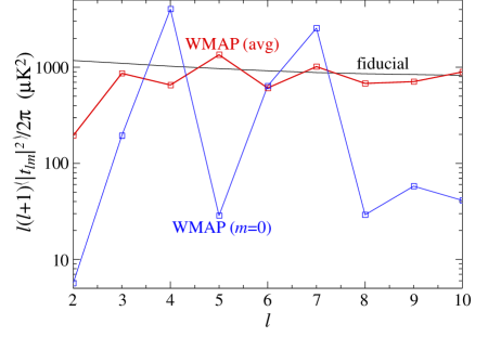
Figure 1: The fiducial cosmological model and the WMAP power in $\ell$ averaged over $m$ (“avg”) and from azimuthally symmetric (“$m=0$”) components in the dipole frame. In addition to an overall deficit of power in the quadrupole, the WMAP quadrupole and octopole exhibit a further reduction of power along the dipole direction. The fiducial cosmological model is defined by $\Omega_{m}=0.27$, $h=0.72$, $\Omega_{b}h^{2}=0.024$, $\delta_{\zeta}=5.07\times 10^{-5}$ and $\tau=0.17$.

For the simplest case of an additive effect $B(\hat{\bf n})=1$ and is not a stochastic field. We can however consider its effective power spectrum to be $C_{\ell}^{bb}=4\pi\delta_{\ell 0}$. The ensemble average of Eq. (13) reduces to

$$\langle t_{\ell m}^{*}t_{\ell^{\prime}m}\rangle = \delta_{\ell\ell^{\prime}}C_{\ell}^{aa}+f^{2}w_{\ell}w_{\ell^{\prime}}\delta_{m0}\,,$$ (14)

where $fw_{\ell}$ is a deterministic contribution or mean to the Gaussian distribution of $t_{\ell 0}$. A multiplicative model manifests more complex phenomenology. Here each $w_{\ell}$ correlates the observed multipoles across a range $\Delta\ell=\ell$. With a spectrum of $w_{\ell}$ the maximum range of the correlation is determined by the highest non-negligible mode in the spectrum. We will explore the additive and multiplicative versions in §III and §IV respectively.

A hallmark of this mechanism is that the modulation is azimuthally symmetric and hence couples harmonics with the same $m$ in the preferred frame. Note however that in a general coordinate system, for example galactic coordinates, different $m$ values will also be correlated.

Specifying the change in the coordinate system with Euler angles by rotating around the z-axis by $\phi\in[0,2\pi]$, then around the new y-axis by angle $\theta\in[0,\pi]$ and finally around the new z-axis by angle $\gamma\in[0,2\pi]$, the harmonic coefficients transform as (see for example Varshalovich et al. (1988))

$$\tilde{t}_{\ell\tilde{m}}=\sum_{m}t_{\ell m}D_{m\tilde{m}}^{\ell}(-\gamma,-\theta,-\phi)\,,$$ (15)

where the Wigner rotation matrix is given by

$$D_{m\tilde{m}}^{\ell}(\gamma,\theta,\phi)={\rm e}^{-i\tilde{m}\gamma}d_{m\tilde{m}}(\theta){\rm e}^{-im\phi}$$ (16)

and

$$d_{m{\tilde{m}}}(\theta)=$$

$$\sum_{k={\rm max}\{0,m+{\tilde{m}}\}}^{{\rm min}\{\ell+m,\ell+{\tilde{m}}\}}\left(\cos{\theta\over 2}\right)^{2k-m-{\tilde{m}}}\left(\sin{\theta\over 2}\right)^{2\ell+m+{\tilde{m}}-2k}$$

$$\times(-1)^{k+\ell+m}{\sqrt{(\ell+m)!(\ell-m)!(\ell+{\tilde{m}})!(\ell-{\tilde{m}})!}\over k!(\ell+m-k)!(\ell+{\tilde{m}}-k)!(k-m-{\tilde{m}})!}$$

is a real function. Thus the ensemble average becomes

$$\langle\tilde{t}_{\ell\tilde{m}}^{*}\tilde{t}_{\ell^{\prime}\tilde{m}^{\prime}}\rangle=\sum_{m}\langle t_{\ell m}^{*}t_{\ell^{\prime}m}\rangle D_{m\tilde{m}}^{\ell*}D_{m\tilde{m}^{\prime}}^{\ell}\,,$$ (17)

and exhibits completely broken isotropy.

Table 1: WMAP data vs. fiducial model in the dipole vs maximum angular momentum direction (see §IV.2). $N_{\ell}/C_{\ell}^{\rm fid}$ shows the relative contribution of noise assumed.

$\ell$	$m$	$C_{\ell}^{\rm fid}(\mu$K${}^{2})$	$N_{\ell}/C_{\ell}^{\rm fid}$	$|t_{\ell m}|^{2}/C_{\ell}^{\rm fid}$
				dipole	$\hat{L}^{2}_{\rm max}$
2	0	1233	0.005	0.005	0.005
	1			0.013	0.003
	2			0.396	0.406
3	0	577	0.007	0.179	0.315
	1			0.079	0.003
	2			0.426	0.029
	3			2.155	2.560
4	0	322	0.009	3.929	1.641
	1			0.156	0.939
	2			0.052	0.508
	3			0.271	0.401
	4			0.406	0.180
5	0	202	0.011	0.035	0.014
	1			0.376	0.811
	2			0.035	1.254
	3			6.827	2.777
	4			0.077	2.769
	5			0.364	0.078

In Tab. 1 and Fig. 1, we compare the power in the observed multipole moments of WMAP in the dipole frame to $C_{\ell}^{\rm fid}$, the power spectrum of a fiducial isotropic $\Lambda$CDM model. This model, which we use throughout the paper, has $\Omega_{m}=1-\Omega_{Q}=0.27$, $h=0.72$, $\Omega_{b}h^{2}=0.024$, $\delta_{\zeta}=5.07\times 10^{-5}$ and $\tau=0.17$. The WMAP data is taken to be the cleaned full-sky map of Tegmark et al. (hereafter TOH; Tegmark et al. (2003)). Note that the $m=0$ components of the quadrupole and octopole are low both with respect to the average over $m$ in the WMAP data and compared with the fiducial model. Thus the power deficit in the quadrupole and octopole are aligned. With broken statistical isotropy it is in principle possible to explain these and other anomalies in the power distribution of the data.

By employing the TOH cleaned map we are ignoring residual foregrounds and systematics. While these may or may not weaken the significance of alignments in the data (Bennett et al., 2003b; Eriksen et al., 2004a; Slosar and Seljak, 2004; Bielewicz et al., 2004; Copi et al., 2005), they do not affect the ability of a cosmological model to produce them. The latter is the main topic we address in this work.

III Additive Isotropy Breaking

To illustrate the idea of spontaneous isotropy breaking we first take the simple case of an additive contribution to the anisotropy. Spontaneous isotropy breaking requires a non-linear response in the observed CMB temperature to an underlying gradient field. We begin with a motivating example of a known systematic effect, the non-linear response of a detector, in §III.1. This non-linear response modulates the CMB dipole into higher order anisotropy aligned with the dipole. We then apply this idea to a cosmological example involving dark energy density fluctuations in §III.2.

The statistical anisotropy caused by additive isotropy breaking generally produces alignments of excess power. While alignments of power deficits, like those seen in the quadrupole and octopole of the WMAP data, are possible we show in §III.3 that they are statistically less likely than a chance alignment in a statistically isotropic field. This conclusion holds true for any mechanism which seeks to restore power and hence statistical isotropy in the quadrupole and octopole by removing a contaminant that is uncorrelated with the intrinsic anisotropy.

III.1 Instrumental Example

A concrete but non-cosmological means of additive isotropy breaking is provided by the non-linearity of a detector responding to temperature fluctuations. Suppose that the detector responds to a true temperature signal of $G(\hat{\bf n})$ as

$$T_{\rm det}(\hat{\bf n}) = fF[G(\hat{\bf n})]=f\sum_{i}\alpha_{i}\left[{G(\hat{\bf n})\over f}\right]^{i}\,,$$ (18)

where $\alpha_{1}=1$. Here $f$ is an arbitrary normalization scale for the non-linearity of the response. If $\alpha_{i>1}\neq 0$ then $T_{\rm det}\neq G$ and the observed temperature is a non-linear modulation of the true temperature.

The dominant temperature signal in a differencing experiment is the dipole arising from our peculiar motion, $G(\hat{\bf n})=T_{\rm dip}\cos\theta$ in the dipole frame, with $T_{\rm dip}=3.35$mK. The non-linear response has the general form of Eqn. (3). Taking $f=T_{\rm dip}$,

$${T_{\rm det}(\hat{\bf n})\over T_{\rm dip}} = \alpha_{1}P_{1}(\cos\theta)+\alpha_{2}\left[{2\over 3}P_{2}(\cos\theta)+1\right]$$

$$+\alpha_{3}\left[{2\over 5}P_{3}(\cos\theta)+{3\over 5}P_{1}(\cos\theta)\right]+\ldots\,,$$

where $P_{\ell}=\sqrt{4\pi/(2\ell+1)}Y_{\ell 0}$ are the Legendre polynomials, and therefore

$$w_{2} = {4\over 3}\sqrt{\pi\over 5}\alpha_{2}+\ldots\,,$$

$$w_{3} = {4\over 5}\sqrt{\pi\over 7}\alpha_{3}+\ldots\,,$$ (20)

where $\ldots$ represent contributions from $i>3$. With $\alpha_{2}=\alpha_{3}\sim 10^{-2}$, the $10^{-3}$ dipole anisotropy is modulated into a $10^{-5}$ quadrupole and octopole anisotropy with $m=0$ in the dipole frame.

Given the observed multipole moments $t_{\ell m}$, the intrinsic anisotropy becomes

$$a_{\ell m}=t_{\ell m}-fw_{\ell}\delta_{m0}\,.$$ (21)

For multipole moments that are observed to be anomalously low, as is the case for the quadrupole and octopole moments of WMAP in the dipole direction (see Tab. 1), $t_{\ell m}\rightarrow 0$ and $|a_{\ell 0}|^{2}\rightarrow f^{2}w_{\ell}^{2}\delta_{m0}$. Thus the removal of the additive contribution restores power to the intrinsic sky and can bring it closer to a statistically isotropic distribution. Note that this restoration involves a chance cancellation between a Gaussian random realization of $a_{\ell m}$ and a fixed additive contribution $fw_{\ell}$. This will be important in addressing the probability of such an occurrence in §III.3.

Detector non-linearity is unlikely to be the actual source of the observed alignments. In this model, the nonlinearity of the response would be at the percent level for the $3.35$mK dipole. If this model were extrapolated to brighter sources, it would imply that $\sim 1$K sources completely saturate the response which is demonstrably not true for the WMAP instrument. Nonetheless, the non-linear detector response model provides a concrete and conceptually simple illustration of the isotropy breaking mechanism. It has the added benefit that it naturally picks out the dipole direction as the preferred axis along which the temperature is modulated as seen in the WMAP data.

III.2 Dark Energy Example

Cosmological examples of isotropy breaking follow a similar form but are more complicated to calculate. Here one must combine the dynamics of how the modulated field produces temperature fluctuations in physical space along with the projection along the line of sight onto angular space. The benefit of a cosmological model is that the spectrum $w_{\ell}$ of the additive contributions have a well defined shape and hence the model in principle has predictive power, e.g. an additive correction at relatively high multipoles predicts a specific change to the low order multipoles and vice versa.

As a concrete example, let us consider the Integrated Sachs-Wolfe (ISW) effect induced by spatial perturbations in the dark energy density from a quintessence field $Q$. If the perturbations to the field $Q$ are dominated by superhorizon scale fluctuations then within our horizon the field will look linear

$$Q_{i}=B_{0}+B_{1}x_{3}+\ldots\,,$$ (22)

where $B_{i}$ are constants, so that the local gradient picks out a preferred axis ${\bf x}_{3}$. The non-linear modulation is provided by the scalar field potential. Taking it to be of the form

$$V(Q)=V_{0}[1+f\cos(Q/M_{0})]\,,$$ (23)

the field gradient manifests itself as

$$V(Q_{i})=V_{0}[1+f\cos(k_{0}x_{3}+\delta)]\,,$$ (24)

where $k_{0}\equiv B_{1}/M_{0}$ and $\delta\equiv B_{0}/M_{0}$. This initial potential energy fluctuation is then transferred onto the CMB through the ISW effect and the dynamics of the field.

As the actual field gradients are from superhorizon wavelengths, the field will remain frozen provided its mass $m$ is small compared to the Hubble parameter $H$:

$${|m^{2}|\over H^{2}}=\left|{\partial^{2}V\over\partial Q^{2}}\right|{1\over H^{2}} \leq 3\left|{\partial^{2}V\over\partial Q^{2}}\right|{M_{\rm pl}^{2}\over V}\leq 3f\left({M_{\rm pl}\over M_{0}}\right)^{2}\,,$$

where $M_{\rm pl}=(8\pi G)^{-1/2}$ is the reduced Planck mass. Thus, if

$${M_{0}\over M_{\rm pl}}\gg f^{1/2}\,,$$ (25)

the field will not roll and the density field then carries potential energy fluctuations that are frozen. Its Fourier components are

$${\delta\rho_{Q}\over\rho_{Q}}({\bf k}) = {f\over 2}e^{i\delta}(2\pi)^{3}\delta({\bf k}-k_{0}\hat{\bf x}_{3})$$ (26)

$$+{f\over 2}e^{-i\delta}(2\pi)^{3}\delta({\bf k}+k_{0}\hat{\bf x}_{3})\,.$$

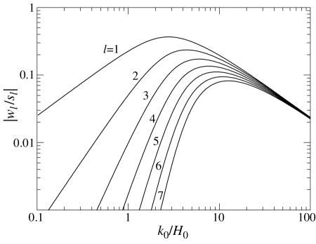
Figure 2: Dark energy based additive contributions $w_{\ell}$. Shown are the first few multipoles of $|w_{\ell}/s_{\ell}|$ as a function of $k_{0}/H_{0}$. Long wavelength perturbations exhibit a spectrum in $w_{\ell}$ that is steeply falling in $\ell$ and is modulated by parity considerations from $s_{\ell}$.

For the moment, we consider the case where only the dark energy is initially perturbed. The comoving curvature perturbation, $\zeta$, will evolve if there is a perturbation to the total pressure, $p_{T}$. As only the dark energy is perturbed, initially the Universe is effectively homogeneous, $\zeta_{i}=0$, and $\zeta$ only begins to grow during dark energy domination when the only non-negligible components to the total energy density $\rho_{T}$ are the dark energy density and the pressureless matter, $\rho_{m}$. The dark energy is assumed to be sufficiently light that it is approximately frozen and so $\rho_{Q}\approx-p_{Q}=$ const. The evolution of the comoving curvature perturbation, in a flat Universe, is given by (see for example the Appendix of Gordon and Hu (2004))

$$\zeta = \zeta_{i}-\int_{0}^{a}{da^{\prime}\over a^{\prime}}{\delta p_{T}\over{\rho_{T}+p_{T}}}$$ (27)

$$\approx \int_{0}^{a}{da^{\prime}\over a^{\prime}}{\delta\rho_{Q}\over\rho_{m}}\,.$$

Denoting the relative energy densities of dark energy and matter today as $\Omega_{Q}\equiv\rho_{Q}/\rho_{T}|_{a=1}$ and $\Omega_{m}\equiv\rho_{m}/\rho_{T}|_{a=1}$, the usual redshifting of pressureless matter can be written as

$$\rho_{m}={\rho_{Q}\over a^{3}}{\Omega_{m}\over\Omega_{Q}}\,.$$

Substituting this into Eq. (27) gives

$$\zeta={a^{3}\over 3}{\delta\rho_{Q}\over\rho_{Q}}{\Omega_{Q}\over\Omega_{m}}\,.$$ (28)

The Newtonian gravitational potential can be expressed in terms of $\zeta$ as (see for example Hu and Eisenstein (1999); Gordon and Hu (2004))

$$-\Psi({\bf k},a) = \zeta-{H\over a}\int_{0}^{a}{da^{\prime}\over H}\left(\zeta-{\delta p_{T}\over\rho_{T}+p_{T}}\right)$$ (29)

$$\approx \zeta-{H\over a}\int_{0}^{a}{da^{\prime}\over H}\left(\zeta+{\delta\rho_{Q}\over\rho_{m}}\right)\,.$$

Substituting Eqs. (27) and (26) into this gives

$$\Psi({\bf k},a)\approx\psi(2\pi)^{3}\delta({\bf k}-k_{0}\hat{\bf x}_{3})+\psi^{*}(2\pi)^{3}\delta({\bf k}+k_{0}\hat{\bf x}_{3})\,,$$ (30)

where

$$\psi=-{1\over 3}{\Omega_{Q}\over\Omega_{m}}{f\over 2}e^{i\delta}\left(a^{3}-4{H(a)\over a}\int{da^{\prime}\over H(a^{\prime})}{a^{\prime}}^{3}\right)\,.$$ (31)

When there are only dark energy perturbations, the temperature fluctuations in the direction $\hat{\bf n}$ due to the potential $\Psi$ are given by the ISW effect. Relating these contributions to the form of an additive isotropy breaking term in Eq. (3) gives

$${\Delta T(\hat{\bf n})\over T}=fw(\hat{\bf n})=\int 2\Psi^{\prime}({\bf x}=D\hat{\bf n},a)d\ln a\,,$$ (32)

where $D$ is the comoving distance along the line of sight and primes are derivatives with respect to $\ln a$. The multipole moments are given by

$$fw_{\ell}\equiv\int d\hat{\bf n}Y_{\ell m}^{*}({\hat{\bf n}}){\Delta T\over T}(\hat{\bf n})\,.$$ (33)

With the Rayleigh expansion of a plane wave

$$\exp(i{\bf k}\cdot{\bf x})=\sum_{\ell m}4\pi i^{\ell}j_{\ell}(kD)Y_{\ell m}^{*}({\hat{\bf k}})Y_{\ell m}({\hat{\bf n}})\,,$$ (34)

they can be written as

$$fw_{\ell}=\int d\ln a\int{d^{3}k\over(2\pi)^{3}}4\pi i^{\ell}j_{\ell}(kD)Y_{\ell m}^{*}({\hat{\bf k}})2\Psi^{\prime}({\bf k},a)\,.$$ (35)

Taking the form of the Newtonian gravitational potential above, we get

$$w_{\ell} = -{\Omega_{Q}\over{\Omega_{m}}}s_{\ell}\sqrt{4\pi(2\ell+1)}\int d\ln aj_{\ell}(k_{0}D)I(a)a^{3}\,,$$

$$s_{\ell} \equiv \cos\delta(-1)^{\ell/2}\delta_{\ell}^{\rm e}+\sin\delta(-1)^{(\ell+1)/2}\delta_{\ell}^{\rm o}\,,$$ (36)

where $\delta_{\ell}^{\rm e}=1$ if $\ell$ is even and 0 if $\ell$ is odd, and vice versa for $\delta_{\ell}^{\rm o}$. Here we have defined

$$I(a)\equiv-{8\over 3a^{3}}{d\over d\ln a}\left[{H(a)\over a}\right]\int{da^{\prime}\over H(a^{\prime})}{a^{\prime}}^{3}-{2\over 3}\,.$$ (37)

Given that the CMB response to a dark energy density perturbation is still linear, restoring adiabatic fluctuations is a simple matter of adding in the fiducial model contributions as an uncorrelated contribution to the temperature field.

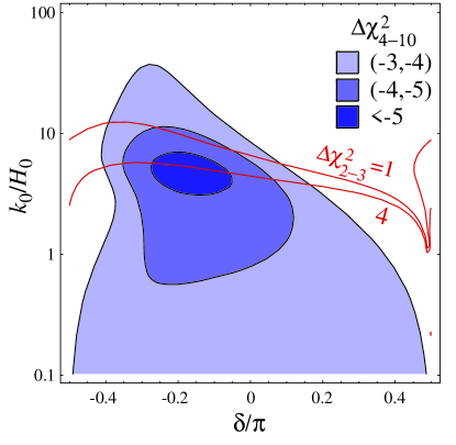
Figure 3: $\Delta\chi^{2}$ relative to the fiducial model for the additive model parameter space of phase and wavelength $(\delta,k_{0}/H_{0})$ with $f$ chosen to minimize the $\Delta\chi^{2}$. For the multipoles $\ell=4-10$, the maximum improvement is $\Delta\chi^{2}_{4-10}=-5.4$ (shaded contours). These models restore power to the quadrupole and octopole and thus $\ell=2,3$ add a disfavored positive contribution through $\Delta\chi^{2}_{2-3}$ (curves).

In Fig. 2, we show the amplitude of the first few multipoles of $w_{\ell}/s_{\ell}$ as a function of $k_{0}/H_{0}$ in the fiducial cosmological model. There are two general features in $w_{\ell}$ that go beyond the specifics of this model. First, a spatial modulation projects onto an angular modulation with a weight given by the spherical Bessel function $j_{\ell}$. For a superhorizon fluctuation

$$k_{0}D={k_{0}\over H_{0}}H_{0}D\sim{k_{0}\over H_{0}}\ll 1\,,$$ (38)

and so $j_{\ell}\propto(k_{0}/H_{0})^{\ell}$. Thus a superhorizon scale modulation typically predicts a sharply falling spectrum in $\ell$ for the additive contribution. The modulation scale $k_{0}$ should not be confused with the field gradient scale which is by assumption always superhorizon.

The symmetry factor $s_{\ell}$ provides an interesting modulation of this result, and this is the second general feature of the model. The phase of the plane wave $\delta$ determines its symmetry under a parity transformation $\hat{\bf n}\rightarrow-\hat{\bf n}$ or $\hat{\bf x_{3}}\rightarrow-\hat{\bf x_{3}}$. Because spherical harmonics have definite parity $(-1)^{\ell}$, the plane wave modulation affects even and odd multipole moments differently. In particular choosing a phase $\delta\rightarrow 0$, eliminates the contributions from all odd multipoles.

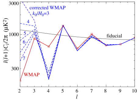
Figure 4: Restoration of power in the dark energy additive model. Taking a phase of $\delta=-0.173\pi$ that intersects the minimum $\Delta\chi_{4-10}^{2}$ from Fig. 3, models with wavelengths $k_{0}/H_{0}$ around the minimum restore power to the quadrupole and octopole (dashed line vs points) and bring them closer to the fiducial model (curve).

III.3 Power Excess and Restoration

Given the dark energy based model of the previous section, we can test the WMAP data for additive contributions that break statistical isotropy. We set the preferred axis for isotropy breaking to be in the direction of the dipole based on the observed pattern of low multipole alignments (e.g. de Oliveira-Costa et al. (2004); Schwarz et al. (2004); Land and Magueijo (2005a)). In the dipole frame, the observed power in $t_{\ell m}$ is given as a fraction of the power in the fiducial model of Fig. 1 in Tab. 1. The uneven distribution of power across $m$ for the quadrupole and octopole quantifies the alignment problem.

To determine whether the WMAP data favor an additive breaking of statistical isotropy, we maximize the likelihood with respect to model parameters. Since the additive contribution is deterministic and the underlying temperature field is assumed to be drawn from the fiducial model this amounts to minimizing the $\chi^{2}$

$$\chi^{2}=\sum_{\ell_{\rm min}}^{\ell_{\rm max}}(C_{\ell}+N_{\ell})^{-1}(t_{\ell m}^{*}-fw_{\ell}\delta_{m0})(t_{\ell m}-fw_{\ell}\delta_{m0})\,.$$ (39)

Here we have included a crude estimate of the noise in the WMAP data from their quoted power spectrum errors in the absence of sample variance. These are listed in Tab. 1. Note that our results here are insensitive to the specific representation of the noise as it is much smaller than the rms signal of the fiducial model.

The benefit of having a cosmological model for the additive contributions is that the functional form of the contributions is determined through $w_{\ell}$. Evidence for an alignment of excess power in one range of multipoles predicts the correction that must be applied to another. We therefore minimize the $\chi^{2}$ for $4\leq\ell\leq 10$ with respect to the parameters $(f,k_{0}/H_{0},\delta)$ and then examine what it implies for the quadrupole and octopole. The best-fit solution is $k_{0}/H_{0}=4.8,\delta=-0.173\pi,f=1.16\cdot 10^{-4}$ and has improvement of $\Delta\chi^{2}=-5.4$ relative to the fiducial model with no additive contribution. In fact, there is a wide range of models with a similar level of improvement ($\Delta\chi^{2}\sim-5$) since the two parameters $k_{0}/H_{0}$ and $\delta$ affect the $\ell$ dependence of the contributions similarly. We show in Fig. 3 the $\Delta\chi^{2}$ contours for $\ell=4-10$ in the ($k_{0}/H_{0}$, $\delta$) space for the best-fit amplitude $f$. About two thirds of the improvement in $\chi^{2}$ comes from $\ell=4$ which has a $\sim 2\sigma$ excess in power compared with the fiducial model (see Fig. 1 and Tab. 1).

Given this range of models that improve the $\Delta\chi^{2}$ for $\ell=4-10$, it is interesting to see what they imply for the quadrupole and octopole. In Fig. 4, we show the intrinsic WMAP power spectrum (i.e. one with the additive contribution removed)

$${1\over 2\ell+1}\sum_{m}|t_{\ell m}-fw_{\ell}\delta_{m0}|^{2}$$ (40)

for $\delta=-0.173\pi$ and a range of $k_{0}/H_{0}$ that includes the best fit model. Models around the best fit restore power to the quadrupole and octopole to bring them closer to the fiducial model.

There are however a number of problems that make this explanation of the alignment problem unsatisfactory. First, although the removal of the excess power in $\ell=4$, $m=0$ brings the distribution in $m$ of the power closer to flat, the total power is well under the fiducial model. Our additive model is limited in that it can only affect $m=0$ in the preferred frame. Similarly the quadrupole and octopole multipole moments are low not only in $m=0$ but also $m=\pm 1$ (see Tab. 1) which cannot be altered in our additive model.

The most important flaw however is that to restore power to the quadrupole and octopole one must assume that the additive contribution nearly exactly cancels the intrinsic temperature fluctuation. To assess whether that is a likely occurrence, consider the $\Delta\chi^{2}$ contributed by $\ell=2$ and $3$. Around the minimum for $\ell=4-10$, it receives a positive contribution of $\Delta\chi^{2}_{2-3}$ between 1 and 4 relative to the fiducial model (see Fig. 3). A chance cancellation of power is less likely than a realization of anomalously low power. For example, in random realizations of the fiducial model without the additive correction we find 2.3% of the realizations have a lower average power in the quadrupole moments than WMAP. With the best fit additive correction this fraction drops to 0.8%.

Note that quadrupole and octopole problem remains even had the improvement from $\Delta\chi^{2}_{4-10}$ been significantly larger. It also remains if the figure of merit were the alignment of the quadrupole and octopole and not $\chi^{2}$. The reason is that the Gaussian distribution for the intrinsic sky in $a_{\ell m}$ peaks at zero. The probability that a realization of $a_{\ell 0}$ falls within $\delta a_{\ell 0}\sim|t_{\ell 0}|$ of the additive contribution $w_{\ell}$ is uniformly lower than the probability that it fell by chance at a $|a_{\ell 0}|<\delta a_{\ell 0}$ without $w_{\ell}$. The same argument holds for alignments of power deficits since they are formed from the joint probability of low power across a range of $\ell$.

These conclusions hold for any additive model where a template contamination by chance cancels the intrinsic fluctuations. This includes explanations of the alignments involving foregrounds and broken isotropy in the background metric as in Bianchi models Jaffe et al. (2005). A cancellation model can at best be said not to decrease the probability of alignments of low power multipoles by a substantial amount. It can never increase the probability.

There is one remaining possibility for additive models. An additive contribution that is not azimuthally symmetric around the preferred axis might alone account for essentially all of the observed quadrupole and octopole. For example, foreground contamination could in principle supply the observed power. Unfortunately, such an explanation of alignments would then exacerbate the large angle power deficit problem.

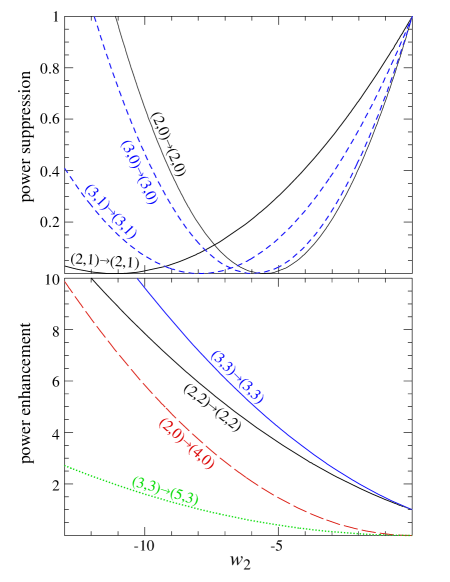
Figure 5: Multiplicative model with a quadrupolar modulation. Shown is the fractional change or transfer of power from an intrinsic multipole $(\ell,m)$ to an observed $(\ell^{\prime},m^{\prime})$ or $p_{(\ell,m)\rightarrow(\ell^{\prime},m^{\prime})}^{2}$. For a modulation amplitude $-5\lesssim w_{2}\lesssim-10$, power in $\ell=2,3$ and $m=0,1$ is suppressed while that in $(\ell,m)=(2,2)$, $(3,3)$, $(4,0)$ and $(5,3)$ is enhanced. These features are seen in the WMAP TOH data of Tab. 1 and enhance the planarity and alignment of the quadrupole and octopole.

IV Multiplicative Isotropy Breaking

A multiplicative model for breaking statistical isotropy eliminates the two fundamental flaws of the additive model. Firstly, though the modulation is still azimuthally symmetric it affects multipole moments of all $m$ values. Secondly, the change in the observed multipole moments is correlated with the intrinsic anisotropy and hence can explain alignments of power deficits. Together these features can explain the planarity and alignment of the quadrupole and octopole seen in WMAP.

Based on the instrumental example of a calibration error that varies across the sky (§IV.1), we construct a proof of principle model (§IV.2) that solves the quadrupole and octopole mutual alignment problem (§IV.3).

IV.1 Instrumental Example

An instrument whose calibration varies across the sky will modulate the intrinsic anisotropy $B(\hat{\bf n})$ as

$$T(\hat{\bf n})=f[1+w(\hat{\bf n})]B(\hat{\bf n})\,,$$ (41)

where $f$ is the sky averaged calibration and $w$ is the fluctuation in the calibration. A calibration fluctuation can transfer power from one multipole moment to another as well as alter the power in a given multipole.

Consider for a calibration fluctuation that is purely quadrupolar in nature

$$w(\hat{\bf n})=w_{2}Y_{20}(\hat{\bf n})\,.$$ (42)

This form is motivated by the need to suppress fluctuations along both poles of the preferred axis. It also relates multipoles of $\Delta\ell=2$ by Eq. (13) (see also Prunet et al. (2005) for a dipolar example) which as we will see has interesting implications for alignments and parity anomalies beyond the quadrupole and octopole Land and Magueijo (2005a, c).

The effect of this calibration modulation is an $\ell$ and $m$ dependent alteration of the amplitude of the temperature field as well as a transfer of fluctuations between $\Delta\ell=2$ modes of the same $m$. From Eq. (7), the contribution from an intrinsic fluctuation $b_{\ell^{\prime}m^{\prime}}$ to an observed multipole moment $t_{\ell m}$ is given by

$$fb_{\ell^{\prime}m^{\prime}}p_{(\ell^{\prime},m^{\prime})\rightarrow(\ell,m)}\,,$$ (43)

where

$$p_{(\ell^{\prime},m^{\prime})\rightarrow(\ell,m)} = \left(\delta_{\ell\ell^{\prime}}+R_{\ell m}^{2\,\ell^{\prime}}\right)\delta_{mm^{\prime}}\,.$$ (44)

These square of several of these $p$’s are plotted as a function of $w_{2}$ in Fig. 5. For certain values of $w_{2}$, the modulation can suppress specific multipoles of the quadrupole and octopole to zero. Interestingly for $-10\lesssim w_{2}\lesssim-5$, the suppression is efficient for $m=0,\pm 1$. Moreover for this range, the power in $\ell=2$, $m=\pm 2$ and $\ell=3$, $m=\pm 3$ is actually enhanced. These properties are exactly what is needed to explain the observed power distribution of the WMAP sky.

Furthermore, a modulation in this regime also enhances power in $\ell=4$, $m=0$ from intrinsic power in $\ell=2$, $m=0$ and $\ell=5$, $m=3$ from $\ell=3$, $m=3$. The WMAP multipoles $(4,0)$ and $(5,3)$ have excess power in the dipole direction. Finally the modulation correlates the observed signal between these pairs of multipoles. The correlation for $\ell=2$, $m=0$ is not very relevant since its observed value is consistent with noise (see Tab. 1). For $\ell=3$, $m=3$ it is of the right sign to account for enhanced fluctuations in both multipoles as seen in the WMAP data Land and Magueijo (2005a).

Unfortunately a simple calibration error cannot literally be the cause of alignments. In the discussion above we have only considered the modulation of intrinsic power in the quadrupole and octopole. A calibration error would modulate all of the intrinsic anisotropy. In this case terms such as $p_{(4,0)\rightarrow(2,0)}$ would generate observed quadrupole power out of intrinsic $\ell=4$ fluctuations and spoil the ability to lower its power.

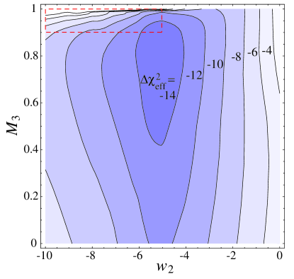
Figure 6: $\Delta\chi_{\rm eff}^{2}\equiv-2\Delta\ln{\cal L}$ for the multiplicative model with the dipole as the preferred axis. Models with $w_{2}\sim-5$ and $M_{3}\approx 0.8$ have $\Delta\chi_{\rm eff}^{2}\approx-16$ and best match the dipole frame data given that the most anomalous power deficit is in $\ell=2$, $m=0$ (see Fig. 5). The amplitude $f$ is set to minimize $\Delta\chi_{\rm eff}^{2}$ for each model. A range of models around the maximum improve the $\Delta\chi_{\rm eff}^{2}$ and most of the improvement is due to the breaking of statistical isotropy through the single parameter $w_{2}$. The dashed box highlights models which best produce angular momentum alignments in Fig. 7.

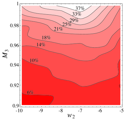
Figure 7: Percentage of multiplicative models that exhibit a higher aligned angular momentum statistic $\hat{L}^{2}$ for the quadrupole and octopole than WMAP. Here $f$ is chosen to minimize the $\Delta\chi^{2}_{\rm eff}$ of the data in the dipole frame. The percentage peaks at 45% for $w_{2}\approx-7$ and $M_{3}=1$ and is to be compared with 0.22% for the fiducial model.

IV.2 Proof of Principle Example

At least in principle, a cosmological version of the calibration mechanism has the ability to modulate only the quadrupole and octopole. Large scale temperature anisotropies can arise from both the Sachs-Wolfe and integrated Sachs-Wolfe effect and each can carry extra degrees of freedom from isocurvature fluctuations or multiple sources of curvature fluctuations. It is possible then that the presence of a long wavelength field gradient modulates only one of these effects.

Constructing a fully physical model is beyond the scope of this paper. Here we seek only a proof of principle that a multiplicative modulation of the intrinsic anisotropy can explain the WMAP anomalies. This proof of principle should help to guide the construction of an physical model that satisfies the observational requirements.

Let us take the general form for the modulation Eq. (3) where the anisotropy is constructed out of two contributions $A(\hat{\bf{n}})$ and $B(\hat{\bf{n}})$, only one of which is modulated. Based on the discussion of calibration error in the previous section, we parameterize their underlying power spectra as

$$C_{\ell}^{aa} = (1-M_{\ell})C_{\ell}^{\rm fid}\,,$$

$$C_{\ell}^{ab} = 0\,,$$

$$C_{\ell}^{bb} = M_{\ell}C_{\ell}^{\rm fid}\,.$$ (45)

Here $C_{\ell}^{\rm fid}$ is the fiducial cosmological model specified in §III.2. We will further take the modulation to be purely quadrupolar in nature as given by Eq. (42). As discussed in §III.2, a nearly pure quadrupolar modulation can be achieved in physical space by the combination of a long wavelength spatial modulation whose phase corresponds to a nearly even parity when projected on the sky.

The multiplicative modulation model is then specified by three quantities: $w_{2}$ which controls the relative amplitude of the modulation in the field $B(\hat{\bf{n}})$, $f$ which describes the relative amplitude of $A(\hat{\bf{n}})$ and $B(\hat{\bf{n}})$ contributions and $M_{\ell}$ which describes their relative contribution to each multipole moment. Given the discussion above, we seek a model where the intrinsic anisotropy is maximally modulated for the quadrupole and minimally modulated beyond the octopole. Note that the model is constructed so that in the absence of modulation ($w_{2}=0$) $C_{\ell}=C_{\ell}^{\rm fid}$ for $f=1$. Hence for simplicity we set $M_{2}=1$ and $M_{\ell\geq 4}=0$. The proof of principle model is then defined by three parameters $w_{2}$, $M_{3}$, and $f$.

IV.3 Power Deficits and Alignments

We now assess whether the WMAP data favor such a multiplicative modulation. We again begin by considering the likelihood

$${\cal L}({\bf t}|{\bf C}) = {1\over(2\pi)^{N/2}\sqrt{{\rm det{\bf C}}}}\exp\left[-{1\over 2}{\bf t}^{\dagger}{\bf C}^{-1}{\bf t}\right]$$ (46)

$$\equiv \exp[-\chi_{\rm eff}^{2}/2]$$

where ${\bf t}$ is an $N$ element vector of the WMAP TOH multipole moments $t_{\ell m}$ in the dipole direction. ${\bf C}$ is the sum of the signal covariance matrix in Eq. (13) and a diagonal noise covariance given by $N_{\ell}$ in Tab. 1. The signal covariance matrix is parameterized by $w_{2}$, $M_{3}$ and $f$ [see Eqs. (13) and (45)]. It is important here to include $N_{\ell}$ since some of the multipole moments are consistent with noise and the model has the ability to lower the predicted power in certain multipoles to zero. On the other hand an accurate quantification of noise is not crucial.

In Fig. 6, we show the improvement in $\Delta\chi_{\rm eff}^{2}$ relative to the fiducial model as a function of $(w_{2},M_{3})$ for the value of $f$ that maximizes the likelihood. The maximum likelihood value at $w_{2}=-5.0$ and $M_{3}=0.82$ has a $\Delta\chi^{2}_{\rm eff}=-16$. Even more striking, most of the gain comes through $w_{2}$. The best unmodulated or statistically isotropic model (restricted to $w_{2}=0$) has only an improvement of $\Delta\chi^{2}_{\rm eff}\approx-5$. Note that in this case maximization over $(f,M_{3})$ corresponds to the a maximization over $(C_{2},C_{3})$. The maximum at $w_{2}=-5.0$ is driven by the most anomalously low multipole moment in the dipole direction $\ell=2$, $m=0$ as shown in Fig. 5. Note however that a wide range of values surrounding the maximum would also improve the fit.

To test the quadrupole-octopole alignment, we take the normalized angular momentum (de Oliveira-Costa et al., 2004) as generalized by Ref. (Copi et al., 2005)

$$\hat{L}^{2}_{\ell}\equiv{\sum_{m=-\ell}^{\ell}m^{2}|a_{\ell m}|^{2}\over\ell^{2}\sum_{m=-\ell}^{\ell}\left|a_{\ell m}\right|^{2}}\,.$$ (47)

The statistic

$$\hat{L}^{2}\equiv{1\over 2}\left(\hat{L}^{2}_{2}+\hat{L}^{2}_{3}\right)\,$$ (48)

maximized over direction of the preferred axis captures both the alignment of the quadrupole and octopole and the planar nature of the octopole. Using Eqs. (17) and (47) and maximizing over direction, we find the best fit axis to be

$$l=247\hbox{$.\!\!^{\circ}$}3,\quad b=59\hbox{$.\!\!^{\circ}$}7$$ (49)

in galactic coordinates. This is close to but differs from the direction of the dipole $(l=263\hbox{$.\!\!^{\circ}$}85\pm 0\hbox{$.\!\!^{\circ}$}1,b=48\hbox{$.\!\!^{\circ}$}25\pm 0\hbox{$.\!\!^{\circ}$}04)$ Bennett et al. (2003a). For WMAP $\hat{L}^{2}_{\rm WMAP}=0.96$.

To assess whether the multiplicative modulation improves the probability of alignments, we draw Monte Carlo realization of the models. With the fiducial model only $0.22\%$ of $10^{4}$ realizations had a $\hat{L}^{2}>\hat{L}_{\rm WMAP}^{2}$ in any direction. For the multiplicative modulation models, the fraction of $10^{3}$ realizations is shown in Fig. 7. Here $f$ is fixed to minimize $\Delta\chi_{\rm eff}^{2}$ for each $(w_{2},M_{3})$ in the dipole direction

This fraction is maximized at $w_{2}=-7$ and $M_{3}=1$ at 45%, an increase of a factor of $\sim 200$ over the fiducial model. From Fig. 5, we see that $w_{2}=-7$ achieves the best balance of reducing the power in all moments of the quadrupole and octopole except $m=\pm\ell$. Hence such a model would be expected to produce the highest normalized angular momentum. In Fig. 8 we show an example of one of these realizations (with $\hat{L}^{2}=0.99$) that illustrates how the modulation takes an intrinsically isotropic sky into one that exhibits the alignments of WMAP.

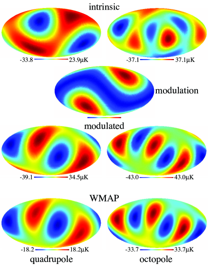
Figure 8: A realization of the multiplicative model where the quadrupole (left column) and octopole (right column) exhibit an alignment similar to WMAP. First row: intrinsic (unmodulated) sky from a Gaussian random isotropic realization. Second row (single column): the quadrupolar modulation $\propto-[1-7Y_{20}(\hat{\bf n})]$ in the dipole direction. Third row: the modulated sky of the observed CMB (with $M_{3}=1$). Fourth row: WMAP full-sky quadrupole and octopole.

Moreover, we have verified that models that solve the alignment problems do so irrespective of which test is used to quantify them. For example, the aforementioned model with $w_{2}=-7$ and $M_{3}=1$ makes the mutual closeness of the quadrupole and octopole area vectors (Schwarz et al., 2004; Copi et al., 2005) unlikely at 37% level, compared to 0.12% level without modulation.

The alignment statistic also favors high values of $M_{3}$ since $M_{2}=M_{3}=1$ implies that all contributions to the quadrupole and octopole are modulated. The $\chi^{2}_{\rm eff}$ statistic slightly disfavors very high values since in the dipole direction there remains a substantial amount of power in $\ell=3$, $m=\pm 1,\pm 2$ which is better fit with an uncorrelated isotropic component (see Tab. 1). Nonetheless there is a range of models around $w_{2}=-7$ and $M_{3}=0.95$ that both improve $\chi^{2}_{\rm eff}$ and produce a fraction of more extremely aligned skies of $>10\%$.

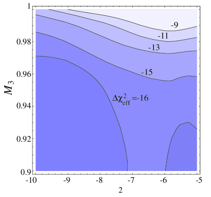
Figure 9: Same as Fig. 6 except replacing the dipole as the preferred axis with that of $\hat{L}_{\rm max}^{2}$. By maximizing the planarity of the quadrupole and octopole $|m|<\ell$ modes are minimized allowing for smaller $w_{2}$ and higher $M_{3}$.

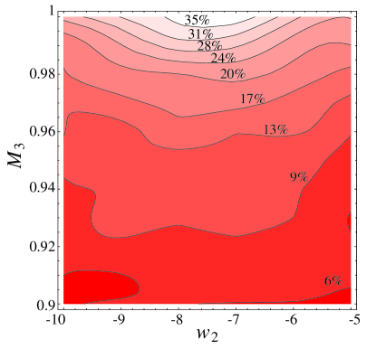
Figure 10: Same as in Fig. 7 except with $f$ given by the minimum $\Delta\chi^{2}_{\rm eff}$ in the $\hat{L}_{\rm max}^{2}$ direction. Alignment requirements remain largely unchanged from the dipole direction but maximum percentages are more compatible with substantial improvements in $\Delta\chi^{2}_{\rm eff}$ from Fig. 9.

In fact, even better models can be found if so desired. Choosing the preferred axis to be exactly the dipole for parameter fitting is not necessary. In fact in the $\hat{L}_{\rm max}^{2}$ direction of WMAP (see Eq. (49)) the planarity of the observed quadrupole and octopole is maximized and hence has particularly low $m=\pm 1$, $m=\pm 2$ components (see Tab. 1). Fitting parameters of the model to the data with this as the preferred axis allows a wider range of solutions (see Fig. 9). Now models with more negative $w_{2}$ are favored to reduce the power in these components and higher values of $M_{3}$ are allowed. With the maximum likelihood $f$ values with this preferred axis, $w_{2}=-7$ and $M_{3}\approx 1$ still produces more extreme alignments in $\sim 45\%$ of the Monte Carlos. Moreover models exist with $\chi^{2}_{\rm eff}$ improvements of more than $-10$ which produce alignments more extreme than WMAP in $\gtrsim 30\%$ of the Monte Carlos (see Fig. 10).

The change in $\Delta\chi^{2}_{\rm eff}$ between the dipole and $\hat{L}_{\rm max}^{2}$ directions and more generally its sensitivity to direction indicates that one should be careful in interpreting this improvement probabilistically. A $\Delta\chi^{2}_{\rm eff}\approx-16$ likelihood improvement naively suggests a “4-$\sigma$” result. However since the choice of the $\hat{L}_{\rm max}^{2}$ direction maximizes the planarity of the quadrupole and octopole, there will be some preference for modulation even for realizations of a statistically isotropic sky.

To address this issue, we fit the model parameters in the $10^{4}$ realizations of the isotropic fiducial model in the $\hat{L}_{\rm max}^{2}$ direction of each run. We find that the WMAP measured sky shows a greater improvement in the likelihood than 98.8% of the Gaussian random, isotropic skies indicating that the multiplicative model is indeed strongly preferred by the WMAP observations.

Since this exercise is simply a proof of principle with somewhat ad hoc parameters, we do not pursue finding the best model parameters further. The important conclusion is that models exist where a multiplicative modulation of large angle anisotropies in a quadrupolar pattern can make the WMAP alignments a likely occurrence.

V Discussion

We have introduced a general class of models that break statistical isotropy in CMB temperature fluctuations spontaneously. The key elements are a non-linear response in the CMB to long wavelength fluctuations in a mediating field. Long wavelength fluctuations pick a direction through their local gradient and a non-linear response allows this direction to be imprinted in a range of multipole moments.

We have examined two subclasses of models based on whether isotropy is broken through an additive contribution to the anisotropy or a multiplicative one. The two classes have analogues in the instrumental domain and are related to saturation in detectors and an angular drift in calibration.

As a cosmological example of the additive class, we considered gradients in a quintessence field that are non-linearly mapped through that field’s potential into dark energy density perturbations. The CMB then responds linearly to these density perturbations through the integrated Sachs-Wolfe effect. The existence of such contributions allows for the underlying CMB to be isotropic. Nonetheless, additive contributions cannot be said to solve the alignment problem in WMAP. Since the anomalies in the quadrupole and octopole are related to a deficit of power near the dipole direction, an additive correction can only explain the observations if the intrinsic fluctuations cancel them in both. This is statistically less likely than having an aligned deficit of power by chance without isotropy breaking.

This fundamental problem exists for all explanations of the alignments which seek to restore power to the CMB including those involving foregrounds or other uncorrelated templates. Additionally, an additive contribution based on an azimuthally symmetric modulation of a gradient field can only affect $m=0$ multipoles around the preferred axis. The only remaining possibility is that the additive contributions themselves account for most of the power in the quadrupole and octopole. All of the moments of the intrinsic quadrupole and octopole would then be even lower than those observed, exacerbating the power deficit problem.

These difficulties can be overcome by a model which breaks isotropy multiplicatively. Here we have demonstrated a proof of principle that the alignments and power distribution of WMAP can be made likely with such a mechanism. By modulating the intrinsic quadrupole and octopole in a quadrupolar fashion, the likelihood of the WMAP data can be increased by a factor of $e^{16/2}$ and separately, the probability of obtaining a sky with a higher angular momentum statistic is increased by $200$ to $\sim 45\%$. The angular momentum statistic is a quantification of both the planarity of the octopole and its alignment with the quadrupole. Note that the likelihood increase must be considered in the context of the directional maximization of the angular momentum. The fiducial isotropic model would falsely produce greater than $e^{16/2}$ improvements in $\sim 1\%$ of realizations.

In addition, the model predicts correlated power excess power in $\ell=3$, $m=3$ and $\ell=5$, $m=3$ and more generally the $\Delta\ell=2$ parity pattern of anomalies in the data Land and Magueijo (2005c). There is a range of parameters that jointly increase the likelihood by $e^{10/2}$ and the angular momentum probability to $\sim 30\%$.

There are also classes of anomalies that are not explained by this version of spontaneous isotropy breaking. Solar system related alignments (Schwarz et al., 2004; Copi et al., 2005) and the asymmetry in power between the northern and southern ecliptic ecliptic hemisphere (Eriksen et al., 2004b) both fall into this category. While isotropy breaking involving a dipolar modulation Prunet et al. (2005) along the ecliptic could potentially explain the latter feature, it cannot simultaneously explain anomalies along the dipole direction. Furthermore, there is no fundamental link between the dipole of our peculiar motion and the preferred axis for symmetry breaking. That coincidence remains in the multiplicative model.

We emphasize that this proof of principle is not a physical model and challenges will have to be overcome in constructing one. The level of multiplicative modulation preferred is fairly extreme and cannot be considered a perturbation. It must affect essentially all of the quadrupole and octopole in spite of the fact that in the fiducial cosmology there are two physically distinct sources to these fluctuations: the Sachs-Wolfe and ISW effects. Thus a physical solution will have to modify the power spectrum of these contributions as well. On the other hand the modulation must not continue to intrinsic fluctuations in multipoles much higher than the octopole. Thus two distinct sources of anisotropy are required.

Constructing a physical mechanism that satisfies all of these requirements will clearly be challenging and is beyond the scope of this paper. Likewise the significance of the alignments and hence the model improvements may be degraded by foreground and systematic contamination not accounted for in the all-sky cleaned maps, at the expense of exacerbating the power deficit problems. Nevertheless, this proof of principle model can serve as a guide both to building a physical model and to searching for alternate explanations of the anomalies.

Acknowledgments: CG was supported by the KICP under NSF PHY-0114422; WH by the DOE and the Packard Foundation; DH by the NSF Astronomy and Astrophysics Postdoctoral Fellowship under Grant No. 0401066; TC by NSF OPP-0130612. We have benefited from using the publicly available Healpix package Górski et al. (2005). We thank Stephan Meyer, Hiranya Peiris and Bruce Winstein for useful discussions and Craig Copi for providing a Wigner rotation matrix code. WH thanks the WMAP team for supplying the “beach ball” representation of the data.

References

- Bennett et al. (2003a) C. L. Bennett et al., ApJS 148, 1 (2003a).
- Smoot et al. (1992) G. F. Smoot et al., Astrophys. J. Lett. 396, L1 (1992).
- Efstathiou (2004) G. Efstathiou, MNRAS 348, 885 (2004), eprint astro-ph/0310207.
- Slosar et al. (2004) A. Slosar, U. Seljak, and A. Makarov, Phys. Rev. D69, 123003 (2004), eprint astro-ph/0403073.
- Bielewicz et al. (2004) P. Bielewicz, K. M. Górski, and A. J. Banday, MNRAS 355, 1283 (2004), eprint astro-ph/0405007.
- O’Dwyer et al. (2004) I. J. O’Dwyer et al., Astrophys. J. 617, L99 (2004), eprint astro-ph/0407027.
- Tegmark et al. (2003) M. Tegmark, A. de Oliveira-Costa, and A. J. Hamilton, Phys. Rev. D68, 123523 (2003).
- de Oliveira-Costa et al. (2004) A. de Oliveira-Costa, M. Tegmark, M. Zaldarriaga, and A. Hamilton, Phys. Rev. D69, 063516 (2004), eprint astro-ph/0307282.
- Copi et al. (2004) C. J. Copi, D. Huterer, and G. D. Starkman, Phys. Rev. D70, 043515 (2004).
- Schwarz et al. (2004) D. J. Schwarz, G. D. Starkman, D. Huterer, and C. J. Copi, Phys. Rev. Lett. 93, 221301 (2004), eprint astro-ph/0403353.
- Land and Magueijo (2005a) K. Land and J. Magueijo, astro-ph/0502237 (2005a), eprint astro-ph/0502237.
- Land and Magueijo (2005b) K. Land and J. Magueijo, astro-ph/0502574 (2005b), eprint astro-ph/0502574.
- Slosar and Seljak (2004) A. Slosar and U. Seljak, Phys. Rev. D70, 083002 (2004), eprint astro-ph/0404567.
- Copi et al. (2005) C. J. Copi, D. Huterer, D. J. Schwarz, and G. D. Starkman (2005), eprint astro-ph/0508047.
- Hinshaw et al. (2003) G. Hinshaw et al., Astrophys. J. Suppl. 148, 63 (2003), eprint astro-ph/0302222.
- Bennett et al. (2003b) C. L. Bennett et al., ApJS 148, 97 (2003b), eprint astro-ph/0302208.
- Finkbeiner (2004) D. P. Finkbeiner, Astrophys. J. 614, 186 (2004), eprint astro-ph/0311547.
- Bielewicz et al. (2005) P. Bielewicz, H. K. Eriksen, A. J. Banday, K. M. Górski, and P. B. Lilje, astro-ph/0507186 (2005), eprint astro-ph/0507186.
- Varshalovich et al. (1988) D. A. Varshalovich, A. N. Moskalev, and V. K. Khersonskii, Quantum Theory of Angular Momentum (World Scientific, 1988).
- Eriksen et al. (2004a) H. K. Eriksen, A. J. Banday, K. M. Górski, and P. B. Lilje, Astrophys. J. 612, 633 (2004a), eprint astro-ph/0403098.
- Gordon and Hu (2004) C. Gordon and W. Hu, Phys. Rev. D 70, 083003 (2004), eprint astro-ph/0406496.
- Hu and Eisenstein (1999) W. Hu and D. J. Eisenstein, Phys. Rev. D59, 083509 (1999), eprint astro-ph/9809368.
- Jaffe et al. (2005) T. R. Jaffe, A. J. Banday, H. K. Eriksen, K. M. Górski, and F. K. Hansen (2005), eprint astro-ph/0503213.
- Prunet et al. (2005) S. Prunet, J.-P. Uzan, F. Bernardeau, and T. Brunier, Phys. Rev. D71, 083508 (2005), eprint astro-ph/0406364.
- Land and Magueijo (2005c) K. Land and J. Magueijo (2005c), eprint astro-ph/0507289.
- Eriksen et al. (2004b) H. K. Eriksen, F. K. Hansen, A. J. Banday, K. M. Górski, and P. B. Lilje, Astrophys. J. 605, 14 (2004b), eprint astro-ph/0307507.
- Górski et al. (2005) K. M. Górski, E. Hivon, A. J. Banday, B. D. Wandelt, F. K. Hansen, M. Reinecke, and M. Bartelmann, Astrophys. J. 622, 759 (2005).