GRB afterglow light curves in the pre-Swift era – a statistical study

Abstract

We present the results of a systematic analysis of the world sample of optical/near-infrared afterglow light curves observed in the pre-Swift era by the end of 2004. After selecting the best observed 16 afterglows with well-sampled light curves that can be described by a Beuermann equation, we explore the parameter space of the light curve parameters and physical quantities related to them. In addition, we search for correlations between these parameters and the corresponding gamma-ray data, and we use our data set to look for a fine structure in the light curves.

1 Introduction

Nearly ten years after the discovery of the first Gamma-Ray Burst (GRB) afterglow in the optical/near-infrared (Groot et al., 1997; van Paradijs et al., 1997), the progress in the understanding of the GRB phenomenon is enormous (e.g., Zhang & Mészáros, 2004; Piran, 2005). From the observational point of view nearly every individual afterglow has turned out to be specific in some sense. The richness in afterglow properties observed so far is not much surprising, however, given the fact that the afterglow phenomenon combines internal properties of the underlying burster population with properties of the external circumburster medium. This in combination with redshift provides a large parameter space for various flavors of GRB afterglows. However, in spite of their individualities, as an ensemble afterglows trace the underlying physical boundary conditions and the parameter space of the physical processes involved. Revealing this parameter space is of fundamental interest since it might much improve the understanding of the afterglow phenomenon. This has already motivated several groups to perform a systematic analysis of observational data from various afterglows (e.g., Frontera et al., 2000; Panaitescu & Kumar, 2001a, b, 2002; Yost et al., 2003; Frail et al., 2003a, 2004; Stratta et al., 2004; Gendre & Boër, 2005; Panaitescu, 2005a, b). The present work continues this kind of investigations but concentrates on the optical/NIR bands.

While a fit of the observed broad-band spectral energy distribution (SED) of an afterglow from the radio to the X-ray band is the best way in order to extract the underlying physical parameters (e.g., Frail et al., 2003b; Yost et al., 2002; Panaitescu, 2005b), one might expect that the optical/NIR data alone are completely explainable within the context of the underlying theoretical model. In particular, in most cases it is the optical/NIR region where the sampling and the quality of the afterglow data is best. It is clear that any reliable theoretical model must be able to explain the observed richness in the phenomenology of optical light curves of GRB afterglows. In this respect it is worth summarizing and exploring the available data base on afterglows in the optical/NIR bands. This holds in particular with respect to the new era in GRB research initiated by the launch and operation of the Swift satellite (Gehrels, 2004).

In the present paper we continue our systematic analysis of afterglow parameters based on optical and near-infrared data (Zeh, Klose, & Hartmann 2004, hereafter Paper I; Zeh, Klose, & Hartmann 2005). Our study includes $all$ afterglows in the pre-Swift era with sufficient published data. While in Paper I we analyzed the afterglow light curves with special emphasis on an underlying supernova component, the goal of the present paper is to explore the parameter space of the light curve parameters and of physical quantities related to them. In Paper III (Kann, Klose, & Zeh, 2005), we expand this analysis to the spectral energy distribution of afterglows in the optical and near-infrared bands in order to search for signatures of dust in GRB host galaxies.

2 Data analysis

We collected from the literature all available photometric data on GRB afterglows observed by the end of 2004 and checked them for consistency. We modeled the light curve of the optical transient (OT) following a GRB as a composite of genuine afterglow light, supernova (SN) light, and constant light from the underlying host galaxy. The afterglow is either modeled by a single or a smoothly broken double power-law according to Beuermann et al. (1999). Our fitting procedure is based on a $\chi^{2}$ minimization with a Levenberg-Marquardt iteration. This minimization technique provides formal uncertainties of the fitted parameters through the covariance matrix. For the remainder of this paper, all uncertainties are 1$\sigma.$

We always fitted photometric magnitudes with a fitting equation as follows:

$$m_{\rm OT}(t) = -2.5\,\log\{10^{-0.4\,m_{c}}[(t/t_{\rm b})^{\alpha_{1}\,n}+(t/t_{\rm b})^{\alpha_{2}\,n}]^{-1/n}$$ (1)

$$+ k\,10^{-0.4\,m_{\rm SN}(t/s)}+10^{-0.4\,m_{\rm host}}\}\,.$$

The parameters in Equation (1) are the prebreak decay slope $\alpha_{1}$, the postbreak decay slope $\alpha_{2}$, the break time $t_{\rm b}$, the steepness of the break $n$, the brightness of the host galaxy $m_{\rm host}$, the constant $m_{c}$ which corresponds to the magnitude of the fitted light curve for the case $n=\infty$ at the break time $t_{\rm b}$ (it stands for the intersection point of the prebreak and the postbreak slope, without considering a smooth transition), as well as the supernova parameters $k$ and $s$, which indicate the luminosity ratio and the stretch factor normalized to SN 1998bw (cf. Paper I). If there is no break in the light curve, then Equation (1) reduces to

$$m_{\rm OT}(t) = -2.5\,\log\{10^{-0.4\,m_{1}}t^{\alpha}$$ (2)

$$+ k\,10^{-0.4\,m_{\rm SN}(t/s)}+10^{-0.4\,m_{\rm host}}\}\,,$$

where $m_{1}$ is the brightness of the afterglow at $t=1$ day after the burst. Before the fitting process the data were corrected for Galactic extinction using the maps of Schlegel, Finkbeiner, & Davis (1998). For a more detailed description of our procedure we refer to Paper I.

In the present paper, our input list contains 59 optical/NIR afterglows observed in the pre-Swift era which allowed us to perform a fit (Table 1). Sixteen of these have a well-sampled light curve in at least one photometric band (mostly the $R_{C}$ band). These light curves show a well-detectable break and have sufficient data points before and after the break time, so that the prebreak decay slope and the postbreak decay slope according to Equation (1) are well-defined. More precisely, our selection criterium for the best-defined afterglow light curves is that the $1\sigma$ error is less than 0.2 for $\alpha_{1}$, less than 0.3 for $\alpha_{2}$, and less than 1 day for $t_{b}$ (Table 1). We did not use the accuracy of the fit ($\chi^{2}$ per degrees of freedom) as a selection criterium, however. We consider Equation (1) as an empirical first order approximation of an observed light curve and all deviations from the corresponding fit as fine structure (§ 4.4). Light curves with no break are by definition excluded from this sample of best-defined afterglows, because it cannot be ascertained with complete certainty if the slope is a pre- or postbreak. Whenever we did not detect a break, the data quality was usually insufficient to exclude the possibility of a jet break in the light curve. In these cases there is either no early time data available, or the break could have been missed because of a bright host galaxy or an underlying SN component.

All but one (GRB 980519) of the 16 afterglows in our sample have a known redshift, none of these bursts is classified as an X-ray flash. For the present study the afterglows of GRB 021004 and GRB 030329 were excluded from our analysis because of their many rebrightening episodes (see also § 4.4). In the case of the afterglow of GRB 030329, we performed two additional fits that are also given in Table 1, the details are in Appendix A. While these fits give very good results, they are based on only a small part of the light curve and we thus do not include their results in the selected sample for statistical study, with the exception of Figure 8. The afterglow of GRB 000301C also shows a rebrightening episode (around 3.5 days after the burst; Garnavich, Loeb, & Stanek, 2000; Gaudi, Granot & Loeb, 2001), but as the deviations are not that large and occur only during a certain period, the light curve can still be fitted with a broken power-law, even though $\chi^{2}_{\rm d.o.f.}$ becomes relatively large.

A special note is required for GRB 021211. The afterglow light curve of this burst fulfills the aforementioned criteria for the amount of the $1\sigma$ error bars of the fit parameters, nevertheless we have not included it in our subsample of well-defined light curves. According to our data, the light curve shows a break 0.11$\pm$0.09 days after the burst with a steepening by $\Delta\alpha=\alpha_{2}-\alpha_{1}=0.26\pm 0.11$. This is in close agreement with the amount of steepening expected for the passage of the cooling break across the optical window (for a Compton parameter less than 1; e.g., Panaitescu & Kumar, 2001a). In addition, Nysewander et al. (2005) report on evidence for color changes of the afterglow just around this time. Given the fact that no optical data have been reported in the literature for the time period between 1 and 10 days after the burst, we consider it as very likely that the break in the light curve we have found does indeed signal the passage of the cooling break (as already suspected by Nysewander et al., 2005, based on their finding of color changes), while the real jet break occurred between 1 and 10 days after the burst. Note that the light curve break around 0.11 days is not identical to the break discussed by others concerning the very early light curve, which has been attributed to the reverse shock (Li et al., 2003; Fox et al., 2003; Wei, 2003; Holland et al., 2004; Kumar & Panaitescu, 2003). Given these findings, and since we try to keep our subsample as homogeneous as possible, we have not included this burst in the following study.

The light curve parameters we have deduced from our data might be slightly different to those obtained and used by other groups. This is mainly due to the fact that we use a different, and most likely larger data base. In addition, there is still some bias in the selection of the data, in the definition of what are outliers, which data should be used and which data should not. While we do not claim that our data base is the best for every individual GRB, most probably it is the most comprehensive set. The strength of our approach is that we analyze all afterglow light curves using the same numerical procedure. In this respect we are confident that the results we obtain are statistically robust.

3 Results

The results of our light curve fitting of the individual afterglows are summarized in Table 1. Here, the second column indicates the sample of the best-defined 16 afterglows. In some cases we could only derive upper or lower limits for some parameters, because the light curve was poorly sampled (see § A). In the following we discuss only the results obtained for this sample of 16 afterglows.

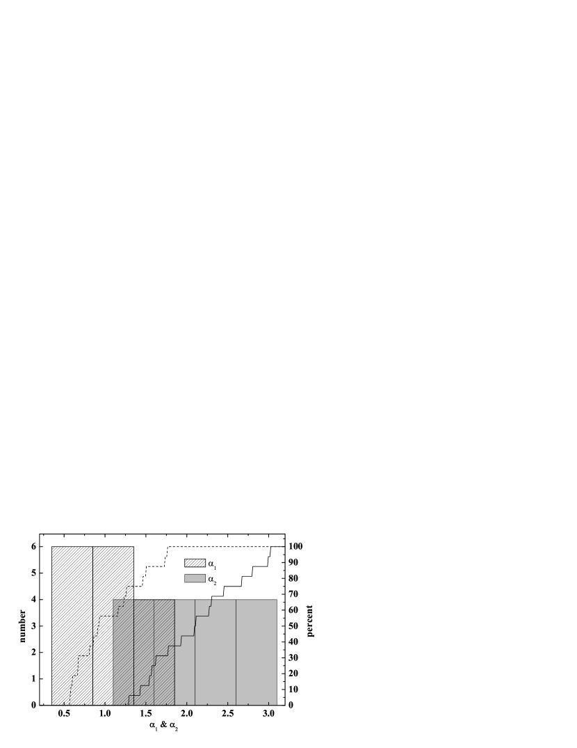
Figure 2: The distribution of the prebreak decay slope $\alpha_{1}$ and the postbreak decay slope $\alpha_{2}$ for the 16 afterglows in our sample with the best defined light curves (Table 1; bin size 0.5). The broken line and the solid line represent the cumulative distribution for $\alpha_{1}$ and $\alpha_{2}$, respectively.

The distributions of the deduced light curve parameters are shown in Figures 2 to 4. The mean of the prebreak decay slope is $\alpha_{1}=1.05\pm 0.10$, with $\alpha_{1}$ ranging from $0.58\pm 0.05$ (GRB 000301C) to $\alpha_{1}=1.76\pm 0.05$ (GRB 011121), while $\alpha_{2}$ ranges from $1.30\pm 0.02$ (GRB 041006) to $3.03\pm 0.27$ (GRB 030429) with the mean at $2.12\pm 0.14$. About half of the postbreak decay slopes have $\alpha_{2}<2.0$. Both distributions overlap in the interval from about 1.3 to 1.7. The distribution of $\alpha_{2}$ is almost constant, with a possible cutoff around 1.3 and no preference for any value.

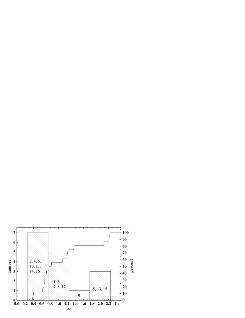
Figure 3: The distribution of the light curve steepening $\Delta\alpha=\alpha_{2}-\alpha_{1}$. The numbering follows Table 1. The solid line is the cumulative distribution.

Figure 3 displays the distribution of the difference of the decay slopes before and after the break, $\Delta\alpha=\alpha_{2}-\alpha_{1}$. The distribution is asymmetric with its maximum around 0.8 and a longer tail towards higher values. It is notably broader than the distribution of $\alpha_{1}$ and $\alpha_{2}$. It also indicates the possibility that some afterglows could have very shallow breaks with $\Delta\alpha<0.3$ that could easily be missed. The gap around $\Delta\alpha=1.7$ is probably due to low-number statistics and we do not consider it to be significant. In this respect we cannot confirm the potential evidence for a bimodality of the distribution of $\Delta\alpha$ (Panaitescu, 2005a), allthough we cannot reject this possibility either.

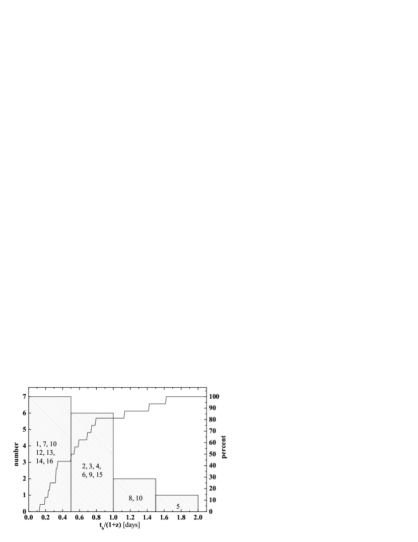
Figure 4: The distribution of the break time $t_{\rm b}$ in the GRB host frame for all bursts of our sample of 16 afterglows. The data cover the range from $t_{\rm b}/(1+z)=0.14\pm 0.02$ days (GRB 041006) to $1.62\pm 0.06$ days (GRB 000301C). Most afterglows exhibit a break at less than 1 day after the burst in the host frame. For GRB 980519 we assumed a redshift of $z=1.5$, but it would fall into the first bin even if $z=0$. The solid line represents the cumulative distribution.

In Figure 4 we present the distribution of the observed break times for the afterglows with the best-defined light curves, but translated into the corresponding GRB host frame. This distribution is strongly asymmetric with a clear peak in the host frame at lower values around 0.3 days. That most breaks occur at relatively early times supports the view that in several cases (Table 1) light curve breaks might have been missed due to a lack of early-time data. The afterglow with the earliest break in the host frame was GRB 041006, while the afterglow of GRB 000301C had the latest break time. On the other hand, late breaks might have been missed in several cases too, because the afterglow was already too faint at the break time, and/or an underlying SN component or a bright host galaxy simply made the discovery of the break in the optical bands impossible. We conclude that these data indicate, even though they do not prove, that in fact all afterglow light curves have detectable breaks due to a collimated explosion, as long as they are not hidden by rebrightening episodes as in GRB 030329 (e.g., Lipkin et al., 2004). It is clear that any model that explains the observed light curve breaks must be able to reproduce this observed distribution (Figure 4).

The distribution of the shape parameter $n$ (Equation 1) is more difficult to quantify. While for about half of the afterglows the data allowed us to determine $n$ during the fitting procedure, in the other cases $n$ did not converge during the fit ($n\rightarrow\infty$), because the sampling of the data is not good enough. It is worth noting that whenever we were able to determine $n$, we obtained a relatively soft break ($n\approx 1-2$) and in each case the prebreak decay slope $\alpha_{1}$ was very shallow. In the other cases we had to fix $n$ at a relatively large value in order to obtain an acceptable fit, and we chose $n=10$. Choosing $n\approx 1-2$ made the fit worse. Whether this indicates a possible bimodal distribution of the parameter $n$ is an open question. The distribution of the shape parameter $n$ is the biggest unknown, so far, including its theoretical interpretation.

4 Discussion

4.1 Wind versus ISM models

Figure 5 shows the correlation between the parameters $\alpha_{1}$ and $\alpha_{2}$ in comparison with eight standard afterglow models that cover the cases (1) $\nu<\nu_{c}$, (2) $\nu_{c}<\nu,Y<1$, (3) $\nu_{c}<\nu,Y>1,2<p<3$, (4) $\nu_{c}<\nu,Y>1,p>3$ for the ISM and for the wind model, where $\nu$ is the observed frequency and $Y$ is the Compton parameter (Panaitescu & Kumar, 2001a, their eqs. 21, 22 and 29). Those models with $\nu<\nu_{c}$ and $Y<1$ require $p<2$ in order to explain an observed $\alpha_{2}<2$. In particular, there is a group of five bursts (GRBs 990123, 991216, 010222, 030328, 041006) that cluster around $\alpha_{2}=1.5$. Within the corresponding 1$\sigma$ error bars $\alpha_{2}>2$ is basically ruled out and so is $p>2$. Such shallow postbreak decay slopes cannot be explained by a flat electron distribution either (Dai & Cheng, 2001; Bhattacharya, 2001; Wu et al., 2004).

Based on the underlying theoretical models, which predict $p=\alpha_{2}$, then we find that the parameter space of $p$ is rather broad, ranging from about 1.5 to 3. While the results obtained for $p$ for the individual afterglows differ among various authors, all studies agree that within the current theoretical framework no evidence for a universality of $p$ is found (e.g., Panaitescu & Kumar, 2001a, b, 2002; Preece et al., 2002; Yost et al., 2003; Panaitescu, 2005b, ;Paper III). This is contrary to what one might expect from theoretical models of highly relativistic shocks (Achterberg et al., 2001; Kirk et al., 2000), and contrary to what one might prefer on theoretical grounds (Freedman & Waxman, 2001).

If one allows for $p<2$ then an inspection of Figure 5 shows that a wind model with $\nu<\nu_{c}$ is preferred for GRBs 980519, 990123, 991216, 000926, 020124, 020405, 030328, and 041006, even though GRBs 990123, 991216 and 000926 lie fairly off the models because of their relatively small $\alpha_{2}$ or large $\alpha_{1}$. On the other hand, an ISM model with $\nu<\nu_{c}$ is preferred for GRB 990510 and GRB 011211. GRB 020813 is either an ISM case with $\nu<\nu_{c}$ or an ISM/wind case with $\nu>\nu_{c}$, in the following, we will assume this to be an ISM case. Two afterglows (GRB 010222 and GRB 011121) could be an ISM or a wind case with $\nu>\nu_{c}$. In the case of GRB 011121, the error bars are so large that $\nu<\nu_{c}$ cannot be fully excluded. Finally, the afterglows of GRBs 000301C, 030226, and 030429 are outliers because of their relatively large $\alpha_{2}$. It is noteworthy that all afterglows with soft breaks in the light curve ($n\approx 1-2$) belong to the group of bursts that are less compatible with a wind profile, and all these afterglows have $\alpha_{1}<1$.

It is difficult to quantify whether the outliers really represent a different population or whether in these cases the light curves are simply ill-defined. For example, the afterglow of GRB 000301C was affected by a strong rebrightening episode that has been modeled by a gravitational microlensing event (Garnavich, Loeb, & Stanek, 2000). As these authors note, the removal of this event leads to $\alpha_{1}\approx 1.1$, which would shift GRB 000301C toward the theoretical prediction of the ISM model with $\nu<\nu_{c}$. In the case of GRB 030226 there is evidence that the afterglow light curve showed fluctuations. In combination with the relatively sparse set of postbreak data it is well possible that the late-time observations stopped when the afterglow underwent a fluctuation, so that finally the deduced postbreak decay slope is too large. On the other hand, early-time spectra of this afterglow reveal features that can be best understood as due to a stellar wind profile (Klose et al., 2004). In the case of 030429, Jakobsson et al. (2004b) find that the light curve undergoes a significant rebrightening around 1.7 days after the burst. They suggest to exclude the data around the rebrightening from the fit and fix $\alpha_{2}=1.7$ (deduced from the SED and the $\alpha-\beta$ relations). In this case the light curve would be compatible with an ISM/wind model and $\nu>\nu_{c}$, although it is unclear how large the error in $\alpha_{2}$ would be.

If we neglect GRBs 000301C, 030226, and 030429, then Figure 5 shows that the group of optical afterglows that is compatible with a wind model is notably larger than the group of afterglows that prefers an ISM model. While basically all studies in the literature agree that afterglows seem to separate into a group that can be best described by a wind model and a group that can be best described by an ISM model, our data show that the wind scenario is statistically preferred. In fact, within their 1$\sigma$ error bars nearly all $(\alpha_{1},\alpha_{2})$ pairs are compatible with a wind profile while for the ISM model such a statement is clearly ruled out.

4.2 The jet opening angles

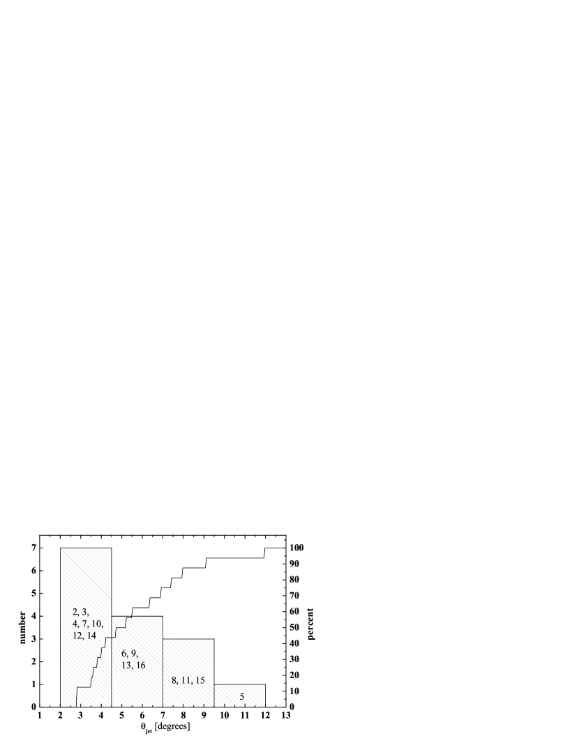
Figure 6: The distribution of the derived jet half-opening angle, $\theta_{\rm jet}$, of our sample (§ 4.2). GRB 980519 is not included here since its redshift is not exactly known.

Figure 6 displays the distribution of the jet half-opening angle, $\theta_{\rm jet}$, for our sample of 16 bursts (GRB 980519 is not included as no redshift of this burst is known) as derived from the observed break time, assuming the uniform jet model (Rhoads, 1999). We calculated $\theta_{\rm jet}$ following Sari, Piran, & Halpern (1999) for an ISM medium (GRBs 990510, 000301C, 011211, 020813, 030226, 030429) and Bloom, Frail & Kulkarni (2003) for a wind-like medium (GRBs 990123, 991216, 000926, 010222, 011121, 020124, 020405, 030328, 041006), according to the results obtained for the density profile of the individual afterglows (§ 4.1). For the isotropic equivalent energy $E_{\rm iso}$, the radiation efficiency and the redshift we adopted the values given by Friedman & Bloom (2005). In the case of an ISM model we used the circumburster density as given in Friedman & Bloom (2005), while for the wind model we assumed a mass-loss rate to wind speed ratio of $A_{*}=1$ (cf. Chevalier & Li, 2000). The distribution of $\theta_{\rm jet}$ that we have found is strongly asymmetric with a peak between 2 and 5 degrees, has a lower cutoff around 2 degrees and rapidly falls towards larger angles, in agreement with what has been found in previous studies (Frail et al., 2001; Panaitescu & Kumar, 2001b, 2002; Bloom, Frail & Kulkarni, 2003).

4.3 Correlations

Using the derived jet half-opening angles (§ 4.2) we find that the distribution of the beaming corrected energy release in the gamma-ray band ranges from $E_{\rm cor}=10^{49.9}$ erg (GRB 041006) to $E_{\rm cor}=10^{51.4}$ erg (GRB 990123). In combination with the corresponding peak energies, $E_{\rm peak}$, in the gamma-ray band (Friedman & Bloom, 2005), in Figure 7 we plot the correlation between $E_{\rm cor}$ and $E_{\rm peak}$ in the GRB host frame, as it was first reported by Ghirlanda, Ghisellini & Lazzati (2004). Considering bursts #9 and #12 as outliers and excluding them from the fit, we find $E_{\rm peak}\simeq 748\,(E_{\rm 51,cor})^{\eta}$, with $\eta=0.79\pm 0.09$. This is in qualitative agreement with Ghirlanda et al. (2004) as well as Dai, Liang & Xu (2004). On the other hand, there are differences, in particular concerning the existence of the two outliers. They can be understood, however, since the fit includes assumptions about the gas density in the GRB environment, which enters the calculation of the jet opening angle. We made use of the values provided by Friedman & Bloom (2005) and these are higher by a factor of 10/3 compared to the values used by Ghirlanda et al. (2004). In addition, in several cases the gamma-ray data given in Friedman & Bloom (2005) are notably different from those used by Ghirlanda et al. (2004). Additionally, we also considered a wind-like circumburst medium for some cases to calculate the jet half-opening angle, while Ghirlanda et al. (2004) only regard an ISM-like circumburst medium. It is therefore not surprising that we do not exactly reproduce their results (for a discussion, see also Friedman & Bloom 2005). For instance, if we reduce the assumed circumburster gas density for bursts #9 and #12 from 10 to 1 cm^-3, then the corresponding data points do not fall out of the sample anymore. A fit then provides $\eta=0.78\pm 0.09$. While our data base is too small in order to investigate the role of outliers in the Ghirlanda relation, we note that also the relation between the isotropic equivalent energy release in the gamma-ray band and the intrinsic peak energy (Amati et al., 2002) is not very tight. In a recent study on BATSE GRBs, Nakar & Piran (2005) find that about 25% of all bursts do substantially deviate from this empirical relation (see also Band & Preece, 2005).

In addition to the Ghirlanda relation, we have searched for linear correlations between all individual afterglow parameters and between the burst parameters in the gamma-ray band and the corresponding afterglow parameters. Table 2 lists the corresponding correlation coefficients derived from weighted linear fits. The Ghirlanda relation (here including the two outliers discussed above) is between $\log(E_{\rm cor})$ and $\log(E_{\rm peak})$. Relatively tight correlations between $\theta_{\rm jet}$ and $t_{b}/(1+z)$ and between $\theta_{\rm jet}$ and $\log E_{\rm cor}$ are expected, as $\theta_{\rm jet}$ derives from $t_{b}/(1+z)$ and $\log E_{\rm cor}$ derives from $\theta_{\rm jet}$. Note that the correlations for the wind model are much tighter than for the ISM model, giving further significance to the statistical conclusion that most circumburst environments are wind-blown (§ 4.1). Next to the Ghirlanda relation and the others just discussed, there are more correlations that seem significant according to the absolute correlation coefficient, but visual inspection does not support this conclusion. This holds also for the potential correlation between $\theta_{\rm jet}$ and $\alpha_{1}$ which has been reported for X-ray data (Liang, 2004). Still, it is interesting to note that $\alpha_{2}$ seems more or less correlated with all other parameters, including the redshift. On the other hand, $\theta_{\rm jet}$, $\log E_{\rm cor}$ and $\log E_{\rm peak}$ are completely uncorrelated with the redshift. We conclude that no evolutionary effect in the initial explosion parameters is evident over a wide range of redshifts.

Of special interest is the parameter $n$, which indicates the smoothness of the break (Equation 1). Even though we could only determine $n$ for a few afterglows, it looks suspicious that each time we had to fix $n$ to a relatively high value in order to get an acceptable fit, the prebreak decay slope is $\alpha_{1}>1$. To test if this could be due to a numerical problem we reconsidered the afterglow light curve of GRB 030329 and fitted it only between 0.28 and 1 days, which includes the time around the supposed jet break (e.g., Uemura et al., 2003) but excludes the cooling break (Sato et al., 2003) and the rebrightening episodes (e.g., Lipkin et al., 2004). For this time period the data density is high enough in order to deduce a value for $n$ even if the break is very sharp. Indeed, in this case we find $\alpha_{1}=1.17\pm 0.01,t_{b}=0.68\pm 0.02$ days, $\alpha_{2}=2.21\pm 0.07$ and $n=7.54\pm 1.47$. Adding this to our sample of afterglows with a deduced parameter $n$ (Table 1), a weak trend between $n$ and $\alpha_{1}$ becomes apparent (Fig. 8). It indicates that a shallow prebreak decline leads to a smooth break or, seen the other way around, a smooth break (a ”rollover”) implies a shallow prebreak decay slope. As we only have very few values of $n$, we do not regard this as strong statistical evidence for a correlation, since an observational bias cannot be excluded. Afterglows with a shallow decay are bright for a longer period of time, which makes them easier to follow. Therefore, the data density around the break time is usually higher compared to most afterglows with a steep decline. A high data density around the break time is essential to determine a value for $n$, however. Nevertheless, it is worth to check if this trend is confirmed in the Swift-era.

Unfortunately, most bursts in our sample are at high redshift, so that no supernova data are available. Consequently, no statistically founded conclusions can be drawn on a potential correlation between afterglow parameters and the corresponding supernova parameters (Paper I).

4.4 Fine structure in the light curves

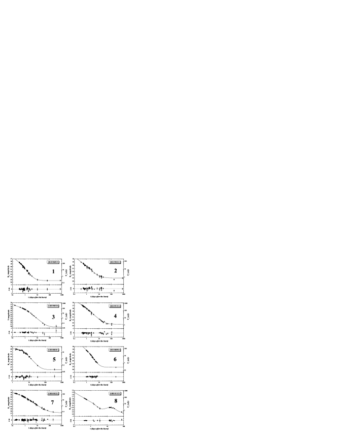
Figure 1: The light curves of the 16 afterglows we have investigated. In all but one case (GRB 990510) we have analyzed the $R_{C}$-band data. $\Delta m$ is the difference between the observed and the fitted magnitude. For GRBs 011121, 011211, and 020405 the data are corrected for the flux from the underlying host galaxy. For GRBs 030226 and 041006 the $R_{C}$-band magnitude of the host was assumed to be 27.1 and 28.4, respectively. The numbering follows Table 1.

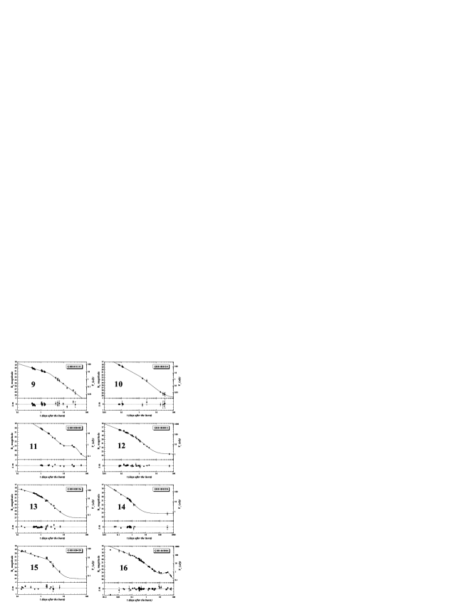
Figure 1: continued.

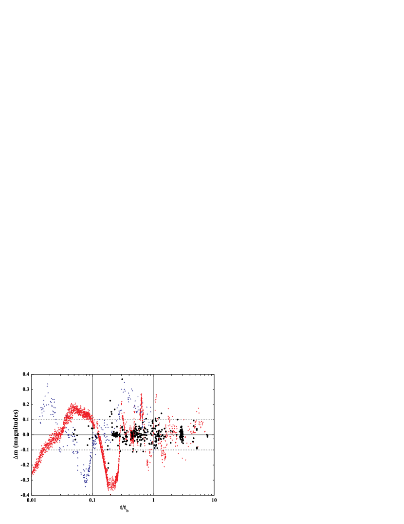
Figure 9: The residuals $\Delta m=m_{\rm observed}-m_{\rm fit}$ for all 16 afterglows in our sample (Table 1, the large black points). Included are only those data points where the reported magnitude error is less or equal than 0.05 mag. The time axis is normalized to the corresponding break time of the burst. The data indicate that any fine structure in the light curves is on average less than $\pm$0.1 magnitudes with no evidence for evolution. Note that the ratio $t/t_{b}$ is independent of redshift. For comparison, the residuals of GRB 021004 (upward pointing blue triangles) and GRB 030329 (downward pointing red triangles) are plotted. The systematic deviations from the Beuermann law are clearly seen, reaching almost 0.4 magnitudes. Furthermore, the initial fine structure of GRB 021004 and GRB 030329 is very similar; shifting the GRB 021004 light curve by a factor of 2.7 superposes this initial fine structure.

In principle, Equation (1) represents a first order approximation of an observed afterglow light curve. We consider any residuals that remain after subtraction of the fit from the observational data as the fine structure in the light curve. Since the detection of fine structure in optical afterglows depends strongly on the sampling density of the light curve and the quality of the data, an observational bias cannot be excluded, which makes it difficult to compare the fine structure among the individual afterglows. On the other hand, it is well-known that some afterglows show basically little or no evidence for fine structure when sampled very densely with the same telescope (the best example being GRB 020813; Laursen & Stanek, 2003), while others show a substantial amount of fine structure (e.g., GRB 030329; Lipkin et al., 2004, their figure 4). In order to investigate the occurrence of fine structure in more detail, we have shifted all residuals to a common evolutionary phase of an afterglow. We favor the idea that this can be done by normalizing the time $t$ that has elapsed sind the GRB trigger to the break time $t_{b}$ of the corresponding afterglow (Table 1). While Figure 1 displays the individual light curves and corresponding residuals that remain after subtraction of the fitted curves from the observational data of the 16 afterglows in our sample, Figure 9 displays all residuals in a single plot as a function of $t/t_{b}$. We have included here only those data with less or equal 0.05 mag individual photometric error. The ratio $t/t_{b}$ is independent of redshift and allows us to draw some general conclusions about the occurrence of fine structure in afterglow light curves.

First at all, again we find no evolutionary effect in the data. The width of the magnitude distribution of the fine structure of all 16 afterglows in the prebreak evolutionary era spanning one decade in time ($0.1\leq t/t_{b}\leq 1$), is identical to the width of the magnitude distribution in the postbreak era spanning one decade in time ($1\leq t/t_{b}\leq 10$), namely $\pm$ 0.1 magnitudes. The handful of data points around $t/t_{b}=0.2$ that reach beyond $\pm$0.2 magnitudes mainly belong to GRB 011211 (cf. Holland et al., 2002; Jakobsson et al., 2004a) and is statistically not significant. This picture does not change if we allow for larger individual photometric errors but then the statistical significance of this finding becomes less strong. We conclude that, on average, a patchy surface structure of afterglow shock fronts (Mészáros, Rees, & Wijers, 1998; Nakar, Piran & Granot, 2003) is not present in the photometry at times later than $t/t_{b}>0.1$, with the probable exception of GRB 011211. In addition, we find that the amplitude of the fine structure of all 16 afterglows as a group ($\pm$0.1 mag) is smaller by a factor of 4 compared to the fine structure (or fluctuations) seen in the optical afterglows of GRB 021004 (e.g., de Ugarte Postigo et al., 2005) and GRB 030329 (Lipkin et al., 2004), which are plotted in comparison. In other words, the latter two optical afterglows are indeed very different from all other afterglows we have investigated, as the deviations persist even after the break.

On the other hand, the residuals of the early afterglows of GRB 021004 and GRB 030329 are very similar. We find via $\chi^{2}$ minimization that a shift of the GRB 021004 light curve in $t/t_{b}$ by a factor of about 2.7 superposes the early light curve evolution of both bursts (the $\chi^{2}$ minimum we find is not sharp, shifts between 2.4 and 3.0 are acceptable). This is astounding, as the bursts happened at two very different cosmological epochs. A deeper analysis of this result will be pursued in a future publication (Kann et al. 2005, in preparation).

5 Summary

Based on a systematic analysis of the optical and NIR data of all GRB afterglows with sufficient published data in the pre-Swift era we have explored the parameter space of the afterglow light curves and of physical quantities related to them. From the 59 afterglows investigated (Table 1) we constructed a sample of 16 bursts with the best-defined light curves useful for our purposes. Thereby we excluded the afterglows of GRB 021004 and GRB 030329 because of their many re-brightening episodes which made it difficult to fit them.

Using the sample of the 16 afterglows with the best defined light curves, we find that in the optical bands, the average afterglow light curve is characterized by a prebreak decay slope $\alpha_{1}=1.0\pm 0.1$ and a postbreak decay slope $\alpha_{2}=2.1\pm 0.1$. The distribution of both parameters is rather broad but possible cutoffs are apparent in the available data set. In particular, there is no evidence for a universality of $\alpha_{2}$ as it has been predicted in some afterglow models. The distribution of the break time in the host frame rises sharply towards smaller values, with the most likely value at $t_{b}/(1+z)=0.3\pm 0.2$ days.

We have then used the deduced light curve parameters to extract information about the nature of the GRB environment using standard afterglow models (Panaitescu & Kumar, 2001a). We find that in most if not all cases the data are in agreement with a wind model. A general preference of an ISM model is ruled out. In addition, we find that the distribution of the power-law index $p$ of the electron distribution function is rather broad ranging from about 1.5 to 3, supporting the view of a non-universality of $p$, in agreement with other studies (e.g., Panaitescu & Kumar, 2001a, b, 2002; Preece et al., 2002; Yost et al., 2003; Panaitescu, 2005b, Paper III). Furthermore, we have searched in our data set for potential correlations between the various light curve parameters and those that characterize the corresponding burst in the gamma-ray band. With the exception of the Ghirlanda relation between the beaming corrected energy release in the gamma-ray band and peak energy in the GRB host frame (Ghirlanda et al. 2004), no other tight correlation has been found. An intriguing correlation may exist between the pre-break decay slope $\alpha_{1}$ and the smoothness parameter of the break $n$, but more data is needed to verify this.

Finally we have analyzed in which manner the data indicate to a general fine structure that is superimposed a light curve decay according to the empirical Beuermann double power-law. When normalized to the corresponding break time $t_{b}$ of a burst we find no evidence in the data that there is more structure in the light curves at times $0.1<t/t_{b}<1$ than at times $1<t/t_{b}<10$. On the other hand, we find that the afterglows of GRB 021004 and GRB 030329 are very different from all 16 afterglows in our sample. While the latter vary on average by only 0.1 magnitudes around the fitted light curve, the former vary by 0.4 magnitudes. Moreover, the fine structure of the light curves of GRB 021004 and GRB 030329 are initially very similar.

It is clear that more afterglows with well-sampled optical light curves are needed in order to get better insight onto the parameter space of the physical processes involved. Even in the Swift era this might not be an easy task since most afterglows are simply very faint some days after the burst. The observational challenge therefore remains the availability of observing time on large optical telescopes in order to determine the light curve parameters as well as possible.

Appendix A Notes on individual bursts

GRB 970508

The afterglow light curve of this GRB is anomalous, featuring an early plateau phase enduring until one day after, followed by a steep ($\alpha\approx-3.4$) re-brightening. Starting at 1.9 days, the afterglow decays with a simple power law. Our fit starts at this point. The light curve is well sampled and no break is seen, thus it is possible that the decay is postbreak (the break being hidden by the early anomalous behavior).

GRB 970815, GRB 030131

In each case, the afterglow light curve has only two data points, and a late upper limit indicates a faint host. As the degree of freedom is zero, no errors are given.

GRB 980326

The light curve fit includes a supernova component with $k=1$, $s=1$ fixed (equation 1), assuming a redshift of $z=1$ (Bloom et al., 1999).

GRB 980519

The first data point of the $R_{C}$ band light curve of the afterglow of GRB 980519 is at $t\approx 0.5$ days after the burst. In the $I_{C}$ band and $V$ band earlier data points exist but no late-time data. In order to improve the fit, we assumed achromacy and mixed these bands by shifting the $I_{C}$ and $V$ band to the same zero point as the $R_{C}$ band, fitting the composite light curve. For $t_{b}/(1+z)$, we assumed a redshift of $z=1.5$, since Jaunsen et al. (2001) state that $z\geq 1.5$ from the absence of a supernova bump in the light curve. Using $z=1.5$ also gives a very good SED fit (Paper III).

GRB 990123 and GRB 021211

These afterglow light curves have very early detections, where the light curve is dominated by reverse shock emission. Data from the reverse shock dominated phase have not been included in the fits. For GRB 021211 the result are sensitive to the data used for the fit. We used only data with $t>0.014$ days. See also our comment in § 2.

GRB 990705, GRB 020322, GRB 020410, GRB 030115, GRB 030324, GRB 031220, GRB 040422

In all these cases, afterglow data are too sparse to confine certain parameters of the light curves. The addition of observational upper limits was however used in order to derive upper or lower limits on these parameters. For light curve decay slopes, the sequence data point - upper limit - host magnitude sets a lower limit on the decay rate (e.g., GRB 020410) as the observational upper limit does not preclude an even steeper decay rate. On the other hand, the sequence upper limit - data point - host magnitude sets an upper limit on the decay rate (e.g., GRB 030324), as the upper limit cannot preclude a slower decay rate. In the case of GRB 040422, early unfiltered upper limits were, after correction for Galactic extinction, brightened by three magnitudes (the approximate typical $R_{C}-K$ color) to get early $K$-band upper limits. In some cases early data was adequate to derive $\alpha_{1}$ and a later upper limit lies beneath the extrapolated light curve decay, indicating a break in the light curve must have occurred.

GRB 991208, GRB 000131, GRB 001007

In all three cases, the optical afterglows were located several days after the burst and exhibited a steep decay $\alpha\hbox{ \raisebox{-2.84526pt}{$\stackrel{{\scriptstyle>}}{{\sim}}$} }2$. It is highly probable that the first observations are after the jet break, meaning that the decay slope is $\alpha_{2}$. For GRB 991208, the upper limit on $\alpha_{1}$ stems from a very shallow but very early upper limit (Castro-Tirado et al., 2001). We note that a postbreak decay slope is also possible for GRB 000911 (Masetti et al., 2005) – if so, it would be quite shallow. There are also several GRBs (e.g., GRB 990308, GRB 001011) where data quality is so sparse that no evidence for or against a break in the afterglow light curve can be found.

GRB 011121, GRB 020405

These bursts have relatively bright or structured hosts, which makes it difficult to extract the afterglow light curve. Different groups used different methods to do this. Therefore we decided not to mix the late data points (where the different host galaxy subtraction methods lead to significantly different magnitudes), but instead to use the data set from only one group in each case. The late data set of GRB 011121 is extracted from Greiner et al. (2003), the data set from GRB 020405 is provided by N. Masetti (private communication).

GRB 020305, GRB 030725

The late-time rebrightenings of these afterglow light curves, which have been attributed to possible supernova components (Gorosabel et al., 2005a; Pugliese et al., 2005), have not been included in the fit as no reliable redshift estimate is known. In the case of GRB 030725, there is a large data gap from 0.5 to 4.5 days. A fit that leaves $t_{b}$ as a free parameter is not confined in $\alpha_{1}$ and $t_{b}$, thus, $t_{b}$ was fixed at a reasonable value.

GRB 021004, GRB 030329

The light curves of these afterglows are clear outliers compared to the rest of our sample and very complicated to fit. The light curves each show several re-brightening episodes, which cannot be fit correctly with a smoothly broken power-law. As especially the light curve of the afterglow of GRB 030329 has been analyzed in detail (e.g., Lipkin et al., 2004), we did not do this again. As with the other afterglows, we fit smoothly broken power-laws to the light curves (the results are given in Table 1). In the case of GRB 021004, the anomalous behavior at $t<0.07$ days is excluded from the fit. We performed these fits for completeness, even though the $\chi^{2}_{\rm d.o.f.}$ values ($\chi^{2}_{\rm d.o.f.}>20$ for both) show that they are not well approximated by equation (1). While $\alpha_{1}$ is almost unaffected, $\alpha_{2}$ and $t_{b}$ are highly dependent upon the value of the smoothness parameter $n$, which had to be fixed. These results are thus not included in our statistical analysis.

If we concentrate on certain parts of the light curve of the afterglow of GRB 030329, they can be very well fit by a smoothly broken power-law. We have performed two additional fits, one using only data up to 0.55 days, before the time of the probable jet break (e.g., Uemura et al., 2003), and thus encompassing the cooling break (Sato et al., 2003), the other one using data from 0.28 days up to 1 day after the burst (the beginning of the first rebrightening) and thus encompassing the supposed jet break. In the former case, $n$ is not confined, the fit formally finds $n=450\pm 2800$, but a very sharp transition is indicated, and thus we fix $n=100$. In the last case, we were able to let the smoothness parameter $n$ vary and obtain $n=7.54\pm 1.47$ for the jet break. The values we derive for the jet break, $\alpha_{1}=1.17\pm 0.01$ and $\alpha_{2}=2.21\pm 0.07$, are both unremarkable and lie well within the distribution we find for the 16 afterglows we study here (cf. Figure 2). The slope change $\Delta\alpha$ is $\Delta\alpha=0.33\pm 0.01$ for the cooling break (slightly higher than the theoretical prediction of $\Delta\alpha=0.25$, Panaitescu & Kumar, 2001a) and $\Delta\alpha=1.04\pm 0.10$ for the jet break. This value is also unremarkable (cf. Figure 3). The rest frame break time is $0.58\pm 0.01$ days after the burst, once again typical for our sample of 16 afterglows (cf. Figure 4). The values of $\alpha_{1}$ and $\alpha_{2}$ lie very well on the theoretical line describing a Wind/ISM model with $\nu>\nu_{c}$. It is one of only a few bursts that are found in this region (cf. $\S$ 4.1, Figure 5). As the cooling frequency has passed the optical bands before the jet break and now lies at longer wavelengths, this implies an evolution from high to low frequencies and thus a wind model (Chevalier & Li, 2000).

GRB 030323

The afterglow of this GRB has a late break which is only represented by one data point. $\alpha_{2}$ was fixed to a value derived from a free fit to derive meaningful errors on $\alpha_{1}$ and $t_{b}$.

XRF 030723

The early light curve of this afterglow has a plateau phase. We do not fit this plateau phase but start at 0.9 days after the burst. While a light curve break is evident, the prebreak data are inadequate to give more than limits. We also do not fit the late time data points ($t>8$ days), which show a significant rebrightening (Fynbo et al., 2004) which can be modelled with a SN light curve only when it rises much steeper than SN1998bw. Another explanation could be that this rebrightening is caused by a two component jet (Huang et al., 2004).

GRB 040827

The steep decay of this light curve ($\alpha\geq 2$) indicates that this is a postbreak decay, but the data quality is low and the error large enough to make this conclusion unsure.

GRB 040924

The light curve is fit with an unbroken power-law, excluding the earliest data point (Fox, 2005) from the fit.

GRB 041006

As the photometric calibration of the very earliest data point of the optical afterglow (Maeno et al., 2004) is unsure, it is not included in the fit. Including it would strongly reduce $\alpha_{1}$ and $n$.

Appendix B References of host magnitudes

The following magnitudes have not been corrected for Galactic extinction and thus differ from those displayed in Table 1.

• GRB 990308: $R_{C}=29.4\pm 0.4$ mag, Jaunsen et al. (2003)

• GRB 001011: $R_{C}=25.38\pm 0.25$ mag, Gorosabel et al. (2002)

• GRB 020305: $R_{C}=25.17\pm 0.14$ mag, Gorosabel et al. (2005a)

• GRB 021004: $R_{C}=24.21\pm 0.04$ mag, de Ugarte Postigo et al. (2005)

• GRB 030115: $R_{C}=25.2\pm 0.3$ mag, Dullighan et al. (2004)

• GRB 030324: $R_{C}=25.16\pm 0.24$ mag, Nysewander et al. (2004)

• GRB 030329: $R_{C}=22.66\pm 0.04$ mag, Gorosabel et al. (2005b)

Table 1: Results of the light curve fitting (Equation 1)

GRB	#	band	$\chi^{2}_{dof}$	$d.o.f.$	$m_{c}$	$\alpha_{1}$	$\alpha_{2}$	$t_{b}$	$n$	$m_{\rm host}$
970228		$R_{C}$	0.70	4	20.43$\pm$0.21	1.46$\pm$0.15	$\cdots$	$\cdots$	$\cdots$	24.65$\pm$0.51
970508		$R_{C}$	3.95	61	18.64$\pm$0.02	1.24$\pm$0.01	$\cdots$	$\cdots$	$\cdots$	25.29$\pm$0.09
970815		$I_{C}$	$\cdots$	0	21.73	0.34	$\cdots$	$\cdots$	$\cdots$	25
971214		$R_{C}$	1.12	10	22.91$\pm$0.05	1.49$\pm$0.08	$\cdots$	$\cdots$	$\cdots$	25.64$\pm$0.05
980326		$R_{C}$	2.74	16	22.82$\pm$0.04	1.85$\pm$0.05	$\cdots$	$\cdots$	$\cdots$	28.95$\pm$0.53
980329		$R_{C}$	2.85	8	23.91$\pm$0.17	0.85$\pm$0.12	$\cdots$	$\cdots$	$\cdots$	26.67$\pm$0.10
980519	1	$R_{C}$	2.73	68	18.86$\pm$0.13	1.50$\pm$0.12	2.27$\pm$0.03	0.48$\pm$0.03	10	25.36$\pm$0.12
980613		$R_{C}$	$<0.01$	1	23.07$\pm$0.21	0.44$\pm$0.23	$\cdots$	$\cdots$	$\cdots$	24.04$\pm$0.50
980703		$R_{C}$	0.77	13	21.51$\pm$0.96	0.85$\pm$0.84	1.65$\pm$0.46	1.35$\pm$0.94	10	22.46$\pm$0.08
990123	2	$R_{C}$	2.11	44	21.37$\pm$0.60	1.24$\pm$0.06	1.62$\pm$0.15	2.06$\pm$0.83	10	23.99$\pm$0.09
990308		$R_{C}$	$<0.01$	1	22.28$\pm$4.00	$\cdots$	1.96$\pm$1.89	$\cdots$	$\cdots$	29.34
990510	3	$V$	1.57	59	19.50$\pm$0.05	0.92$\pm$0.02	2.10$\pm$0.06	1.31$\pm$0.07	2.25$\pm$0.51	28.37$\pm$0.48
990705		$H$	$\cdots$	$\cdots$	$\geq 18.3$	$\leq 1.68$	$\geq 2.88$	$\geq 0.75$	10	22
990712		$R_{C}$	1.27	18	21.22$\pm$0.02	0.96$\pm$0.02	$\cdots$	$\cdots$	$\cdots$	21.80$\pm$0.02
991208		$R_{C}$	1.74	12	16.60$\pm$0.07	$\leq 1.38$	2.47$\pm$0.05	$\leq 2.08$	$\cdots$	24.28$\pm$0.16
991216	4	$R_{C}$	1.47	65	18.09$\pm$0.18	1.17$\pm$0.03	1.57$\pm$0.03	1.10$\pm$0.13	10	23.52$\pm$0.09
000131		$R_{C}$	0.18	1	19.88$\pm$0.31	$\cdots$	2.40$\pm$0.21	$\cdots$	$\cdots$	27
000301	5	$R_{C}$	4.93	50	20.70$\pm$0.06	0.57$\pm$0.05	2.81$\pm$0.13	4.93$\pm$0.18	2.36$\pm$0.67	27.95$\pm$0.30
000418		$R_{C}$	1.68	16	23.18$\pm$0.94	1.15$\pm$0.41	2.69$\pm$0.66	7.85$\pm$2.71	10	23.46$\pm$0.03
000630		$R_{C}$	0.46	5	23.19$\pm$0.06	1.12$\pm$0.11	$\cdots$	$\cdots$	$\cdots$	26.68$\pm$0.21
000911		$R_{C}$	0.34	8	19.67$\pm$0.09	1.46$\pm$0.04	$\cdots$	$\cdots$	$\cdots$	25.11$\pm$0.11
000926	6	$R_{C}$	1.10	49	20.81$\pm$0.16	1.74$\pm$0.03	2.45$\pm$0.05	2.10$\pm$0.15	10	25.22$\pm$0.06
001007		$R_{C}$	0.52	4	17.48$\pm$0.22	$\cdots$	2.06$\pm$0.13	$\cdots$	$\cdots$	24.73$\pm$0.15
001011		$R_{C}$	$<0.01$	1	22.45$\pm$0.16	1.45$\pm$0.14	$\cdots$	$\cdots$	$\cdots$	25.19
010222	7	$R_{C}$	2.05	133	19.21$\pm$0.24	0.60$\pm$0.09	1.44$\pm$0.02	0.64$\pm$0.09	2.29$\pm$0.68	26.68$\pm$0.17
010921		$r^{\prime}$	0.97	4	19.46$\pm$0.03	1.56$\pm$0.07	$\cdots$	$\cdots$	$\cdots$	21.63$\pm$0.02
011121	8	$R_{C}$	1.27	17	20.27$\pm$0.32	1.76$\pm$0.05	2.99$\pm$0.28	1.54$\pm$0.22	10	host corrected
011211	9	$R_{C}$	7.21	43	21.72$\pm$0.15	0.93$\pm$0.02	2.31$\pm$0.27	2.34$\pm$0.34	10	host corrected
020124	10	$R_{C}$	0.71	10	22.85$\pm$1.00	1.47$\pm$0.06	2.12$\pm$0.27	1.36$\pm$0.77	10	30.68$\pm$2.28
020305		$R_{C}$	3.38	4	19.60$\pm$0.20	1.19$\pm$0.07	$\cdots$	$\cdots$	$\cdots$	25.04
020322		$R_{C}$	$<0.01$	1	23.66$\pm$0.49	0.45$\pm$0.39	$\geq$2.17	0.95$\pm$0.27	10	host corrected
020331		$R_{C}$	1.98	6	22.56$\pm$0.26	0.69$\pm$0.04	2.12$\pm$0.40	7.17$\pm$1.52	10	24.89$\pm$0.16
020405	11	$R_{C}$	5.26	12	21.35$\pm$0.32	1.26$\pm$0.09	1.93$\pm$0.13	2.40$\pm$0.45	10	host corrected
020410		$R_{C}$	$\cdots$	$\cdots$	$\leq 22.4$	$\geq 1.25$	$\cdots$	$\cdots$	$\cdots$	28.23$\pm$0.5
020813	12	$R_{C}$	2.00	59	19.27$\pm$0.11	0.67$\pm$0.07	1.78$\pm$0.28	0.77$\pm$0.25	1.44$\pm$1.06	23.61$\pm$0.15
020903		$R_{C}$	1.52	3	19.54$\pm$0.21	1.27$\pm$0.58	$\cdots$	$\cdots$	$\cdots$	20.91$\pm$0.47
021004		$R_{C}$	38.5	378	21.62$\pm$0.02	1.07$\pm$0.01	2.12$\pm$0.07	8.62$\pm$0.16	10	24.06
021211		$R_{C}$	2.00	27	20.30$\pm$0.90	0.96$\pm$0.04	1.22$\pm$0.10	0.11$\pm$0.09	10	25.20$\pm$0.12
030115		$R_{C}$	0.10	1	$\geq 20.30$	0.44$\pm$0.12	$\geq 3$	$\geq 2$	10	24.8
030131		$R_{C}$	$\cdots$	0	23.35	1.06	$\cdots$	$\cdots$	$\cdots$	30
030226	13	$R_{C}$	3.86	35	19.67$\pm$0.33	0.58$\pm$0.16	2.68$\pm$0.28	0.96$\pm$0.10	0.91$\pm$0.49	27.1
030227		$R_{C}$	1.07	4	22.83$\pm$0.11	1.18$\pm$0.15	$\cdots$	$\cdots$	$\cdots$	25
030323		$R_{C}$	2.16	36	22.94$\pm$0.18	1.36$\pm$0.02	2.7	6.71$\pm$0.74	10	27.86$\pm$0.52
030324		$I_{C}$	$\cdots$	$\cdots$	$\leq 25.65$	$\leq 1.32$	$\cdots$	$\cdots$	$\cdots$	25
030328	14	$R_{C}$	1.34	18	20.61$\pm$0.23	0.87$\pm$0.04	1.54$\pm$0.11	0.60$\pm$0.10	10	24.15$\pm$0.35
030329		$R_{C}$	30.4	2953	17.63$\pm$0.01	1.10$\pm$0.01	2.32$\pm$0.01	5.27$\pm$0.02	10	22.60
030329		$R_{C}$	0.85	1165	13.92$\pm$0.01	0.86$\pm$0.01	1.19$\pm$0.01	0.27$\pm$0.01	100	22.60
030329		$R_{C}$	0.64	946	15.11$\pm$0.03	1.17$\pm$0.01	2.21$\pm$0.07	0.68$\pm$0.02	7.54$\pm$1.47	22.60
030418		$R_{C}$	0.42	10	22.22$\pm$1.31	1.23$\pm$0.09	1.72$\pm$0.48	1.50$\pm$1.26	10	27
030429	15	$R_{C}$	7.68	11	21.80$\pm$0.08	0.81$\pm$0.03	3.03$\pm$0.27	2.17$\pm$0.09	10	27
030528		$Ks$	0.53	1	19.28$\pm$0.65	0.73$\pm$0.89	$\cdots$	$\cdots$	$\cdots$	19.82$\pm$0.75
030723		$R_{C}$	1.61	12	$\leq 21.45$	$\leq 0.88$	2.12$\pm$0.06	$\leq 1.57$	10	27
030725		$R_{C}$	1.31	8	20.45$\pm$0.05	0.80$\pm$0.06	1.65$\pm$0.06	2.9	10	25
031203		$J$	0.20	24	19.36$\pm$0.98	0.69$\pm$0.50	$\cdots$	$\cdots$	$\cdots$	17.43$\pm$0.15
031220		$R_{C}$	$\cdots$	$\cdots$	$\leq 23.7$	$\leq 1.77$	$\cdots$	$\cdots$	$\cdots$	23.13$\pm$0.11
040106		$R_{C}$	0.05	1	22.86$\pm$0.10	1.31$\pm$0.11	$\cdots$	$\cdots$	$\cdots$	28
040422		$Ks$	$\cdots$	$\cdots$	$\leq 21.28$	$\leq 1.3$	$\cdots$	$\cdots$	$\cdots$	19.74$\pm$0.17
040827		$Ks$	1.52	11	21.05$\pm$0.34	$\cdots$	2.08$\pm$0.45	$\cdots$	$\cdots$	20.00$\pm$0.05
040916		$R_{C}$	0.59	3	23.64$\pm$0.11	0.96$\pm$0.07	$\cdots$	$\cdots$	$\cdots$	30
040924		$R_{C}$	1.37	29	22.96$\pm$0.04	1.09$\pm$0.02	$\cdots$	$\cdots$	$\cdots$	24.55$\pm$0.19
041006	16	$R_{C}$	1.25	81	19.45$\pm$0.27	0.68$\pm$0.06	1.30$\pm$0.02	0.23$\pm$0.04	4.87$\pm$2.57	28.4

Table 2: The absolute value of the correlation coefficient between the various parameters

	$\Delta\alpha$	$t_{b}/(1+z)$	$\theta_{\rm jet,ISM}$	$\theta_{\rm jet,wind}$	$\theta_{\rm jet,mixed}$	$\log(E_{\rm cor,ISM})$	$\log(E_{\rm cor,wind})$	$\log(E_{\rm cor,mixed})$	$\log(E_{\rm peak})$	$z$
$\alpha_{1}$	0.50	0.30	0.55	0.33	0.02	0.29	0.39	0.37	0.46	0.20
$\alpha_{2}$	0.65	0.46	0.69	0.74	0.66	0.49	0.51	0.50	0.77	0.75
$\Delta\alpha$	$\cdots$	0.62	0.36	0.55	0.37	0.40	0.19	0.24	0.31	0.55
$t_{b}/(1+z)$	$\cdots$	$\cdots$	0.82	0.58	0.62	0.28	0.31	0.29	0.01	0.53
$\theta_{\rm jet,ISM}$	$\cdots$	$\cdots$	$\cdots$	$\cdots$	$\cdots$	0.14	0.37	0.28	0.18	0.00
$\theta_{\rm jet,wind}$	$\cdots$	$\cdots$	$\cdots$	$\cdots$	$\cdots$	0.49	0.66	0.67	0.53	0.14
$\theta_{\rm jet,mixed}$	$\cdots$	$\cdots$	$\cdots$	$\cdots$	$\cdots$	0.43	0.58	0.52	0.55	0.15
$\log(E_{\rm cor,ISM})$	$\cdots$	$\cdots$	$\cdots$	$\cdots$	$\cdots$	$\cdots$	$\cdots$	$\cdots$	0.81	0.05
$\log(E_{\rm cor,wind})$	$\cdots$	$\cdots$	$\cdots$	$\cdots$	$\cdots$	$\cdots$	$\cdots$	$\cdots$	0.91	0.03
$\log(E_{\rm cor,mixed})$	$\cdots$	$\cdots$	$\cdots$	$\cdots$	$\cdots$	$\cdots$	$\cdots$	$\cdots$	0.78	0.03
$\log(E_{\rm peak})$	$\cdots$	$\cdots$	$\cdots$	$\cdots$	$\cdots$	$\cdots$	$\cdots$	$\cdots$	$\cdots$	0.01

Figure 5: The afterglow parameters $\alpha_{1}$ and $\alpha_{2}$ in comparison with standard afterglow models (Panaitescu & Kumar, 2001a). The dashed line is for an ISM density profile with $\nu<\nu_{c}$, the dotted line for the ISM/wind model with $\nu>\nu_{c}$ and a Compton parameter, $Y$, less than 1, and the solid line for the wind model with $\nu<\nu_{c}$. Note that we have extended these curves to $\alpha_{2}<2.0$. The two curves around ($\alpha_{1}=1.0,\alpha_{2}=2.0$) represent the case $\nu>\nu_{c}$, $Y>1,2<p<3$ (Panaitescu & Kumar, 2001a). The dash-dotted line stands for the theoretical prediction of the passage of the cooling break ($\alpha_{2}=\alpha_{1}+0.25$). While GRB 990123 (# 2) lies on this line within errors, it has a late achromatic break which is very probably a shallow jet break.

Figure 7: The Ghirlanda relation (Ghirlanda et al. 2004) as it follows from our light curve data (Table 1, § 4.2) in combination with the high-energy data given in Friedman & Bloom (2005). GRB #1 is not shown because of the uncertainty of its redshift and GRBs #5, #6, #7 are not included here since $E_{\rm peak}$ is not known. Our fit gives a slope of $0.79\pm 0.09$ if the outliers GRB 011211 (# 9) and 020813 (# 12) are excluded. For comparison, the dotted line shows the relation obtained by Ghirlanda et al. (2004) based on their data base.

Figure 8: The relation between the prebreak decay slope $\alpha_{1}$ and the smoothness of the break $n$ (Equation 1). For all afterglows not in this figure we had to fix the smoothness parameter to a relatively high value of $n=10$ to get an acceptable fit (Table 1). All these fits also find $\alpha_{1}>1$. In addition, we include here a special fit of the afterglow of GRB 030329 as explained in the text (§ 4.3 and Appendix A). This is the only fit where $\alpha_{1}>1$ and a value for $n$ could be deduced.

References

- Achterberg et al. (2001) Achterberg, A., Gallant, Y. A., Kirk, J. G., & Guthmann, A. W. 2001, MNRAS, 328, 393
- Amati et al. (2002) Amati, L., et al. 2002, A&A, 390, 81
- Band & Preece (2005) Band, D. L., & Preece, R. D. 2005, ApJ, 627, 319
- Beuermann et al. (1999) Beuermann, K., et al. 1999, A&A, 352, L26
- Bhattacharya (2001) Bhattacharya, D. 2001, Bull. Astron. Soc. India, 29, 107
- Bloom et al. (1999) Bloom, J. S., et al. 1999, Nature, 401, 453
- Bloom, Frail & Kulkarni (2003) Bloom, J. S., Frail, D. A., & Kulkarni, S. R. 2003, ApJ, 594, 674
- Castro-Tirado et al. (2001) Castro-Tirado, A. J., et al. 2001, A&A, 370, 398
- Chevalier & Li (2000) Chevalier, R. A. & Li, Z. 2000, ApJ, 536, 195
- Dai & Cheng (2001) Dai, Z. G., & Cheng, K. S. 2001, ApJ, 558, L109
- Dai, Liang & Xu (2004) Dai, Z. G., Liang, E. W., & Xu, D. 2004, ApJ, 612, L101
- de Ugarte Postigo et al. (2005) de Ugarte Postigo, A., et al. 2005, A&A, in press (astro-ph/0506544)
- Dullighan et al. (2004) Dullighan, A., Ricker, G., Butler, N., & Vanderspek, R., in: Gamma-Ray Bursts: 30 Years of Discovery: Gamma-Ray Burst Symposium. AIP Conf. Proc. 727, 467 (astro-ph/0401062)
- Fox et al. (2003) Fox, D. W., et al. 2003, ApJ, 586, L5
- Fox (2005) Fox, D. B. 2005, GCN 2741
- Frail et al. (2001) Frail, D. A., et al. 2001, ApJ, 562, L55
- Frail et al. (2003a) Frail, D. A. et al. 2003a, AJ, 125, 2299
- Frail et al. (2003b) Frail, D. A. et al. 2003b, ApJ, 590, 992
- Frail et al. (2004) Frail, D. A., Metzger, B. D., Berger, E., Kulkarni, S. R., & Yost, S. A. 2004, ApJ, 600, 828
- Freedman & Waxman (2001) Freedman, D. L., & Waxman, E. 2001, ApJ, 547, 922
- Friedman & Bloom (2005) Friedman, A. S., & Bloom, J. S. 2005, ApJ, 627, 1
- Frontera et al. (2000) Frontera, F., et al. 2000, ApJS, 127, 59
- Fynbo et al. (2004) Fynbo, J. P. U., et al. 2004, ApJ, 609, 962
- Garnavich, Loeb, & Stanek (2000) Garnavich, P. M., Loeb, A., & Stanek, K. Z. 2000, ApJ, 544, L11
- Gaudi, Granot & Loeb (2001) Gaudi, B. S., Granot, J., & Loeb, A. 2001, ApJ, 561, 178
- Gehrels (2004) Gehrels, N. 2004, New Astron. Reviews, 48, 431
- Gendre & Boër (2005) Gendre, B., & Boër, M. 2005, A&A, 430, 465
- Ghirlanda, Ghisellini & Lazzati (2004) Ghirlanda, G., Ghisellini, G., & Lazzati, D. 2004, ApJ, 616, 331
- Gorosabel et al. (2002) Gorosabel, J., et al. 2002, A&A, 384, 11
- Gorosabel et al. (2005a) Gorosabel, J., et al. 2005a, A&A, 437, 411
- Gorosabel et al. (2005b) Gorosabel, J., et al. 2005b, A&A, in press (astro-ph/0507488)
- Greiner et al. (2003) Greiner, J., et al. 2003, ApJ, 599, 1223
- Groot et al. (1997) Groot, P. J., et al. 1997, IAU Circ. 6584
- Holland et al. (2002) Holland, S. T., et al. 2002, AJ, 124, 639
- Holland et al. (2004) Holland, S. T., et al. 2004, AJ, 128, 1955
- Huang et al. (2004) Huang, Y. F., Wu, X. F., Dai, Z. G., Ma, H. T., & Lu, T. 2004, ApJ, 605, 300
- Jakobsson et al. (2004a) Jakobsson, P., et al. 2004, New Astron., 9, 435
- Jakobsson et al. (2004b) Jakobsson, P., et al. 2004, A&A, 427, 785
- Jaunsen et al. (2001) Jaunsen, A. O., et al. 2001, ApJ, 546, 127
- Jaunsen et al. (2003) Jaunsen, A. O., et al. 2003, A&A, 402, 125
- Kann, Klose, & Zeh (2005) Kann, D. A., Klose, S., & Zeh, A. 2005, ApJ, submitted (Paper III)
- Kirk et al. (2000) Kirk, J. G., Guthmann, A. W., Gallant, Y. A., & Achterberg, A. 2000, ApJ, 542, 235
- Klose et al. (2004) Klose, S., et al. 2004, AJ, 128, 1942
- Kumar & Panaitescu (2003) Kumar, P. & Panaitescu, A. 2003, MNRAS, 346, 905
- Laursen & Stanek (2003) Laursen, L. T., & Stanek, K. Z. 2003, ApJ, 597, L107
- Li et al. (2003) Li, W., et al. 2003, ApJ, 586, L9
- Liang (2004) Liang, E. W. 2004, MNRAS, 348, 153
- Lipkin et al. (2004) Lipkin, Y. M., et al. 2004, ApJ, 606, 381
- Livio & Waxman (2000) Livio, M., & Waxman, E. 2000, ApJ, 538, 187
- MacFadyen, Woosley, & Heger (2001) MacFadyen, A. I., Woosley, S. E., & Heger, A. 2001, ApJ, 550, 410
- Maeno et al. (2004) Maeno, S., et al. 2004, GCN 2772
- Masetti et al. (2005) Masetti, N., et al. 2005, A&A, 438, 841
- Mészáros, Rees, & Wijers (1998) Mészáros, P., Rees, M. J., & Wijers, R. A. M. J. 1998, ApJ, 499, 301
- Nakar, Piran & Granot (2003) Nakar, E., & Piran, T., & Granot, J. 2003, New Astron., 8, 495
- Nakar & Piran (2005) Nakar, E., & Piran, T. 2005, MNRAS, 360, L73
- Nysewander et al. (2004) Nysewander, M. C., Price, P. A., Reichart, D. E., & Lamb, D. Q. 2004, GCN 2601
- Nysewander et al. (2005) Nysewander, M. C., et al. 2005, ApJ, submitted (astro-ph/0505474)
- Panaitescu & Kumar (2001a) Panaitescu, A., & Kumar, P. 2001a, ApJ, 554, 667
- Panaitescu & Kumar (2001b) Panaitescu, A., & Kumar, P. 2001b, ApJ, 560, L49
- Panaitescu & Kumar (2002) Panaitescu, A., & Kumar, P. 2002, ApJ, 571, 779
- Panaitescu (2005a) Panaitescu, A. 2005a, MNRAS, 362, 921
- Panaitescu (2005b) Panaitescu, A. 2005b, MNRAS, in press (astro-ph/0508426)
- Piran (2005) Piran, T. 2005, Rev. Mod. Phys., 76, 1143
- Preece et al. (2002) Preece, R. D., et al. 2002, ApJ, 581, 1248
- Pugliese et al. (2005) Pugliese, G., et al. 2005, A&A, 439, 527
- Rhoads (1999) Rhoads, J. E. 1999, ApJ, 525, 737
- Sakamoto et al. (2005) Sakamoto, T., et al. 2005, ApJ, 629, 311
- Sari, Piran, & Halpern (1999) Sari, R., Piran, T., & Halpern, J. P. 1999, ApJ, 519, L17
- Sato et al. (2003) Sato, R., et al. 2003, ApJ, 599, L9
- Schlegel, Finkbeiner, & Davis (1998) Schlegel, D. J., Finkbeiner, D. P., & Davis, M. 1998, ApJ, 500, 525
- Stratta et al. (2004) Stratta, G., et al. 2004, ApJ, 608, 846
- Uemura et al. (2003) Uemura, M., et al. 2003, Nature, 423, 843
- van Paradijs et al. (1997) van Paradijs, J., et al. 1997, Nature, 386, 686
- Wei (2003) Wei, D. M. 2003, A&A, 402, L9
- Wu et al. (2004) Wu, X. F., Dai, Z. G., & Liang, E. W. 2004, ApJ, 615, 359
- Yost et al. (2002) Yost, S. A., et al. 2002, ApJ, 577, 155
- Yost et al. (2003) Yost, S. A., Harrison, F. A., Sari, R., & Frail, D. A. 2003, ApJ, 597, 459
- Zeh, Klose, & Hartmann (2004) Zeh, A., Klose, S., & Hartmann, D. H. 2004, ApJ, 609, 952 (Paper I)
- Zeh, Klose, & Hartmann (2005) Zeh, A., Klose, S., & Hartmann, D. H. 2005, Proc. 22nd Texas Symp. Relativistic Astrophysics, astro-ph/0503311
- Zhang & Mészáros (2004) Zhang, B., & Mészáros, P. 2004, Int. J. Mod. Phys., A19, 2385