Supernova Constraints on Models of Neutrino Dark Energy

Abstract

In this paper we use the recently released Type Ia Supernova (SNIa) data to constrain the interactions between the neutrinos and the dark energy scalar fields. In the analysis we take the dark energy scalars to be either Quintessence-like or Phantom-like. Our results show the data mildly favor a model where the neutrinos couple to a phantom-like dark energy scalar, which implies the equation of state of the coupled system behaves like Quintom scenario in the sense of parameter degeneracy. We find future observations like SNAP are potentially promising to measure the couplings between neutrino and dark energy.

PACS number(s): 98.80.Es

I Introduction

Astronomical observations of the Type Ia Supernova (SNIa), Cosmic Microwave Background Radiation(CMB) and the Large Scale Structure(LSS) strongly support for a concordance model of cosmology where the universe is flat and composed of around seventy percent of dark energy(DE)[1, 2, 3]. The simplest candidate for dark energy seems to be a remnant small cosmological constant. However, many physicists are attracted by the idea that dark energy is due to a dynamical component, such as a canonical scalar field $Q$, named Quintessence[4]. The recent fits to the SNIa data and CMB etc in the literature find that the behavior of dark energy is to great extent in consistency with a cosmological constant, however the dynamical dark energy scenarios are generally not ruled out and in fact one class of models with an equation of state(EOS) transiting from below -1 to above -1 as the redshift increases, Quintom[5, 6] is mildly favored[7]. Being a dynamical component, the scalar field of dark energy is expected to interact with the ordinary matters. If these interactions exist, it will open up the possibility of detecting the dark energy non-gravitationally.

Recently there have been a lot of interests in the literature in studying the possible connections between the neutrinos and the dark energy.[8, 9, 10, 11, 12, 13, 14, 15, 16, 17, 18, 19, 20, 21, 22, 25, 23] There seem to be at least two reasons which motivate these studies: 1) the dark energy scale $\sim 10^{-3}$ ev is smaller than the energy scales in particle physics, but interestingly is comparable to the neutrino masses; 2) in Quintessence-like models of dark energy $m_{Q}\sim 10^{-33}$ eV, which surprisingly is also connected to the neutrino masses via a see-saw formula $m_{Q}\sim{m_{\nu}^{2}/m_{pl}}$ with $m_{pl}$ the planck mass.

Is there really any connections between the neutrinos and dark energy? Given the arguments above it is quite interesting to make such a speculation on this connection. If yes, however in terms of the language of the particle physics it requires the existence of new dynamics and new interactions between the neutrinos and the dark energy sector.

In general for the models of neutrino dark energy or interacting dark energy, the lagrangian can be written as

$${\cal L}={\cal L}^{SM}_{\nu}+{\cal L}_{\phi}+{\cal L}_{int},$$ (1)

where ${\cal L}^{SM}_{\nu}$ is the lagrangian of the standard model (SM) describing the physics of the left-handed neutrinos, ${\cal L}_{\phi}$ is for the dynamical scalar such as Quintessence. ${\cal L}_{int}$ in (1) is the sector which mediates the interaction between the dark energy scalar and the neutrinos.

At energy much below the electroweak scale, the relevant lagrangian for the neutrino dark energy is given by

$${\cal L}={\cal L}_{\nu}+{\cal L}_{\phi}+M_{\nu}(\phi)\bar{\nu}{\nu}\ ,$$ (2)

where ${\cal L}_{\nu}$ is the kinetic term of the neutrinos. For the dark energy scalar part of ${\cal L}_{\phi}$, two types of models have often been considered with one being the quintessence-like and another phantom-like[24]. Thus we introduce a factor $F$ in the front of the kinetic term of the scalar

$${\cal L}_{\phi}=\frac{F}{2}\partial_{\mu}\phi\partial^{\mu}\phi-V(\phi).$$ (3)

When $F=1$ it corresponds to quintessence-like and $F=-1$ for phantom-like. $V(\phi)$ is the potential of the scalar field.

The last term of Eq.(2) is the scalar field dependent mass of the neutrinos which characterizes the interaction between the neutrinos and the dark energy scalar. In the standard model of particle physics, the neutrino masses can be described by a dimension-5 operator

$$L_{\not L}=\frac{2}{f}l_{L}l_{L}HH+h.c,$$ (4)

where $f$ is a scale of new physics beyond the Standard Model which generates the $B-L$ violations, $l_{L},H$ are the left-handed lepton and Higgs doublets respectively. When the Higgs field gets a vacuum expectation value $<H>\sim v$, the left-handed neutrino receives a majorana mass $m_{\nu}\sim\frac{v^{2}}{f}$. In Ref.[11] we considered an interaction between the neutrinos and the Quintessence $\phi$

$$\beta\frac{\phi}{M_{pl}}\frac{2}{f}l_{L}l_{L}HH+h.c,$$ (5)

where $\beta$ is the coefficient which characterizes the strength of the Quintessence interacting with the neutrinos. In this scenario the neutrino masses vary during the evolution of the universe and we have shown that the neutrino mass limits imposed by the baryogenesis are modified.

The dim-5 operator above is not renormalizable, which in principle can be generated by integrating out the heavy particles. For example, in the model of the minimal see-saw mechanism for the neutrino masses,

$$L=h_{ij}\bar{l}_{Li}N_{Rj}H+\frac{1}{2}M_{ij}\bar{N}^{c}_{Ri}N_{Rj}+h.c.$$ (6)

where $M_{ij}$ is the mass matrix of the right-handed neutrinos and the Dirac masses of the neutrinos are given by $m_{D}\equiv h_{ij}<H>$. Integrating out the heavy right-handed neutrinos one will generate a dim-5 operator, however as pointed out in Ref.[11] to have the light neutrino masses varied there are various possibilities, such as by coupling the Quintessence field to either the Dirac masses or the majorana masses of the right-handed neutrinos or both.

In Ref.[13] we have specifically proposed a model of mass varying right-handed neutrinos. In this model the right-handed neutrino masses $M_{i}$ are assumed to be a function of the Quintessence scalar $M_{i}(\phi)=\overline{M}_{i}e^{\beta\frac{\phi}{M_{pl}}}$. Integrating out the right-handed neutrino will generate a dimension-5 operator, but for this case the light neutrino masses will vary in the following way

$$e^{-\beta\frac{\phi}{M_{pl}}}\frac{2}{f}l_{L}l_{L}HH+h.c.$$ (7)

With mass varying right-handed neutrinos given above we have in [13] studied in detail its implication in thermal leptogenesis. In Ref.[21] we have studied the possibility of detecting the time variation of the neutrino masses with Short Gamma Ray Burst. In Ref. [22] we have discussed the implications of the mass varying neutrinos in the cosmological evolution of the Universe. And in Ref.[23] we argued that neutrinos coupled to Phantom scalar can provide a scenario of dark energy with the equation of state crossing the cosmological constant boundary of -1. In this paper we will use the recently released SNIa data to constrain the couplings between the neutrinos and the dark energy scalar. We will show that the current data mildly favor the model where the Phantom-like scalar couples to the neutrinos. This paper is organized as follows: in section II we will present the formulation and the results on the constraint on the equation of state of the coupled system; In section III we study the constraints on the couplings of the neutrinos to the scalar fields; Section IV is our conclusion.

II Formulation and the constraint on the equation of state

In this section we will study in detail the scenario of the coupled system of neutrino and scalar field described by the lagrangian in (2). The equation of motion of the scalar field $\phi$ is given by

$$F(\ddot{\phi}+3H\dot{\phi})+\frac{dV}{d\phi}+\frac{dV_{I}}{d\phi}=0\ ,$$ (8)

where

$$\frac{dV_{I}}{d\phi}=\frac{dM_{\nu}}{d\phi}n_{\nu}\left\langle\frac{M_{\nu}}{E}\right\rangle$$ (9)

is the source term by the interaction between the neutrinos and dark energy, with $n_{\nu}$ and $E$ being the number density and energy of the neutrinos respectively and $\langle\rangle$ indicating the thermal average. For relativistic neutrinos, the term $\frac{dV_{I}}{d\phi}$ is greatly suppressed and the neutrinos and dark energy decouple. For non-relativistic neutrinos, the effective potential of the system is given by $V_{eff}(\phi)=V(\phi)+n_{\nu}M_{\nu}(\phi)$. In the following, for the simplicity we take the $\phi$-depending neutrino mass $M_{\nu}(\phi)$ as $M_{\nu}$.

For this coupled system, the energy for each component does not conserve while the total number of neutrinos is constant. It is easy to get that the energy density of neutrinos follows

$$\dot{\rho}_{\nu}+3H\rho_{\nu}=n_{\nu}\dot{M_{\nu}}.$$ (10)

The conservation of energy-momentum tensor of the whole system gives that the fluid equation of the scalar field $\phi$ is

$$\dot{\rho}_{\phi}+3H\rho_{\phi}(1+w_{\phi})=-n_{\nu}\dot{M_{\nu}}\ ,$$ (11)

with the corresponding equation of state $w_{\phi}\equiv P_{\phi}/\rho_{\phi}=\frac{\frac{1}{2}F\dot{\phi}^{2}-V(\phi)}{\frac{1}{2}F\dot{\phi}^{2}+V(\phi)}$, which stands for the uncoupled equation of state and F has the same convention as that in Eq. (3).

From Eqs. (10) and (11) one can easily obtain the equation of state of the whole coupled system

$$w=\frac{\Omega_{\phi}}{\Omega_{\nu}+\Omega_{\phi}}w_{\phi}.$$ (12)

In the following, we will use the recently released SNIa data[1] to constrain this class of models. For the low redshift range covered by the geometric constraints of SNIa the equation of state of the coupled system can be simply parameterized as $w=w_{0}+w_{1}z$. In the left panel of Fig. 1 we plot the parameter space of $(w_{0},w_{1})$ constrained by the SNIa data. One can see the best fitting values are around $w_{0}=-1.75$ and $w_{1}=1.9$, which gives rise to an evolving EOS and transiting from below -1 to above -1 as the redshift increases as shown in the right panel of Fig.1. In our case for a constant equation of state the best fitting value corresponds to $w=-1.45$. On the current SNIa fittings we have assumed the matter energy density fraction to be in the range $0.2<\Omega_{m}<0.4$, which is somewhat optimistic. This will inevitably lead to some bias but does not affect the physical picture of this paper. On the degeneracies between $\Omega_{m}$ and dark energy EOS see e.g. [26, 5, 27, 28]. Generically one needs to add some priors or combined data analysis to extract the behaviors of dynamical dark energy[1, 7]. A thorough combined observational constraints on the couplings needs the modification of the Boltzman code and investigations on the full set of parameter space, which is extremely time-consuming in computation with the massive neutrinos (for a preliminary model-dependent study see [29]). In this paper we assume a flat prior of the Universe, i.e. $\Omega_{k}=0$.

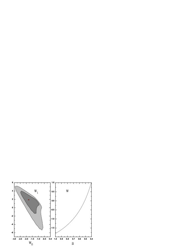
Figure 1: The left panel: 2 $\sigma$ SNIa limit on the Dark Energy model whose equation of state is $w=w_{0}+w_{1}z$ with prior $0.2<\Omega_{m}<0.4$; The right panel: the evolution of $w$ as function of scale factor $a$ with the center value given by the left panel.

From equation $(\ref{whole w})$, one can see that to have $w$ transit from below $-1$ to above $-1$ as the redshift increases we need $w_{\phi}<-1$ which implies the scalar field to be a Phantom-like. In the next section we will use the SNIa data to constrain the coupling of the neutrinos to the scalar field. We will point out that the interaction between the neutrinos and the phantom field is crucial to the Quintom scenario of dark energy.

III Constraint on the coupling of neutrinos to the scalar field

Current experiments have put somewhat stringent constraints on the conventional neutrino mass. Atmosphere neutrino oscillations show that there is at least one species of neutrino with mass $\gtrsim 0.05$ eV[31]. Measurements of LSS matter power spectrum are very sensitive to the total mass of neutrino and a combined analysis from WMAP[2] and SDSS[3] gives an upper bound $\Sigma m_{\nu}<1.7$ eV at $95\%$ C.L. A recent analysis has optimistically constrained the upper bound to be 0.42 eV. Cosmological combined constraints on $\Sigma m_{\nu}$ are faced with many parameter degeneracies and a recent interesting study[32] has shown the degeneracy between dark energy EOS and neutrino mass, which can loosen the upper bound of neutrino mass. When neutrino mass is varying with time the upper bound on current $\Sigma m_{\nu}$ would be reasonably relaxed and Ref.[16] has quoted the value to be around 3 eV. Neutrino density fraction is related to the neutrino mass by

$$\Omega_{\nu}h^{2}=\frac{\Sigma m_{\nu}}{92.5eV},$$ (13)

where h is Hubble parameter in units of 100 km s^-1 Mpc^-1. For a quantitative study below on the couplings between neutrino and dark energy scalar we will take $\Omega_{\nu}$ to be around $0.01$, $0.03$ and $0.06$ as specific examples.

In the presence of the interaction between the dark energy scalar and the neutrinos, the neutrino mass will vary as the universe expands. In general different couplings give rise to different behaviors of the mass variation. In the following we will first give a model independent analysis and then go to the detail models.

From Eqs.(10) and (11) we can get

$$\rho_{\nu}=\rho_{\nu 0}a^{-3}\frac{M_{\nu}}{M_{\nu 0}},$$ (14)

where $M_{\nu 0}$ is the mass of neutrino at present, $a$ being the scale factor and

$$\rho_{\phi}=\rho_{\phi 0}a^{-3(1+w_{\phi})}(1-\frac{1}{\rho_{\phi 0}}\int_{M_{\nu 0}}^{M_{\nu}}n_{\nu}a^{3(1+w_{\phi})}dm_{\nu}).$$ (15)

From the Eqs.(14) and (15) we eventually get

$$\rho_{tot}=\rho_{0}[{\Omega_{m}}_{0}a^{-3}+{\Omega_{\nu}}_{0}a^{-3}\frac{M_{\nu}}{M_{\nu 0}}+{\Omega_{\phi}}_{0}X(a)],$$ (16)

with $\rho_{0}$ being the current critical density and

$$X(a)\equiv a^{-3(1+w_{\phi})}(1-\frac{1}{\rho_{\phi 0}}\int_{M_{\nu 0}}^{M_{\nu}}n_{\nu}a^{3(1+w_{\phi})}dm_{\nu}),$$ (17)

and the Friedman equation

$$H^{2}=H_{0}^{2}E(a)^{2},$$ (18)

where

$$E(a)^{2}\equiv[{\Omega_{m}}_{0}a^{-3}+{\Omega_{\nu}}_{0}a^{-3}\frac{M_{\nu}}{M_{\nu 0}}+{\Omega_{\phi}}_{0}X(a)].$$ (19)

In a flat Universe, the observed luminosity distance of SNIa can be expressed as

$$d_{L}(a)=\Gamma(a)c/(aH_{0}),$$ (20)

where $\Gamma(a)=\int_{a}^{1}{a^{\prime}}^{-2}da^{\prime}/E(a^{\prime})$ and $c$ is the speed of light. In the considerations above we have assumed that $w_{\phi}$ is constant for the simplicity of the discussions.

Now we move to the detail model. To have a model independent analysis we first expand the neutrino mass in the powers of the $\ln a$ with $a$ being the scale factor. Setting $u=\ln a$ we have:

$$M_{\nu} = M_{\nu 0}+M^{\prime}_{\nu}(0)u+\frac{1}{2}M^{\prime\prime}_{\nu}(0)u^{2}+...$$ (21)

$$= M_{\nu 0}(1+\frac{M^{\prime}(0)}{M_{\nu 0}}u+...).$$

Defining $\beta\equiv\frac{M^{\prime}(0)}{M_{\nu 0}}$ and keeping the leading order in $u$ one obtains

$$M_{\nu}=M_{\nu 0}(1+\beta u),$$ (22)

where $M_{\nu 0}$ denotes the neutrino mass at the present time and $\beta$ is the parameter characterizing the dependence of the neutrino mass on $u$. Substituting Eq. (22) into Eq. (16) and following Eq. (17), and combing the conservation equation of the matter including the baryons and the cold dark matter

$$\dot{\rho_{m}}+3H\rho_{m}=0.$$ (23)

we can get

$$\rho_{tot}=\rho_{0}[{\Omega_{m}}_{0}a^{-3}+{\Omega_{\nu}}_{0}a^{-3}(1+\beta\ln a)+{\Omega_{\phi}}_{0}X(a)],$$ (24)

with

$$X(a)\equiv[1+\frac{\beta{\Omega_{\nu}}_{0}}{3w_{\phi}\Omega_{\phi_{0}}}(1-a^{3w_{\phi}})]a^{-3(1+w_{\phi})},$$ (25)

the Eq. (19) now becomes

$$E(a)^{2}\equiv[{\Omega_{m}}_{0}a^{-3}+{\Omega_{\nu}}_{0}a^{-3}(1+\beta\ln a)+{\Omega_{\phi}}_{0}X(a)].$$ (26)

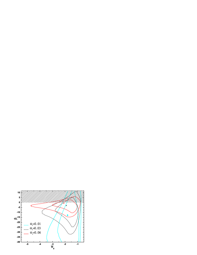
Figure 2: 2$\sigma$ SNIa limits on the coupled neutrino-DE model with neutrino mass evolving as $M_{\nu}=M_{\nu 0}(1+\beta u)$, where $u$ stands for $\ln a$. The dots inside show the best fit values. The cyan(light dashed), black(solid) and red(dark dashed) contours stand for $\Omega_{\nu}=0.01,0.03$ and 0.06 respectively. The hatched area denotes where the neutrino mass might be negative on large redshifts and physically forbidden. In the fittings we’ve applied the uniform prior $0.2<\Omega_{m}<0.4$.

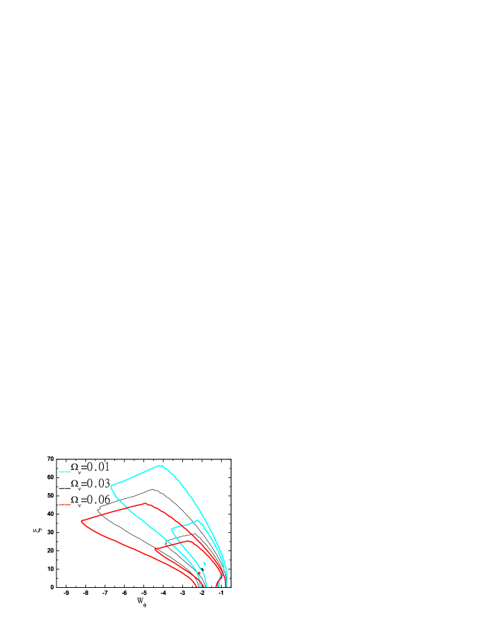
Figure 3: 2$\sigma$ SNIa limits on the coupled neutrino-DE model with neutrino energy density evolving as $\rho_{\nu}=\frac{\Omega_{\nu 0}}{\Omega_{\phi 0}}\rho_{\phi}a^{-\xi}$, where the subscript ’0’ stands for today’s value. The dots inside show the best fit values. The cyan(light dashed), black(solid) and red(dark dashed) contours stand for $\Omega_{\nu}=0.01,0.03$ and 0.06 respectively. In the fittings we’ve applied the uniform prior $0.2<\Omega_{m}<0.4$.

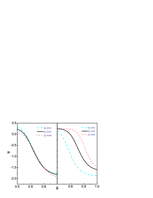
Figure 4: Effective EOS for the coupled neutrino-DE system for the best-fit values of the two models shown in Fig.2 and Fig.3. The cyan(dashed), black(solid) and red(dotted) lines stand for $\Omega_{\nu}=0.01,0.03$ and 0.06 respectively. The left panel stands for the model with $M_{\nu}=M_{\nu 0}(1+\beta u)$ and the right panel for $\rho_{\nu}=\frac{\Omega_{\nu 0}}{\Omega_{\phi 0}}\rho_{\phi}a^{-\xi}$.

With a uniform prior $0.2<\Omega_{m}<0.4$ in Fig. 2 we delineate 2$\sigma$ SNIa constraints on the parameter space $(\beta,w_{\phi})$ of our model, where the SNIa data are taken from the Riess Gold sample[1]. We can see that a non-vanishing $\beta$ is preferred and the data mildly favor the model where the neutrinos interact with the phantom-like scalar. The parameter space gets better constrained with the increase of $\Omega_{\nu}$. Normally we expect that the constraints of the parameter $\beta$ should be $\mid\beta\mid<1$ for the consideration of the small $\ln a$ expansion, but the current SNIa constraint is very weak which lead to the $\ln a$ expansion of $M_{\nu}$ in Eq. (22) loses its significance in some sense as a large $|\beta|$ is not ruled out and even somewhat favored. Moreover, the linear parametrization itself is not well defined for a large but positive $\beta$, because the neutrino becomes massless and even be with a negative mass on large redshifts. In our Fig.2 the hatched denotes where $\beta>0$. We should point out that in our numerical calculations we used no approximations and just set Eq. (22) as a parametrization.

Given the limitation mentioned above and the conventions in the literature for the parametrization of the EOS of dark energy one may consider different types of parametrization of the neutrino mass. For an example we consider here another type of parametrization which was firstly invoked for the study of dark energy coupled with dark matter in solving the coincidence problem[33]

$$\frac{\rho_{\phi}}{\rho_{\nu}}=Aa^{\xi},$$ (27)

where $A$ and $\xi$ are constant. $A$ is determined by $A=\frac{\Omega_{\phi_{0}}}{\Omega_{\nu_{0}}}$, and the variation of the neutrino mass is $d\ln M_{\nu}/d\ln a=-\frac{\Omega_{\phi_{0}}(\xi+3w_{\phi})}{\Omega_{\phi_{0}}+\Omega_{\nu_{0}}a^{-\xi}}$. Correspondingly we now get

$$E(a)=(1-\Omega_{m_{0}})a^{-3}(\frac{\Omega_{\nu_{0}}+\Omega_{\phi_{0}}a^{\xi}}{\Omega_{\nu_{0}}+\Omega_{\phi_{0}}})^{-\frac{3w_{\phi}}{\xi}}+\Omega_{m_{0}}a^{-3}.$$ (28)

There would be interactions between neutrinos and the scalar dark energy when $\xi\neq-3w_{\phi}$. $\xi=3,w_{\phi}=-1$ stands for the conventional non-interacting $\Lambda$CDM cosmology and $\xi=0$ for the ”tracking” neutrino which would behave the same as dark energy. As shown in Ref.[22] it is not applicable that neutrino and DE can enter the tracking regime as early as today, since neutrino takes up a very small density fraction and dark energy only comes to dominate the universe very recently. Hence we will restrict our attentions on the parameter space where $\xi>0$.

In Fig.3 we delineate the 2$\sigma$ SNIa constraints on the parameter space of $(\xi,w_{\phi})$. The cyan(light dashed), black(solid) and red(dark dashed) contours stand for $\Omega_{\nu}=0.01,0.03$ and 0.06 respectively. We can see that current SNIa constraints are very weak and the data favor mildly the model where neutrinos interact with the phantom-like scalar. It is noteworthy that here the best fitting values show $\xi+3w_{\phi}>0$, which corresponds to an increase of neutrino mass with the redshift, and the behavior is similar to our first example. We find for the two parametrizations when the prior of $\Omega_{m}$ is relaxed the parameter space would be constrained less stringently, but a phantom-like DE coupling with neutrinos is still mildly favored.

More recently the authors of Ref.[30] made the distance measurements to 71 high redshift type Ia supernovae discovered during the first year of the 5-year Supernova Legacy Survey (SNLS). SNLS will hopefully discover around 700 type Ia supernovas, which is an intriguing ongoing project. When performing the current SNLS constraints on the neutrino-DE coupling, we found that the current SNLS data have not yet been as precise as the Riess Gold sample[1] and the conclusion above has not changed.

As shown by Eq.$(\ref{whole w})$, for SNIa data only the preference for a Quintom-like behavior of dark energy (where the equation of state gets across -1) is fully degenerate with the preference of a coupling between neutrinos and phantom-like dark energy($w_{\phi}<-1$). In fact the fittings in Section II can also be rephrased as current SNIa constraints on the linearly parametrized EOS of single component of dark energy, as shown in Ref.[5]. To give a more intuitive example we delineate in Fig.4 the effective EOS of the full coupled system given by the best fit values of Fig.2 and Fig.3. The cyan(light dashed), black(solid) and red(dark dashed) lines stand for $\Omega_{\nu}=0.01,0.03$ and 0.06 respectively. The left panel stands for the model with $M_{\nu}=M_{\nu 0}(1+\beta u)$ and the right panel for $\rho_{\nu}=\frac{\Omega_{\nu 0}}{\Omega_{\phi 0}}\rho_{\phi}a^{-\xi}$. We can see they all show a Quintom-like behavior. Actually from Eqs.(26) and (28) we can easily work out the analytic forms of the effective EOS:

$$w = -1-\frac{1}{3D}\{\Omega_{\nu_{0}}a^{-3}(-3+\beta-3\beta\ln a)$$ (29)

$$+ \Omega_{\phi_{0}}[-3(B+1)(1+w_{\phi})a^{-3(1+w_{\phi})}$$

$$+ 3Ba^{-3}]\},$$

where

$$D=\Omega_{\nu_{0}}a^{-3}(1+\beta\ln a)+\Omega_{\phi_{0}}X(a),$$ (30)

and

$$B=\frac{\beta\Omega_{\nu_{0}}}{3w_{\phi}\Omega_{\phi_{0}}}$$ (31)

for the coupling form of Eq.(27) and

$$w=w_{\phi}\frac{\Omega_{\phi_{0}}a^{\xi}}{\Omega_{\nu_{0}}+\Omega_{\phi_{0}}a^{\xi}},$$ (32)

for the form of Eq.(28), which could easily get across the cosmological constant boundary for the given best fit values shown in Fig.2 and Fig.3.

The projected satellite SNAP (Supernova / Acceleration Probe) would be a space based telescope with a one square degree field of view with 1 billion pixels. It aims to increase the discovery rate for SNIa to about 2,000 per year[34]. In the following we will use the simulated three-year SNAP data to investigate to what an extent future SNAP would be able to detect or rule out the currently mildly favored couplings between dark energy and neutrino. In addition we assume a gaussian prior $\sigma_{m}=0.01$, it is close to future Planck constraints.

The underlying fiducial model used here is the uncoupled $\Lambda$CDM model with $w_{\phi}=-1,\Omega_{\phi}=0.7$ and $h=0.7$. It corresponds to $\beta=0$ in the coupling form of Eq.(22) and $\xi=3$ in the form of Eq.(27). The simulated SNIa data distribution for each year is taken from Refs. [35, 36]. As we consider 3-year data, the number for each bin will be improved by around $3$ times. As for the error, we follow the ref. [35] which takes the magnitude dispersion $0.15$ and the systematic error $\sigma_{sys}(z)=0.02*z/1.7$, and the whole error for each data is

$$\sigma_{mag}(z_{i})=\sqrt{\sigma_{sys}^{2}(z_{i})+\frac{0.15^{2}}{n_{i}}},$$ (33)

where $n_{i}$ is the number of supernova in the i’th redshift bin.

In Figure 5 we show the 3-year SNAP constraints on the coupled neutrino-DE model given by Eq.(22). The red(light dashed), blue(dark dashed) and green(solid) 2$\sigma$ contours stand for $\Omega_{\nu}=0.01,0.03$ and 0.06 respectively. We find the coupling parameter of $\beta$ is restricted to be of order unity and the parametrization of $\ln a$ has made its sense when the neutrino density fraction can be order of $0.01$.

Correspondingly in Figure 6 we delineate the 3-year SNAP constraints on the coupled neutrino-DE model given by Eq.(28). The red(dashed), blue(dash dotted) and green(solid) 2$\sigma$ contours stand for $\Omega_{\nu}=0.01,0.03$ and 0.06 respectively. The behavior of this parametrization is not symmetric around the fiducial $\Lambda$CDM model, and the constraints on the parameters are similar to that of the linear parametrization. Thus the future projects like SNAP can improve the precision efficiently and is potentially able to detect the couplings between neutrino and dark energy.

Figure 5: Simulated 3-year SNAP constraints on the coupled neutrino-DE model with neutrino mass evolving as $M_{\nu}(u)=M_{\nu}(0)(1+\beta u)$, where $u$ stands for $\ln a$. The red(dashed), blue(dash dotted) and green(solid) 2$\sigma$ contours stand for $\Omega_{\nu}=0.01,0.03$ and 0.06 respectively. The hatched area denotes where the neutrino mass might be negative on large redshifts and physically forbidden. The underlying fiducial model has been chosen as the uncoupled $\Lambda$CDM model with $c=0,w_{\phi}=-1,\Omega_{\phi}=0.7$ and $h=0.7$. We take a gaussian prior $\sigma_{m}=0.01$.

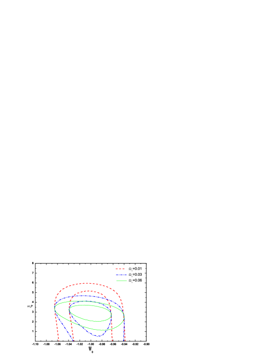
Figure 6: Simulated 3-year SNAP constraints on the coupled neutrino-DE model with neutrino energy density evolving as $\rho_{\nu}=\frac{\Omega_{\nu 0}}{\Omega_{\phi 0}}\rho_{\phi}a^{-\xi}$, where the subscript ’0’ stands for today’s value. The red(dashed), blue(dash dotted) and green(solid) 2$\sigma$ contours stand for $\Omega_{\nu}=0.1\%,0.01,0.03$ and 0.06 respectively. The underlying fiducial model has been chosen as the uncoupled $\Lambda$CDM model with $\xi=3,w_{\phi}=-1,\Omega_{\phi}=0.7$ and $h=0.7$. We take a gaussian prior $\sigma_{m}=0.01$.

IV Discussions and conclusion

In this paper we have made the first study on the constraints on the couplings between neutrinos and the scalar field of dark energy from current and future observations of SNIa. We have shown that the coupled system of neutrino dark energy can resemble the behavior of Quintom and is fully degenerate with Quintom in light of the geometric observations of SNIa only. A system with the phantom-like dark energy coupled to massive neutrino is mildly favored by current SNIa data where the neutrino mass is increasing with the redshift. Such couplings are promising to be detected by future observations.

V acknowledgements

Our simulations are computed in the Shanghai Supercomputer Center (SSC). We thank Pei-Hong Gu for helpful discussions and Jean-Marc Virey and A. Tilquin for helpful comments. This work is supported in part by National Natural Science Foundation of China (grant Nos. 90303004, 19925523) and by Ministry of Science and Technology of China ( under Grant No. NKBRSF G19990754).

References

- [1] A. G. Riess et al., Astrophys. J. 607, 665 (2004).
- [2] D. N. Spergel et al., Astrophys. J. Suppl. 148, 175 (2003).
- [3] M. Tegmark et al., Phys. Rev. D69, 103501 (2004).
- [4] B. Ratra and P. J. E. Peebles, Phys. Rev. D37, 3406 (1988); C. Wetterich, Nucl. Phys. B302, 668 (1988); C. Wetterich, Astron. & Astrophys. 301, 321 (1995); J. A. Frieman, C. T. Hill, A. Stebbins, and I. Waga, Phys. Rev. Lett. 75, 2077 (1995); I. Zlatev, L. Wang, and P.J. Steinhardt, Phys. Rev. Lett. 82, 896 (1999); P. J. Steinhardt, L. Wang and I. Zlatev, Phys. Rev. D59, 123504 (1999).
- [5] B. Feng, X. Wang and X. Zhang, Phys. Lett. B607, 35 (2005).
- [6] B. Feng, M. Li, Y.-S. Piao and X. Zhang, astro-ph/0407432; Z.-K. Guo, Y.-S. Piao, X. Zhang and Y.-Z. Zhang, Phys. Lett. B608, 177 (2005).
- [7] e. g. U. Alam, V. Sahni, and A. A. Starobinsky, JCAP 0406, 008 (2004); D. Huterer and A. Cooray, Phys. Rev. D71, 023506 (2005); S. Nesseris and L. Perivolaropoulos, Phys. Rev. D 70, 043531 (2004); S. Hannestad and E. Mortsell, JCAP 0409, 001 (2004); P. S. Corasaniti, M. Kunz, D. Parkinson, E. J. Copeland and B. A. Bassett, Phys. Rev. D70, 083006 (2004); D. A. Dicus and W. W. Repko, Phys. Rev. D70, 083527 (2004); B. A. Bassett, P. S. Corasaniti, and M. Kunz, Astrophys. J. 617, L1 (2004); Y. G. Gong, Class. Quant. Grav. 22, 2121 (2005); M. Doran and J. Jaeckel, Phys. Rev. D 66, 043519 (2002).
- [8] P. Q. Hung, hep-ph/0010126. This paper considers the interaction between the Quintessence and the steril neutrinos.
- [9] M. Li, X. Wang, B. Feng, X. Zhang, Phys. Rev. D65, 103511 (2002).
- [10] M. Li, X. Zhang, Phys. Lett. B573, 20 (2003).
- [11] P. Gu, X. Wang and X. Zhang, Phys. Rev. D68, 087301(2003).
- [12] R. Fardon, Ann E. Nelson and N. Weiner, JCAP 0410, 005 (2004).
- [13] P. Gu and X.-J. Bi, Phys. Rev. D70, 063511 (2004); X. Bi, P. Gu, X. Wang and X. Zhang, Phys. Rev. D69, 113007 (2004).
- [14] P. Q. Hung and H. Pas, Mod. Phys. Lett. A20, 1209 (2005).
- [15] D. B. Kaplan, A.E. Nelson, and N. Weiner, Phys. Rev. Lett. 93, 091801 (2004).
- [16] R. D. Peccei, Phys. Rev. D71, 023527 (2005).
- [17] V. Barger, P. Huber and D. Marfatia, hep-ph/0502196; M. Cirelli, M. C. Gonzalez-Garcia and C. Pena-Garay, Nucl. Phys. B 719, 219 (2005).
- [18] R. Horvat, astro-ph/0505507.
- [19] N. Afshordi, M. Zaldarriaga and K. Kohri, astro-ph/0506663.
- [20] R. Takahashi and M. Tanimoto, hep-ph/0507142.
- [21] H. Li, Z. Dai and X. Zhang, Phys. Rev. D71, 113003 (2005).
- [22] X. J. Bi, B. Feng, H. Li and X. m. Zhang, Phys. Rev. D 72, 123523 (2005).
- [23] X. Zhang, H. Li, Y. Piao and X. Zhang, astro-ph/0501652.
- [24] R. R. Caldwell, Phys. Lett. B545, 23 (2002).
- [25] For a relevant study see U. Franca and R. Rosenfeld, Phys. Rev. D69, 063517 (2004).
- [26] L. Conversi, A. Melchiorri, L. Mersini and J. Silk, Astropart. Phys. 21, 443, (2004).
- [27] S. Hannestad and L. Mersini-Houghton, Phys. Rev. D71, 123504 (2005).
- [28] J.-M. Virey et al., Phys. Rev. D70, 121301 (2004).
- [29] A. W. Brookfield, C. van de Bruck, D. F. Mota and D. Tocchini-Valentini, astro-ph/0503349.
- [30] P. Astier et al., astro-ph/0510447.
- [31] Y. Fukuda et al., Phys. Rev. Lett. 81, 1158 (1998); Y. Ashi et al., Phys. Rev. Lett. 93, 101801 (2004); E. Aliu et al., Phys. Rev. Lett. 94, 081802 (2005).
- [32] S. Hannestad, Phys. Rev. Lett. 95, 221301 (2005).
- [33] N. Dalal et al., Phys. Rev. Lett. 87, 141302 (2001); E. Majerotto, D. Sapone and L. Amendola, astro-ph/0410543.
- [34] http://snap.lbl.gov.
- [35] A. G. Kim et al., Mon. Not. R. Astron Soc. 347, 909 (2004).
- [36] Ch. Yeche et al., astro-ph/0507170.