A Comparison of the Chemical Evolutionary Histories of the Galactic Thin Disk and Thick Disk Stellar Populations

Abstract

We have studied 23 long-lived G dwarfs that belong to the thin disk and thick disk stellar populations. The stellar data and analyses are identical, reducing the chances for systematic errors in the comparisons of the chemical abundance patterns in the two populations. Abundances have been derived for 24 elements: O, Na, Mg, Al, Si, Ca, Ti, Sc, V, Cr, Mn, Fe, Co, Ni, Cu, Zn, Sr, Y, Zr, Ba, La, Ce, Nd, and Eu. We find that the behavior of [$\alpha$/Fe] and [Eu/Fe] vs. [Fe/H] are quite different for the two populations. As has long been known, the thin disk O, Mg, Si, Ca, and Ti ratios are enhanced relative to iron at the lowest metallicities, and decline toward solar values as [Fe/H] rises above $-1.0$. For the thick disk, the decline in [$\alpha$/Fe] and [Eu/Fe] does not begin at [Fe/H] = $-1.0$, but at $-0.4$. Other elements share this same behavior, including Sc, Co, and Zn, suggesting that at least in the chemical enrichment history of the thick disk, these elements were manufactured in similar-mass stars. The heavy $s$-process elements Ba, La, Ce, and Nd are over-abundant in the thin disk stars relative to the thick disk stars. On the other hand, the constancy of the [Ba/Y] ratio suggests that only one $s$-process site was manufacturing these elements, or, possibly, that the $r$-process was responsible for the bulk of the nucleosynthesis of these elements. We combine our results with other studies (Edvardsson et al., Prochaska et al., Bensby et al., and Reddy et al.), who had already found very similar trends, in order to further explore the origin of the thick disk. The signs for an independent (parent galaxy) evolution of the thick disk are clear, in terms of the different metallicities at which the [$\alpha$/Fe] ratios begin to decline, as well as “step function” behavior of some elements, including [Eu/Y], [Ba/Fe], and, possibly, [Cu/Fe], at [Fe/H] $\approx-0.2$.

1 INTRODUCTION

On the basis of star counts, Gilmore & Reid (1983) argued that the Galaxy contains a second disk population, with a larger vertical scale distribution and hotter kinematics than the “classical old disk”. This “thick disk”, as it is now commonly called, is of considerable relevance to the understanding of the evolution of our Galaxy and, by extension, other disk galaxies. Does the development of all disk galaxies involve such a thick disk and, if so, why? If the thick disk is such a “pre-destined” evolutionary stage, can we determine its relationship with the other Galactic stellar populations, including the halo, the thin disk, and the bulge?

Or does the thick disk of the Milky Way represent an entanglement or a merger with another, presumably much smaller, galaxy? If so, are such encounters stochastic and infrequent among disk galaxies or are such encounters expected as part of some sort of hierarchical assembly of large galaxies out of cannibalization of smaller ones?

The salient properties of the thick disk, and clues to answering these questions, include the relative masses of the thick and thin disks, the vertical scale height, the mean metallicity, the metallicity gradient, the kinematics, the age (and age spread, if one is detectable), and the chemical evolution. The last property is the subject of this paper, but, as we discuss, it is not independent of the others.

The mid-plane density normalization of the thick disk relative to the thin disk has been the subject of serious study since the thick disk’s discovery, and the subject is well reviewed by Chen et al. (2001). They employed the Sloan Digital Sky Survey to provide a comprehensive new attack on the problem, finding preferred vertical scale heights of between 580 and 750 pc for the thick disk, compared to 330 pc for the thin disk. Since density normalization is directly related to scale heights, this range in values implies mid-plane density normalizations of 13% down to 6.5%. It is worth recalling that heating over a long period of time of Galactic thin disk stars by spiral arms or a central bar, giant molecular clouds, or accretion and enlargement of the Galactic disk are unable to explain such a difference in the scale heights (Jenkins 1992; Asiain, Figueras, & Torra 1999; Fuchs et al. 2001).

The local mean metallicity, $<$[Fe/H]$>$, of the thick disk is between $-$0.5 and $-$0.7 (Gilmore & Wise 1985, Carney et al. 1989, Gilmore et al. 1995; Chiba & Beers 2000). The mean metallicity and spread are very similar to what is seen among the disk globular clusters identified by Zinn (1985; see also Armandroff 1989), and there is some evidence of a metal-weak tail extending down to [Fe/H]=$-$1.6 (Norris et al. 1985, Martin & Morrison 1998). Though the average metallicity of the thick disk is only one third that of the thin disk, and much higher than that of the halo, the metallicity ranges certainly overlap, making it difficult to separate the two components based solely on metallicity.

The thick disk may be most readily distinguished from the thin disk in kinematics. The asymmetric drift of the thick disk has been measured between 20 km s^-1 (Chiba & Beers 2000) and 50 km s^-1 (Carney et al. 1989). Soubiran et al. (2003) and Bensby et al. (2003) agreed well of the values for the asymmetric drift, $<$V$>$, and the velocity ellipsoid [$\sigma$(U):$\sigma$(V):$\sigma$(W)] of the Galactic thin disk, thick disk, and halo stellar populations, with $<$V$>$ $\approx$ $-15$, $-50$, and $-220$ km s^-1, and velocity ellipsoids of, approximately, (35:20:16), (67:38:35), and (160:90:90) km s^-1, respectively. These differences may be exploited to assign probabilities of membership in the thin disk, thick disk, and halo populations, and throughout this paper we follow the formulations employed by Venn et al. (2004).

A key property, and one overlooked occasionally, is that the thick disk appears to be about as old as the Galactic halo. Bensby et al. (2004b) have attacked the question of the relative ages of the thin disk and thick disk field stars, using field stars whose ages may be estimated individually, and whose population membership may be assigned probabilistically on the basis of kinematics. They find no evidence for age differences for thick disk stars with [Fe/H] $\leq-0.4$, but for the minority of stars more metal-rich than this limit, an age spread of several Gyrs may exist. As they noted, this is also consistent with the appearance of contributions by Type Ia supernovae at that metallicity level, and which we address also in this paper.

The Milky Way is not the only galaxy which possesses a thick disk population. Indeed, Dalcanton & Bernstein (2002) have found them in all of the 47 disk systems they surveyed. However, it is not clear if the envelopes they detected are thick disks or a galactic halo, because the limiting surface brightnesses they reached are comparable to where Zibetti, White, & Brinkmann (2004) have detected the appearance of faint spheroidal components. Nonetheless, the work of Dalcanton & Bernstein (2002) breaks new ground since earlier work did not reveal thick disks in all edge-on disk galaxies (Morrison, Harding, & Boroson 1994; Fry et al. 1999). The absence of thick disks in other galaxies would support the idea that thick disks arise from “accidents”, probably encounters with other galaxies, rather than being a natural part of the formation of a thin disk. However, as Dalcanton & Bernstein (2002) argued, the near-universality of thick disks does not necessarily mean that they arise independently of encounters. While it is true that the red colors of extra-galactic thick disks indicate great ages, consistent with the “monolithic” formation idea, the thick disks do not appear to show any correlations with the sizes of the thin disks, nor with the presence or absence of galactic bulges. Dalcanton & Bernstein (2002) suggested, instead, that thick disks could be expected from the hierarchical assembly of galaxies, in which case no such correlations would be expected. A particularly nice piece of work showing the dissimilarity between some thin and thick disk populations is that of Yoachim & Dalcanton (2005). We note that Dalcanton & Bernstein (2002) commented on the apparent similarity of the Galactic thick disk and thin disk stellar populations’ chemical abundance patterns rules out independent origins, a conclusion that now appears to have been premature, and which is the subject of our study.

2 THE ORIGIN OF THE THICK DISK

Several groups (Gilmore 1984; Wyse & Gilmore 1988; Sandage 1990; Burkert, Truran, & Hensler 1992; Pardi, Ferrini, & Matteucci 1995) have advocated that the thick disk was a precursor to the “old thin disk”, and thus a thick disk is a natural early step in the chemodynamical evolution of galactic disks. Burkert et al. (1992) argued for a rapid (300-400 Myr) thick disk formation phase. Such a rapid process would result in a thick disk with a very small age range and little or no metallicity gradient, as has been observed. However, such models predict a smooth transition to the thin disk predicting continuous age, [Fe/H], [X/Fe], and kinematic relationships.

Rather than a “pre-ordained” evolutionary scenario, the thick disk may have resulted from an encounter with a small galaxy, with a mass roughly like that of the Magellanic Clouds. Simulations by Quinn et al. (1993) and Sellwood, Nelson, & Tremaine (1998) have shown that a thick disk can form during a merger event by the heating of a pre-existing cold, thin disk. Because the old disks are wrecked in the merging process, any thin disk we see today would have re-formed after the merger event, and the thick disk would be older than the bulk of the oldest stars in the reincarnated thin disk.

A thick disk may also form by the direct accretion of stars from the merging galaxy. Such a view was offered by Statler (1988), whose model involved the accretion of a “mature”, mostly stellar, galaxy. Statler showed that accretion can give rise to a boxy distribution similar to a thick disk, though this requires special initial conditions for the cannibalized galaxy’s orbit. In merger models there need not be continuity between the kinematics or chemical abundances of the thick and thin disks.

Distinguishing between evolutionary models and merger models requires age, kinematic, and abundance data for the halo, thick disk, and thin disk, especially at the transitions between the populations. Carney, Latham, & Laird (1989) argued that the thick disk is too distinct in its chemodynamical behavior, manifested, for example, by [Fe/H] vs. $|$W$|$ velocity, to share a common origin with the thin disk. Instead, they argued that the thick disk is likely to have arisen from a merger event, but a major one that involved already-assembled galaxies. The star formation in the victim may have been largely completed long before the actual merger.

3 TESTS OF THE MODELS

Mixing of stars from an accreted galaxy into the Milky Way, and scattering of stellar orbits via encounters with spiral arms, the central bar, or giant molecular clouds, will blur the kinematic signatures of a merger event. The orbital angular momentum, represented in the solar neighborhood by the Galactic V velocity, may be the best conserved kinematic property. In addition, stars retain the history of star formation in their abundance patterns, what Freeman & Bland-Hawthorn (2002) have called “chemical tagging”.

An ensemble of gas and stars should initially yield stars whose abundance patterns reflect only the ejecta from SNe II, which is thought to be the main production site of the $\alpha$-elements (O, Mg, Si, Ca, Ti) and $r$-process elements. SNe II arise from relatively massive stars, and hence the timescale for the appearance of their ejecta should be $\approx\ 10^{7}$ years. Low-mass (M $<$ 4 M_⊙) AGB stars are thought to be a major production site for $s$-process elements (Busso et al. 1999), and such stars begin releasing these elements into the ISM in about $10^{8}$ yrs, significantly later than $r$-process elements from SNe II. The $r$- to $s$-process ratio should therefore be higher at the earliest epochs in a population’s history and the metallicity where this ratio begins to decrease can give a star formation rate time-scale. SNe Ia begin to appear even later, perhaps within about $10^{9}$ years (see Matteuchi & Recchi 2001), and if star formation is slow enough for their ejecta to be incorporated into gas still undergoing star formation, the signature should appear at the mean metallicity the interstellar medium and newly-forming stars had reached. This is the basic explanation for the enhanced abundances of $\alpha$- elements seen in stars in the solar neighborhood at the lowest metallicities, and the steady decline in [$\alpha$/Fe] abundances from [Fe/H] $\approx$ $-1.0$ and higher. In other words, the solar neighborhood interstellar medium had reached a mean metallicity of [Fe/H] $\approx$ $-1$ before the SNe Ia began to significantly enrich the interstellar medium. Had star formation been more rapid, the metallicity would be higher before the SNe Ia contribution begin to appear. Thus one possible test of the inter-relationship between thin disk and thick disk populations is whether they share a common [$\alpha$/Fe] vs. [Fe/H] relation. If they do, the common history model is strengthened. If they do not, then one must either conclude that the thick disk evolved independently of the thin disk, or that the chemical enrichment models of the joint thick disk-thin disk evolution are much more complicated.

4 PRIOR WORK

One of the pioneering papers in this field is that by Edvardsson et al. (1993), who studied the abundances of 13 elements in 189 relatively bright, nearby dwarf stars. The stars were selected so that the sample covered a wide range in [Fe/H], and with an admixture of some halo population stars, judged by both metallicity and kinematics. The stars were also selected so that ages could be estimated for individual stars, and that those ages covered a very wide range, from less than 1 Gyr to roughly the age of the halo. Photometric metallicities enabled them to select stars on the basis of a range of ages. The kinematical data (proper motions and radial velocities) led to the caculation of space velocities and Galactic orbits, a truly comprehensive approach to the problem of the Galaxy’s chemodynamical evolution. At the risk of doing injustice to such a major piece of work, we summarize their three primary results briefly as the following. 1. As had been described earlier (see Wheeler, Sneden, & Truran 1989), [$\alpha$/Fe] is elevated by about 0.3 dex with respect to the Sun for stars with [Fe/H] $\leq\ -1.0$, but that it declines as a function of [Fe/H] for higher metallicities, reaching a solar value at [Fe/H] = 0.0. 2. This trend appears to depend on the mean Galactocentric distance of the stars involved. The trend is different for stars with smaller mean Galactcocentric distances, which could be explained by a higher star formation rate in the denser inner regions of the Galactic disk. We point out that thick disk stars in the solar neighborhood, with larger values of the asymmetric drift, may also have smaller mean Galactocentric distances, and hence the interpretation of these results could also be explained by a separate chemical evolutionary history for the thick disk rather than provide insight into the chemical evolution of the Galactic disk itself. 3. The Galactic disk does not appear to reveal an age-metallicity relation, as simple models of chemical evolution predict. The explanation offered most readily is that this might be explained by a combination of vigorous mixing of supernovae ejecta within the disk and infall of metal-deficient gas into the solar neighborhood. An alternative not considered by Edvardsson et al. (1993), but recently raised by Bensby, Feltzing, & Lundström (2004b), is that the lack of a correlation between age and metallicity could have resulted from a sample that inter-mixed two populations with differing mean metallicities and differing age-metallicity relations.

One good example of the challenges of target selection is the work of Chen et al. (2000). They studied 90 disk dwarfs with accurate parallaxes and kinematical data, and for which they could estimate ages for individual stars. They found that stars that kinematically resemble the thick disk follow a very similar trend in [$\alpha$/Fe] vs. [Fe/H] as do the stars of the thin disk. This supports the evolutionary model. However, the temperature regime for their target stars essentially rules out any long-lived stars in their sample, and if age is indeed a defining characteristic of the thick disk, then their adopted sample of thick disk stars may have simply included stars from the higher velocity tails of the thin disk velocity distributions. Thus the apparent agreement between the chemical evolution of the thin disk and thick disk may be spurious.

Gratton et al. (2003) added kinematics to the chemical abundance analyses of about 200 stars from Carretta, Gratton, and Sneden (2000). Their careful analyses, especially in the difficult matter of oxygen abundances, confirmed the onset of the decline in [O/Fe] at [Fe/H] $\approx\ -1.0$ for halo stars. However, their program stars were drawn from a wide variety of sources, so selection effects are hard to disentangle, and the ages of individual stars were not considered.

Fuhrmann (1998) initiated a large program of chemical abundances analyses of nearby F and G stars, mostly dwarfs but extending to subgiants near the main sequence turn-off. He employed kinematics (in a manner not well described) to distinguish between thin disk, thick disk, and halo stars, and was among the first to notice that the thick disk stars do not appear to follow the same [Mg/Fe] vs. [Fe/H] trend as do thin disk stars. His work has been continued by Mashonkina & Gehren (2000, 2001, 2003) in studies of [Ba/Fe] and [Eu/Fe] in the first two studies, and of more metal-poor stars in the last study. They confirmed differences in the [X/Fe] vs. [Fe/H] trends of thick disk vs. thin disk stars. Fuhrmann (2004) also undertook a comprehensive re-evaluation of the relative ages of the thin and thick disks based on a sample of roughly 150 field stars, concluding that the thick disk represents the first stage of the formation of the Galactic disk, and that a hiatus of perhaps 3 Gyrs ensued prior to the chemical evolution of the thin disk. A recent comprehensive literature study by Soubiran & Girard (2005) suggests a similar age difference, and confirms again the separate chemical enrichment histories of the two populations.

A much smaller sample, only ten stars, was studied by Prochaska et al. (2000). However, these stars were selected on the basis of both kinematics and “ages”, in the form of life expectancies that equal or exceed the age of the Galaxy, thereby minimizing the dilution of the sample by younger, hence thin disk, stars, which we have noted afflicted the study by Chen et al. (2000). Venn et al. (2004) confirmed the high probability of thick disk membership for all ten stars. A potential systematic effect may exist, however, since Prochaska et al. (2000) did not analyze a similar sample of thin disk stars. Possible differences in adopted $gf$ values or other analytical techniques raise the possibility of systematic effects creating differences where none exist or, alternatively, blurring or even erasing them when they do exist. Prochaska found that the thick disk behaves differently than the thin disk, supporting the accretion model, especially in the abundances of the $\alpha$ elements and the $r$-process element europium, a result obtained as well by Mashonkina et al. (2003).

Reddy et al. (2003) analyzed a much larger sample, 181 F and G dwarfs, studying abundances of 27 elements that span the critical classes of nucleosynthesis: CNO, $\alpha$, iron-peak, $s$-process, and $r$-process. The stars were selected employing kinematics and ages as the primary criteria, and the large majority of their stars belong to the thin disk. While they also noted different chemical evolutionary behaviors between the thin disk and the thick disk, perhaps their most important result was clear evidence for the expected thin disk age-metallicity relation with the remarkably small scatter in the relation. This suggests that the study of Edvardsson et al. (1993) may indeed have been compromised by mixing of the thin disk and thick disk in uncertain proportions.

In our opinion, the most important ensemble of studies regarding the chemical evolution of the thin disk and thick disk populations are those of Feltzing, Bensby, & Lundström (2003), Bensby, Feltzing, & Lundström (2003, 2004a, 2004b), and Bensby et al. (2005). These authors studied a sample comparable in size to those of Edvarsson et al. (1993), but were careful to distinguish thin disk and thick disk stars on the basis of their kinematics, using adopted mid-plane density ratios, asymmetric drifts, and velocity ellipsoids. Further, their sample covered a critical range of metallicities, including thick disk stars at the higher metallicities than have been traditionally, but probably incorrectly, assumed to be “reserved” to the thin disk, [Fe/H] $>$ $-0.5$. Bensby et al. (2003, 2004a, 2005), found, as had others, that the thick disk and thin disk populations begin to diverge in [$\alpha$/Fe] vs. [Fe/H] for key elements at [Fe/H] $\approx\ -1.0$, with the thin disk [$\alpha$/Fe] declining while the thick disk [$\alpha$/Fe] values remain constant. Further, they also found that the thick disk population also begins to show a decline in [$\alpha$/Fe] toward solar values beginning at [Fe/H] $\approx\ -0.4$. Thus the metal-rich tail of the thick disk appears to have formed long enough after the onset of star formation for SNe Ia to contribute their ejecta to the remaining gas, or, perhaps, that the remaining gas was mixed into a larger reservoir in which the [$\alpha$/Fe] ratio was already reduced. We have noted above that Bensby et al. (2004b) found that even among the stars in their sample most likely to belong to the thick disk (their TD/D $>$ 10 sample), the most metal-rich stars appear to be several Gyrs younger than the more metal-poor stars.

Finally, Mishenina et al. (2004) obtained abundances for magnesium and silicon ($\alpha$ elements), as well as iron and nickel, in 174 F, G, and K dwarfs, and confirmed the break in the [$\alpha$/Fe] vs. [Fe/H] of the thick disk at [Fe/H] $\approx\ -0.5$, and that the thin disk and thick disk are chemically distinct. Unfortunately, none of their program stars had estimated ages, and some of the stars appear to have relatively short life expectancies.

5 OBSERVATIONS

5.1 Target Selection

We have selected our targets for abundance determinations following an unpublished study by Nauomov (1999) of the Galaxy’s thin disk and thick disk stellar populations. His work comprised two parts. In the first, he undertook an exhaustive review of all available uvby photometry and parallax data and he selected dwarfs generally lying within 100 pc of the Sun. Temperatures were determined using the color-temperature calibrations of Alonso, Arribas, & Martinez-Roger (1996). Nauomov employed the Olsen (1993) catalogue in an unbiased manner, selecting all stars with with $b-y$ $\geq$ 0.4, corresponding to stars cooler than $\approx$5700 K, and having life expectancies on order of the thick disk’s age. This criterion was chosen based on the estimated turn-off temperature of 47 Tuc, and resulted in a sample of 269 stars.

In the second part, Nauomov obtained objective prism spectra near the Galactic mid-plane using narrow-band interference filters to enable classification of stars as faint as $V\approx 11$ mag. Spectral indices enabled him to distinguish dwarfs from giants, and to determine effective temperatures. Again, there were no selection effects that might bias the sample in favor of thin disk or thick disk stars on the bases of either kinematics or chemistry. Short-exposure direct imaging CCD observations taken with the same telescope produced $V$ magnitudes and $V-I_{C}$ color indices. Nauomov compared the temperature estimates from the reddening-independent line indices and the observed $V-I_{C}$ colors to estimate the reddening for each star. This second sample was likewise trimmed so that only long-lived stars remained.

The resultant sample, comprising roughly 1200 stars near the Sun or at least near the Galactic plane, was then studied using the Center for Astrophysics radial velocity speedometers. From these spectra, Nauomov was able to determine radial velocities with individual measurement precisions of better than 1 km s^-1. Further, with confidence that all the program stars are dwarfs, and with knowledge of the temperatures, Nauomov could determine mean metallicities following the procedures described by Carney et al. (1987, 1994) and Laird et al. (1988). Figure 2 shows the results for the stars selected from the Olsen (1993) catalog, as well as the stars selected from the objective prism observations with $\ell\approx 90$ and $b\approx 0$, so that the radial velocity is a direct measure of the V velocity. The Figure merits careful consideration. As expected, one sees the thin disk with $<$V$>$ $\approx$ 0 km s^-1, and dispersion of order 20 km s^-1. The thin disk range in [Fe/H] is approximately from $-1$ to slightly above solar. Note that there are very few stars in the Figure with V velocities as high as +50 km s^-1, but a considerable number with V $\approx-50$ km s^-1. That excess, we believe, represents the thick disk.

In Figure 3 we show the V velocity histogram for stars with $-1.0\leq$ [Fe/H $\leq\ -0.3$. The thick disk signature is distinct, with a peak, as expected, near $-50$ km s^-1, and it is clear that the thick disk is a minor component near mid-plane, consistent with the results of Chen et al. (2001).

From Figure 2 we note also that the thin disk and the thick disk stars do not appear to overlap in the V vs. [Fe/H] plane at any location. The thick disk stars appears to maintain a characteristic signature V velocity at all values of [Fe/H]. This supports an independent origin, presumably later involving accetion, for the origin of the thick disk, and that it is not an antecedent to the thin disk. For the purposes of this paper, Figure 2 also enables us to select our program stars. We chose to limit our subsequent studies of stars to those with $uvby$ photometry.

We re-calculated U, V, and W velocities for the 269 stars in Naumov’s (1999) sample based on parallaxes and proper motions from the Hipparcos Catalogue (Perryman et al. 1997) and his and new radial velocities from Latham et al. (2002 and private communication). Since the most distinctive kinematic signature of the thick disk is its asymmetric drift, we used V velocities as a primary selection criterion. We employed a “Toomre diagram” that plots the V velocity against the combined U and W velocities, as shown in Figure 4. The distance from the origin in such a diagram is a measure of a star’s energy of motion, itself also an approximately conserved quanitity. Stars were also chosen on the basis of scientific goals, in the sense that we wished to have comparable numbers of thin disk and thick disk stars, that they span similar ranges of metallicity, and that all stars have similar effective temperatures to minimize any potential systematic effects in our analyses.

We assigned nine of our program stars to the thin disk and fourteen stars to the thick disk. Open circles in Figure 4 depict stars we classifed as belonging to the thin disk, while filled circles represent the thick disk candidates. Subsequent to this, well after the observing and analyses had been completed, we attempted a more quantitative population membership assignment. We followed the prescriptions of Venn et al. (2004) to assign such membership probabilities, which are given in Table 3. All nine stars assigned by our selection criteria to the thin disk appear to be members, with probabilities exceeding 75% in all cases. For the thick disk assignments, membership assignments are less clear for several stars, including BD+65 3 (only 51%) and BD+13 1655 (only 57%). We retain these stars as thick disk candidates throughout this work, however.

We present the basic data for our program stars in Tables 1, 2, and 3. Table 1 summarizes the radial velocity data obtained using the CfA speedometers. The summary includes the number of observations, N, the span (in days), the mean radial velocity and its associated error of the mean, the “external” error, E, derived from the individual velocities, the “internal” error, I, estimated from the ratio of the height of the peak in the power spectrum to the mean noise level, and the ratio E/I. Values above 1.5 generally indicate velocity variability. A better indicator is $P$($\chi^{2}$), the probability that the resultant value of $\chi^{2}$ could have arisen from the internal errors. A sample of constant-velocity stars should show a uniform distribution of $P$($\chi^{2}$). As the Table reveals, five of our program stars have very small $P$($\chi^{2}$) values, and are single-lined spectroscopic binaries, a more-or-less typical fraction seen among field stars, independent of metallicity (see Latham et al. 2002). Table 2 summarizes the available photometry for our program stars, including $JHK$ photometry from the 2MASS survey. In Table 3 we summarize the metallicity and temperature estimates obtained from the photometry, and our calculated Galactic UVW velocities.

Because the stars in this study are more metal rich than 47 Tuc, we compared our stars’ temperatures and metallicities with the model isochrones of Kim et al. (2002) to ensure that these stars are unevolved and have life expectancies of at least 10 Gyr. Temperature estimates from both Strömgren photometry and $V-K$ colors using 2MASS data were employed to calculate the stellar effective temperatures, again relying on the color-temperature relations of Alonso et al. (1996).

5.2 Observing Runs & Data Reductions

We obtained high resolution echelle spectra for each star. The majority of the data were taken with the echelle spectrograph on the 4m Mayall telescope at Kitt Peak . To obtain the necessary large wavelength range, each star was observed with two different set-ups, one for the red end of the spectrum and one for the blue end. Both set-ups included the 31.6 grooves mm^-1 echelle grating, a 2048 x 2048 CCD chip with 24 $\mu$m pixels, and the T2KB long camera. The red set-up used the 226-1 cross disperser and the long red camera. The blue set-up used the 226-2 cross disperser in the second order, the long blue camera, and was binned by 2 in the spatial direction. The stellar spectra were taken with a 1″ slit and a 2.9″ decker, while the flats were taken with a 4″ decker. Both setups gave continuous coverage throughout the wavelength range with a resolving power of R = $\lambda/\Delta\lambda$ = 32,000.

Higher resolution (R = 60,000) spectra were also acquired by Inese Ivans using the 2.7m Harlan J. Smith telescope at McDonald Observatory using the “2d-coudé” echelle. The spectrograph was set in the cs23-e2 configuration and employed a Tektronix 2048 x 2048 chip with 24 $\mu$m pixels and a 1″ slit. The wavelength coverage is continuous at the blue end, with increasing inter-order gaps starting at $\approx$ 5700 Å. Table 4 gives the dates and wavelength coverage for each observing run. Table 5 gives the observing dates, total exposure time in minutes, and S/N per resolution element for each stellar spectrum. These are cited at 4130 Å and 6645 Å, which are near key lines of the $r$-process element europium. These are not at the centers of their orders’ blaze, and so are representative of a typical S/N level, and perhaps an underestimate in the blue region. Each spectrum has continuous wavelength coverage from 3900-7400 Å.

Standard echelle spectra reduction was undertaken using tools running inside the IRAF environment (Tody 1986). Bad pixels were interpolated over and the overscan region was trimmed. A set of projector flats was taken each night, averaged, and applied to the spectra. A fit to the overscan region was used for bias subtraction. Scattered light was removed by subtraction of a low-order surface fit to the inter-order light. The spectra were extracted, continuum flattened, and normalized. Thorium-argon lamp comparison spectra were used for wavelength calibration of the data. Each run also included spectra of hot, rapidly rotating stars to aid in the removal of telluric lines. Each such spectrum used in the analysis of any program star was taken at a comparable airmass, and always had S/N levels of over 500 per resolution element. We took care to measure equivalent widths before and after the division to be certain that this calibration step did not itself introduce errors into our results.

6 ANALYSES

6.1 Spectroscopic Atmospheric Parameters

The Fe I and Fe II lines were used to set the atmospheric parameters: effective temperate ($T_{\rm eff}$), surface gravity (log g), and microturbulent velocity ($\xi$). Our list of iron lines comes from Prochaska et al. (2000). In general, their spectra were of higher resolution than ours, and several of the lines they employed were blended in our spectra and had to be discarded. Lines were used only if they were measurable in at least two of our program stars. Equivalent widths for each line were measured in the SPLOT package of IRAF, using a Gaussian profile for weak lines ($\leq$ 40 mÅ) or a Voigt profile for stronger lines. Lines stronger than 150 mÅ were not employed in our analyses, since they generally form at such shallow depths that we have greater concerns about the validity of the LTE model atmosphere $T-\tau$ relations.

ATLAS9 (Kurucz 1993) was used to produce plane-parallel, atomic and molecular line-blanketed, flux-conserving stellar models. Local thermodynamic equilibrium (LTE) was assumed throughout the stellar atmosphere. WIDTH9 was used, along with the Kurucz model atmospheres, to derive an elemental abundance from each line. At the temperatures of our program stars, the equivalent widths of weak Fe I lines are relatively unaffected by changes in log g and $\xi$, so they were used to set $T_{\rm eff}$. Using only Fe I lines weaker than about 40 mÅ, the slope of the derived Fe I abundance versus excitation potential ($\chi$) was determined. If the slope deviated from zero by more than 50% of the uncertainty of the slope, a new model atmosphere was computed with a different temperature, and the process was repeated until the slope was, effectively, zero. The typical uncertainty in the slope for our stars translates to $\sigma$($T_{\rm eff}$) $\approx$ 60 K. With the temperature set, $\xi$ was found using all Fe I lines and repeating the analyses until the slope of abundance versus W_λ/$\lambda$ was zero to well within the uncertainty, with $\sigma$($\xi$) $\approx\ 0.1$ km s^-1.

The surface gravity was then found by requiring that the abundances from Fe I lines and Fe II lines agree. Again, if the results disagreed, a new model atmosphere was computed, and the iterations continued until the two species gave an iron abundance agreement within 0.01 dex. Based on the uncertainties in the Fe II abundances, we estimate the typical internal uncertainty in log g (excluding systematic effects such as the $gf$ values) to be 0.05 dex. A case has been made for systematic effects due to the failure of the LTE approximation (Thévenin & Idiart 1999), but the effects are likely to be very small for metal-rich dwarfs (Korn, Shi, & Gehren 2003). With these values of $T_{\rm eff}$, $\xi$, and log g, a final model atmosphere was produced with ATLAS9, and this model atmosphere for each star was then used in all subsequent abundance analyses. The final atmospheric parameters for each star are listed in the Table 6, which gives the $T_{\rm eff}$, metallicity, $\xi$, and log g of the model atmosphere and the derived Fe I and Fe II abundances, the number of absorption lines used for each, and the standard deviation of the abundances from individual absorption lines from the mean abundance.

Figures 5 and 6 compare the effective temperatures derived spectroscopically to those from the photometry. On average, the spectroscopic temperatures are 48 K higher ($\sigma$ = 47 K) than those from estimated using Strömgren photometry and 71 K ($\sigma$ = 57 K) higher than those obtained using $V-K$. We have used the relations derived by Schuster & Nissen (1989) to estimate [Fe/H] photometrically, and Figure 7 compares the the results with our spectroscopic values. Agreement is remarkably good, with no significant offset with and a remarkably small scatter of $\sigma$ = 0.11 dex.

6.2 Elemental Abundances

The abundances for 23 other elements were found using the adopted Kurucz model atmospheres and measured equivalent widths. As in the case of the iron lines, the equivalent widths were measured using SPLOT in IRAF employing a Gaussian or Voigt profile, depending on the strength of the line. Atomic parameters were taken primarily from the sources cited by Prochaska et al. (2000), with $gf$ values for several of the neutron-capture elements taken from Cowan et al. (2002). The wavelengths, excitation potentials, and $gf$ values of the lines are given in Table 7 along with the measured equivalent widths for each star. We adopted the photospheric solar abundances of Grevesse & Sauval (1998) with the exception of iron, for which the meteoritic value of log $\epsilon$ = 7.51 (Anders & Grevesse 1989) was chosen in order to match that adopted by Edvardsson et al. (1993). This value was also derived directly from our own photospheric abundance analysis of a solar spectrum using the same lines and $gf$ values employed for our program stars (see Section 6.3 and Table 9. It is only 0.01 dex larger than that obtained by Grevesse & Sauval (1998).

6.2.1 Hyperfine and Isotopic Splitting

Isotopes with an odd number of protons or neutrons exhibit hyperfine splitting of their spectral lines. Hyperfine interactions split the lines into multiple components with typical separations of a few mÅ. The splitting of the lines inhibits saturation of strong lines and must be taken into account to accurately derive the abundances from these lines, since, in general, abundances are overestimated if hyperfine splitting is ignored. Elements that have more than one stable isotope also exhibit isotopic splitting of their lines, and each isotope may have a slightly different set of hyperfine splitting. For our analyses, we adopted solar isotopic ratios from meteoritic values (Anders & Grevesse 1989). The wavelength of the hyperfine transitions and the relative $gf$ strengths were taken from Prochaska et al. (2000) for V, Co, Mn, Sc, and Cu, McWilliam (1998) for Ba, Kurucz (1995) for Eu, and Aoki et al. (2001) for La.

The software package MOOG (Sneden 1973) was used, in the synthesis mode $blends$, to derive abundances for these elements.

6.2.2 Synthetic Spectra

Three of the Eu lines and three of the La lines are in portions of the spectrum where line blending makes it impossible or at least unwise to measure simple equivalent widths. For these lines, abundances were found by comparison with synthetic spectra. MOOG was used to create a synthetic spectra of about 10 Å surrounding the line. The atomic and molecular line lists come from Kurucz (1995). Hyperfine and isotopic splitting were taken into account. The stellar spectrum was compared to the synthetic spectrum, and the abundance of the element was changed until the best fit was found. Figures 8 and 9 show examples of the synthetic spectra fit for one of our program stars using three different abundances. The (solid) middle line is the best fit to the stellar spectrum with the other lines representing changes of $\pm 0.1$ dex in the [La/H] and [Eu/H] abundances, based on $\chi^{2}$ goodness-of-fit measures supplied by MOOG.

6.2.3 Damping

Atomic line broadening by van der Waals damping was employed in our abundance analyses. A correction factor of 3 was multiplied to the Unsöld (1955) approximation for the damping constant for Ba as suggested by Holweger & Muller (1974) because the fit to the line with synthetic spectra is better than with the uncorrected damping factor. For all other elements the no multiplicative factor was included.

6.3 Error Analysis

There are several factors that affect the accuracy of our elemental abundances. Uncertainties in $gf$ values produce random errors in the results, but possible systematic effects as well. Laboratory values may have systematic effects that depend on the excitation potentials of the lower energy levels, for example. However, such should not alter the relative abundances of our own program stars, so the comparisons between our thin and thick disk program stars should be independent of these uncertainties. The uncertainties in the atmospheric parameters and the equivalent width measurements affect the internal uncertainty of our elemental abundances and are a measure of the ability to compare our thin and thick disk stars. [Fe/H] is most strongly affected while element-to-iron ratios are less sensitive, especially for elements whose ionization potentials are similar to that for iron (7.90 eV). We illustrate the effects of these uncertainties using BD+34 927, a star in the middle of the sample in both $T_{\rm eff}$ and metallicity. We calculated elemental abundances using eight different atmospheric models. The temperature was varied by $\pm$80 K, $\xi$ by $\pm$0.1 km s^-1, log g by $\pm$ 0.05, and [Fe/H] by $\pm 0.1$ dex. Table 8 summarizes the results.

Our abundance analyses, like essentially all of those discussed in Section 4, are relative to solar values, which, as noted above, were based on those derived from solar photospheric measures of Grevesse & Sauval (1998). In Table 9 we summarize the results we obtained using our adopted $gf$ values, and a solar model calculated using ATLAS9 with $T_{\rm eff}$ = 5770 K, log g = 4.44, and $\xi=1.15$ km s^-1. Columns 2 and 3 list the results from Grevesse & Sauval, in units of log $\epsilon_{\odot}$(X) = log $N_{\rm X}$ $-$ log $N_{\rm H}$ + 12.00, and our derived values of [X/H], relative to those values. Column 4 lists the individual scatter per line, and column 5 provides the number of lines employed. The solar spectrum was a lunar spectrum, obtained with the same instrumentation as used for our program stars, and reduced in an identical fashion. The agreement is excellent, except perhaps for vanadium and manganese. This result was expected since we have largely adopted $gf$ values from Prochaska et al. (2000), and they found similar underabundances for these elements. This suggests systematic errors may exist for our adopted $gf$ values for these elements, or the manner in which we have corrected for hyperfine splitting, or both. Fortunately, neither V nor Mn are critical for the comparisons of the thin disk and thick disk stellar populations.

The final elemental abundances for each star are listed in Tables 10 and 11. We include the standard error, per line, $\sigma$, and the number of lines used, $N$. For plotting purposes we rely on the mean error, defined as $\sigma/\sqrt{N}$. However, uncertainty propagates into the determination of $\sigma$ as well, especially when the number of lines employed is small, and for plotting purposes, we have resorted to an alternative method to estimate $\sigma$.

The random uncertainty in the abundance obtained using a single line may be estimated from from the uncertainty in the equivalent width measurement, following Cayrel (1989). The uncertainty in a measured equivalent width is estimated to be

$$\sigma(W_{\lambda})\approx\frac{\sqrt{FWHM\cdot\Delta x}}{S/N}$$ (1)

where $\Delta x$ is the dispersion in Å pixels^-1 and FWHM is the width of the spectral line in Å. For our spectra, $\Delta x\approx 0.05$ and FWHM ranges from 0.15 to 0.20 depending upon the strength of the line. Using S/N = 75 for the blue spectra and S/N = 150 for the red spectra, we find $\sigma(W_{\lambda})$ = 2 mÅ and 1 mÅ respectively. Most of our line measurements are from the red spectra, but $\sigma(W_{\lambda})$ does not take into account the difficulties in continuum placement, so we use an uncertainty in our equivalent width of 2 mÅ  which corresponds to an estimated abundance uncertainty of $\approx$ 0.05 dex.

In the Figures we have therefore employed the larger of 0.05/$\sqrt{N}$, following the discussion above, if N $<$ 5, or the error of the mean of the results from the individual lines if N $\geq$ 5. All elements whose abundances are based on a single line therefore have are therefore plotted with an error bar of 0.05 dex. This obviously neglects uncertainties in the $gf$ values themselves, which are hard to quantify.

7 RESULTS

The element-to-iron ratio of each element is plotted as a function of [Fe/H] in Figures 10 - 15, with thick disk stars identified by filled squares and thin disk stars by open squares. The error bars for each point are the internal uncertainties based on the scatter in the abundance values from the individual absorption lines. The abundance uncertainties due to uncertainties in atmospheric parameters are shown in the upper right corner of each figure.

7.1 Alpha-elements

Oxygen abundances for 13 stars were found from the 7774 Å triplet. The other 10 stars did not have spectral coverage in this region. Abundances from the 7774 Å triplet are very sensitive to effective temperature and non-LTE effects. (See Kiselman 1993 for a discussion of 1-d calculations and Kiselman & Nordlund 1995 and Asplund 2004 for calculations involving 3-d models.) Because our stars are fairly cool and cover a small range in atmospheric parameters, we assume that non-LTE effects would affect all of our program stars to comparable levels. Thus internal comparisons between the thin disk and thick disk stars in our sample should be robust, and any derived differences between the two populations should be real, even if the absolute oxygen abundances are less reliable. Figure 10 shows the [O/Fe] abundances for our stars and a clear difference in the thin and thick disk patterns. The thin disk oxygen abundances are on a plateau, [O/Fe] $\approx$ +0.2, or perhaps rising slowly with declining [Fe/H], for [Fe/H] $<-0.2$. At higher [Fe/H] values, the thin disk [O/Fe] descends to solar abundances. The thick disk abundances, on the other hand, are much higher, reaching [O/Fe] values of $\approx$ +0.6 for [Fe/H] $<-0.5$, and at higher [Fe/H], [O/Fe] declines toward solar values. At [Fe/H] =$-$0.4 there is about a 0.2 dex difference in the thick and thin disk abundances.

The abundances of Mg, Si, Ca, and Ti in Figure 10 all show the same pattern. For all the $\alpha$-elements, the thick disk stars with [Fe/H] $<-$0.4 show enhancements over the thin disk stars of the same metallicity. In the range $-$0.4 $<$ [Fe/H] $<-0.2$, the [$\alpha$/Fe] abundances in the thick disk stars decline steeply with increasing metallicity. While this decline is most apparent in the Mg and Ti abundances, it is also present in Ca and Si. The decline in the $\alpha$-elements, including oxygen, is thought to signify the incorporation of the ejecta from SNe Ia into the interstellar medium of the thick disk. These results therefore suggest that the star formation rate in the thick disk was much higher than that of the thin disk.

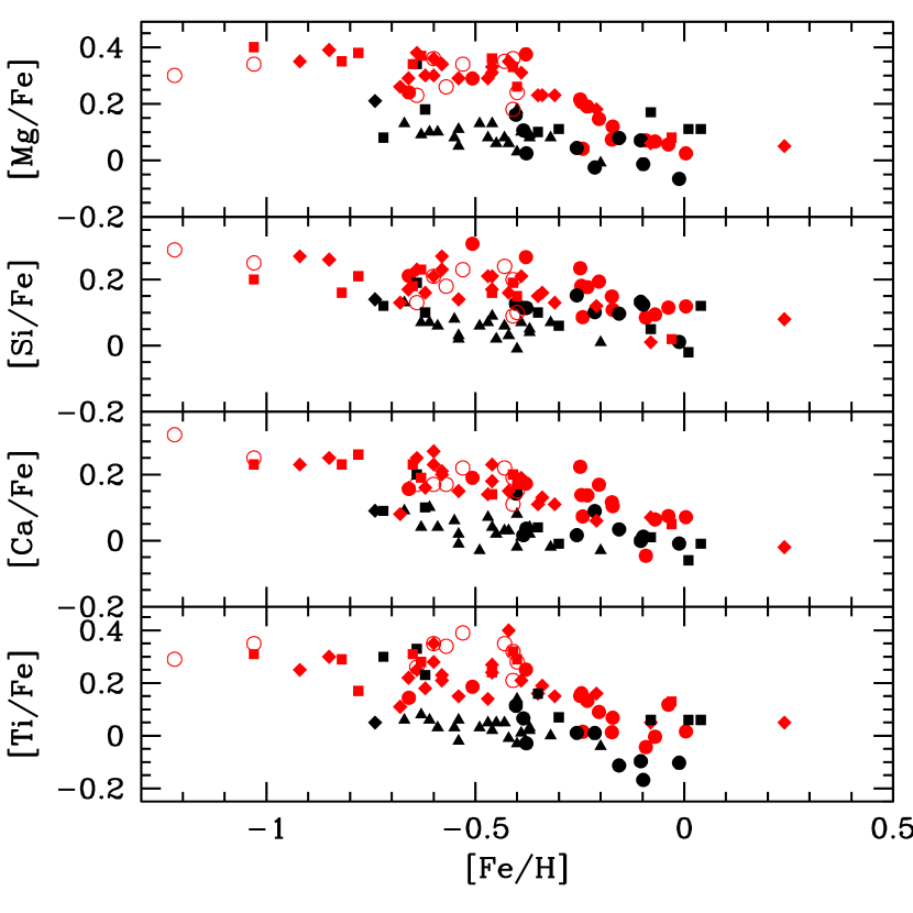
Figure 16: Comparison of O, Mg, Si, Ca, and Ti abundances with other studies. Red indicates thick disk stars; black thin disk stars. Our results are shown as filled circles; those from Prochaska et al. (2000) as open circles; Edvardsson et al. (1993) as filled squares; Bensby et al. (2003, 2004a) as filled diamonds; and Reddy et al. (2003) as filled triangles.

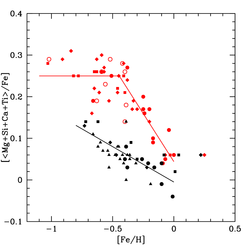
Figure 17: A comparison of average $\alpha$-element (Mg, Si, Ca, Ti) abundances with other studies. Same symbols as Figure 16. The sloped lines are linear least squares fits, as described in Section 8.1. For thick disk stars with [Fe/H] $\leq\ -0.4$, a straight mean for all stars has been shown.

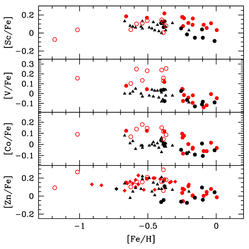
Figure 18: Comparison of Sc, V, Co, and Zn abundances with other studies. Same symbols as Figure 16.

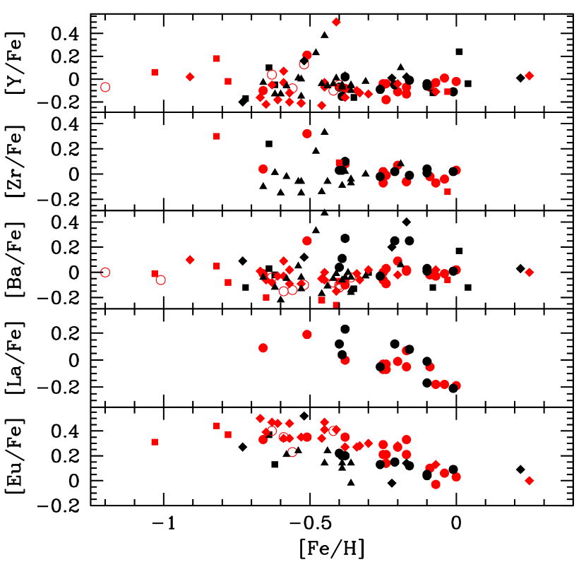
Figure 19: Comparison with other studies of heavy element abundances. Same symbols as Figure 16 with inverted filled triangles representing data from Mashonkina & Gehren (2000, 2001).

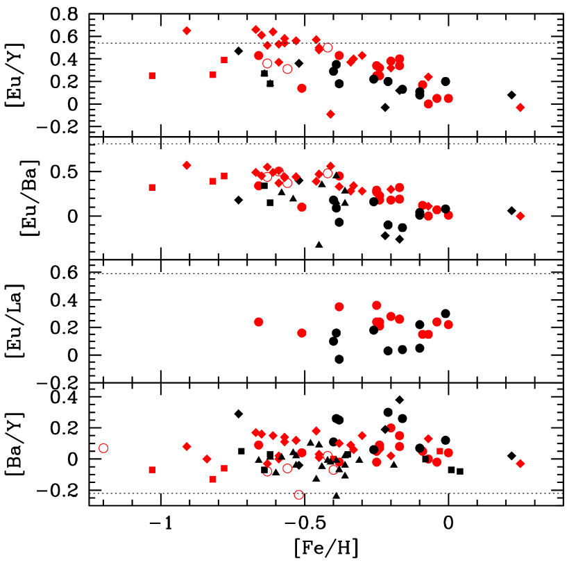
Figure 20: Comparison with other studies of $r$-process to $s$-process elemental abundance ratios. The symbols are the same as Figure 19. The dotted lines represent the predicted ratio for production of both elements only via the $r$-process, using results from Burris et al. (2000).

Note that BD+4 2696, at [Fe/H] = $-0.24$, does not follow the trend of the other thick disk stars, and that its abundance pattern is similar to the thin disk stars. We assume that our assignment of this star to the thick disk population, based on its kinematics, were inappropriate and that it represents a thin disk star whose kinematics put it in the high velocity tails of the thin disk velocity distributions. We have, nonetheless, shown the star as a thick disk star in Figures 10-16 and 18-20. For clarity, we have omitted the star from Figure 17. The star has [$\alpha$/Fe] = +0.05.

7.2 Al & Na

The odd-Z, light elements Al and Na are thought to be produced primarily in SNe II (Woosley & Weaver 1995) and, therefore, they should be enhanced in stars born during the earliest stages of star formation, presumably the stars with the lowest [Fe/H] values. Figure 11 shows that the behavior seen in the $\alpha$ elements is repeated in the case of aluminum, but not in sodium, as might have been expected. The thick disk stars show a plateau (at [Al/Fe] $\approx+0.3$) for [Fe/H] $<-0.3$, or, possibly a slow rise in [Al/Fe] as [Fe/H] decreases. The thin disk abundances remain near solar. The Al abundance of BD+4 2696 falls below the rest of the thick disk stars, just as it does for the $\alpha$-elements.

Unlike the $\alpha$-elements, Na abundances, shown in Figure 11, remain near solar over the entire metallicity range for both the thick and thin disk stars. Our Na abundances show no trend with metallicity for either the thick or thin disk, though the average thick disk abundance is slightly higher (0.04 dex) than that of the thin disk stars. This is quite surprising, and we have no explanation for the dissimilarity in the behavior of Na from Al.

7.3 Iron Peak Elements

The even-Z iron peak elements Ni and Cr follow Fe in both the thick and thin disk stars as can be seen in Figure 12. Unfortunately, the the abundances derived from ionized chromium lines are significantly higher than those obtained using neutral lines (by an average of 0.11 dex). Since significantly more neutral lines were measured, we have relied solely on [Cr I/Fe I] values to obtain the [Cr/Fe] abundance ratios. We do not understand the source of the disagreements between Cr I and Cr II abundances, but our first guess would be that the $gf$ values need to be re-determined.

Enhancements in [Sc/Fe] have been seen in metal-poor stars (Zhao & Magain 1990), and Nissen et al. (2000) suggested that Sc is produced in the same site as the $\alpha$-elements. Our results are consistent with this suggestion, in that [Sc/Fe] appears to behave similarly to the $\alpha$ elements, with higher abundances for the thick disk stars compared to the thin disk. Bensby et al. (2003) had noted the similarity in the behavior of [Zn/Fe] with the $\alpha$ elements, and we confirm that behavior, along with that of [Co/Fe] (Figure 13). For all three elements, BD+4 2696 continues to behave chemically like a thin disk star. We are unaware of any explanation as to why cobalt and zinc should show such behavior. Vanadium may also show this behavior but with a reduced amplitude, and the scatter in Figure 12 prohibits any firm conclusions.

The supernovae yields of Mn seem to be metallicity-dependent as studies of metal poor stars reveal underabundances of Mn at low metallicities (Gratton 1989, Reddy et al. 2003, Prochaska et al. 2000). We observe [Mn/Fe] to decrease with decreasing metallicity in both our thin and thick disk samples with no distinction between the two populations.

[Cu/Fe] in the thick disk is enhanced mildly for [Fe/H] $<-0.2$ at which point there appears to a small ($\approx$ 0.1 dex) step-like decrease to thin disk abundances. The thin disk stars all appear to have [Cu/Fe] abundance ratios at or slightly below the solar value.

7.4 Heavy Elements

The light neutron-capture elements Sr, Y, and Zr are thought to be significantly produced in the $weak$ $s$-process, which has been proposed to occur in advanced evolutionary phases of massive (M $>$ 10 M_⊙) stars (Lamb et al. 1977). Because these elements are produced in massive stars, they should be overabundant at early epochs, though because the $weak$ $s$-process elements’ production has been suggested to depend on metallicity (Raiteri et al. 1992), the overabundance may not be as great as that of the $r$-process elements.

Because the stars in this study are metal-rich, several of the most commonly used Sr II lines are saturated and heavily blended with Fe lines, making them unusable. This leaves one clean Sr I line and one fairly clean Sr II line. The Sr I lines gives consistently lower abundances (by $\approx$ 0.25 dex), than the Sr II line. Indeed, this is seen in our derived solar abundances (Table 9). Reddy et al. (2003) found similar behavior in that the Sr I line yielded [Sr/Fe] 0.35 dex too low in their solar analysis. Therefore, we cite results in Tables 10 and 11 and show abundances using only the Sr II line in Figure 14, though this line could not be measured in a few of the most metal-rich stars because of blending.

Figure 14 shows no difference between the thick disk and thin disk abundances of Sr, Y, and Zr. The thick disk star BD+47 2491, at [Fe/H] = $-0.51$, shows a significant enhancement in all $s$-process elements we measured. While this behavior could have been caused by mass transfer from a highly-evolved AGB companion, no sign of orbital motion is seen in our radial velocity monitoring (Table 1).

Ba, La, and Ce are thought to be formed during the $main$ $s$-process. The $main$ $s$-process accounts for the majority of the $s$-process abundances in elements with Z $\geq$ 56, and is thought to be occur primarily in low-mass (M $<$ 4 M_⊙) AGB stars during He-shell burning (Busso, Gallino, & Wasserburg 1999). In solar system material, Burris et al. (2000) estimated the $s$-process contributions to be 85%, 75%, and 81% for these three elements, respectively. Ba can be difficult to measure since its lines are often very strong and exhibit both hyperfine and isotopic splitting. Small changes in equivalent widths and microturbulent velocity may therefore result in differences in the derived abundances. Nonetheless, we find interesting differences between the thin disk and thick disk stars in the abundances of all three of these heavy $s$-process elements. Once again, BD+47 2491 is enhanced in these $s$-process elements. Neglecting that star, it is the thin disk stars that show enhanced abundance ratios in [Ba/Fe], [La/Fe], and [Ce/Fe], at least for [Fe/H] $<-0.2$. Again, it is clear that the chemical enrichment history of the thin disk has been quite different than that of the thick disk.

Nd is produced by both the $r$- and $s$-process, almost 50% by each process for solar system material (Burris et al. 2000). The abundances of this element therefore represent a mixture of the two processes. Figure 15 shows enhanced [Nd/Fe] ratios at lower [Fe/H] for both populations, but, as in the case of the other heavy $s$-process elements, Ba, La, and Ce, [Nd/Fe] is slightly enhanced in the thin disk stars compared to the thick disk stars for [Fe/H] $<-0.2$, and, hence, behaves more like an $s$-process element than one synthesized in the $r$-process.

Though the site of the $r$-process is not completely understood, it has been proposed to occur in SNe II (Wasserburg & Qian 2000). As the only $r$-process element we able to measure, Eu values play an important role in understanding the heavy element history of the thick and thin disks. (Its solar $r$-process contribution is estimated to be 91%, according to Burris et al. 2000.) The [Eu/Fe] results in Figure 15 show a similar pattern as the [$\alpha$/Fe] trends seen in Figure 10, which is consistent with also being produced in SNe II. The thick disk [Eu/Fe] ratio is $\approx$ +0.3 dex for [Fe/H]$<-0.2$, at which point there appears to be a step-like, or at least very steep, decrease to solar values. The thin disk [Eu/Fe] vs. [Fe/H] trend is smoother, declining steadily as [Fe/H] increases. Once again, BD+4 2696 behaves like a thin disk star in its [Eu/Fe] ratio.

8 COMPARISON WITH OTHER STUDIES

For a variety of reasons, we must compare our results with other disk abundance studies where stars from the thick and thin disk populations were chosen and analyzed in manners similar to those we have employed. For example, while others have found that [$\alpha$/Fe] vs. [Fe/H] trends differ for thin disk and thick disk stars, do Sc, Co, and Zn also obey these trends? Further, comparing with other results can help assess the comparability of our results, and combined samples have much greater power in addressing the key question about the origin of the thick disk population. In merging the samples, we have taken special care with three critical issues. First, we have relied on stars whose estimated ages are large, for reasons discussed earlier. We have also relied on kinematics, especially using probabilities of thin disk or thick disk membership. Finally, we have shifted all iron and element-to-iron results to the solar abundance scale we have adopted to reduce that source of systematic differences. We have not re-analyzed the work of others for possible differences in the treatment of isotopic or hyperfine splitting.

For the thick disk comparison, we use the abundances of our earlier work (Prochaska et al. 2000). That study used stars selected in the same manner as in this study: by kinematics and life expectancies. These should be the best comparison for our stars as we used the same $gf$ values as did they. We have also employed the thick disk stars identified and studied by Edvardsson et al. (1993) and by Bensby et al. (2003, 2004a, 2005). In all these cases, we relied on two primary criteria. First, the published estimates for the ages of the stars must equal or exceed 8 Gyrs. Second, the probability of thick disk membership, computed by Venn et al. (2004), must equal or exceed 80%. We note that Bensby et al. (2004b) found that those population assignments resulted in a very large mean age, although there might be a trend to somewhat lower ages at the higher metallicities.

To be considered as part of the thin disk, membership probability must equal or exceed 80%. We employed stars from the studies by Edvardsson et al. (1993), Bensby et al. (2003, 2004a, 2005), and Reddy et al. (2003). We believe that the best comparison between the thin and thick disk populations is with comparably old stars. We employed a slightly milder age criterion in order to provide a comparable sample of stars. Specifically, we included only those stars whose ages estimated by Edvardsson et al. (1993), Bensby et al. (2003), or Reddy et al. (2003) are at least 7 Gyrs. For the few stars without age estimates, we followed our own practice and retained stars only if their life expectancies exceed 10 Gyrs, following the same procedures described in Section 5.1.

We have excluded three “interlopers” from the comparisons. HD 78747 has a high probability of being a thin disk star according to Venn et al. (2004) but chemically it behaves like a thick disk star, with [$<$Mg+Si+Ca+Ti$>$/Fe] = +0.26 at [Fe/H] = $-0.64$. We have already drawn attention to BD+4 2696 in our own sample (see Section 7.1), and have excluded it. HD 4597 from Bensby et al. (2003) was assigned to the thick disk by Venn et al. (2004) yet shows thin disk chemical abundances ([$<$Mg+Si+Ca+Ti$>$/Fe] = +0.06 at [Fe/H] = $-0.34$. Given our probability selection limit for population assignments was $\geq 80$%, we are not surprised by a few interlopers. criterion, but again relied upon the population assignments from Venn et al. (2004).

We have supplemented the results for a subset of the stars studied by Edvardsson et al. (1993) with the Ba and Eu abundances obtained by Koch & Edvardsson (2002).

We have also employed results for the $s$-process and $r$-process elements from Mashonkina & Gehren (2000, 2001), following their population designations. These population assignments may differ in detail from those made by Venn et al. (2004).

8.1 Alpha Elements

We have not made direct comparisons between our results for [O/Fe] and those from other workers for reasons described earlier. Not only are non-LTE effects potentially important, but some workers do not include them (such as this paper), and others do attempt such corrections. Even so, the corrections are not always handled in the same manner, and it may be useful at a later time to merge all the data and undertake a comprehensive re-analysis of the data.

For Mg, Si, Ca, and Ti, careful inspection of Figure 16 shows good agreement between our results and those from Prochaska et al. (2000), as we would have expected given the similarity of the analytical methods and basic data, as well as those from the other studies. Of greater importance, however, is the confirmation of our finding that the $\alpha$-elements indicate a rather different nucleosynthesis history for the thick disk than for the thin disk. In general the $\alpha$-elements maintain a high value for the thick disk stars for [Fe/H] $\leq\ -0.4$, above which they decline toward solar values rather steeply. The thin disk stars show the same declines, but the slopes are shallower, and begin at a much lower metallicity. These trends are represented better in Figure 17, where we have averaged the behaviors of the four $\alpha$-elements measured in most of the dwarf and subgiant stars: Mg, Si, Ca, and Ti. Please note that here we have excluded BD+4 2696, which, as we have noted, does not appear to behave chemically like thick disk stars, despite its high probability of thick disk membership. The solid lines represent formal fits to the data. For the thin disk, the slope was computed using stars with $-0.8\leq$ [Fe/H] $\leq\ 0.0$. For the thick disk, a straight mean was calculated for the stars with $-1.1\leq$ [Fe/H] $\leq\ -0.4$, and a slope was computed for the stars with $-0.4\leq$ [Fe/H] $\leq\ 0.0$. The two stellar populations obviously show different trends.

8.2 Iron Peak Elements

We have already noted that some iron peak elements may behave similarly to the $\alpha$-elements, implying contributions to their abundances relative to iron from SNe II. In fact, Prochaska et al. (2000) had already drawn attention to the apparently high values of scandium, vanadium, cobalt, and zinc in most or all of the thick disk stars they analyzed.

In Figure 18 we show the behaviors of these four elements. We do not show results for Mn, Cr, Ni, and Cu since these elements show no statistical difference between the thick and thin disk populations. Our results agree well with those of Prochaska et al. (2000) and, in the case of zinc, with Bensby et al. (2003). For Sc, V, Co, and Zn, there are significant differences between the thin disk and thick disk populations.

8.3 Heavy Elements

In Figure 19 we show the results for the $s$-process elements Y, Zr, Ba, and La, and the $r$-process element, Eu. We have noted already that while BD+47 2491 behaves like other thick disk stars in [Eu/Fe], all of its $s$-process elements appear to be enhanced substantially.

Y and Zr are representative of the weak $s$-process, and [Y/Fe] and [Zr/Fe] are only slightly different between the thick and thin disk stars, although there is significant scatter among the various studies.

Barium is the most widely studied of the heavy $s$-process elements, and, like La, is produced in the main $s$-process. As seen in Figure 19, the thick disk has lower [Ba/Fe] ratios than does the thin disk, at least for [Fe/H] $<-$0.4. (We use the solar-corrected [Ba/Fe] results from Prochaska et al. 2000 since they agree much better with other results.) There is good agreement between studies for the thick disk abundances, and the scatter seen among the thick disk appears smaller than is seen among the thin disk stars. The lower [Ba/Fe] ratios seen in the thick disk agree with the idea that Ba production is from low-mass stars, and these low mass stars began contributing to the thick disk at a higher metallicity than did those enriching the thin disk. This is another indication of a high rate of star formation in the thick disk population. Unfortunately, we have not found any other studies of La in disk stars with which to compare our data.

The Eu abundances in Figure 19 show very good agreement between studies. The thick disk stars from Mashonkina & Gehren (2000, 2001), Prochaska et al. (2000), Bensby et al. (2005), and our study all show an enhancement of $\approx$0.4 dex for [Fe/H] $<-$0.4. This is perhaps not surprising given that the $\alpha$-elements are thought to be synthesized primarily in SNe II events, as are the $r$-process elements.

In Figure 20 we present these results in an alternative manner, following oft-used ratios that reflect the $r$-process element Eu and the $s$-process elements Y, Ba, and La, and plotted in such a way that we anticipate high values when SNe II are the dominant sources of nucleosynthesis contributions. We note that La has fewer potential problems than does Ba in the abundance determinations since the La lines are weaker, and form deeper in the stellar atmospheres, where non-LTE effects are less likely to introduce systematic errors.

If the light $s$-process element Y is created in 10 $M_{\odot}$ stars (the weak $s$-process), [Eu/Y] should have a roughly constant ratio, since Eu is likewise thought to be created in the deaths of (even more) massive stars. While the scatter is large, this expectation is borne out for the thick disk stars. The thin disk stars, however, show a decline from [Eu/Y] $\approx+0.2$ to 0.0 as [Fe/H] rises from $-0.8$ to $-0.5$. The thick disk stars maintain a high [Eu/Y] ration until [Fe/H] $\approx\ -0.2$, at which point there appears to be a sharp decrease to solar values, reminiscent of the behavior of [Cu/Fe].

Since the main $s$-process occurs on a much longer timescale than the $r$-process, [Eu/Ba] is expected to be enhanced early in a population’s star formation history. Figure 20 shows the [Eu/Ba] abundances, with the pure $r$-process abundance ratio (Burris et al. 2002) shown by a dotted line. The scatter in the [Eu/Ba] abundance ratios is unfortunately rather large, but it is clear that the thick disk stars show a larger enhancement of the $r$-process, at least as represented by europium, than does the thin disk. Indeed, comparison of Figure 20 with Figure 17 shows very similar trends. The thick disk stars show enhancement in [Eu/Fe] of $\approx$ 0.45 dex for $-0.7\leq$ [Fe/H] $<-$0.4. At [Fe/H] $\approx-$0.4, the [Eu/Ba] values for the thick disk stars begin to decrease, though they are still higher than the thin disk values up to [Fe/H] $\approx-$0.2. Combined with the $\alpha$-element abundances, this suggests that the star formation timescale is 1 Gyr or longer for the thick disk, at least in terms of producing stars with with [Fe/H] as high as $\approx\ -0.2$, based on the theoretical time scale for SNe Ia to begin enriching the ISM is $\approx$ 1 Gyr (Matteucci & Recchi 2001). Unfortunately, we have too few [Eu/La] results from which to draw any firm conclusions.

The $main$ to $weak$ $s$-process production may be compared through [Ba/Y] abundances. If the two elements were created in AGB stars with significantly different masses, as has seen suggested, we might see some structure in the [Ba/Y] vs. [Fe/H] plane, for both the thin disk and thick disk populations. The scatter is unfortunately too large to enable us to draw any meaningful conclusions.

9 THE HISTORY OF THE THICK DISK

9.1 Arguments in Favor of an Independent Origin for the Thick Disk

We summarize here what we believe to be the key points regarding an independent origin for the thick disk and the implied accretion of its parent galaxy.

First, the thick disk stars, at least in the solar neighborhood, are old (see Figure 1 and the discussion in Section 1). Second, the thick disk appears to have the same mean metallicity, independent of distance from the plane. There is no vertical metallicity gradient (Carney et al. 1989; Gilmore et al. 1995). Third, the limited evidence appears to show that the thin and thick disk populations maintain distinctive [Fe/H] vs. angular momentum trends (Figure 2). Finally, our results (Figures 10-15) and those of others (Figures 16-20) clearly show that the chemical enrichment histories of the thin and thick disk stellar populations have been very different, with the most prominent signature being that star formation proceeded more rapidly in the thick disk, such that [Fe/H] had reached levels as high as [Fe/H] $\approx-0.4$ before contributions from SNe Ia became significant, whereas in the thin disk star formation was slower, and SNe Ia contributions began to appear when [Fe/H] $\approx-1.0$.

We concur with Venn et al. (2004) that the abundance patterns seen among the dwarf galaxies that have been studied cannot be reconciled with those seen in among the thick disk stars, even when attention is restricted to those galaxies that completed their star formation in one primary, if possibly prolonged, burst. We say “prolonged” because the low [$\alpha$/Fe] values suggest SNe Ia events were contributing to the pollution of the interstellar media of these galaxies even when the [Fe/H] levels were still very low. Indeed, the low mean metallicities of these galaxies suggests that they were unable to retain the bulk of their gas and did not evolve as “closed box” systems.

The thick disk, on the other hand, has a high mean metallicity. If the thick disk arose due to the accretion of a small galaxy by the Milky Way, $<$[Fe/H]$>\approx-0.5$ suggests a fairly massive parent galaxy, comparable in mass to the Magellanic Clouds (see Grebel, Gallagher, & Harbeck 2003 for a good discussion of the relationships between dwarf galaxies’ mean metallicities and luminosities.) Unfortunately, direct comparison with elemental abundances and abundance ratios in thick disk stars and stars in the Magellanic Clouds is compromised by the continued star formation in both Clouds, and in the bulk of the available analyses referring to stars with younger ages. We would be caught in the same problems to which we have referred before were we to attempt such comparisons.

9.2 What Was the Progenitor Galaxy for the Thick Disk?

There are three remaining questions we may ask nonetheless.

First, what type of galaxy might have converted most of its gas into stars rapidly, so that we could see a behavior from its remnants within the Milky Way consistent with Figure 1? The answer does not appear to involve dwarf galaxies like the Magellanic Clouds nor the dwarf spheroidal galaxies. But it could have been a more compact dwarf elliptical galaxy.

Second, what is known about the abundance patterns in dwarf elliptical galaxies? Unfortunately, not very much, given their large distances. M32 is an interesting test case, and the literature is full of contradictory claims about the mean age and mean metallicity of its central regions, as well as about the bulk of its stellar population. The situation is finally becoming clearer (Schiavon, Caldwell, & Rose 2004; Rose et al. 2004; Worthey 2004). In the core of the galaxy, $<$[Fe/H]$>$ is higher than solar, and [Mg/Fe] is subsolar. From a chemical evolution perspective, this suggests that the core of M32 had a prolonged star formation history, enabling SNe Ia to contribute very significantly to the chemical enrichment. Schiavon et al. (2004), in fact, argue that the luminosity-weighted age of the stars in the core of M32 is only a few Gyrs, consistent with this view. The situation changes outside the core, with $<$[Fe/H]$>$ declining to $\approx-0.25$ at one effective radius. The weighted age rises as well, by about 3 Gyrs, although that remains very young in comparison to the age of the Galaxy’s thick disk stellar population. As would be expected, [Mg/Fe] is somewhat higher at one effective radius, roughly $-0.1$ compared to $-0.25$ in the core, but it remains subsolar and consistent with prolonged star formation. We conclude that M32, in its present state, is, like the other surviving dwarf galaxies, not a good template for the progenitor of the Galactic thick disk, although it is possible that had it merged with the Milky Way very early in its chemical evolution, it might have resulted in what we see today. We cannot distinguish the detailed chemical enrichment history of M32, unfortunately.

Third, what lessons may we learn from the wealth of elemental abundance ratios we and our colleagues have determined from careful studies of thick disk stars? There appear to be several answers, although not all are as firmly established as we desire.

• The “traditional” $\alpha$-elements O, Mg, Ca, and Si are enhanced relative to iron, for thick disk stars from [Fe/H] values as high as $-0.4$, at which point the abundance ratios begin to decline toward solar values. This can be understood, as we have stressed, if those elements arise in the rapid evolution of massive stars, and that such stars were able to enrich the interstellar medium of the thick disk’s progenitor galaxy much more rapidly than did the thin disk. SNe Ia begin to appear in the thin disk when [Fe/H] $\approx-1.0$ while the thick disk was able to reach [Fe/H $\approx-0.4$.

• Apparently other elements in the thick disk stars were also created primarily in rapidly-evolving massive stars, including Ti, Sc, V, Co, Zn, and Eu. The latter element’s comparable behavior is not at all surprising since in the solar system it is thought to have been created primarily in the $r$-process.

• The uniformity of the [Ba/Y] ratio in thick disk stars, and its similarity to values in seen among thin disk stars, at least for [Fe/H] $<-0.3$, suggests that only one of the two processes, the weak or the main $s$-process, were working. Perhaps neither $s$-process was working: ytrrium and barium both have contributions from the $r$-process. Qualitatively, we would expect enhanced [Eu/Y] and enhanced [Eu/Ba] ratios, as seen in Figure 20. Qantitatively, however, the actual ratios appear to fall short of “pure” $r$-process predictions. And it is also possible, even likely, that we have too few data, and that the scatter is too large, to discern the appearance or change in the relative contributions of the two $s$-processes.

• There is almost a “step function” or at least a very steep slope signifying rapid changes in the abundances of [Eu/Y] and [Eu/Fe], beginning at [Fe/H] $\approx-0.2$. Either a new nucleosynthesis source began to appear in the thick disk interstellar medium, or, possibly, its interstellar medium was being diluted by that of the Galactic thin disk. This could be a signal of the merger event itself.

9.3 Hierarchical Assembly of the Milky Way

In the above discussions we have assumed that the progenitor of the thick disk was a separate galaxy, which underwent its own star formation history, and which subsequently was captured and absorbed by the Milky Way, as opposed to the idea that the disk itself has experienced rather distinct episodes of star formation, for reasons that are not well understood. There is, perhaps, an attractive alternative that blends aspects of both metaphors. In essence, if galaxies are assembled in a hierarchical fashion, such that small units merge to make larger ones, out of which eventually emerge the galaxies we see today, the thick disk might have resulted from a merger of a moderately large such galaxy, but at an early time in the formation of the Milky Way itself. The thick disk progenitor would have still experienced a different chemical enrichment history, although perhaps not for very long. Brook et al. (2004, 2005) have developed chemodynamical evolutionary models that explain the observed features of the thick disk vs. the thin disk, including the differences in kinematics as well as [$\alpha$/Fe] vs. [Fe/H]. We certainly look forward to even more detailed models that explore as well the heavy $s$-process and $r$-process elements.

10 SUMMARY

We conclude that the thick disk does appear to have undergone a chemical enrichment history that was separate from that of the thin disk, most probably in a nearby dwarf galaxy. The star formation history was, however, sufficiently prolonged that SNe Ia were contributing to the galaxy’s interstellar medium by the time that the mean metallicity level had reached [Fe/H] = $-0.4$ (or, alternatively, [$\alpha$/H] $\approx-0.1$), where we now we could include Sc, V, Co, Zn, and Eu in this broad mix as elements created in the same mass range of stars, albeit in different sites, as the more “traditional” $\alpha$-elements. When $<$[Fe/H]$>$ in the thick disk parent galaxy reached $\approx-0.2$, however, its stars and gas appear to have merged with the Milky Way.

We are very grateful to the National Science Foundation for support through grants AST-9988156 and AST-030541 to the University of North Carolina. We also thank the anonymous referee for a challenging but ultimately very constructive review that improved this paper considerably.

Table 1: Radial Velocities

Name	N	Span	$V_{\rm rad}$	$\sigma$	E	I	E/I	P($\chi^{2}$)
BD+65 3	5	802	$-60.3$	0.2	0.2	0.4	0.7	0.776245
BD+69 238	5	1363	$-13.4$	0.2	0.4	0.4	1.0	0.393702
BD+34 927	12	3050	39.0	0.2	0.3	0.6	0.6	0.949663
BD+17 1145	12	3021	5.0	0.2	0.7	0.5	1.3	0.151076
BD+01 1600	7	2289	$-8.1$	0.2	0.4	0.5	0.9	0.489412
BD+30 1423	4	791	20.0	0.2	0.4	0.4	0.8	0.554606
BD+05 1611	8	2341	21.7	0.2	0.6	0.6	1.0	0.337620
BD+13 1655	4	791	38.5	0.2	0.4	0.4	0.9	0.447799
BD+46 1590	20	2547	33.7	0.1	3.9	0.5	7.2	0.000000
BD+06 2398	31	7316	19.0	0.1	0.7	0.5	1.4	0.000001
BD+18 2542	28	1838	15.4	0.3	3.1	0.7	4.8	0.000000
BD+11 2439	9	3166	$-24.6$	0.1	0.3	0.4	0.7	0.867265
BD+02 2585	18	3186	2.1	0.2	0.7	0.6	1.2	0.311593
BD+04 2696	7	3635	$-56.5$	0.3	0.6	0.7	0.9	0.461471
BD+09 2736	11	3186	$-7.0$	0.2	0.6	0.6	1.0	0.443047
BD+15 2658	41	3679	8.3	0.1	22.5	0.5	47.1	0.000000
BD+23 2747	11	2197	$-26.9$	0.1	0.4	0.4	0.9	0.649191
BD+26 2677	50	3665	$-29.8$	0.1	0.7	0.5	1.5	0.000000
BD+47 2491	9	2521	$-84.2$	0.2	0.4	0.5	0.9	0.534524
BD+45 2684	9	2015	$-64.9$	0.2	0.5	0.4	1.3	0.112319
BD+15 4026	8	2013	20.0	0.2	0.4	0.4	0.9	0.679412
BD+43 4116	11	2447	4.9	0.2	0.5	0.5	1.1	0.087191
BD+40 4912	9	2419	$-70.7$	0.2	0.4	0.4	1.0	0.450598

Table 2: Photometric Data

BD	HD	$V$	$b-y$	$m_{1}$	$c_{1}$	$\beta$	$K$	$J-K$	$V-K$
BD+65 3	404	8.62	0.516	0.425	0.326	$\cdots$	6.52	0.51	2.10
BD+69 238	25665	7.70	0.541	0.497	0.238	$\cdots$	5.46	0.53	2.24
BD+34 927	31501	8.16	0.453	0.257	0.303	2.554	6.30	0.44	1.86
BD+17 1145	42160	8.48	0.417	0.205	0.309	2.584	6.88	0.36	1.60
BD+1 1600	51219	7.40	0.431	0.236	0.326	2.599	5.72	0.43	1.68
BD+30 1423	53927	8.32	0.522	0.417	0.264	2.544	6.06	0.59	2.26
BD+5 1611	56202	8.42	0.400	0.187	0.318	2.609	6.93	0.32	1.49
BD+13 1655	57901	8.18	0.556	0.530	0.285	2.532	5.89	0.57	2.29
BD+46 1590	87899	8.88	0.423	0.193	0.259	$\cdots$	7.21	0.38	1.60
BD+6 2398	95980	8.25	0.402	0.199	0.338	2.592	6.72	0.37	1.53
BD+18 2542	103419	9.34	0.437	0.261	0.298	2.598	7.57	0.42	1.77
BD+11 2439	106210	7.57	0.421	0.206	0.327	2.587	5.94	0.40	1.63
BD+2 2585	111515	8.12	0.435	0.205	0.247	2.558	6.36	0.45	1.76
BD+4 2696	114094	9.67	0.434	0.229	0.278	2.562	8.02	0.42	1.65
BD+9 2736	115231	8.42	0.423	0.210	0.319	2.581	6.80	0.40	1.62
BD+15 2658	122676	7.13	0.458	0.242	0.314	$\cdots$	5.25	0.47	1.88
BD+23 2747	131042	7.50	0.411	0.188	0.309	2.577	5.90	0.33	1.60
BD+26 2677	136274	7.99	0.458	0.264	0.289	$\cdots$	6.12	0.41	1.87
BD+47 2491	159062	7.22	0.458	0.258	0.238	$\cdots$	5.39	0.41	1.83
BD+45 2684	168009	6.30	0.410	0.203	0.344	2.597	4.76	0.36	1.54
BD+15 4026	190067	7.15	0.452	0.233	0.287	$\cdots$	5.32	0.45	1.83
BD+43 4116	209393	7.97	0.417	0.234	0.262	2.581	6.32	0.39	1.65
BD+40 4912	215942	8.05	0.411	0.203	0.329	2.587	6.44	0.38	1.61

Table 3: Photometric Temperatures & Kinematics

Name	[Fe/H]phot	$T_{\rm eff}$	$T_{\rm eff}$	U	V	W	Thin	Thick
		($b-y$)	($V-K$)	km s-1	km s-1	km s-1	(%)	(%)
BD+65 0003	$-$0.09	5045	5005	$-$30	$-$42	2	0.48	0.51
BD+34 0927	$-$0.23	5348	5250	44	$-$48	43	0.09	0.88
BD+17 1145	$-$0.23	5542	5573	$-$19	$-$48	20	0.31	0.67
BD+01 1600	$-$0.03	5505	5484	$-$57	$-$46	$-$34	0.15	0.82
BD+13 1655	$-$0.17	4820	4800	6	$-$47	3	0.42	0.57
BD+04 2696	$-$0.26	5439	5500	71	$-$36	$-$45	0.11	0.90
BD+11 2439	$-$0.23	5532	5529	$-$58	$-$54	$-$42	0.05	0.90
BD+02 2585	$-$0.63	5366	5371	$-$50	$-$69	$-$35	0.03	0.92
BD+09 2736	$-$0.19	5527	5550	48	$-$60	0	0.17	0.81
BD+23 2747	$-$0.31	5583	5574	35	$-$45	13	0.38	0.60
BD+26 2677	$-$0.21	5301	5241	29	$-$61	23	0.12	0.85
BD+47 2491	$-$0.50	5259	5280	17	$-$44	$-$48	0.09	0.88
BD+45 2684	$-$0.11	5630	5631	$-$5	$-$46	$-$18	0.37	0.62
BD+40 4912	$-$0.12	5618	5554	$-$58	$-$50	13	0.24	0.73
BD+69 0238	$-$0.29	4855	4840	$-$4	$-$6	$-$13	0.84	0.16
BD+30 1423	$-$0.30	4959	4820	13	$-$11	$-$11	0.82	0.18
BD+05 1611	$-$0.26	5654	5731	61	$-$2	1	0.81	0.19
BD+46 1590	$-$0.52	5466	5476	37	5	16	0.84	0.15
BD+06 2398	$-$0.08	5674	5664	64	$-$7	$-$2	0.77	0.22
BD+18 2542	$-$0.03	5450	5358	16	13	20	0.86	0.13
BD+15 2658	$-$0.19	5331	5232	$-$8	11	17	0.87	0.12
BD+15 4026	$-$0.32	5335	5279	$-$63	$-$1	$-$11	0.79	0.21
BD+43 4116	$-$0.20	5537	5503	$-$4	20	8	0.91	0.09

Table 4: Observations

Date	Telescope	$\lambda$ range (Å)
January 14$-$19, 2000	KPNO	5000-7400
July 9$-$13, 2001	KPNO	3900-5500
January 28$-$31, 2002	KPNO	3700-5200
May 25$-30$, 2002	KPNO	3750-5300
July 25$-$29, 2002	KPNO	5420-7840
November 28$-$December 1, 2002	McDonald	3700-8600
January 12$-$14, 2003	McDonald	3800-8700

Table 5: Observational Data

Name	R. A.	DEC.	$V$	Red	Exp	S/N	Blue	Exp	S/N
	(J2000)	(J2000)		Date	(min)		Date	(min)
BD+65 0003	00 08 56.90	+65 38 47.0	8.61	01/2000	30	240	07/2001	65	135
BD+34 0927	04 57 59.37	+34 16 04.9	8.16	01/2000	35	410	11/2002	60	120
BD+17 1145	06 10 01.07	+17 56 03.2	8.48	01/2000	30	380	11/2002	60	150
BD+01 1600	06 56 34.19	+01 09 43.5	7.39	01/2000	10	280	11/2002	20	130
BD+13 1655	07 23 47.07	+12 57 53.0	8.18	01/2000	15	220	01/2002	30	120
BD+04 2696	13 08 13.16	+03 46 36.6	9.67	01/2000	30	210	05/2002	60	140
BD+11 2439	12 13 13.12	+10 49 18.0	7.57	01/2000	15	420	05/2002	20	250
BD+02 2585	12 49 44.83	+01 11 16.9	8.11	05/2003	30	490	01/2003	30	180
BD+09 2736	13 15 36.97	+09 00 57.7	8.42	01/2000	20	280	05/2002	40	210
BD+23 2747	14 50 40.98	+22 54 27.4	7.50	01/2000	10	300	01/2002	15	115
BD+26 2677	15 18 59.06	+25 41 30.1	7.99	01/2000	15	350	05/2002	20	170
BD+47 2491	17 30 16.43	+47 24 07.9	7.22	07/2002	10	400	05/2002	40	280
BD+45 2684	18 15 59.06	+45 12 33.5	6.31	07/2002	10	650	07/2001	30	255
BD+40 4912	22 48 13.95	+41 31 57.0	8.05	01/2000	27	240	07/2001	75	165
BD+69 0238	04 09 35.04	+69 32 29.0	7.70	01/2000	15	330	11/2002	60	100
BD+30 1423	07 08 04.24	+29 50 04.2	8.32	01/2000	40	230	11/2002	40	150
BD+05 1611	07 16 18.55	+05 04 33.9	8.41	01/2000	40	250	11/2002	30	190
BD+46 1590	10 09 14.20	+46 17 02.3	8.88	05/2003	10	200	01/2003	60	120
							01/2002	30	100
BD+06 2398	11 04 18.93	+05 47 44.5	8.25	05/2003	10	280	01/2003	60	180
							01/2002	15	130
BD+18 2542	11 54 33.78	+17 52 50.0	9.34	05/2000	90	250	05/2002	80	130
BD+15 2658	14 02 56.86	+14 58 31.2	7.13	01/2000	15	410	07/2001	25	115
BD+15 4026	20 02 34.12	+15 35 31.5	7.15	07/2002	10	400	05/2002	20	180
BD+43 4116	22 02 05.39	+44 20 35.4	7.97	07/2002	25	480	05/2002	20	240

Table 6: Atmospheric Parameters

Star	$T_{\rm eff}$	[M/H]	$\xi$(km/s)	log g	[FeI/H]	N	$\sigma$	[FeII/H]	N	$\sigma$
BD+65 3	5070	0.0	1.07	4.40	0.004	39	0.107	0.012	10	0.105
BD+34 927	5310	$-$0.4	1.00	4.60	$-$0.379	78	0.089	$-$0.375	14	0.097
BD+17 1145	5650	$-$0.2	1.03	4.40	$-$0.232	85	0.085	$-$0.237	19	0.075
BD+01 1600	5510	$-$0.1	1.13	4.30	$-$0.092	73	0.080	$-$0.096	17	0.094
BD+13 1655	4900	0.0	1.07	4.50	$-$0.038	43	0.090	$-$0.047	11	0.050
BD+04 2696	5520	$-$0.3	1.15	4.45	$-$0.243	75	0.087	$-$0.247	17	0.075
BD+11 2439	5600	$-$0.2	1.10	4.35	$-$0.204	62	0.081	$-$0.198	17	0.094
BD+02 2585	5380	$-$0.7	0.95	4.50	$-$0.659	103	0.072	$-$0.664	24	0.072
BD+09 2736	5610	$-$0.2	1.27	4.40	$-$0.171	72	0.086	$-$0.172	14	0.088
BD+23 2747	5680	$-$0.2	1.13	4.35	$-$0.173	70	0.073	$-$0.173	15	0.064
BD+26 2677	5400	$-$0.3	1.10	4.50	$-$0.246	65	0.089	$-$0.254	14	0.090
BD+47 2491	5260	$-$0.5	1.05	4.45	$-$0.507	68	0.095	$-$0.500	14	0.095
BD+45 2684	5720	$-$0.1	1.15	4.20	$-$0.070	70	0.078	$-$0.060	15	0.038
BD+40 4912	5620	$-$0.3	1.10	4.30	$-$0.249	74	0.082	$-$0.257	14	0.081
BD+69 238	4870	0.0	0.85	4.40	$-$0.012	73	0.099	$-$0.016	13	0.081
BD+30 1423	4960	$-$0.4	0.90	4.60	$-$0.385	78	0.094	$-$0.390	17	0.079
BD+05 1611	5720	$-$0.2	1.35	4.45	$-$0.156	69	0.073	$-$0.159	17	0.087
BD+46 1590	5520	$-$0.4	1.03	4.50	$-$0.378	120	0.082	$-$0.385	25	0.076
BD+06 2398	5680	$-$0.1	1.12	4.25	$-$0.104	119	0.089	$-$0.098	25	0.088
BD+18 2542	5420	$-$0.3	1.30	4.40	$-$0.257	69	0.099	$-$0.256	13	0.076
BD+15 2658	5450	$-$0.1	1.02	4.30	$-$0.098	67	0.072	$-$0.090	12	0.053
BD+15 4026	5410	$-$0.4	1.15	4.60	$-$0.403	76	0.089	$-$0.403	17	0.079
BD+43 4116	5620	$-$0.2	1.30	4.55	$-$0.214	78	0.091	$-$0.217	13	0.077

Table 7: Equivalent Widths for Thin Disk Stars

$\lambda$(Å)	$\chi$(eV)	log $gf$	ref	BD+69 238	BD+30 1423	BD+5 1611	BD+46 1590	BD+6 2398
					O I
7771.954	9.14	0.360	62	$\cdots$	$\cdots$	$\cdots$	44.5	$\cdots$
7774.177	9.14	0.210	62	$\cdots$	$\cdots$	$\cdots$	36.8	$\cdots$
7775.395	9.14	$-0.010$	62	11.9	11.4	43.2	28.8	$\cdots$
					Na I
5682.65	2.10	$-0.890$	99	149.9	122.1	89.6	77.9	92.9
5688.210	2.10	$-0.580$	99	$\cdots$	$\cdots$	112.1	110.8	114.1
6154.230	2.10	$-1.570$	48	77.9	51.6	30.2	25.6	40.1
6160.753	2.10	$-1.270$	48	94.7	70.7	41.2	37.8	57.1

Table 8: Uncertainties in Atmospheric Parameters

Ion	$\Delta\xi$	$\Delta\xi$	$\Delta T_{\rm eff}$	$\Delta T_{\rm eff}$	$\Delta$log g	$\Delta$log g	$\Delta$[M/H]	$\Delta$[M/H]
	+0.10	$-$0.10	+80K	$-$80K	+0.05	$-$0.05	+0.1	$-$0.1	$\sigma$
FeI/H	$-$0.022	0.024	0.042	$-$0.040	$-$0.003	0.005	0.016	$-$0.014	0.051
FeII/H	$-$0.016	0.022	$-$0.032	0.040	0.020	$-$0.018	0.035	$-$0.034	0.061
OI/Fe	0.012	$-$0.024	$-$0.158	0.146	0.013	$-$0.025	$-$0.016	0.004	0.163
NaI/Fe	0.022	$-$0.010	$-$0.003	0.006	$-$0.005	0.007	$-$0.009	0.011	0.026
MgI/Fe	0.018	$-$0.020	$-$0.026	0.022	$-$0.005	0.000	$-$0.008	0.002	0.034
AlI/Fe	0.022	$-$0.004	$-$0.014	0.026	0.003	0.005	$-$0.016	0.019	0.039
SiI/Fe	0.018	$-$0.016	$-$0.067	0.070	0.008	$-$0.005	0.004	$-$0.007	0.073
CaI/Fe	0.006	$-$0.008	0.005	$-$0.013	$-$0.014	0.009	$-$0.006	0.002	0.021
ScII/Fe	0.012	$-$0.008	$-$0.062	0.061	0.023	$-$0.023	0.017	$-$0.017	0.070
TiI/Fe	0.004	$-$0.006	0.034	$-$0.040	$-$0.001	0.000	$-$0.018	0.015	0.044
TiII/Fe	0.002	$-$0.006	$-$0.062	0.051	0.022	$-$0.026	0.015	$-$0.018	0.070
VI/Fe	0.014	$-$0.014	0.043	$-$0.051	0.000	$-$0.003	$-$0.020	0.017	0.057
CrI/Fe	0.001	0.002	0.024	$-$0.032	$-$0.007	0.004	$-$0.008	0.006	0.034
CrII/Fe	0.002	$-$0.004	$-$0.085	0.086	0.023	$-$0.021	0.010	$-$0.008	0.090
MnI/Fe	0.010	$-$0.008	0.016	$-$0.016	$-$0.002	0.002	$-$0.006	0.006	0.020
CoI/Fe	0.018	$-$0.022	$-$0.014	0.014	0.009	$-$0.012	$-$0.003	0.000	0.029
NiI/Fe	0.004	$-$0.006	$-$0.026	0.026	0.003	$-$0.005	0.005	$-$0.006	0.027
CuI/Fe	0.008	$-$0.012	$-$0.010	0.010	0.006	$-$0.009	0.004	$-$0.003	0.018
ZnI/Fe	$-$0.008	0.006	$-$0.070	0.073	0.013	$-$0.015	0.014	$-$0.016	0.077
SrI/Fe	$-$0.018	0.016	0.034	$-$0.038	$-$0.007	0.005	$-$0.016	0.014	0.046
SrII/Fe	0.008	$-$0.018	$-$0.078	0.074	0.023	$-$0.025	0.004	$-$0.016	0.085
YII/Fe	0.008	$-$0.010	$-$0.054	0.046	0.017	$-$0.022	0.019	$-$0.023	0.064
ZrII/Fe	0.002	$-$0.004	$-$0.046	0.050	0.023	$-$0.025	0.019	$-$0.016	0.059
BaII/Fe	$-$0.026	0.016	$-$0.042	0.030	0.010	$-$0.018	0.027	$-$0.033	0.062
LaII/Fe	0.022	$-$0.020	$-$0.042	0.042	0.023	$-$0.025	0.019	$-$0.016	0.057
CeII/Fe	0.014	$-$0.024	$-$0.046	0.038	0.023	$-$0.025	0.016	$-$0.020	0.061
NdII/Fe	0.018	$-$0.018	$-$0.037	0.038	0.024	$-$0.026	0.021	$-$0.018	0.054
EuII/Fe	0.012	$-$0.014	$-$0.043	0.034	0.020	$-$0.030	0.014	$-$0.019	0.058

Table 9: Derived Solar Abundances

Ion	log n⊙(X)	[X/H]	$\sigma$	N
Fe I	7.51	$-0.006$	0.067	91
Fe II	7.51	$-0.007$	0.081	22
O I	8.83	+0.036	$\cdots$	1
Na I	6.33	+0.004	0.017	4
Mg I	7.58	$-0.037$	0.080	4
Al I	6.47	$-0.021$	0.043	4
Si I	7.55	$+0.026$	0.035	10
Ca I	6.36	+0.013	0.060	14
Sc II	3.17	+0.008	0.032	6
Ti I	5.02	$-0.087$	0.061	49
Ti II	5.02	$-0.071$	0.092	15
V I	4.00	$-0.137$	0.053	16
Cr I	5.67	$-0.073$	0.065	17
Cr II	5.67	+0.090	0.058	5
Mn I	5.39	$-0.164$	0.071	15
Co I	4.92	$-0.032$	0.087	10
Ni I	6.25	+0.013	0.077	35
Cu I	4.21	$-0.003$	0.072	3
Zn I	4.60	$-0.074$	0.028	2
Sr I	2.97	$-0.260$	$\cdots$	1
Sr II	2.97	0.000	$\cdots$	1
Y II	2.24	$-0.070$	0.052	10
Zr II	2.60	$-0.029$	0.035	2
Ba II	2.13	+0.023	0.021	3
La II	1.17	$-0.069$	0.095	9
Ce II	1.58	$-0.018$	0.076	8
Nd II	1.50	$-0.054$	0.097	18
Eu II	0.51	+0.068	0.055	4

Table 10: Abundances - Thin Disk Stars

	BD+69			BD+30			BD+5			BD+46			BD+6
	238	$\sigma$	N	1423	$\sigma$	N	1611	$\sigma$	N	1590	$\sigma$	N	2398	$\sigma$	N
$[$O/Fe$]$	0.058	$\cdots$	1	0.260	$\cdots$	1	0.192	$\cdots$	1	0.214	0.010	3	0.160	0.017	3
$[$Na/Fe$]$	0.021	0.035	3	0.071	0.036	3	$-0.025$	0.057	4	0.014	0.055	4	0.080	0.034	4
$[$Mg/Fe$]$	$-0.066$	0.030	5	0.106	0.076	6	0.079	0.051	5	0.024	0.040	5	0.070	0.038	5
$[$Al/Fe$]$	$-0.027$	0.064	2	0.056	0.049	2	0.017	0.092	2	0.029	0.007	2	0.060	0.057	2
$[$Si/Fe$]$	0.011	0.048	9	0.114	0.047	12	0.097	0.032	11	0.114	0.049	11	0.204	0.062	13
$[$Ca/Fe$]$	$-0.009$	0.070	8	0.016	0.066	14	0.034	0.083	17	0.036	0.083	18	$-0.001$	0.075	18
$[$Sc/Fe$]$	$-0.089$	0.075	8	0.065	0.076	9	$-0.053$	0.060	8	0.129	0.084	10	0.039	0.065	10
$[$TiI/Fe$]$	$-0.103$	0.107	46	0.066	0.098	42	$-0.113$	0.082	40	$-0.029$	0.091	56	$-0.097$	0.070	56
$[$TiII/Fe$]$	$-0.125$	0.077	12	0.012	0.054	13	$-0.019$	0.071	12	0.081	0.082	20	0.012	0.091	19
$[$V/Fe$]$	$-0.090$	0.102	16	0.039	0.087	15	$-0.130$	0.090	16	$-0.076$	0.090	18	$-0.110$	0.077	18
$[$CrI/Fe$]$	$-0.040$	0.120	12	0.004	0.102	15	0.016	0.084	18	0.047	0.092	19	0.081	0.090	20
$[$CrII/Fe$]$	0.084	0.059	5	0.055	0.081	5	0.204	0.055	5	0.164	0.026	5	0.120	0.061	4
$[$Mn/Fe$]$	$-0.173$	0.072	10	$-0.180$	0.120	13	$-0.181$	0.082	15	$-0.123$	0.064	16	$-0.033$	0.075	15
$[$FeI/H$]$	$-0.012$	0.099	73	$-0.385$	0.094	74	$-0.156$	0.073	69	$-0.378$	0.082	120	$-0.104$	0.089	113
$[$FeII/H$]$	$-0.016$	0.081	13	$-0.390$	0.079	17	$-0.159$	0.087	17	$-0.385$	0.076	25	$-0.098$	0.088	25
$[$Co/Fe$]$	$-0.053$	0.040	10	0.010	0.069	10	$-0.092$	0.079	11	$-0.103$	0.089	11	0.008	0.070	12
$[$Ni/Fe$]$	0.022	0.081	34	0.034	0.093	38	$-0.019$	0.094	38	0.019	0.077	37	0.084	0.086	28
$[$Cu/Fe$]$	$-0.023$	0.049	2	0.005	0.071	2	$-0.157$	0.059	3	$-0.119$	0.010	4	0.006	0.054	4
$[$Zn/Fe$]$	0.043	0.035	2	$-0.044$	0.021	2	$-0.018$	0.014	2	0.109	0.021	2	0.095	0.007	2
$[$SrII/Fe$]$	0.002	$\cdots$	1	0.195	$\cdots$	1	0.206	$\cdots$	1	0.078	$\cdots$	1	0.054	$\cdots$	1
$[$Y/Fe$]$	$-0.112$	0.078	8	$-0.149$	0.082	6	$-0.007$	0.062	8	0.021	0.059	10	$-0.042$	0.065	10
$[$Zr/Fe$]$	0.018	0.060	2	0.026	0.064	2	$-0.008$	0.028	2	0.104	0.028	2	0.040	0.028	2
$[$Ba/Fe$]$	0.012	0.060	3	0.105	0.056	3	0.253	0.032	3	0.268	0.020	3	0.031	0.023	3
$[$La/Fe$]$	$-0.209$	0.073	9	0.037	0.112	9	0.076	0.072	9	0.229	0.073	9	$-0.013$	0.094	9
$[$Ce/Fe$]$	0.041	0.088	10	0.160	0.090	7	0.086	0.094	8	0.043	0.054	10	0.070	0.086	10
$[$Nd/Fe$]$	$-0.155$	0.097	9	0.103	0.095	10	0.140	0.083	9	0.260	0.097	14	$-0.033$	0.095	14
$[$Eu/Fe$]$	0.092	0.039	4	0.198	0.049	4	0.124	0.056	4	0.201	0.052	4	0.042	0.043	4

Table 10: Abundances - Thin Disk Stars

	BD+18			BD+15			BD+15			BD+43
	2542	$\sigma$	N	2658	$\sigma$	N	4026	$\sigma$	N	4116	$\sigma$	N
$[$O/Fe$]$	$\cdots$	$\cdots$	$\cdots$	$\cdots$	$\cdots$	$\cdots$	0.132	0.057	3	0.150	0.046	3
$[$Na/Fe$]$	0.083	0.014	4	0.009	0.048	4	0.042	0.053	4	$-0.038$	0.051	4
$[$Mg/Fe$]$	0.043	0.056	4	$-0.014$	0.051	5	$-0.161$	0.048	5	$-0.026$	0.057	5
$[$Al/Fe$]$	0.103	$\cdots$	1	$-0.066$	0.014	2	0.154	0.049	2	$-0.030$	0.028	2
$[$Si/Fe$]$	0.152	0.059	11	0.124	0.036	11	0.127	0.045	11	0.101	0.055	11
$[$Ca/Fe$]$	0.016	0.060	14	0.012	0.082	18	0.142	0.073	16	0.089	0.080	16
$[$Sc/Fe$]$	0.051	0.083	9	$-0.053$	0.060	9	0.110	0.074	9	$-0.016$	0.089	8
$[$TiI/Fe$]$	0.011	0.098	41	$-0.168$	0.087	43	0.114	0.079	43	0.010	0.088	39
$[$TiII/Fe$]$	0.050	0.084	8	$-0.085$	0.078	11	0.090	0.088	14	0.077	0.098	14
$[$V/Fe$]$	0.026	0.101	15	$-0.083$	0.066	14	0.033	0.077	14	$-0.065$	0.086	15
$[$CrI/Fe$]$	0.009	0.071	16	$-0.038$	0.092	18	$-0.017$	0.069	19	0.004	0.066	19
$[$CrII/Fe$]$	0.217	0.091	5	0.104	0.057	5	0.059	0.064	5	0.106	0.067	5
$[$Mn/Fe$]$	$-0.082$	0.079	13	$-0.143$	0.094	14	$-0.155$	0.056	13	$-0.132$	0.089	13
$[$FeI/H$]$	$-0.257$	0.099	69	$-0.098$	0.072	67	$-0.403$	0.089	76	$-0.214$	0.091	78
$[$FeII/H$]$	$-0.256$	0.076	13	$-0.090$	0.053	12	$-0.403$	0.079	17	$-0.217$	0.077	13
$[$Co/Fe$]$	$-0.049$	0.072	8	$-0.104$	0.064	10	0.036	0.070	11	$-0.080$	0.089	10
$[$Ni/Fe$]$	$-0.023$	0.099	33	0.020	0.082	35	$-0.011$	0.082	35	$-0.106$	0.092	37
$[$Cu/Fe$]$	$-0.020$	0.081	3	$-0.025$	0.075	3	$-0.002$	0.058	4	$-0.166$	0.053	4
$[$Zn/Fe$]$	$-0.062$	0.035	2	$-0.041$	0.021	2	$-0.066$	0.021	2	$-0.075$	0.021	2
$[$SrII/Fe$]$	$-0.033$	$\cdots$	1	0.068	$\cdots$	1	$-0.017$	$\cdots$	1	0.074	$\cdots$	1
$[$Y/Fe$]$	$-0.094$	0.057	7	$-0.058$	0.067	9	$-0.069$	0.090	8	$-0.049$	0.075	8
$[$Zr/Fe$]$	$-0.022$	0.035	2	0.014	0.042	2	0.029	0.057	6	0.015	0.021	2
$[$Ba/Fe$]$	$-0.026$	0.060	3	0.011	0.021	3	0.036	0.035	3	0.247	0.064	3
$[$La/Fe$]$	$-0.051$	0.072	9	$-0.168$	0.104	9	0.103	0.082	9	0.121	0.085	9
$[$Ce/Fe$]$	$-0.020$	0.039	7	$-0.030$	0.042	7	0.136	0.07	8	0.169	0.079	9
$[$Nd/Fe$]$	$-0.110$	0.084	8	$-0.104$	0.089	9	0.153	0.103	11	0.172	0.081	10
$[$Eu/Fe$]$	0.130	0.050	4	0.051	0.069	4	0.223	0.047	4	0.154	0.054	4

Table 11: Abundances - Thick Disk Stars

	BD+65			BD+34			BD+17			BD+1			BD+13
	3	$\sigma$	N	927	$\sigma$	N	1145	$\sigma$	N	1600	$\sigma$	N	1655	$\sigma$	N
$[$O/Fe$]$	$\cdots$	$\cdots$	$\cdots$	0.475	0.061	3	0.318	0.057	2	0.048	0.078	2	$\cdots$	$\cdots$	$\cdots$
$[$Na/Fe$]$	0.082	0.021	2	0.075	0.037	4	0.090	0.031	4	0.043	0.054	4	0.109	0.035	2
$[$Mg/Fe$]$	0.024	0.053	4	0.375	0.058	6	0.190	0.092	6	0.070	0.033	5	0.056	0.055	5
$[$Al/Fe$]$	0.310	0.035	2	0.280	0.021	2	0.198	0.057	2	0.073	0.035	2	0.149	0.064	2
$[$Si/Fe$]$	0.131	0.065	8	0.268	0.053	12	0.177	0.033	12	0.176	0.042	10	0.215	0.066	11
$[$Ca/Fe$]$	0.071	0.063	8	0.172	0.075	15	0.137	0.065	17	$-0.046$	0.089	16	0.074	0.077	5
$[$Sc/Fe$]$	0.032	0.093	9	0.217	0.077	9	0.164	0.068	9	0.091	0.053	8	0.108	0.079	8
$[$TiI/Fe$]$	0.016	0.103	41	0.251	0.093	51	0.133	0.086	50	$-0.043$	0.092	53	0.118	0.083	30
$[$TiII/Fe$]$	$-$0.058	0.098	9	0.314	0.072	13	0.150	0.042	13	$-$0.051	0.082	14	0.039	0.105	8
$[$V/Fe$]$	$-0.047$	0.100	14	0.118	0.088	17	$-0.015$	0.062	16	$-0.140$	0.067	16	$-$0.005	0.107	14
$[$CrI/Fe$]$	$-0.047$	0.095	14	$-$0.002	0.076	17	0.049	0.076	19	$-$0.008	0.091	17	$-$0.024	0.088	11
$[$CrII/Fe$]$	0.160	0.074	4	0.193	0.058	5	0.110	0.059	5	0.110	0.068	5	0.116	0.057	5
$[$Mn/Fe$]$	$-$0.052	0.100	9	$-$0.240	0.091	16	$-0.108$	0.088	16	$-$0.119	0.082	14	$-$0.046	0.079	9
$[$FeI/H$]$	0.004	0.107	39	$-$0.379	0.089	78	$-$0.236	0.085	85	$-$0.092	0.080	73	$-$0.038	0.090	43
$[$FeII/H$]$	0.012	0.105	10	$-$0.375	0.097	14	$-$0.235	0.075	19	$-$0.096	0.094	17	$-$0.047	0.050	11
$[$Co/Fe$]$	$-$0.032	0.073	10	0.118	0.053	11	0.078	0.044	11	$-$0.060	0.053	11	0.015	0.068	10
$[$Ni/Fe$]$	0.027	0.103	31	0.038	0.095	38	0.065	0.083	38	$-$0.002	0.081	38	0.065	0.108	29
$[$Cu/Fe$]$	0.016	0.028	2	0.076	0.080	3	0.099	0.072	3	0.005	0.035	3	$-$0.010	0.028	2
$[$Zn/Fe$]$	$-$0.013	0.035	2	0.180	0.064	2	0.073	0.049	2	0.003	0.064	2	0.079	0.078	2
$[$SrII/Fe$]$	0.086	$\cdots$	1	$-0.171$	$\cdots$	1	0.012	$\cdots$	1	$-0.218$	$\cdots$	1	0.198	$\cdots$	1
$[$Y/Fe$]$	$-$0.024	0.085	7	$-$0.079	0.065	8	$-$0.040	0.052	9	$-$0.065	0.046	8	0.014	0.093	7
$[$Zr/Fe$]$	0.032	0.071	2	0.075	0.028	2	$-$0.012	0.057	2	$-$0.022	0.028	2	$-$0.036	0.057	2
$[$Ba/Fe$]$	0.016	0.044	3	$-$0.098	0.049	3	0.029	0.075	3	$-$0.048	0.052	3	$-$0.009	0.085	3
$[$La/Fe$]$	$-$0.187	0.094	8	0.002	0.112	9	$-$0.028	0.076	9	$-$0.094	0.094	9	$-$0.181	0.102	9
$[$Ce/Fe$]$	0.073	0.078	8	0.047	0.091	10	0.017	0.064	10	0.077	0.063	9	0.111	0.071	7
$[$Nd/Fe$]$	$-$0.172	0.123	7	0.054	0.087	12	0.020	0.092	11	$-$0.101	0.108	14	$-$0.005	0.126	9
$[$Eu/Fe$]$	0.031	0.026	4	0.347	0.068	4	0.206	0.043	4	0.103	0.050	4	0.060	0.046	3

Table 11: Abundances - Thick Disk Stars (continued)

	BD+4			BD+11			BD+2			BD+9			BD+23
	2696	$\sigma$	N	2439	$\sigma$	N	2585	$\sigma$	N	2736	$\sigma$	N	2747	$\sigma$	N
$[$O/Fe$]$	$\cdots$	$\cdots$	$\cdots$	$\cdots$	$\cdots$	$\cdots$	0.565	0.035	3	$\cdots$	$\cdots$	$\cdots$	$\cdots$	$\cdots$
$[$Na/Fe$]$	0.002	0.038	4	0.122	0.049	4	0.082	0.049	4	0.004	0.044	4	0.019	0.052	4
$[$Mg/Fe$]$	0.041	0.054	5	0.146	0.038	5	0.240	0.061	4	0.119	0.049	5	0.073	0.043	5
$[$Al/Fe$]$	$-0.021$	0.014	2	0.195	0.035	2	0.310	0.049	2	0.087	0.014	2	0.079	0.071	2
$[$Si/Fe$]$	0.086	0.041	10	0.194	0.049	11	0.211	0.055	14	0.108	0.044	11	0.149	0.053	14
$[$Ca/Fe$]$	0.073	0.069	16	0.169	0.056	16	0.156	0.057	17	0.104	0.058	16	0.116	0.062	17
$[$Sc/Fe$]$	0.076	0.076	9	0.111	0.086	9	0.185	0.066	10	0.161	0.077	9	0.091	0.047
$[$TiI/Fe$]$	0.015	0.093	43	0.090	0.080	42	0.144	0.065	57	0.068	0.097	50	0.013	0.071	39
$[$TiII/Fe$]$	0.045	0.075	13	0.165	0.063	13	0.231	0.059	20	0.160	0.066	14	0.152	0.076	12
$[$V/Fe$]$	$-0.075$	0.067	15	$-0.041$	0.077	14	0.079	0.085	18	$-0.018$	0.069	15	$-0.094$	0.084	15
$[$CrI/Fe$]$	0.058	0.097	18	0.079	0.086	20	0.046	0.080	18	0.014	0.083	17	0.005	0.076	20
$[$CrII/Fe$]$	0.065	0.009	5	0.128	0.051	5	0.135	0.031	5	0.069	0.019	5	0.137	0.068	5
$[$Mn/Fe$]$	$-0.182$	0.067	15	$-0.126$	0.041	15	$-0.159$	0.082	16	$-0.122$	0.073	15	$-0.200$	0.084	15
$[$FeI/H$]$	$-0.243$	0.087	75	$-0.204$	0.081	62	$-0.659$	0.072	103	$-0.171$	0.086	72	$-0.173$	0.073	70
$[$FeII/H$]$	$-0.243$	0.075	17	$-0.198$	0.094	17	$-0.664$	0.072	24	$-0.172$	0.088	14	$-0.172$	0.064	15
$[$Co/Fe$]$	$-0.083$	0.070	10	0.003	0.081	10	0.123	0.096	11	$-0.030$	0.058	11	$-0.039$	0.065	11
$[$Ni/Fe$]$	$-0.082$	0.094	35	0.030	0.091	35	0.059	0.082	38	$-0.025$	0.093	34	$-0.034$	0.072	35
$[$Cu/Fe$]$	$-0.107$	0.036	3	0.077	0.015	3	0.064	0.072	4	$-0.012$	0.055	3	0.096	0.080	3
$[$Zn/Fe$]$	$-0.056$	0.021	2	0.110	0.042	2	0.150	0.007	2	0.007	0.057	2	0.004	0.049	2
$[$SrII/Fe$]$	$-0.087$	$\cdots$	1	0.004	$\cdots$	1	$-0.161$	$\cdots$	1	0.111	$\cdots$	1	$-0.067$	$\cdots$	1
$[$Y/Fe$]$	$-0.184$	0.059	9	$-0.110$	0.034	8	$-0.098$	0.086	10	$-0.069$	0.058	9	$-0.125$	0.049	8
$[$Zr/Fe$]$	$-0.011$	0.000	2	0.065	0.007	2	0.035	0.028	2	$-0.063$	0.042	2	$-0.056$	0.021	2
$[$Ba/Fe$]$	$-0.090$	0.047	3	0.087	0.068	3	$-0.008$	0.021	3	0.011	0.044	3	0.023	0.044	3
$[$La/Fe$]$	$-0.069$	0.090	9	$-0.008$	0.073	9	0.086	0.101	9	0.065	0.060	9	$-0.049$	0.074	9
$[$Ce/Fe$]$	0.004	0.077	8	0.032	0.069	9	0.095	0.076	10	0.096	0.085	9	$-0.015$	0.071	7
$[$Nd/Fe$]$	$-0.119$	0.080	11	0.035	0.092	13	0.109	0.121	10	$-0.005$	0.092	13	$-0.081$	0.076	9
$[$Eu/Fe$]$	0.143	0.055	4	0.274	0.036	4	0.329	0.055	4	0.334	0.022	4	0.208	0.047	4

Table 11: Abundances - Thick Disk Stars (continued)

	BD+26			BD+47			BD+45			BD+40
	2677	$\sigma$	N	2491	$\sigma$	N	2684	$\sigma$	N	4912	$\sigma$	N
$[$O/Fe$]$	$\cdots$	$\cdots$	$\cdots$	0.620	0.038	3	0.059	0.015	3	$\cdots$	$\cdots$	$\cdots$
$[$Na/Fe$]$	0.115	0.057	4	0.088	0.040	4	0.053	0.036	4	0.147	0.040	4
$[$Mg/Fe$]$	0.206	0.044	5	0.289	0.029	5	0.066	0.060	5	0.215	0.071	4
$[$Al/Fe$]$	0.242	0.014	2	0.278	0.035	2	0.036	0.014	2	0.210	0.007	2
$[$Si/Fe$]$	0.181	0.039	11	0.308	0.058	10	0.094	0.053	11	0.234	0.034	12
$[$Ca/Fe$]$	0.138	0.049	15	0.190	0.075	16	0.064	0.082	17	0.223	0.070	16
$[$Sc/Fe$]$	0.177	0.060	8	0.169	0.070	9	0.056	0.063	9	0.177	0.077	9
$[$TiI/Fe$]$	0.161	0.089	40	0.186	0.100	44	$-0.004$	0.106	41	0.151	0.087	44
$[$TiII/Fe$]$	0.163	0.092	11	0.216	0.091	11	$-0.012$	0.074	11	0.177	0.083	11
$[$V/Fe$]$	0.043	0.073	15	0.044	0.080	15	$-0.119$	0.101	14	0.047	0.077	9
$[$CrI/Fe$]$	0.000	0.079	18	$-0.042$	0.065	18	0.009	0.086	19	0.036	0.082	20
$[$CrII/Fe$]$	0.050	0.052	5	0.099	0.018	5	0.156	0.070	5	0.231	0.060	5
$[$Mn/Fe$]$	$-0.135$	0.091	13	$-0.180$	0.080	14	$-0.006$	0.070	15	$-0.133$	0.070	15
$[$FeI/H$]$	$-0.246$	0.089	65	$-0.507$	0.095	68	$-0.070$	0.078	70	$-0.249$	0.082	74
$[$FeII/H$]$	$-0.254$	0.090	14	$-0.500$	0.095	14	$-0.060$	0.038	15	$-0.257$	0.081	14
$[$Co/Fe$]$	0.062	0.058	11	0.123	0.056	10	$-0.061$	0.058	11	0.096	0.067	10
$[$Ni/Fe$]$	0.013	0.085	34	0.022	0.078	37	0.037	0.086	34	0.061	0.081	33
$[$Cu/Fe$]$	0.146	0.069	3	0.054	0.050	3	$-0.003$	0.039	4	0.092	0.050	3
$[$Zn/Fe$]$	0.082	0.071	2	0.193	0.014	2	0.046	0.028	2	0.035	0.028	2
$[$SrII/Fe$]$	$-0.084$	$\cdots$	1	0.367	$\cdots$	1	$-0.050$	$\cdots$	1	0.049	$\cdots$	1
$[$Y/Fe$]$	$-0.039$	0.053	9	0.211	0.082	9	$-0.033$	0.051	8	$-0.054$	0.083	8
$[$Zr/Fe$]$	$-0.068$	0.042	2	0.318	0.049	2	$-0.069$	0.021	2	0.015	0.014	2
$[$Ba/Fe$]$	$-0.064$	0.026	3	0.254	0.065	3	$-0.030$	0.026	3	$-0.004$	0.064	3
$[$La/Fe$]$	$-0.025$	0.115	9	0.190	0.074	9	$-0.178$	0.123	9	$-0.072$	0.081	9
$[$Ce/Fe$]$	0.041	0.085	8	0.310	0.073	8	$-0.044$	0.088	8	$-0.028$	0.058	7
$[$Nd/Fe$]$	$-0.081$	0.098	11	0.150	0.091	10	$-0.063$	0.064	8	$-0.031$	0.095	10
$[$Eu/Fe$]$	0.209	0.053	4	0.347	0.051	4	$-0.027$	0.035	3	0.289	0.063	4

Figure 1: $VI_{C}$ photometry of stars covering 7.9 square degrees roughly centered on $\ell=278$, $b=+48$, taken with the Burrell Schmidt at Kitt Peak National Observatory. The photometry has been corrected for interstellar reddening using the maps of Schlegel et al. (1998). The de-reddened color of the main sequence turn-off for the thick disk cluster 47 Tuc has been shown as a vertical line for comparison.

Figure 2: Long-lived stars selected by Naoumov (1999) from his objective prism spectroscopy and from Strömgren photometry of nearby field stars published by Olsen (1993).

Figure 3: The V velocity histogram for stars in Figure 2 with $-1.0\leq$ [Fe/H $\leq\ -0.3$. The asymmetric drift of the thick disk is indicated by the arrow.

Figure 4: The “Toomre diagram” for the program stars. The arcs represent kinetic energies of 50 and 100 km s^-1 with respect to the Local Standard of Rest. Stars we defined to belong to the thin disk are plotted as open circles while those belonging to the thick disk are filled circles. Note that, as in Figure 2, we have employed the V velocity as a primary criterion.

Figure 5: Comparison between temperatures derived from the color-temperature relations of Alonso et al. (1996) and ($b-y$) Strömgren photometry from Olsen (1993).

Figure 6: Comparison between temperatures derived from the color-temperature relations of Alonso et al. (1996) and ($V-K$) 2MASS photometry and our spectroscopic determinations.

Figure 7: Comparison between photometric and spectroscopic metallicities. The former were obtained from Strömgren photometry and the calibation of Schuster & Nissen (1989).

Figure 8: Fits to synthetic spectra for the three Eu II lines at 3907.1 Å, 4129.7 Å, and 4205.1 Å for BD+34 927. The solid lines are the best fits, while the dashed and dotted lines represent changes of 0.1 dex in the Eu abundance.

Figure 9: Fits to synthetic spectra for the three La II lines at 3949.1 Å, 4123.2 Å, and 4920.9 Å for BD+47 2491. The solid lines are the best fits, while the dashed and dotted lines represent changes of 0.1 dex in the La abundance.

Figure 10: Alpha-element abundances. Filled circles are stars classifed as belonging to the thick disk while open circles are thin disk stars. The error bars in the upper right corner are those derived from uncertainties in the atmospheric parameters.

Figure 11: Aluminum and sodium abundances. Filled circles are stars classifed as belonging to the thick disk while open circles are thin disk stars. The error bars in the upper right corner are those derived from uncertainties in the atmospheric parameters.

Figure 12: Iron peak abundances. Filled circles are stars classifed as belonging to the thick disk while open circles are thin disk stars. The error bars in the upper right corner are those derived from uncertainties in the atmospheric parameters.

Figure 13: Copper and zinc abundances. Filled circles are stars classifed as belonging to the thick disk while open circles are thin disk stars. The error bars in the upper right corner are those derived from uncertainties in the atmospheric parameters.

Figure 14: $s$-process elemental abundances. Filled circles are stars classifed as belonging to the thick disk while open circles are thin disk stars. The error bars in the upper right corner are those derived from uncertainties in the atmospheric parameters.

Figure 15: $s$-process and $r$-process elemental abundances. Filled circles are stars classifed as belonging to the thick disk while open circles are thin disk stars. The error bars in the upper right corner are those derived from uncertainties in the atmospheric parameters.

References

- Alonso et al. (1996) Alonso, A., Arribas, S., & Martinez-Roger, C. 1996, A&A, 313, 873
- Anders & Grevesse (1989) Anders, E., & Grevesse, N. 1989, Geochim. Cosmochim. Acta, 53, 197
- Aoki et al. (2001) Aoki, W., Ryan, S. G., Norris, J. E., Beers, T. C., Ando, H., Iwamoto, N., Kajino, T., Mathews, G. J., & Fujimoto, M. Y. 2001, ApJ, 561, 346
- Armandroff (1989) Armandroff, T. E. 1989, AJ, 97, 375
- Asiain et al. (1999) Asiain, R., Figueras, F., & Torra, J. 1999, A&A, 350, 434
- Asplund (2004) Asplund, M. 2004, A&A, 417, 751
- Bensby et al. (2003) Bensby, T., Feltzing, S., & Lundström, I. 2003, A&A, 410, 527
- Bensby et al. (2004a) Bensby, T., Feltzing, S., & Lundström, I. 2004a, A&A, 415, 155
- Bensby et al. (2004b) Bensby, T., Feltzing, S., & Lundström, I. 2004b, A&A, 421, 969
- Bensby et al. (2005) Bensby, T., Feltzing, S., Lundström, I., & Ilyin, I. 2005, A&A, 433, 185
- Brook et al. (2005) Brook, C. B., Gibson, B. K., Martel, H., & Kawata, D. 2005, astro-ph/0503273
- Brewer & Carney (2004) Brewer, M.-M., & Carney, B. W. 2004, PASA, 21, 134
- Brown & Wallerstein (1992) Brown, J. A., & Wallerstein, G. 1992, AJ, 104, 1818
- Burkert et al. (1992) Burkert, A., Truran, J. W., & Hensler, G. 1992, ApJ, 391, 651
- Burris et al. (2000) Burris, D. L., Pilachowski, C. A., Armandroff, T. E., Sneden, C., Cowan, J. J., & Roe, H. 2000, ApJ, 544, 302
- Busso et al. (1999) Busso, M., Gallino, R., & Wasserburg, G. J. 1999, ARA&A, 37, 239
- Carney et al. (1989) Carney, B. W., Latham, D. W., & Laird, J. B. 1989, AJ, 97, 423
- Carretta et al. (2004) Carretta, E., Gratton, R. G., Bragaglia, A., Bonifacio, P., & Pasquini, L. 2004, A&A, 416, 925
- Carretta et al. (2004) Carretta, E., Gratton, R. G., Bragaglia, A., Bonifacio, P., & Pasquini, L. 2004, A&A, 416, 925
- Carretta et al. (2000) Carretta, E., Gratton, R. G., & Sneden, C. 2000, A&A, 356, 238
- Chen et al. (2001) Chen, B., Stoughton, C., Smith, J. A., Uomoto, A., Pier, J. R., Yanny, B., Ivezić, Ž., York, D. G., Anderson, J. E., Annis, J., Brinkmann, J., Csabai, I., Fukugita, M., Hindsley, R., Lupton, R., & Munn, J. A. 2001, ApJ, 553, 184
- Chen et al. (2000) Chen, Y. Q., Nissen, P. E., Zhao, G., Zhang, H. W., & Benoni, T. 2000, A&AS, 141, 491
- Chen et al. (2003) Chen, Y. Q., Zhao, G., Nissen, P. E., Bai, G. S., & Qiu, H. M. 2003, ApJ, 591, 925
- Chiba & Beers (2000) Chiba, M., & Beers, T. C. 2000, AJ, 119, 2843
- Cohen et al. (1999) Cohen, J. G., Gratton, R. G., Behr, B. B., & Carretta, E. 1999, ApJ, 523, 739
- Cowan et al. (2002) Cowan, J. J., Sneden, C., Burles, S., Ivans, I. I., Beers, T. C., Truran, J. W., Lawler, J. E., Primas, F., Fuller, G. M., Pfeiffer, B., & Kratz, K.-L. 2002, ApJ, 572, 861
- Dalcanton & Bernstein (2002) Dalcanton, J. J., & Bernstein, R. A. 2002, AJ, 124, 1328
- Dinescu et al. (1999) Dinescu, D., Girard, T. M., & van Altena, W. F. 1999, AJ, 117, 1792
- Dinescu et al. (2003) Dinescu, D., Girard, T. M., van Altena, W. F., & López, C. E. 2003, AJ, 125, 1373
- Dinescu et al. (2000) Dinescu, D., Majewski, S. R., Girard, T. M., & Cudworth, K. M. 2000, AJ, 120, 1892
- Dinescu et al. (2001) Dinescu, D., Majewski, S. R., Girard, T. M., & Cudworth, K. M. 2001, AJ, 122, 1916
- Edvardsson et al. (1993) Edvardsson, B., Andersen, J., Gustafsson, B., Lambert, D. L., Nissen, P. E., & Tomkin, J. 1993, A&A, 275, 101
- Feltzing et al. (2003) Feltzing, S., Bensby, T., & Lundström, I. 2003, A&A, 397, L1
- Freeman & Bland-Hawthorn (2002) Freeman, K. C., & Bland-Hawthorn, J. 2002, ARA&A, 40, 487
- Fry et al. (1999) Fry, A. M., Morrison, H. L., Harding, P., & Boroson, T. A. 1999, AJ, 118, 1209
- Fuchs et al. (2001) Fuchs, B., Dettbarn, C., Jahreiss, H., & Wielen, R. 2001, in STARS2000: Dynamics of Star Clusters and the Milky Way, ed. S. Deiters et al., ASP Conf. Ser. 228, p. 235
- Fuhrmann (1998) Fuhrmann, K. 1998, A&A, 338, 161
- Fuhrmann (2004) Fuhrmann, K. 2004, AN, 325, 3
- Fulbright (2000) Fulbright, J. P. 2000, AJ, 120, 1841
- Gilmore (1984) Gilmore, G. 1984, MNRAS, 207, 223
- Gilmore & Reid (1983) Gilmore, G., & Reid, I. N. 1983, MNRAS, 202, 1025
- Gilmore & Wyse (1985) Gilmore, G., & Wyse, R. F. G. 1985, AJ, 90, 2015
- Gilmore et al. (1995) Gilmore, G., Wyse, R. F. G., & Jones, J. B. 1995, AJ, 109, 1095
- Gratton (1989) Gratton, R. G. 1989, A&A, 208, 171
- Gratton et al. (2003) Gratton, R. G., Carretta, E., Claudi, R., Lucatello, S., & Barbieri, M. 2003, A&A, 404, 187
- Gratton et al. (2000) Gratton, R. G., Carretta, E., Matteucci, F., & Sneden, C. 2000, A&A, 358, 671
- Grebel et al. (2003) Grebel, E. K., Gallagher, J. S., III, & Harbeck, D. 2003, AJ, 125, 1926
- Grevesse & Sauval (1998) Grevesse, N., & Sauval, A. J. 1998, Space Sci. Rev., 85, 161
- Hesser et al. (1987) Hesser, J. E., Harris, W. E., Vandenberg, D. A., Allwright, J. W. B., Shott, P., & Stetson, P. B. 1987, PASP, 99, 739
- Holweger & Mueller (1974) Holweger, H., & Mueller, E. A. 1974, Sol. Phys., 39, 19
- James et al. (2004) James, G., François, P., Bonifacio, P., Bragaglia, A., Carretta, E., Centurión, M., Clementini, G., Desidera, S., Gratton, R. G., Grundahl, F., Lucatello, S., Molaro, P., Pasquini, L., Sneden, C., & Spite, F. 2004, A&A, 414, 1071
- Jenkins (1992) Jenkins, A. 1992, MNRAS, 257, 620
- Kaluzny et al. (1998) Kaluzny, J., Wysocka, A., Stanek,K. Z., & Krzemiński, W. 1998, Acta Astron. 48, 439
- Kim et al. (2002) Kim, Y., Demarque, P., Yi, S. K., & Alexander, D. R. 2002, ApJS, 143, 499
- Kisleman (1993) Kiselman, D. 1993, A&A, 275, 269
- Kisleman & Nordlund (1995) Kiselman, D., & Nordlund, A. 1995, A&A, 302, 578
- Koch & Edvardsson (2002) Koch, A., & Edvardsson, B. 2002, A&A, 381, 500
- Korn et al. (2003) Korn, A. J., Shi, J., & Gehren, T. 2003, A&A, 407, 691
- Krauss & Chaboyer (2003) Krauss, L. M., & Chaboyer, B. 2003, Science, 299, 65
- Kurucz (1993) Kurucz, R. 1993, ATLAS9 Stellar Atmosphere Programs and 2 km/s grid. Kurucz CD-ROM No. 13. Cambridge, Mass.: Smithsonian Astrophysical Observatory
- Kurucz & Bell (1995) Kurucz, R., & Bell, B. 1995, Atomic Line Data (R.L. Kurucz and B. Bell) Kurucz CD-ROM No. 23. Cambridge, Mass.: Smithsonian Astrophysical Observatory
- Lamb et al. (1977) Lamb, S. A., Howard, W. M., Truran, J. W., & Iben, I. 1977, ApJ, 217, 213
- Latham et al. (2002) Latham, D. W., Stefanik, R. P., Torres, G., Davis, R. J., Mazeh, T., Carney, B. W., Laird, J. B., & Morse, J. A. 2002, AJ, 124, 1144
- Majewski (1993) Majewski, S. R. 1993, ARA&A, 31, 575
- Martin & Morrison (1998) Martin, J. C., & Morrison, H. L. 1998, AJ, 116, 1724
- Mashonkina & Gehren (2000) Mashonkina, L., & Gehren, T. 2000, A&A, 364, 249
- Mashonkina & Gehren (2001) Mashonkina, L., & Gehren, T. 2001, A&A, 376, 232
- Mashonkina et al. (2003) Mashonkina, L., Gehren, T., Travaglio, C., & Borkova, T. 2003, A&A, 397, 275
- Matteucci & Recchi (2001) Matteucci, F., & Recchi, S. 2001, ApJ, 558, 351
- McWilliam (1998) McWilliam, A. 1998, AJ, 115, 1640
- McWilliam & Rich (1994) McWilliam, A., & Rich, R. M. 1994, ApJS, 91, 749
- Mishenina et al. (2004) Mishenina, T. V., Soubiran, C., Kovtyukh, V. V., & Korotin, S. A. 2004, A&A, 418, 551
- Morrison et al. (1994) Morrison, H. L., Boroson, T. A., & Harding, P. 1994, AJ, 108, 1191
- Morrison et al. (1997) Morrison, H. L., Miller, E. D., Harding, P., Stinebring, D. R., & Boroson, T. A. 1997, AJ, 113, 2061
- Mould (2005) Mould, J. 2005, AJ, 129, 698
- Nauomov (1999) Naumov, S. 1999, unpublished Ph. D. thesis, University of North Carolina
- Newberg et al. (2002) Newberg, H. J., Yanny, B., Rockosi, C., Grebel, E. K., Rix, H.-H., Brinkmann, J., Csabai, I., Hennessy, G., Hindsley, R. B., Ibata, R., Ivezìć, Z., Lamb, D., Nash, E. T., Odenkirchen, M., Rave, H. A., Schneider, D. P., Smyth, J. A., Stolte, A., & York, D. G. 2002, ApJ, 569, 245
- Nissen et al. (2000) Nissen, P. E., Chen, Y. Q., Schuster, W. J., & Zhao, G. 2000, A&A, 353, 722
- Nissen & Schuster (1997) Nissen, P. E., & Schuster, W. J. 1997, A&A, 326, 751
- Norris et al. (1985) Norris, J., Bessell, M. S., & Pickles, A. J. 1985, ApJS, 58, 463
- Olsen (1993) Olsen, E. H. 1993, A&AS, 102, 89
- Pardi et al. (1995) Pardi, M. C., Ferrini, F., & Matteucci, F. 1995, ApJ, 444, 207
- Perryman et al. (1997) Perryman, M. A. C., et al. 1997, A&A, 323, L49
- Pompéia et al. (2002) Pompéia, L., Barbuy, B., & Grenon, M. 2002, ApJ, 566, 845
- Pompéia et al. (2003) Pompéia, L., Barbuy, B., & Grenon, M. 2003, ApJ, 592, 1173
- Prochaska et al. (2000) Prochaska, J. X., Naumov, S. O., Carney, B. W., McWilliam, A., & Wolfe, A. M. 2000, AJ, 120, 2513
- Quinn et al. (1993) Quinn, P. J., Hernquist, L., & Fullagar, D. P. 1993, ApJ, 403, 74
- Raiteri et al. (1992) Raiteri, C. M., Gallino, R., & Busso, M. 1992, ApJ, 387, 263
- Ramírez & Cohen (2002) Ramírez, S. V., & Cohen, J. G. 2002, AJ, 123, 3277
- Reddy et al. (2003) Reddy, B. E., Tomkin, J., Lambert, D. L., & Allende Prieto, C. 2003, MNRAS, 340, 304
- Robin et al. (1996) Robin, A. C., Haywood, M., Crézé, M., Ojha, D. K., & Bienaymé, O. 1996, A&A, 305, 125
- Rose et al. (2004) Rose, J. A., Arimoto, N., Caldwell, N., Schiavon, R. P., Vazdekis, A., & Yamada, Y. 2004, AJ, in press
- Sandage (1990) Sandage, A. 1990, J. R. Astron. Soc. Can., 84, 70
- Schlegel et al. (1998) Schlegel, D. J., Finkbeiner, D. P., Davis, M. 1998, ApJ, 500, 525
- Schiavon et al. (2004) Schiavon, R. P., Caldwell, N., & Rose, J. A. 2004, AJ, 127, 1513
- Schuster & Nissen (1989) Schuster, W. J., & Nissen, P. E. 1989, A&A, 221, 65
- Sellwood et al. (1998) Sellwood, J. A., Nelson, R. W., & Tremaine, S. 1998, ApJ, 506, 590
- Shetrone et al. (2003) Shetrone, M., Venn, K. A., Tolstoy, E., Primas, F., Hill, V., & Kaufer, A. 2003, AJ, 125, 684
- Shetrone et al. (2001) Shetrone, M. D., Côté, P., & Sargent, W. L. W. 2001, ApJ, 548, 592
- Sneden (1973) Sneden, C. 1973, Ph.D. Thesis, University of Texas
- Soubiran & Girard (2005) Soubiran, C., & Girard, P. 2005, astro-ph/0503498
- Statler (1988) Statler, T. S. 1988, ApJ, 331, 71
- Thévenin & Idiart (1999) Thévenin, F., & Idiart, T. P. 1999, ApJ, 521, 753
- Timmes et al. (1995) Timmes, F. X., Woosley, S. E., & Weaver, T. A. 1995, ApJS, 98, 617
- Tody (1986) Tody, D. 1986, in Instrumentation in astronomy VI; Proceedings of the Meeting, Tucson, AZ, Mar. 4-8, 1986. Part 2 (A87-36376 15-35). Bellingham, WA, Society of Photo-Optical Instrumentation Engineers, 1986, p. 733
- Unsöld (1955) Unsöld, A., Physik der Sternatmosphären (Berlin: Springer-Verlag)
- Venn et al. (2004) Venn, K. A., Irwin, M., Shetrone, M. D., Tout, C. A., Hill, V., & Tolstoy, E. 2004, AJ, 128, 1177
- Walker et al. (1996) Walker, I. R., Mihos, J. C., & Hernquist, L. 1996, ApJ, 460, 121
- Wasserburg & Qian (2000) Wasserburg, G. J., & Qian, Y.-Z. 2000, ApJ, 529, L21
- Woosley & Weaver (1995) Woosley, S. E., & Weaver, T. A. 1995, ApJS, 101, 181
- Worthey (2004) Worthey, G. 2004, AJ, 128, 2826
- Wyse & Gilmore (1988) Wyse, R. F. G., & Gilmore, G. 1988, AJ, 95, 1404
- Yoachim & Dalcanton (2005) Yoachim, P., & Dalcanton, J. J. 2005, ApJ, 624, 701
- Yong et al. (2003) Yong, D., Grundahl, F., Lambert, D. L., Nissen, P. E., & Shetrone, M. D. 2003, A&A, 402, 985
- Yoshii et al. (1987) Yoshii, Y., Ishida, K., & Stobie, R. S. 1987, AJ, 93, 323
- Zhao & Magain (1990) Zhao, G., & Magain, P. 1990, A&A, 238, 242
- Zibetti et al. (2004) Zibetti, S., White, S. D. M., & Brinkmann, J. 2004, MNRAS, 347, 556