Nonlinear Stability of Thin, Radially-Stratified Disks

Abstract

We perform local numerical experiments to investigate the nonlinear stability of thin, radially-stratified disks. We demonstrate the presence of radial convective instability when the disk is nearly in uniform rotation, and show that the net angular momentum transport is slightly inwards, consistent with previous investigations of vertical convection. We then show that a convectively-unstable equilibrium is stabilized by differential rotation. Convective instability is determined by the Richardson number ${\rm Ri}\equiv N_{r}^{2}/({\tilde{q}}\Omega)^{2}$, where $N_{r}$ is the radial Brunt-V$\ddot{\rm{a}}$is$\ddot{\rm{a}}$l$\ddot{\rm{a}}$ frequency and ${\tilde{q}}\Omega$ is the shear rate. Classical convective instability in a nonshearing medium (${\rm Ri}\rightarrow-\infty$) is suppressed when ${\rm Ri}\gtrsim-1$, i.e. when the shear rate becomes greater than the growth rate. Disks with a nearly-Keplerian rotation profile and radial gradients on the order of the disk radius have ${\rm Ri}\gtrsim-0.01$ and are therefore stable to local nonaxisymmetric disturbances. One implication of our results is that the “baroclinic” instability recently claimed by Klahr & Bodenheimer is either global or nonexistent. We estimate that our simulations would detect any genuine growth rate $\gtrsim 0.0025\Omega$.

1 Introduction

In order for astrophysical disks to accrete, angular momentum must be removed from the disk material and transported outwards. In many disks, this outward angular momentum transport is likely mediated internally by magnetohydrodynamic (MHD) turbulence driven by the magnetorotational instability (MRI; see Balbus & Hawley 1998). A key feature of this transport mechanism is that it arises from a local shear instability and is therefore very robust. In addition, MHD turbulence transports angular momentum outwards; some other forms of turbulence, such as convective turbulence, appear to transport angular momentum inwards (Stone & Balbus, 1996; Cabot, 1996). The mechanism is only effective, however, if the plasma in the disk is sufficiently ionized to be well-coupled to the magnetic field (Blaes & Balbus, 1994; Hawley, Gammie, & Balbus, 1995; Gammie, 1996; Jin, 1996; Wardle, 1999; Fleming et al., 2000; Balbus & Terquem, 2001; Sano & Stone, 2002a, b; Salmeron & Wardle, 2003; Salmeron, 2004; Kunz & Balbus, 2004; Desch, 2004). In portions of disks around young, low-mass stars, in cataclysmic-variable disks in quiescence, and in X-ray transients in quiescence (Stone, Gammie, Balbus, & Hawley, 2000; Gammie & Menou, 1998; Menou, 2000), the plasma may be too neutral for the MRI to operate. This presents some difficulties for understanding the evolution of these systems, since no robust transport mechanism akin to MRI-induced turbulence has been established for purely-hydrodynamic Keplerian shear flows.

Such a mechanism has been claimed recently by Klahr & Bodenheimer (2003), who find vortices and an outward transport of angular momentum in the nonlinear outcome of their global simulations. The claim is that this nonlinear outcome is due to a local instability (the “Global Baroclinic Instability”) resulting from the presence of an equilibrium entropy gradient in the radial direction. The instability mechanism invoked (Klahr, 2004) is an interplay between transient amplification of linear disturbances and nonlinear effects. The existence of such a mechanism would have profound implications for understanding the evolution of weakly-ionized disks.

In a companion paper (Johnson & Gammie 2005, hereafter Paper I), we have performed a linear stability analysis for local nonaxisymmetric disturbances in the shearing-wave formalism. While the linear theory uncovers no exponentially-growing instability (except for convective instability in the absence of shear), interpretation of the results is somewhat difficult due to the nonnormal nature of the linear differential operators: one has a coupled set of differential equations in time rather than a dispersion relation, which results in a nontrivial time dependence for the perturbation amplitudes $\delta(t)$. In addition, transient amplification does occur for a subset of initial perturbations, and linear theory cannot tell us what effect this will have on the nonlinear outcome. For these reasons, and in order to test for the presence of local nonlinear instabilities, we here supplement our linear analysis with local numerical experiments.

We begin in §2 by outlining the basic equations for a local model of a thin disk. In §3 we summarize the linear theory results from Paper I. We describe our numerical model and nonlinear results in §§4 and 5, and discuss the implications of our findings in §6.

2 Basic Equations

The most relevant results from Klahr & Bodenheimer (2003) are those that came out of their two-dimensional (radial-azimuthal) simulations, since the salient feature supposedly giving rise to the instability is a radial entropy gradient. The simplest model to use for a local verification of their global results is the two-dimensional shearing sheet (see, e.g., Goldreich & Tremaine 1978). This local approximation is made by expanding the equations of motion in the ratio of the disk scale height $H$ to the local radius $R$, and is therefore only valid for thin disks ($H/R\ll 1$). The vertical structure is removed by using vertically-integrated quantities for the fluid variables. The basic equations that one obtains are

$$\frac{d\Sigma}{dt}+\Sigma\mbox{\boldmath$\nabla$}\cdot\mbox{\boldmath$v$}=0,$$ (1)

$$\frac{d\mbox{\boldmath$v$}}{dt}+{\mbox{\boldmath$\nabla$}P\over{\Sigma}}+2\mbox{\boldmath$\Omega$}\times\mbox{\boldmath$v$}-2q\Omega^{2}x\mbox{\boldmath$\hat{x}$}=0,$$ (2)

$$\frac{d\,{\rm{ln}}S}{dt}=0,$$ (3)

where $\Sigma$ and $P$ are the two-dimensional density and pressure, $S\equiv P\Sigma^{-\gamma}$ is the fluid entropy, $v$ is the fluid velocity and $d/dt$ is the Lagrangian derivative. The third and fourth terms in equation (2) represent the Coriolis and centrifugal forces in the local model expansion, where $\Omega$ is the local rotation frequency, $x$ is the radial Cartesian coordinate and $q$ is the shear parameter (equal to $1.5$ for a disk with a Keplerian rotation profile). The gravitational potential of the central object is included as part of the centrifugal force term in the local-model expansion, and we ignore the self-gravity of the disk.

3 Summary of Linear Theory Results

An equilibrium solution to equations (1) through (3) is

$$P=P_{0}(x),$$ (4)

$$\Sigma=\Sigma_{0}(x),$$ (5)

$$\mbox{\boldmath$v$}\equiv\mbox{\boldmath$v$}_{0}=\left(-q\Omega x+\frac{P_{0}^{\prime}}{2\Omega\Sigma_{0}}\right)\mbox{\boldmath$\hat{y}$},$$ (6)

where a prime denotes an $x$ derivative. One can regard the background flow as providing an effective shear rate

$${\tilde{q}}\Omega\equiv-v_{0}^{\prime}$$ (7)

that varies with $x$, in which case $\mbox{\boldmath$v$}_{0}=-\int^{x}{\tilde{q}}(s)ds\,\Omega\mbox{\boldmath$\hat{y}$}$. Due to this background shear, localized disturbances can be decomposed in terms of “shwaves”, Fourier modes in a frame comoving with the shear. These have a time-dependent radial wavenumber given by

$$\tilde{k}_{x}(t,x)\equiv k_{x0}+{\tilde{q}}(x)\Omega k_{y}t.$$ (8)

where $k_{x0}$ and $k_{y}$ are constants. Here $k_{y}$ is the azimuthal wave number of the shwave.

In the limit of zero stratification,

$$P_{0}(x)\rightarrow constant,$$ (9)

$$\Sigma_{0}(x)\rightarrow constant,$$ (10)

$$\mbox{\boldmath$v$}_{0}\rightarrow-q\Omega x\mbox{\boldmath$\hat{y}$},$$ (11)

$${\tilde{q}}\rightarrow q,$$ (12)

and

$$\tilde{k}_{x}\rightarrow k_{x}\equiv k_{x0}+q\Omega k_{y}t.$$ (13)

In Paper I, we analyze the time dependence of the shwave amplitudes for both an unstratified equilibrium and a radially-stratified equilibrium. As discussed in more detail in Paper I, applying the shwave formalism to a radially-stratified shearing sheet effectively uses a short-wavelength WKB approximation, and is therefore only valid in the limit $k_{y}L\gg 1$, where the background varies on a scale $L\sim H\ll R$. The disk scale height $H\equiv c_{s}\Omega$, where $c_{s}=\sqrt{\gamma P_{0}/\Sigma_{0}}$.

There are three nontrivial shwave solutions in the unstratified shearing sheet, two nonvortical and one vortical. The radial stratification gives rise to an additional vortical shwave. In the limit of tightly-wound shwaves ($|k_{x}|\gg k_{y}$), the nonvortical and vortical shwaves are compressive and incompressive, respectively. The former are the extension of acoustic modes to nonaxisymmetry, and to leading order in $(k_{y}L)^{-1}$ they are the same both with and without stratification. Since the focus of our investigation is on convective instability and the generation of vorticity, we repeat here only the solutions for the incompressive vortical shwaves and refer the reader to Paper I for further details on the nonvortical shwaves.

In the unstratified shearing sheet, the solution for the incompressive shwave is given by:

$$\delta v_{x}=\delta v_{x0}\frac{k_{0}^{2}}{k^{2}},$$ (14)

$$\delta v_{y}=-\frac{k_{x}}{k_{y}}\delta v_{x}$$ (15)

and

$$\frac{\delta\Sigma}{\Sigma_{0}}=\frac{\delta P}{\gamma P_{0}}=\frac{1}{ic_{s}k_{y}}\left(\frac{k_{x}}{k_{y}}\frac{\dot{\delta v}_{x}}{c_{s}}+2(q-1)\Omega\frac{\delta v_{x}}{c_{s}}\right),$$ (16)

where $k^{2}=k_{x}^{2}+k_{y}^{2}$, ($k_{0},\delta v_{x0}$) are the values of ($k,\delta v_{x}$) at $t=0$ and an overdot denotes a time derivative.

The kinetic energy for a single incompressive shwave can be defined as

$$E_{k}\equiv\frac{1}{2}\Sigma_{0}(\delta v_{x}^{2}+\delta v_{y}^{2})=\frac{1}{2}\Sigma_{0}\delta v_{x0}^{2}\frac{k_{0}^{4}}{k_{y}^{2}k^{2}},$$ (17)

an expression which varies with time and peaks at $k_{x}=0$. If one defines an amplification factor for an individual shwave,

$${\cal A}\equiv\frac{E_{k}(k_{x}=0)}{E_{k}(t=0)}=1+\frac{k_{x0}^{2}}{k_{y}^{2}},$$ (18)

it is apparent that an arbitrary amount of transient amplification in the kinetic energy of an individual shwave can be obtained as one increases the amount of swing for a leading shwave ($k_{x0}\ll-k_{y}$).

This transient amplification of local nonaxisymmetric disturbances is reminiscent of the “swing amplification” mechanism that occurs in disks that are marginally-stable to the axisymmetric gravitational instability (Goldreich & Lynden-Bell, 1965; Julian & Toomre, 1966; Goldreich & Tremaine, 1978). In that context, nonaxisymmetric shwaves experience a short period of exponential growth near $k_{x}=0$ as they swing from leading to trailing. In order for this mechanism to be effective in destabilizing a disk, however, a feedback mechanism is required to convert trailing shwaves into leading shwaves (see, e.g., Binney & Tremaine 1987 in the context of shearing waves in galactic disks). The arbitrarily-large amplification implied by equation (18) has led some authors to argue for a bypass transition to turbulence in hydrodynamic Keplerian shear flows (Chagelishvili, Zahn, Tevzadze, & Lominadze, 2003; Umurhan & Regev, 2004; Afshordi, Mukhopadhyay, & Narayan, 2004). The reasoning is that nonlinear effects somehow provide the necessary feedback. We show in Paper I that an ensemble of incompressive shwaves drawn from an isotropic, Gaussian random field has a kinetic energy that is a constant, independent of time. This indicates that a random set of vortical perturbations will not extract energy from the mean shear. It is clear, however, that the validity of this mechanism as a transition to turbulence can only be fully explored with a nonlinear analysis or numerical experiment. To date, no such study has demonstrated a transition to turbulence in Keplerian shear flows.

In the presence of radial stratification, there are two linearly-independent incompressive shwaves. The radial-velocity perturbation satisfies the following equation (we use a subscript $s$ to distinguish the stratified from the unstratified case):

$$(1+\tilde{\tau}^{2})\frac{d^{2}\delta v_{xs}}{d\tilde{\tau}^{2}}+4\tilde{\tau}\frac{d\delta v_{xs}}{d\tilde{\tau}}+({\rm{Ri}}+2)\delta v_{xs}=0,$$ (19)

where

$$\tilde{\tau}\equiv\tilde{k}_{x}/k_{y}={\tilde{q}}\Omega t+k_{x0}/ky$$ (20)

is the time variable and

$${\rm Ri}\equiv\frac{N_{x}^{2}}{({\tilde{q}}\Omega)^{2}}$$ (21)

is the Richardson number, a measure of the relative importance of buoyancy and shear (Miles, 1961; Howard, 1961; Chimonas, 1970). Here

$$N_{x}^{2}\equiv-\frac{c_{s}^{2}}{L_{S}L_{P}}$$ (22)

is the square of the local Brunt-V$\ddot{\rm{a}}$is$\ddot{\rm{a}}$l$\ddot{\rm{a}}$ frequency in the radial direction, where $L_{P}\equiv\gamma P_{0}/P_{0}^{\prime}$ and $L_{S}\equiv\gamma S_{0}/S_{0}^{\prime}$ are the equilibrium pressure and entropy length scales in the radial direction. The solutions for the other perturbation variables are related to $\delta v_{xs}$ by

$$\delta v_{ys}=-\tilde{\tau}\delta v_{xs},$$ (23)

$$\frac{\delta\Sigma_{s}}{\Sigma_{0}}=\frac{1}{L_{S}}\int\delta v_{xs}\,dt$$ (24)

and

$$\frac{\delta P_{s}}{P_{0}}=\frac{\gamma\Omega}{ic_{s}k_{y}}\left[{\tilde{q}}\tilde{\tau}\frac{d}{d\tilde{\tau}}\left(\frac{\delta v_{xs}}{c_{s}}\right)+2({\tilde{q}}-1)\frac{\delta v_{xs}}{c_{s}}\right].$$ (25)

Since the solutions to equation (19) are hypergeometric functions, which have a power-law time dependence, it cannot in general be accurately treated with a WKB analysis; there is no asymptotic region in time where equation (19) can be reduced to a dispersion relation. If, however, there is a region of the disk where the effective shear is zero, $\tilde{\tau}\rightarrow constant$ and equation (19) can be expressed as a WKB dispersion relation:

$$\omega^{2}=\frac{k_{y}^{2}}{k_{x0}^{2}+k_{y}^{2}}N_{x}^{2},$$ (26)

with $\delta(t)\propto\exp(-i\omega t)$. For ${\tilde{q}}\simeq 0$ and $N_{x}^{2}<0$, then, there is convective instability. For disks with nearly-Keplerian rotation profiles and modest radial gradients, ${\tilde{q}}\simeq 1.5$ and one would expect that the instability is suppressed by the strong shear. Due to the lack of a dispersion relation, however, there is no clear cutoff between exponential and oscillatory time dependence, and establishing a rigorous analytic stability criterion is difficult.

For ${\tilde{q}}\neq 0$, the asymptotic time dependence for each perturbation variable at late times is

$$\delta P_{s}\propto\delta v_{xs}\sim t^{\frac{\alpha-3}{2}},$$ (27)

$$\delta\Sigma_{s}\propto\delta v_{ys}\sim t^{\frac{\alpha-1}{2}},$$ (28)

where

$$\alpha\equiv\sqrt{1-4\,{\rm{Ri}}}.$$ (29)

The density and $y$-velocity perturbations therefore grow asymptotically for $\alpha>1$, i.e. ${\rm{Ri}}<0$. For small Richardson number, as is expected for a nearly-Keplerian disk with modest radial gradients, $\alpha\simeq 1-2{\rm Ri}$ and the asymptotic growth is extremely slow:

$$\delta\Sigma_{s}\sim\delta v_{ys}\sim t^{-{\rm Ri}}.$$ (30)

The energy of an ensemble of shwaves grows asymptotically as $t^{2\alpha-1}$, or $t^{1-4{\rm Ri}}$ for small Ri. The ensemble energy growth is thus nearly linear in time for small Ri, independent of the sign of Ri.

The velocity perturbations are changed very little by a weak radial gradient. One would therefore expect that, at least in the linear regime, transient amplification of the kinetic energy for an individual shwave is relatively unaffected by the presence of stratification. There is, however, an associated density perturbation in the stratified shearing sheet that is not present in the unstratifed sheet. This results in transient amplification of the potential energy of an individual shwave. We do not derive in Paper I a general closed-form expression for the energy of an ensemble of incompressive shwaves in the stratified shearing sheet, so it is not entirely clear what effect this qualitatively new piece of the energy will have on an ensemble of shwaves in the linear regime.

Due to the subtleties involved in interpreting the transient amplification of linear disturbances, and since the linear theory indicates weak power-law rather than exponential asymptotic growth in radially-stratified disks, we expect that stability will be decided by higher-order (nonlinear) interactions. This suggests a nonlinear, numerical study, which we describe here in the context of local numerical experiments in a radially-stratified shearing sheet.

4 Numerical Model

To investigate local nonlinear effects in a radially-stratified thin disk, we integrate the governing equations (1) through (3) with a hydrodynamics code based on ZEUS (Stone & Norman, 1992). This is a time-explicit, operator-split, finite-difference method on a staggered mesh. It uses an artificial viscosity to capture shocks. The computational grid is $L_{x}\times L_{y}$ in physical size with $N_{x}\times N_{y}$ grid cells, where $x$ is the radial coordinate and $y$ is the azimuthal coordinate. The boundary conditions are periodic in the $y$-direction and shearing-periodic in the $x$-direction. The shearing-box boundary conditions are described in detail in Hawley, Gammie, & Balbus (1995). As described in Masset (2000) and Gammie (2001), advection by the linear shear flow can be done by interpolation. Rather than using a linear interpolation scheme as in Gammie (2001), we now do the shear transport with the same upwind advection algorithm used in the rest of the code. This is less diffusive than linear interpolation, and the separation of the shear from the bulk fluid velocity means that one is not Courant-limited by large shear velocities at the edges of the computational domain.

We use the following equilibrium profile, which in general gives rise to an entropy that varies with radius:

$$h_{0}(x)=h_{a}\left[1-\epsilon\cos\left(\frac{2\pi x}{L_{x}}\right)\right]\;\;,\;\;\Sigma_{0}(x)=\left[\frac{h_{0}(\Gamma-1)}{\Gamma K}\right]^{\frac{1}{\Gamma-1}}\;\;,\;\;P_{0}(x)=K\Sigma_{0}^{\Gamma},$$ (31)

where $h_{a}$, $\epsilon$, $\Gamma$ and $K$ are model parameters. The flow is maintained in equilibrium by setting the initial velocity according to equation (6). This equilibrium yields a Brunt-V$\ddot{\rm{a}}$is$\ddot{\rm{a}}$l$\ddot{\rm{a}}$ frequency

$$N_{x}^{2}(x)=\frac{(\gamma-\Gamma){h_{0}^{\prime}}^{2}}{\gamma(\Gamma-1)h_{0}},$$ (32)

which can be made positive, negative or zero by varying $\gamma-\Gamma$.

We fix some of the model parameters to yield an equilibrium profile that is appropriate for a thin disk. In particular, we want $H/L_{P}\sim H/R\ll 1$ in order to be consistent with our use of a razor-thin (two-dimensional) disk model. In addition, we want the equilibrium values for each fluid variable to be of the same order to ensure the applicability of our linear analysis. These requirements can be met by choosing $K=1$, $\epsilon=0.1$, $L_{x}=12$ and $h_{a}=\bar{c}_{s}^{2}\Gamma/(\Gamma-1)$, where $\bar{c}_{s}\equiv\sqrt{{\langle}P_{0}/\Sigma_{0}{\rangle}}\equiv 1$ is (to within a factor of $\sqrt{\gamma}$) the $x$ average of the sound speed. Since the equilibrium profile changes with $\Gamma$, we choose a fixed value of $\Gamma=4/3$, which for $\gamma=\Gamma$ corresponds to a three-dimensional adiabatic index of $7/5$. These numbers yield $|H/L_{P}|\leq 0.2$. Our unfixed model parameters are thus $L_{y}$, $q$ and $\gamma$.

The sinusoidal equilibrium profile we are using generates radial oscillations in the shearing sheet, since the analytic equilibrium differs from the numerical equlibrium because of truncation error. We apply an exponential-damping term to the governing equations in order to reduce the spurious oscillations and therefore get cleaner growth-rate measurements. We damp the oscillations until their amplitude is equal to that of machine-level noise, and subsequently apply low-level random perturbations to trigger any instabilities that may be present.

As a test for our code, we evolve a particular solution for the incompressive shwaves in the radially-stratified shearing sheet (equations [19] and [23]-[25]). The initial conditions are $\delta v_{x}/\bar{c}_{s}=\delta\Sigma/\Sigma_{0}=1\times 10^{-4}$ and $k_{x0}=-128\pi/L_{x}$. We set $L_{y}=0.375$ and $k_{y}=2\pi/L_{y}$ in order to operate in the short-wavelength regime, and the other model parameters are $q=1.5$ and $\gamma-\Gamma=-0.3102$. The latter value yields a minimum value for $N_{x}^{2}(x)$ of $-0.01$. The results of the linear theory test are shown in Figure 1.

5 Nonlinear Results

Table 1 gives a summary of the runs that we have performed. A detailed description of the setup and results for each is given in the following subsections. Our primary diagnostic is a measurement of growth rates, and the probe that we use for these measurements is an average over azimuth of the absolute value of $v_{x}=\delta v_{x}$ at the minimum in $N_{x}^{2}$. Measuring $v_{x}$ allows us to demonstrate the damping of the initial radial oscillations, and the average over azimuth masks the interactions between multiple Fourier components with different growth rates in our measurements. We will reference this probe with the following definition:

$$v_{t}\equiv\langle|v_{x}(x_{min},y)|\rangle,$$ (33)

where here angle brackets denote an average over $y$ and $x_{min}$ is the $x$-value at which $N_{x}^{2}(x)$ is a minimum.

5.1 External Potential in Non-Rotating Frame

As a starting problem, we investigate a stratified flow with $\mbox{\boldmath$v$}_{0}=0$. Such a flow can be maintained in equilibrium by replacing the tidal force in equation (2) with an external potential $\Phi=-h_{0}$. This can be done in either a rotating or non-rotating frame. It is a particularly simple way of validating our study of convective instability in the shearing sheet. The condition $\mbox{\boldmath$v$}_{0}=0$ implies ${\tilde{q}}=0$, and therefore equation (26) should apply in the WKB limit, with the expected growth rate obtained by evaluating equation (32) locally. We have performed a fiducial run with an imposed external potential in a non-rotating frame ($\Omega=0$ in equation [2]) to compare with the outcome expected from the Schwarzschild stability criterion implied by equation (26). We set $\gamma-\Gamma=-0.3102$, corresponding to $N_{x,min}^{2}=-0.01$, and $L_{y}=L_{x}$. The expected growth rate for this Schwarzschild-unstable equilibrium is $0.1$ (in units of the average radial sound-crossing time). The numerical resolution for the fiducial run is $512\times 512$, and all the variables are randomly perturbed at an amplitude of $\delta\Sigma/\Sigma_{0}=\delta P/P_{0}=\delta\mbox{\boldmath$v$}/c_{s}=1.0\times 10^{-12}$.

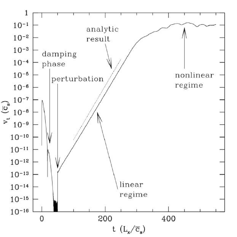
Figure 2: Evolution of $v_{t}$ as a function of time for Run 2 (external potential, non-rotating frame).

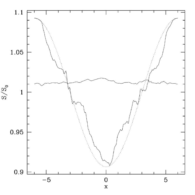
Figure 3: Plot of $N_{x}^{2}$ (left) and $S$ (right) as a function of $x$ for Run 2. Both are averaged over $y$. The dotted line shows the equilibrium profile, and the solid lines show snapshots during the nonlinear regime. Growth initially occurs at the minimum in $N_{x}^{2}$, and the entropy eventually settles to a nearly-constant value.

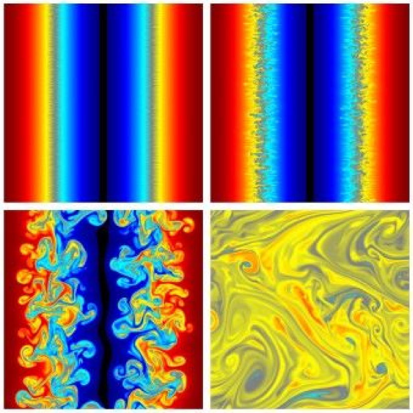
Figure 4: Snapshots of the entropy in the nonlinear regime for Run 2, indicating maximum growth for modes near the grid scale and the eventual turnover of the equilibrium entropy profile to its average value. Dark shades indicate values above (red in electronic edition) and below (blue in electronic edition) the average value.

A plot of $v_{t}$ as a function of time is given in Figure 2, showing the initial damping followed by exponential growth in the linear regime. The analytic growth rate is shown on the plot for comparison. A least-squares fit of the data in the range $100\leq t\Omega\leq 250$ yields a measured growth rate of $0.0978$. Figure 3 shows a cross section of $N_{x}^{2}$ as a function of $x$ after the instability has begun to set in, along with cross sections of the entropy early and late in the nonlinear regime. The growth is initially concentrated near the minimum points in $N_{x}^{2}(x)$. Eventually the entropy turns over completely and settles to a nearly constant value. Figure 4 shows two-dimensional snapshots of the entropy in the nonlinear regime. Runs with the same equilibrium profile except $\gamma-\Gamma\geq 0$ are stable. There is also a long-wavelength axisymmetric instability that is present for $\gamma-\Gamma<0$ even in the absence of the small-scale nonaxisymmetric modes. We measure its growth rate to be $0.07$. Due to the long-wavelength nature of these modes, they are not treatable by a local linear analysis.

5.2 External Potential in Rotating Frame

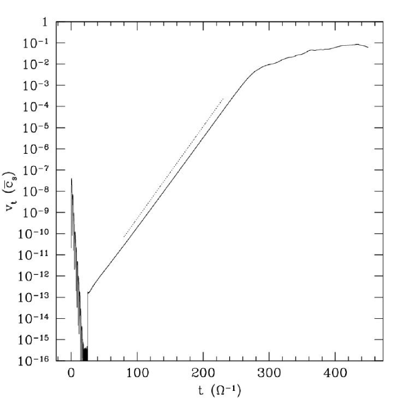
Figure 5: Evolution of $v_{t}$ as a function of time for Run 3 (external potential, rotating frame). The dotted line shows the expected growth rate.

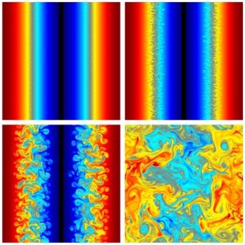
Figure 6: Snapshots of the entropy in the nonlinear regime for Run 3. Dark shades indicate values above (red in electronic edition) and below (blue in electronic edition) the average value.

We have performed the same test as described in §5.1 in a rotating frame ($\Omega=1$ in equation [2]). Figure 5 shows the exponential growth in the linear regime for this run, with a measured growth rate of $0.0977$. Figure 6 shows snapshots of the entropy in the nonlinear regime. The results are similar to the nonrotating case, except that 1) rotation suppresses the long-wavelength axisymmetric instability; 2) the nonlinear outcome exhibits more coherent structures in the rotating case including transient vortices; and 3) these coherent structures eventually become unstable to a Kelvin-Helmholz-type instability.

5.3 Uniform Rotation

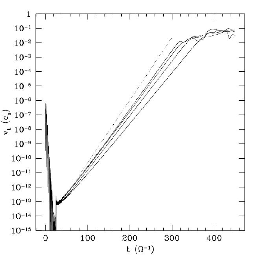
Figure 7: Evolution of $v_{t}$ as a function of time for Run 4 ($q=0$). The dotted line shows the expected growth rate, and the solid lines are runs with (in order of increasing growth) $L_{y}=12$, $6$, $3$ and $1.5$.

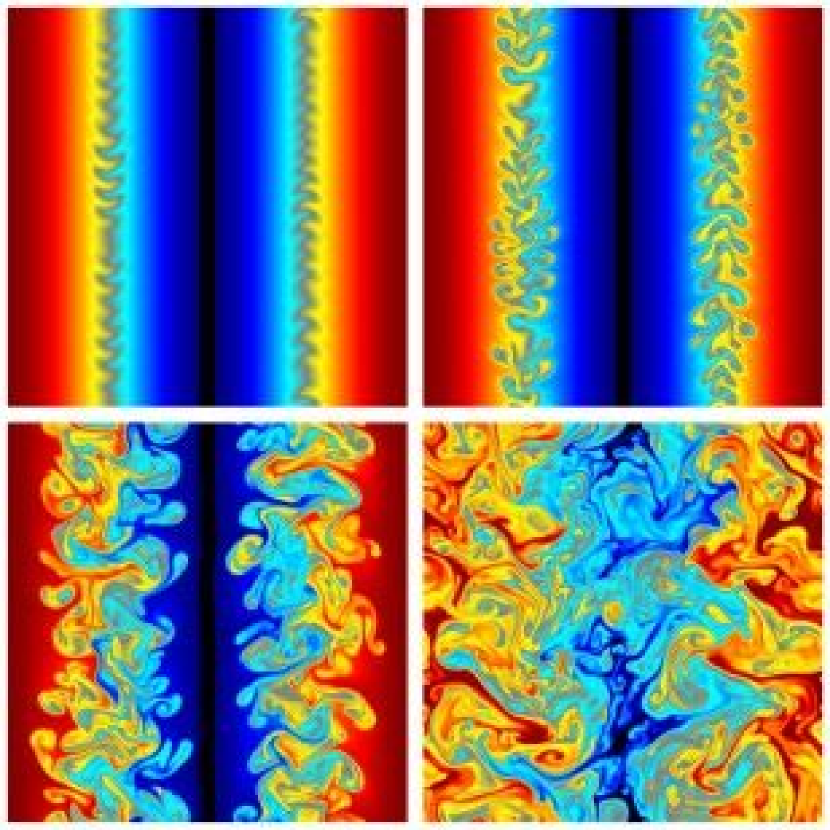
Figure 8: Snapshots of the entropy in the nonlinear regime for Run 4. Dark shades indicate values above (red in electronic edition) and below (blue in electronic edition) the average value. Notice that the maximum growth does not occur for modes at the grid scale.

Having demonstrated the viability of simulating convective instability in the local model, we now turn to the physically-realistic equilibrium described in §4. We begin by setting the shear parameter $q$ to zero in order to make contact with the results of §§5.1 and 5.2. This is analogous to a disk in uniform rotation. The other model parameters are the same as for the previous runs. While there is still an effective shear $-0.05\lesssim{\tilde{q}}\lesssim 0.05$, near ${\tilde{q}}=0$ one expects the modes to obey equation (26) in the WKB limit. Figures 7 and 8 give the linear and nonlinear results for this run. The measured growth rate in the linear regime is $0.0809$.

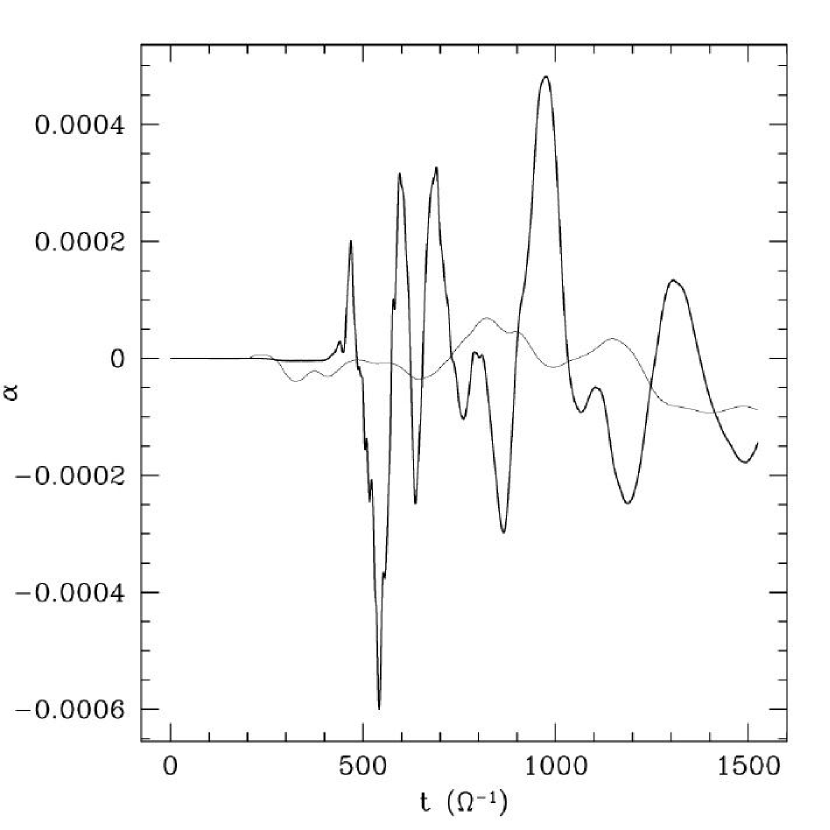
Figure 9: Evolution of the dimensionless angular momentum flux due to radial convection. The thin line is the data boxcar-smoothed over an interval $\Delta t=500\Omega^{-1}$.

Consistent with results from numerical simulations of vertical convection (Stone & Balbus, 1996; Cabot, 1996), the angular momentum transport associated with radial convection is slightly inwards. Figure 9 shows the evolution of the dimensionless angular momentum flux

$$\alpha\equiv{1\over{L_{x}L_{y}{\langle}P_{0}{\rangle}}}\int\Sigma\delta v_{x}\delta v_{y}dxdy,$$ (34)

where ${\langle}P_{0}{\rangle}$ is the radial average of the equilibrium pressure, for an extended version of Run 4. The thin line is a version of the data that has been boxcar-smoothed to show the bias toward a negative flux.

There are two reasons for the larger error in the measured growth rate for this run: 1) the equilibrium velocity gives rise to numerical diffusion due to the motion of the fluid variables with respect to the grid; and 2) since the growing modes are being advected in the azimuthal direction, the maximum growth does not occur at the grid scale. The latter effect can be seen in Figure 8; several grid cells are required for a well-resolved wavelength. In order to resolve smaller wavelengths, we have repeated this run with $L_{y}=6$, $3$ and $1.5$. The results are plotted in Figure 7 along with the results from the $L_{y}=12$ run. The measured growth rate for the $L_{y}=1.5$ run is $0.0924$.

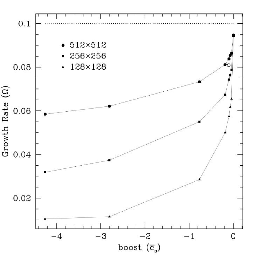
Figure 10: Growth rates as a function of azimuthal boost in a series of runs with an external potential and $N_{x,min}^{2}=-0.01$. The dotted line shows the analytic growth rate from linear theory. The open circle denotes the growth rate that was measured in Run 4, with the boost corresponding to the magnitude of the velocity at the minimum in $N_{x}^{2}$ for Run 3 ($q=0$). The largest boost magnitude corresponds to the velocity at the minimum in $N_{x}^{2}$ for Run 10 ($q=1.5$).

To quantify the effects of numerical diffusion, we have performed a series of tests similar to Run 2 (external potential in a rotating frame) but with an overall boost in the azimuthal direction. Figure 10 shows measured growth rates as a function of boost at three different numerical resolutions. The largest boost magnitude in this plot corresponds to the velocity at the minimum in $N_{x}^{2}$ for a run with $q=1.5$. This highlights the importance of the fluid velocity with respect to the grid in determining numerical damping in ZEUS.

5.4 Shearing Sheet

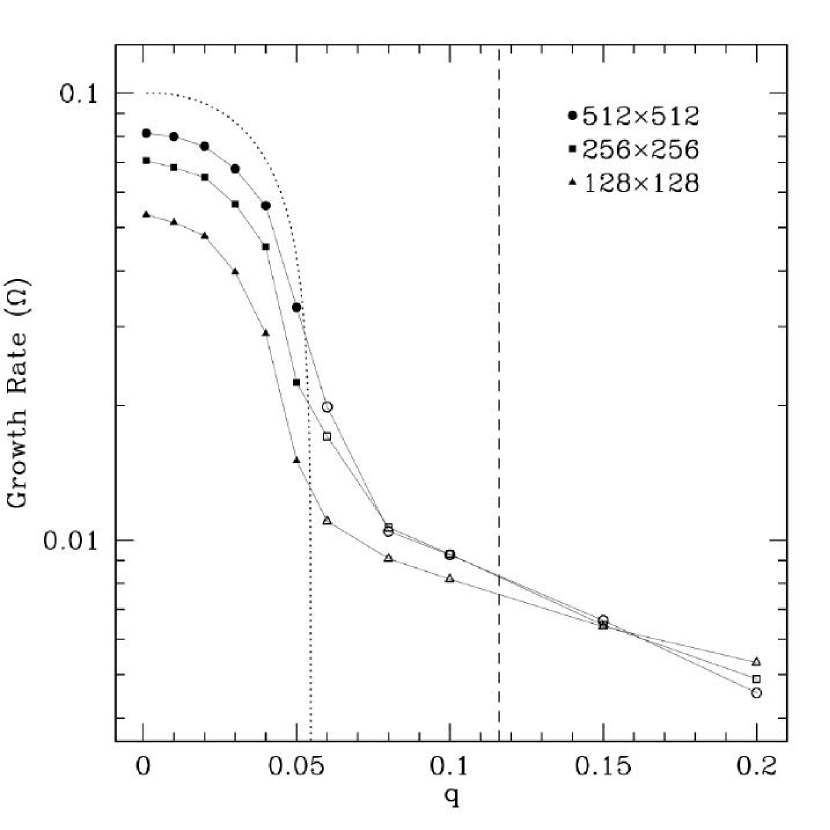
Figure 11: Growth rates as a function of $q$ with $N_{x,min}^{2}=-0.01$. See the text for a discussion.

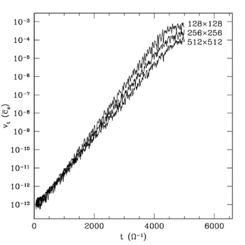
Figure 12: Evolution of $v_{t}$ as a function of time for Run 7 ($q=0.2$ and $N_{x,min}^{2}=-0.01$).

To investigate the effect of differential rotation upon the growth of this instability, we have performed a series of simulations with nonzero $q$. Intuitively, one expects the instability to be suppressed when the shear rate is greater than the growth rate, i.e. for ${\rm Ri}\gtrsim-1$. Figure 11 shows growth rates from a series of runs with $N_{x,min}^{2}=-0.01$ and small, nonzero values of $q$ at three numerical resolutions. This figure clearly demonstrates our main result: convective instability is suppressed by differential rotation. The expected growth rate from linear theory ($\sqrt{|N_{x}^{2}|}$ at ${\tilde{q}}=0$) is shown in Figure 11 as a dotted line. If there is a radial position where ${\tilde{q}}(x)=0$ (i.e., ${\rm Ri}=-\infty$), $v_{t}$ at that position looks similar to that of the previous runs (very little deviation from a straight line); these measurements are indicated on the plot with solid points. For $q\gtrsim 0.055$ there is no longer any point where ${\tilde{q}}(x)=0$; in that case $v_{t}$ was measured at the radial average between the minimum in $N_{x}^{2}(x)$ and the minimum in ${\tilde{q}}(x)$, since this is where the maximum growth occured. The data for these measurements, which are indicated in Figure 11 with open points, is not as clean as it is for the runs with ${\rm Ri}=-\infty$ (see Figure 12). All of the growth rate measurements in Figure 11 were obtained by a least-squares fit of the data in the range $1\times 10^{-9}<v_{t}/\bar{c}_{s}<1\times 10^{-5}$. The dashed line in Figure 11 indicates the value of $q$ for which ${\rm Ri}_{min}=-1$.

Some of the growth in Figure 11 appears to be due to aliasing. This is a numerical effect in finite-difference codes that results in an artificial transfer of power from trailing shwaves into leading shwaves as the shwave is lost at the grid scale. One expects aliasing to occur approximately at intervals of

$$\Delta\tilde{\tau}=\frac{N_{x}}{n_{y}}\frac{L_{y}}{L_{x}},$$ (35)

where $n_{y}$ is the azimuthal shwave number. This interval corresponds to $\Delta\tilde{k}_{x}(t)=2\pi/dx$, where $dx=L_{x}/N_{x}$ is the radial grid scale. Based upon expression (35), aliasing effects should be more pronounced at lower numerical resolution because the code has less time to evolve a shwave before the wavelength of the shwave becomes smaller than the grid scale. It can be seen from the far-right data point in Figure 11 (Run 7 in Table 1) that the measured growth rate decreases with increasing resolution. The evolution of $v_{t}$ for this run is shown in Figure 12.

The effects of aliasing can be seen explicitly by evolving a single shwave, as was done for our linear theory test (Figure 1). Figure 13 shows the evolution of the density perturbation for a single shwave using the same parameters that were used for Run 7: $L_{x}=L_{y}=12$, $N_{x,min}^{2}=-0.01$ and $q=0.2$. The initial shwave vector used was $(k_{x0},k_{y})=(-8\pi/L_{x},8\pi/L_{y})$. This corresponds to $n_{y}=4$, and the expected aliasing interval (35) is therefore $\Delta\tilde{\tau}=N_{x}/4$. Runs at three numerical resolutions are plotted in Figure 13, and the aliasing interval at each resolution is consistent with expression (35). It is clear from Figure 13 that a lower resolution results in a larger overall growth at the end of the run. It also appears that the growth seen in Figure 13 requires a negative entropy gradient. We have performed this same test with $N_{x}^{2}>0$, and while aliasing occurs at the same interval, there is no overall growth in the perturbations. This may be due to the fact that the perturbations decay asymptotically for $N_{x}^{2}>0$ (see expression [30]).

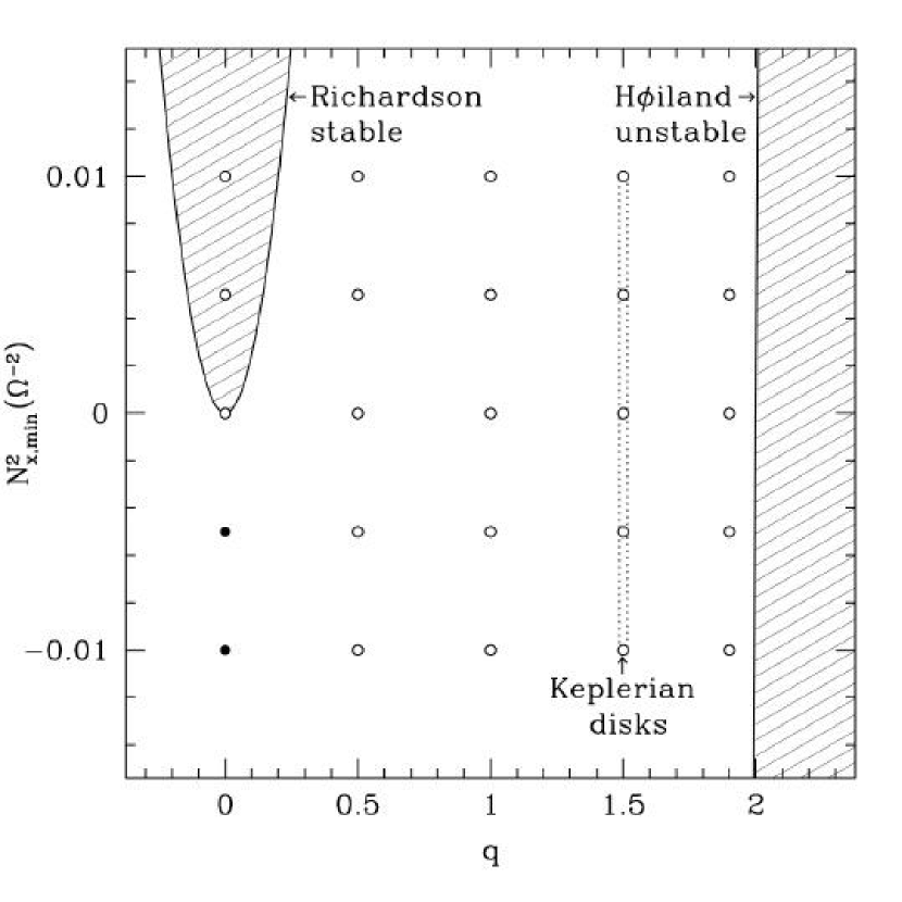
Figure 14: Parameter space surveyed in a search for nonlinear instabilities. Closed (open) circles denote runs that were unstable (stable). The only instability found was convective instability for ${\tilde{q}}\simeq 0$ and $N_{x}^{2}<0$ (${\rm Ri}\rightarrow-\infty$). (We do not include on this plot the runs shown in Figure 11.)

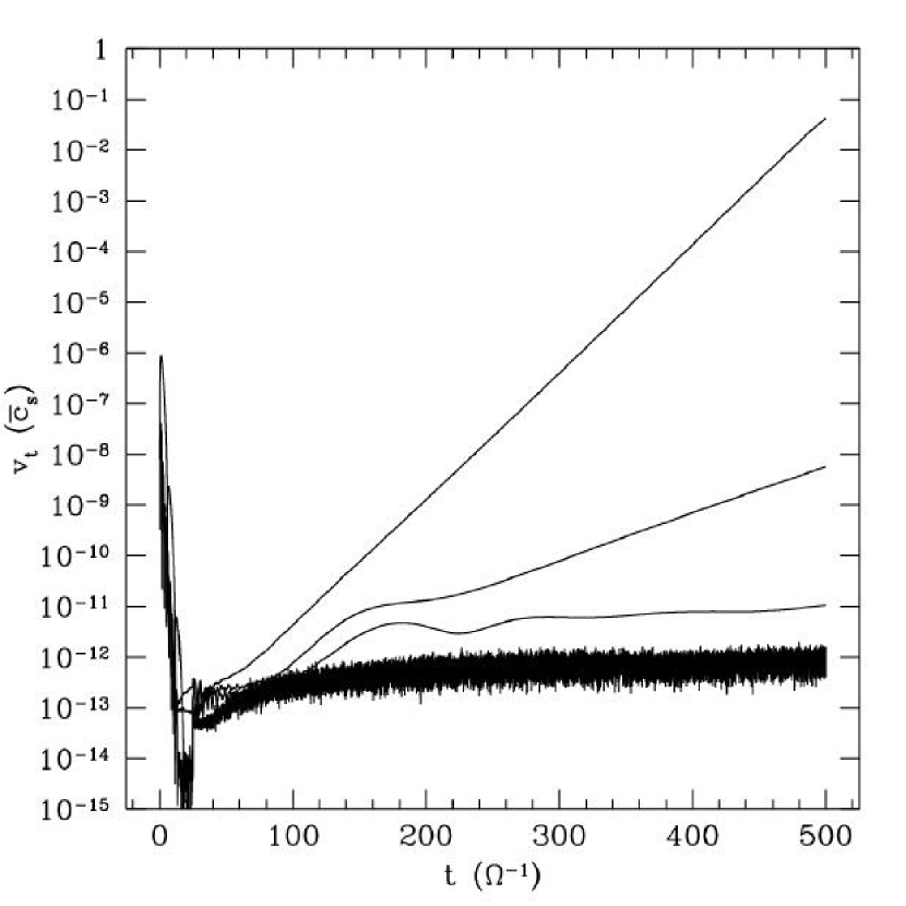
Figure 15: Evolution of $v_{t}$ as a function of time for Run 10 ($q=1.5$, $N_{x,min}^{2}=-0.01$). Also shown are runs with $q=0$ and an overall boost equivalent to the velocity at the minimum in $N_{x}^{2}$ for Run 10, for $N_{x,min}^{2}=-0.01$ (measured growth rate of $0.058$), $N_{x,min}^{2}=-0.003$ (measured growth rate of $0.021$) and $N_{x,min}^{2}=-0.001$ (measured growth rate of $0.0025$).

Figure 14 summarizes the parameter space we have surveyed, indicating that there is instability only for ${\tilde{q}}\simeq 0$ and $N_{x}^{2}<0$. The numerical resolution in all of these runs is $512\times 512$. Figure 15 shows the evolution of the radial velocity in Run 10, a run with realistic parameters for a disk with a nearly-Keplerian rotation profile and radial gradients on the order of the disk radius: $q=1.5$ and $N_{x,min}^{2}=-0.01$ (corresponding to ${\rm Ri}\simeq-0.004$). Clearly no instability is occurring on a dynamical timescale. This plot is typical of all runs for which the evolution was stable. To give a sense for the minimum growth rate that we are able to measure, we have also plotted in Figure 15 the results from several unstable runs with $q=0$ and a boost equivalent to the velocity at the minimum in $N_{x}^{2}$ for Run 10. It is difficult to measure a growth rate for the smallest value of $N_{x,min}^{2}$, but it is clear that there is activity present in this run which does not occur in the stable run. Based upon Figure 15, a conservative estimate for the minimum growth rate that should be detectable in our simulations is $0.0025\Omega$.

6 Implications

Our results are consistent with the idea that nearly-Keplerian disks are stable, or at most very weakly unstable, to local nonaxisymmetric disturbances. Because our numerical resolution is finite, we cannot exclude the possibility of instability appearing at even higher resolution. But Figure 11 demonstrates that convective instabilities that are present when the shear is nearly zero are stabilized by differential rotation. Perturbations simply do not have time to grow before they are pulled apart by the shear.

An important implication of our results is that the instability claimed by Klahr & Bodenheimer (2003) is not a linear or nonlinear local nonaxisymmetric instability. Figure 13 suggests that the results of Klahr & Bodenheimer (2003) may be due, at least in part, to aliasing. They use a finite difference code at fairly low numerical resolution ($\leq 128^{2}$), and growth is only observed in runs with a negative entropy gradient. Curvature effects and the effects of boundary conditions, which may also play a role in their global results, cannot be tested in our local model.

In addition to being local, the simulations we have performed are two-dimensional. Interesting vertical structure is likely to develop in three-dimensional simulations, and this may affect our results. At the same time, strong vertical stratification away from the midplane of the disk may enforce two-dimensional behaviour.

Vanneste et al. (1998) calculated three-shwave interactions in the unstratified (incompressible) shearing sheet and found that there is feedback from trailing shwaves into leading shwaves for a small subset of initial shwave vectors. It would be of interest to revisit this calculation in the stratified shearing sheet. One key difference between the stratified and unstratified shearing-sheet models is that in the latter case all linear perturbations decay after their transient growth, whereas in the former case the density perturbation does not decay. Even though the feedback in Figure 13 is due to a numerical effect, these results show that feedback in the stratified shearing sheet can result in overall growth.

This work was supported by NSF grant AST 00-03091, PHY 02-05155, NASA grant NAG 5-9180, and a Drickamer Fellowship for BMJ.

Table 1: Summary of Code Runs

Run	Description	$L_{y}$ ($L_{x}=12$)	$N_{y}$	$N_{x}$	Figure(s)
1	Linear theory test	$0.375$	$16,32,64$	$64N_{y}$	1
2	External potential, $\Omega=0$	$12$	$512$	$N_{y}$	2-4
3	External potential, $\Omega=1$	$12$	$512$	$N_{y}$	5-6
4	Uniform rotation ($q=0$)	$12,6,3,1.5$	$512$	$N_{y}$	7-9
5	External potential, $\Omega=1$, boost	$12$	$128,256,512$	$N_{y}$	10
6	Small shear ($-\infty\lesssim{\rm Ri}\lesssim-1$)	$12$	$128,256,512$	$N_{y}$	11
7	Small shear ($q=0.2,{\rm Ri}\gtrsim-1$)	$12$	$128,256,512$	$N_{y}$	12
8	Aliasing ($q=0.2,{\rm Ri}\gtrsim-1$)	$12$	$128,256,512$	$N_{y}$	13
9	Parameter survey	$12$	$512$	$N_{y}$	14
10	Keplerian disk ($q=1.5,{\rm Ri}\simeq-0.004$)	$12$	$512$	$N_{y}$	15

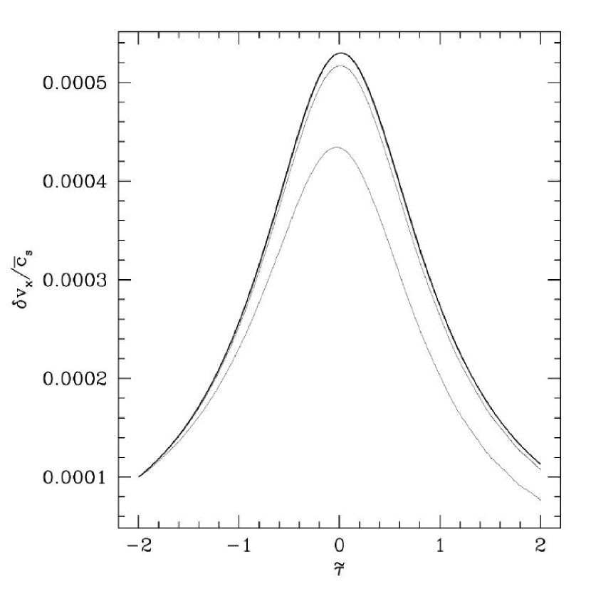
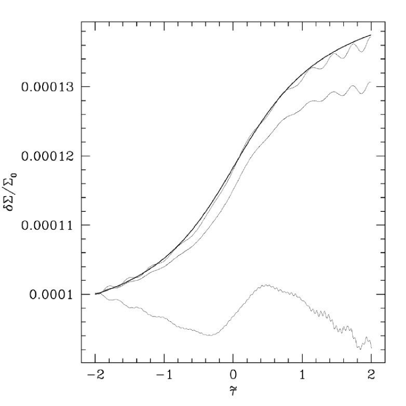
Figure 1: Evolution of a vortical shwave amplitude in the radially-stratified shearing sheet (Run 1). The left panel shows the radial velocity perturbation and the right panel shows the density perturbation. The heavy line in each panel is the analytic result, and the light lines are runs with a numerical resolution of (in order of increasing accuracy) $N_{x}\times N_{y}=1024\times 16$, $2048\times 32$ and $4096\times 64$. The number of grid cells are chosen so that the shwave initially has the same number of grid cells per wavelength in both the $x$ and $y$ directions. The results are shown for a test point at the minimum in $N_{x}^{2}$.

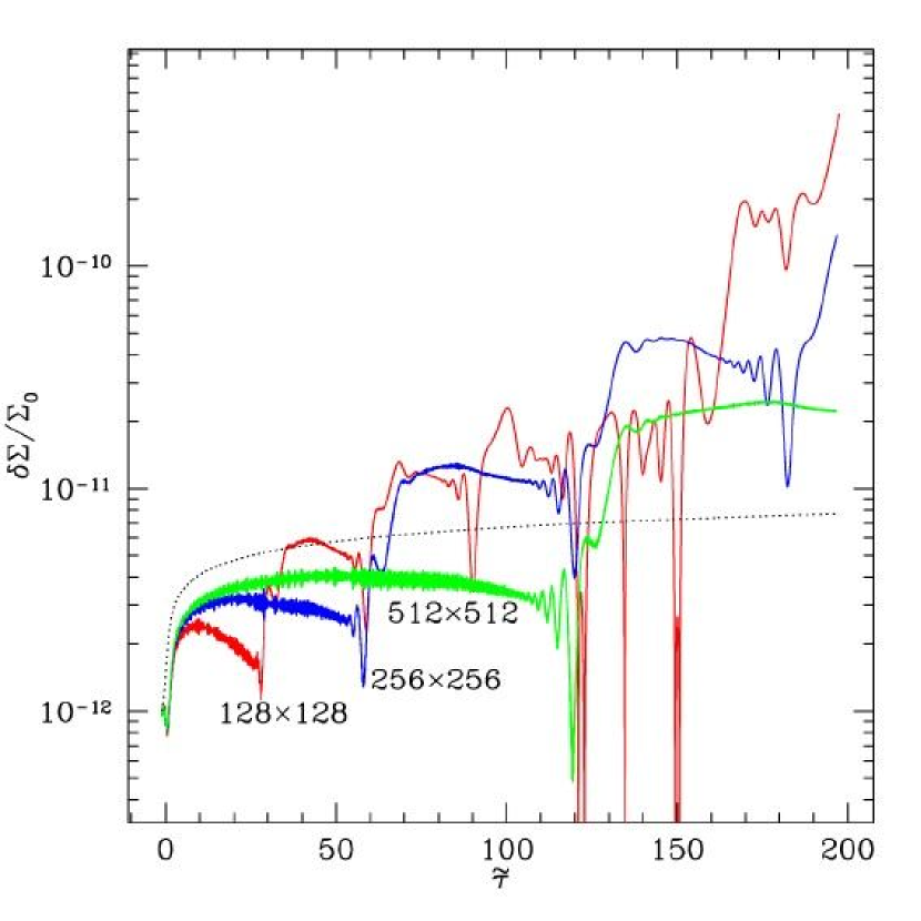
Figure 13: Evolution of the density perturbation for a single shwave with $q=0.2$, $N_{x,min}^{2}=-0.01$ and $L_{y}=L_{x}$ (Run 8). The linear theory result is shown as a dotted line, along with results at three numerical resolutions: $128^{2}$, $256^{2}$ and $512^{2}$ (red, blue and green, respectively, in electronic edition). Aliasing occurs when $\tilde{k}_{x}(t)=2\pi/dx$. The overall growth, which is greater at lower numerical resolution, requires $N_{x}^{2}<0$.

References

- Afshordi, Mukhopadhyay, & Narayan (2004) Afshordi, N., Mukhopadhyay, B., & Narayan, R. 2004, ArXiv Astrophysics e-prints, astro-ph/0412194
- Balbus & Hawley (1998) Balbus, S. A. & Hawley, J. F. 1998, Reviews of Modern Physics, 70, 1
- Balbus & Terquem (2001) Balbus, S. A., & Terquem, C. 2001, ApJ, 552, 235
- Binney & Tremaine (1987) Binney, J., & Tremaine, S. 1987, Princeton, NJ, Princeton University Press, 1987, 747pp
- Blaes & Balbus (1994) Blaes, O. M., & Balbus, S. A. 1994, ApJ, 421, 163
- Cabot (1996) Cabot, W. 1996, ApJ, 465, 874
- Chagelishvili, Zahn, Tevzadze, & Lominadze (2003) Chagelishvili, G. D., Zahn, J.-P., Tevzadze, A. G., & Lominadze, J. G. 2003, A&A, 402, 401
- Chimonas (1970) Chimonas, G. 1970, J. Fluid Mech., 43, 833
- Desch (2004) Desch, S. J. 2004, ApJ, 608, 509
- Fleming et al. (2000) Fleming, T. P., Stone, J. M., & Hawley, J. F. 2000, ApJ, 530, 464
- Fleming & Stone (2003) Fleming, T., & Stone, J. M. 2003, ApJ, 585, 908
- Gammie (1996) Gammie, C.F. 1996, ApJ, 457, 355
- Gammie (2001) Gammie, C.F. 2001, ApJ, 553, 174
- Gammie & Menou (1998) Gammie, C. F. & Menou, K. 1998, ApJ, 492, L75
- Goldreich, Goodman, & Narayan (1986) Goldreich, P., Goodman, J., & Narayan, R. 1986, MNRAS, 221, 339
- Goldreich & Lynden-Bell (1965) Goldreich, P. & Lynden-Bell, D. 1965, MNRAS, 130, 125
- Goldreich & Tremaine (1978) Goldreich, P. & Tremaine, S. 1978, ApJ, 222, 850
- Hawley, Gammie, & Balbus (1995) Hawley, J. F., Gammie, C. F., & Balbus, S. A. 1995, ApJ, 440, 742
- Howard (1961) Howard, L. N. 1961, Journal of Fluid Mechanics, 10, 509
- Jin (1996) Jin, L. 1996, ApJ, 457, 798
- Johnson & Gammie (2005) Johnson, B. M. & Gammie, C. F. 2005, ApJ, submitted
- Julian & Toomre (1966) Julian, W. H. & Toomre, A. 1966, ApJ, 146, 810
- Klahr & Bodenheimer (2003) Klahr, H. H. & Bodenheimer, P. 2003, ApJ, 582, 869
- Klahr (2004) Klahr, H. 2004, ApJ, 606, 1070
- Kunz & Balbus (2004) Kunz, M. W. & Balbus, S. A. 2004, MNRAS, 348, 355
- Masset (2000) Masset, F. 2000, A&AS, 141, 165
- Menou (2000) Menou, K. 2000, Science, 288, 2022
- Miles (1961) Miles, J. W. 1961, Journal of Fluid Mechanics, 10, 496
- Papaloizou & Pringle (1984) Papaloizou, J. C. B. & Pringle, J. E. 1984, MNRAS, 208, 721
- Salmeron & Wardle (2003) Salmeron, R., & Wardle, M. 2003, MNRAS, 345, 992
- Salmeron (2004) Salmeron, R., Ph.D. Thesis, University of Sydney.
- Sano & Stone (2002a) Sano, T., & Stone, J. M. 2002, ApJ, 570, 314
- Sano & Stone (2002b) Sano, T., & Stone, J. M. 2002, ApJ, 577, 534
- Stone & Balbus (1996) Stone, J. M., & Balbus, S. A. 1996, ApJ, 464, 364
- Stone, Gammie, Balbus, & Hawley (2000) Stone, J. M., Gammie, C. F., Balbus, S. A., & Hawley, J. F. 2000, Protostars and Planets IV, 589
- Stone & Norman (1992) Stone, J. M. & Norman, M. L. 1992, ApJS, 80, 753
- Umurhan & Regev (2004) Umurhan, O. M. & Regev, O. 2004, A&A, 427, 855
- Vanneste et al. (1998) Vanneste, J., Morrison, P. J., & Warn, T. 1998, Physics of Fluids, 10, 1398
- Wardle (1999) Wardle, M. 1999, MNRAS, 307, 849