Plasma Diagnostics of Active Region Evolution and Implications for Coronal Heating

Abstract

A detailed study is presented of the decaying solar active region NOAA 10103 observed with the Coronal Diagnostic Spectrometer (CDS), the Michelson Doppler Imager (MDI) and the Extreme-ultraviolet Imaging Telescope (EIT) onboard the Solar and Heliospheric Observatory (SOHO). Electron density maps formed using Si x(356.03 Å/347.41 Å) show that the density varies from $\sim$10¹⁰ cm^-3 in the active region core, to $\sim$7$\times$10⁸ cm^-3 at the region boundaries. Over the five days of observations, the average electron density fell by $\sim$30 per cent. Temperature maps formed using Fe xvi(335.41 Å)/Fe xiv(334.18 Å) show electron temperatures of $\sim$2.34$\times$10⁶ K in the active region core, and $\sim$2.10$\times$10⁶ K at the region boundaries. Similarly to the electron density, there was a small decrease in the average electron temperature over the five day period. The radiative, conductive, and mass flow losses were calculated and used to determine the resultant heating rate ($P_{H}$). Radiative losses were found to dominate the active region cooling process. As the region decayed, the heating rate decreased by almost a factor of five between the first and last day of observations. The heating rate was then compared to the total unsigned magnetic flux ($\Phi_{tot}=\int dA|B_{z}|$), yielding a power-law of the form $P_{H}\sim\Phi_{tot}^{0.81\pm 0.32}$. This result suggests that waves rather than nanoflares may be the dominant heating mechanism in this active region.

1 INTRODUCTION

Since the discovery of highly ionized species of iron in the solar corona in the 1930’s, physicists have been puzzled by the high temperatures observed in the outer solar atmosphere (Edlen, 1937). It is widely accepted that the magnetic field plays a fundamental role in the heating process, but precise measurements of the coronal magnetic field are currently impossible. Indirect methods are therefore adopted which rely on measurable quantities such as the electron temperature, density and photospheric magnetic flux. These measurements can then be compared to theoretical predictions.

Models for coronal heating typically belong to one of two broad categories. In wave (AC) heating, the large-scale magnetic field essentially acts as a conduit for small-scale, high-frequency Alfvèn waves propagating into the corona. For constant Alfvèn wave amplitude $\langle v^{2}\rangle$, the total power dissipated in an active region is,

$$P_{H}=\sqrt{\frac{\rho}{4\pi}}\langle v^{2}\rangle\Phi_{tot}~{}~{}{\rm~{}ergs~{}s^{-1}},$$ (1)

where $\rho$ is the mass density, and $\Phi_{tot}$ is the total unsigned magnetic flux,

$$\Phi_{tot}=\int dA|B_{z}|~{}~{}{\rm~{}Mx},$$ (2)

where $B_{z}$ is the longitudinal component of the magnetic field.

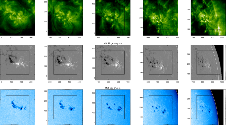
Figure 1: The evolution of NOAA 10103 during September 10–14. Top row: EIT (195 Å) images. Middle row: MDI magnetograms. Bottom row: MDI continuum images. The inner boxes in each image denote the field-of-view of the CDS raster.

In stress (DC) heating, the coronal magnetic field stores energy in the form of electric currents until it can be dissipated, e.g., by nanoflares (Parker, 1988). The total power can be estimated by,

$$P_{H}\sim|v|\Phi_{tot}^{2}~{}~{}{\rm~{}ergs~{}s^{-1}},$$ (3)

and the constant of proportionality describes the efficiency of magnetic dissipation, which might involve the random footpoint velocity, $v$ (Parker, 1983), or simply the geometry (Browning, Sakuria, & Priest, 1986; Fisher et al., 1998).

Several authors have linked the photospheric magnetic flux to EUV and X-ray line intensity. Gurman et al. (1974) found that the line intensity of Mg x (624.94 Å) was proportional to the magnetic flux density. Schrijver (1987) related the integrated intensities of chromospheric, transition region, and coronal lines to the total magnetic flux by a power law, the index of which was dependent on the scale height. This result was later confirmed by Fisher et al. (1998), who showed that X-ray luminosity is highly correlated with the total unsigned magnetic flux. Van Driel-Gesztelyi et al. (2003) also showed a power-law relationship between the mean X-ray flux, temperature, and emission measure, and the mean magnetic field by studying the long-term evolution of an active region over several rotations, at times when there were no significant brightenings.

In this paper, we study the evolution of a decaying active region using the diagnostic capabilities of the Coronal Diagnostic Spectrometer (CDS; Harrison et al. 1995) and Michelson Doppler Imager (MDI; Scherrer et al. 1995) onboard SOHO. Using the temperatures, densities, and dimensions of the active region, the heating rate is calculated and compared to the total unsigned magnetic flux. These results can be put in the context of theoretical models. Section 2 gives a brief overview of the active region, a summary of the instruments involved, and a description of the data analysis techniques. Our results are given in Section 3, and discussion and conclusions in Section 4.

2 OBSERVATIONS AND DATA ANALYSIS

NOAA 10103 was observed by CDS, EIT, and MDI for five consecutive days during 2002 September 10–14. Fig. 1 shows the general evolution of the region over that period.

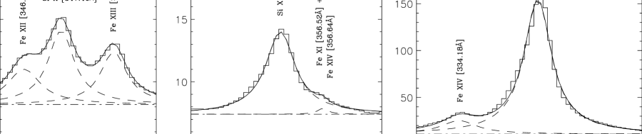
Figure 2: Portions of the CDS spectra from NOAA 10103 on September 10, together with backgrounds (horizontal dot-dash lines) and broadened Gaussian fits.

2.1 The Coronal Diagnostic Spectrometer

EUV spectra were obtained with the CDS instrument, which is a dual spectrometer that can be used to obtain images with a spatial resolution of $\sim$8 arcsec. The Normal Incidence Spectrometer (NIS), used in this study, is a stigmatic spectrometer which forms images by moving the solar image across the slit using a scan mirror. The spectral ranges of NIS (308–381 Å and 513–633 Å) include emission lines formed over a wide range of temperatures, from $\sim$10⁴ K at the upper chromosphere, through the transition region, to $\sim$10⁶ K at the corona. The details of the az_ddep1 observing sequence used in this study can be found in Table 1.

Table 1: Details of the CDS az_ddep1 observing sequence

Parameter	Value
Date	2002 September 10–14
Region name	NOAA 10103
Instrument	CDS/NIS1
Wavelength range (Å)	332–368
Slit size (arcsec2)	4.064$\times$240
Area imaged (arcsec2)	243.84$\times$240
Exposure time (s)	50
Number of slit positions	60

The raw CDS data were cleaned to remove cosmic rays, and calibrated to remove the CCD readout bias and convert the data into physical units of photons cm^-2 s^-1 arcsec^-2. Due to the broadened nature of post-recovery CDS spectra, the emission lines were fitted with modified Gaussian profiles as described by Thompson (1999). The Gaussian term was defined as,

$$G(\lambda)=exp\left[-\frac{1}{2}\left(\frac{\lambda-\lambda_{0}}{\sigma}\right)^{2}\right],$$ (4)

and the wings by,

$$W(\lambda)=\frac{1}{\left(\frac{\lambda-\lambda_{0}}{\sigma^{\prime}}\right)^{2}+1},$$ (5)

where $\lambda$ is the wavelength, $\lambda_{0}$ is the central wavelength of the line, $\sigma$ is the Gaussian width, and $\sigma^{\prime}$ is the FWHM.

The combined function describing the line profile can be expressed as,

$$B(\lambda)=I[(1-a)G(\lambda)+aW(\lambda)],$$ (6)

where $I$ is the amplitude of the line profile and $a$ can be the amplitude of the red or the blue wing. The line flux is then given by,

$$\int B(\lambda)d\lambda = I\sigma\left[\left(1-\frac{a_{red}}{2}\left(1+\frac{a_{blue}}{a_{red}}\right)\right)\sqrt{2\pi}\right.$$ (7)

$$+ \left.a_{red}\left(1+\frac{a_{blue}}{a_{red}}\right)\pi\sqrt{2\ln(2)}\right].$$

These broadened Gaussian profiles were then fitted to emission lines in three wavelength intervals using the xcfit routine in the CDS branch of the SolarSoftWare tree (SSW; Freeland & Handy 1998; see Fig. 2). Two of the intervals were centreed on each of the density sensitive Si x (347.41 Å) and Si x (356.03 Å) lines, while the third contained the temperature sensitive Fe xiv (334.18 Å) and Fe xvi (335.41 Å) pair. Due to the relatively low intensity of Fe xiv (334.18 Å) compared to that of the adjacent Fe xvi (335.41 Å) transition, an upper constraint on the width of $\sigma$ = 0.4 Å (FWHM = 0.17 Å) was placed on the Fe xiv line. The primary lines, their formation temperatures, transitions, and rest wavelengths are given in Table 2.

Table 2: Ions, Formation Temperatures, Transitions and Wavelengths of Emission Lines Identified in This Work

Ion	Log Te	Transition	$\lambda$/Å
Si x	6.1	2s22p2 3P1/2–2s2p2 2D3/2	347.41
Si x	6.1	2s22p 3P3/2–2s2p2 2D3/2,5/2	356.03
Fe xiv	6.3	3s23p 2P1/2–3s3p2 2D3/2	334.18
Fe xvi	6.4	3s 2S1/2–3p 2P3/2	335.41
Fe xvii	6.7	2p5 3s 3P1–2p5 3p 1D2	347.85

2.2 The Michelson Doppler Interferometer

Magnetic field measurements were taken by the MDI instrument, which images the Sun on a 1024 $\times$ 1024 pixel CCD camera through a series of increasingly narrow filters. The final elements, a pair of tunable Michelson interferometers, enable MDI to record filtergrams with a FWHM bandwidth of 94 mÅ. Several times each day, polarizers are inserted to measure the line-of-sight magnetic field. In this paper, 5-minute-averaged magnetograms of the full disk were used, with a 96 minute cadence and a pixel size of 2 arcsec.

Berger & Lites (2003) analyzed Advanced Stokes Polarimeter (ASP) and MDI magnetograms, and found that MDI underestimates the magnetic flux densities by a factor of 1.45 for values below 1200 G. For flux densities higher than 1200 G, this underestimation becomes nonlinear, with the MDI fluxes saturating at $\sim$1300 G. Values below 1200 G were therefore corrected by multiplying by 1.45, and values above 1200 G were approximately corrected by multiplying by a factor of 1.9 (Green et al., 2003).

Before calculating the total unsigned magnetic flux, two final corrections were applied to the data. The first results from the fact that the measured line-of-sight flux deviates more and more from a radial measurement as one approaches the limb. For simplicity, we assume that magnetic fields in the photosphere are predominantly radial. Then, the radial field strength becomes equal to the line-of-sight field strength times $1/\cos{\theta}$, where $\theta$ is the heliocentric distance of the region from Sun centre.

Active region areas, $A$, were calculated by counting all pixels above 500 G and multiplying by the appropriate factor to obtain the active region area in cm². This threshold value for the magnetic field was found to adequately separate active region structures from neighbouring areas of quiet-Sun and plage. As the region approached the limb, the effects of foreshortening became significant. Measured areas were therefore corrected by dividing by $\cos{\theta}$. The resulting total unsigned flux was then calculated using Equation (2).

Modern high resolution space based instruments, such as the Transition Region and Coronal Explorer (TRACE), have been used by Aschwanden et al. (2001) to show that coronal loops observed in different bandpasses are not necessarily cospatial. Due to the coarse resolution of CDS, we make the assumption that active regions occupy a hemispherical volume, $V=2/3~{}\pi^{-1/2}A^{3/2}$, with a mean loop length of $L=\sqrt{\pi A}$.

Figure 3: The cosine-corrected active region area, total magnetic flux density, and total magnetic flux for September 10–14.

3 RESULTS

3.1 Morphology and Magnetic Field

The top row of Fig. 1 shows a series of 360 $\times$360 arcsec EIT images obtained in the 195 Å bandpass. The first three images show a number of loops to the south and north of the region, which are not visible from 2002 September 13 onwards. On September 10, the MDI magnetogram shows a simple bipolar $\beta$ region, which is then classified as a $\beta\gamma$ on the following day. The region subsequently decreased in both size and complexity as it approached the west limb. The overall decay of the active region is clearest in the MDI continuum images in the bottom row of Fig. 1.

Table 3 and Fig. 3 show the decay of the region in terms of the cosine-corrected area and magnetic flux for September 10–14. The region was observed to have an initial area of 1.26$\times$10¹⁹ cm², which fell to 6.54$\times$10¹⁸ cm² by September 14. The total unsigned magnetic flux density also shows a similar trend, falling from close to 4.80$\times$10⁵ Mx cm² to 1.40$\times$10⁵ Mx cm². The product of the region area times the total magnetic flux density is then given in the bottom panel of Fig. 3. As the region decays, the total unsigned magnetic flux falls off by a factor of 5–6 over the five days from September 10 to 14.

3.2 Electron Densities

Electron density maps were generated using the Si x (356.03 Å/347.41 Å) ratio in conjunction with theoretical data from the chianti v4.2 atomic database (Dere et al., 1997). Fig. 4 shows a plot of the density sensitive Si x (356.03 Å/347.40 Å) ratio together with the expected range of densities in an active region of this size and class.

The density maps, presented in the second row of Fig. 5, show values of $\sim$10¹⁰ cm^-3 in the active region core, and $\sim$7$\times$10⁸ cm^-3 in the region boundaries. These are in good agreement with previous active region density measurements (Gallagher et al. 2001; Warren & Winebarger 2003). Densities in the core were observed to fall from $\sim$10¹⁰ on September 10 to 3.9$\times$10⁹ cm^-3 on September 14, excluding the high density limit ($\sim$2.5$\times$10¹⁰ cm^-3) that was reached during a C-class flare on September 13. This behaviour is more evident in the top panel of Fig. 6, which clearly shows that the average electron density changed by $\sim$30 per cent over the five days. Subsequently, plasma that was found to reach the high density limit was excluded from any further calculations. The average electron densities are listed in Table 3.

Figure 4: Theoretical line ratio as a function of density from chianti for Si x (356.03 Å/347.41 Å). The vertical dotted lines denote the typical range of densities expected to be found in an active region.

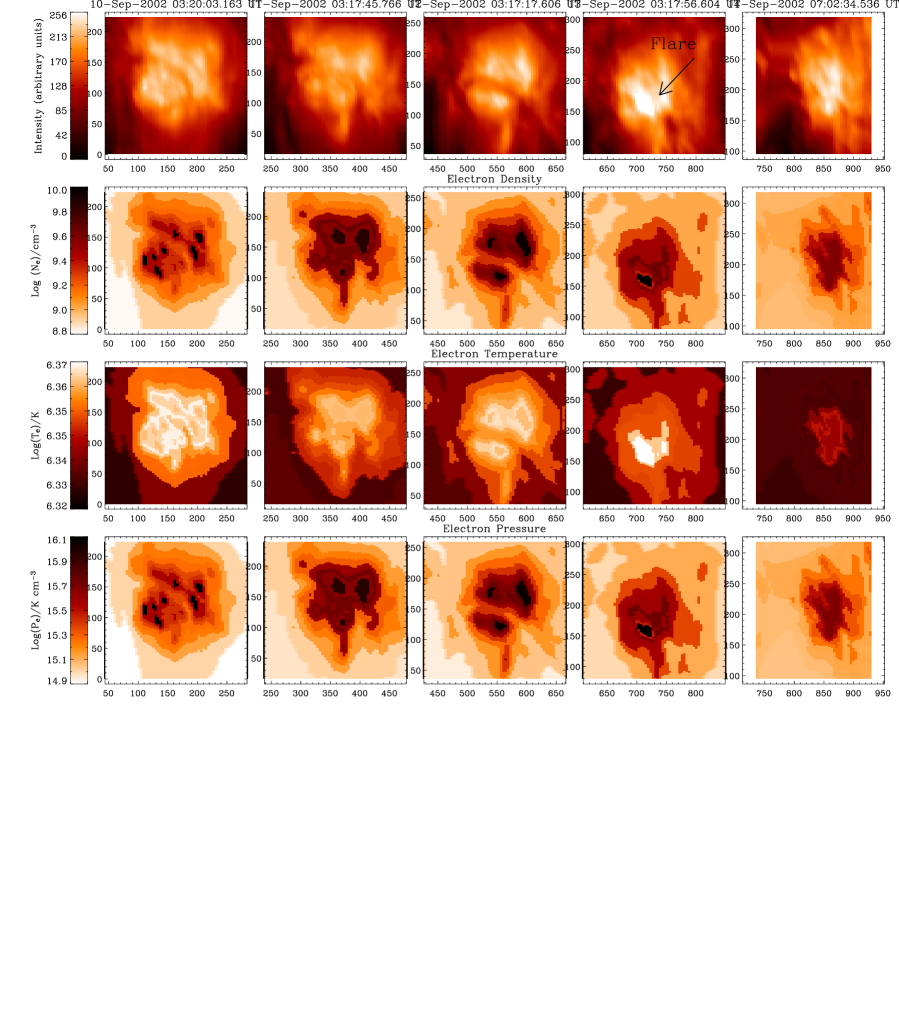
Figure 5: Top row: CDS images of NOAA 10103 over the five days of observations. Second row: Electron density maps derived from the Si x (356.03 Å/347.41 Å) ratio. Third row: Electron temperature maps found from the Fe xvi (335.41 Å)/Fe xiv (334.19 Å) ratio. Bottom row: Electron pressure maps from the product of the density maps with the formation temperature of the Si x lines. The panels for September 13 show the compact brightening.

Table 3: Principal Parameters Derived for NOAA 10103 for 2002 September 10–14

	$\langle N_{e}\rangle$	$\langle T_{e}\rangle$	$\langle P_{e}\rangle$	$A$	$V$	$L$
Date	109cm-3	106K	1015K cm-3	1018cm2	1028cm3	109cm
2002 September 10	2.46$\pm$0.31	2.26$\pm$0.03	3.10$\pm$0.60	12.66$\pm$0.75	1.69$\pm$0.15	6.31$\pm$0.37
2002 September 11	2.71$\pm$0.53	2.24$\pm$0.03	3.41$\pm$0.84	10.23$\pm$0.64	1.23$\pm$0.11	5.66$\pm$0.35
2002 September 12	3.04$\pm$0.79	2.26$\pm$0.03	3.83$\pm$1.16	10.58$\pm$0.76	1.29$\pm$0.14	5.76$\pm$0.41
2002 September 13	2.46$\pm$0.52	2.24$\pm$0.02	3.10$\pm$0.65	9.89$\pm$1.03	1.17$\pm$0.18	5.57$\pm$0.58
2002 September 14	1.87$\pm$0.20	2.16$\pm$0.02	2.35$\pm$0.43	6.54$\pm$1.22	0.62$\pm$0.17	4.53$\pm$0.84
	$P_{R}$	$P_{C}$	$P_{F}$	$P_{H}$	$\Phi_{tot}$
Date	1025ergs s-1	1025erg s-1	1025erg s-1	1025ergs s-1	1024Mx
2002 September 10	3.37$\pm$0.90	0.28$\pm$0.07	0.25$\pm$0.04	3.90$\pm$1.57	5.97$\pm$0.35
2002 September 11	2.97$\pm$1.12	0.19$\pm$0.05	0.37$\pm$0.08	3.53$\pm$1.92	4.01$\pm$0.25
2002 September 12	3.92$\pm$2.07	0.21$\pm$0.06	0.43$\pm$0.12	4.56$\pm$3.10	3.97$\pm$0.28
2002 September 13	2.33$\pm$1.05	0.30$\pm$0.07	0.42$\pm$0.14	2.59$\pm$1.40	2.78$\pm$0.29
2002 September 14	0.71$\pm$0.24	0.07$\pm$0.03	0.18$\pm$0.06	0.97$\pm$0.68	0.91$\pm$0.17

Figure 6: Variations in electron density ($N_{e}$), temperature ($T_{e}$), and pressure ($P_{e}$) for September 10–14.

3.3 Electron Temperatures

Electron temperature maps were created using the method of Brosius et al. (1996), which employs the ratio of the fluxes of various ionization stages of iron. This method obtains a polynomial fit to the logarithm of the temperature as a function of the logarithm of the emissivity ratio for selected line pairs, under the assumption of an isothermal plasma, with the form,

$$log~{}T_{e}=a_{0}+a_{1}(log~{}R)+a_{2}(log~{}R)^{2}+a_{3}(log~{}R)^{3},$$ (8)

where the parameters, $a_{0}$, $a_{1}$, $a_{2}$, and $a_{3}$ were initially tabulated by Brosius et al. (1996), and $R$ is the intensity ratio Fe xvi (335.41 Å)/Fe xiv (334.18 Å).

Using the most recent theoretical atomic data from chianti v4.2, the values of $a_{0}$,…, $a_{3}$ were found to change somewhat and resulted in a slightly higher temperature ($\sim$5 per cent) than those predicted using Brosius et al. (1996) values. Both previous and updated parameters have been included in Table 4, while the resulting temperatures are presented in Fig. 7. In addition, the Fe xiv (334.18 Å) line is density sensitive, and was accounted for by determining the temperature across the active region at the corresponding density.

The temperature maps are displayed in the third row of Fig. 5. As expected, the temperature maps show a close spatial correlation with the intensity and density maps. As the region evolves, the temperature remains constant at $\sim$2.25$\times$10⁶ K, with just a slight decrease (by $\sim$4 per cent) on the final day of observation. More statistically significant is the variation of electron temperature across the region, which ranges from $\sim$2.10$\times$10⁶ K in the active region boundary to $\sim$2.34$\times$10⁶ K in the core. The values derived for the temperature are heavily dependent on the $a_{0}$ coefficient in Equation (8), which accounts for the restricted temperature sensitivity of this method. The temperature is also affected by the brightening on September 13 as can be seen from the corresponding map. Average temperature values are listed in Table 3, and are plotted in Fig. 6. Again, these results are in good agreement with those found in Gallagher et al. (2001) using similar methods.

The C-class flare on September 13 is not only evident in the intensity and density maps of September 13, but was also identified due to the presence of the Fe xvii (347.85 Å) line which has a formation temperature of $\sim$5$\times$10⁶ K. A portion of the spectrum for the flare is shown in Fig. 8.

Figure 7: The temperature sensitive curves for Fe xvi (335.41 Å)/Fe xiv (334.18 Å) for the Brosius et al. (1996) method and the updated chianti v4.2 data, both plotted for plasma densities of 10⁹ and 10¹⁰ cm^-3.

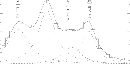
Figure 8: Portion of the spectrum from the compact brightening on September 13 showing the Fe xvii (347.85 Å) emission line and neighbouring lines. Fe xvii has a formation temperature of $\sim~{}5~{}\times~{}10^{6}~{}K$.

Table 4: Comparison between the parameters used in Equation 8 for Fe xvi (335.41 Å)/Fe xiv (334.18 Å).

Study	Log Ne	$a_{0}$	$a_{1}$	$a_{2}$	$a_{3}$
Brosius et al. (1996)	9.0	6.237	0.111	0.0087	0.0016
	10.0	6.217	0.108	0.0076	0.0018
Updated values	9.0	6.259	0.111	0.0105	0.0015
	10.0	6.240	0.108	0.0097	0.0015

3.4 Electron Pressures

The pressure maps in the bottom row of Fig. 5 follow a similiar behaviour to that seen in the density. Values for the pressure in the high density core of the active region remain $\sim$10¹⁶ K cm^-3 from September 10–13 and drop to 4$\times$10¹⁵ K cm^-3 on September 14, again not taking into account the effects of the brightening. Similar to the average electron density, the average pressure varied by $\sim$30 per cent between September 10–14 (see the values presented in Table 3 and Fig. 6).

3.5 Power Balance

The steady-state energetics of a coronal loop can be expressed as,

$$E_{H}=E_{R}+E_{C}+E_{F}~{}~{}{\rm~{}ergs~{}cm^{-3}~{}s^{-1}},$$ (9)

where $E_{R}$ is the total radiative losses of the plasma, $E_{C}$ is the thermal conductive flux, $E_{F}$ is the energy lost due to mass flows, and $E_{H}$ is the energy required to balance these losses (e.g. Antiochos & Sturrock 1982, Bradshaw & Mason 2003). The radiative loss term, $E_{R}$, in Equation (9) can be written in terms of the electron density, $N_{e}$, and the radiative loss function, $\Lambda(T_{e})$,

$$E_{R}=-N_{e}^{2}\Lambda(T_{e})~{}~{}{\rm~{}ergs~{}cm^{-3}~{}s^{-1}}.$$ (10)

The radiative loss function is usually approximated by analytical expressions of the form $N_{e}^{2}\chi T_{e}^{\alpha}$ (Cook et al., 1989). While this method is simple to implement computationally, it does not capture accurately the fine-scale structure of the radiative loss function. A more appropriate technique is used here, which relies on interpolating the values obtained from chianti, using the coronal abundances of Feldman (1992) and the ionization balance calculations of Mazzotta et al. (1998). The choice of coronal abundances was motivated by recent work by Del Zanna & Mason (2003) who show that low FIP elements in active regions have abundances which are coronal.

Assuming classical heat conduction along the magnetic field, the conductive flux can be expressed as,

$$E_{C}=\frac{d}{ds}\left[-\kappa T_{e}^{5/2}\frac{dT_{e}}{ds}\right]~{}~{}{\rm~{}ergs~{}cm^{-3}~{}s^{-1}},$$ (11)

where the thermal conductivity is $\kappa=0.92\times 10^{-6}~{}~{}{\rm ergs~{}s^{-1}~{}cm^{-1}~{}K^{-7/2}}$ (Spitzer, 1962), $T_{e}$ is the electron temperature. Various approximations for Equation (11) have been used in previous studies: Aschwanden et al. (1999) used an expression that was heavily dependent upon the temperature gradient, $(dT/ds)^{2}$, in the study of active region loops, whereas Varady et al. (2000) used an approximation strongly dependent upon temperature, $T^{7/2}$, for post-flare loops. Here, we assume a semi-circular loop geometry and approximate Equation (11) by,

$$E_{C}=-\kappa T_{e}^{5/2}\frac{\Delta T_{e}}{(L/2)^{2}}~{}~{}{\rm~{}ergs~{}cm^{-3}~{}s^{-1}},$$ (12)

where $\Delta T_{e}$ is the difference in the maximum and minimum temperatures given in Section 3.3, and $ds$ is approximated by $L/2$. This approximation is therefore not overly dependent on temperature or the temperature gradient, but acts as a balance between the approximations of Aschwanden et al. (1999) and Varady et al. (2000).

The energy losses due to mass motions of the plasma, $E_{F}$, can be expressed as a sum of the kinetic energy and the internal energy of the plasma,

$$E_{F}=\frac{d}{ds}\left[v\left(\frac{1}{2}\rho v^{2}+\frac{5}{2}N_{e}k_{B}T_{e}\right)\right]~{}{\rm~{}ergs~{}cm^{-3}~{}s^{-1}},$$ (13)

where $v$ is the flow velocity of the plasma, and $ds$ is again approximated to be the loop half-length ($L/2$). Line-of-sight velocities at the core of the active region were found to be $\sim$10 km s^-1 which is consistant with Brynildsen et al. (1999) who detected flow speeds of $\sim$15 km s^-1 also using CDS. Using these velocity values, as well as typical parameters from Table 3, the mass loss term was found to be $\sim$10²⁴ ergs s^-1. Energy losses due to mass motions can therefore be considered negligible compared to radiative losses.

Figure 9: The radiative, conductive, and mass losses, and the heating rate for NOAA 10103 for September 10–14.

In order to compare the work described in this paper with that of Fisher et al. (1998), Parker (1983), and others, Equation (9) has been integrated over the volume of the active region, and expressed as a power balance equation:

$$P_{H}=P_{R}+P_{C}+P_{F}~{}~{}{\rm~{}ergs~{}s^{-1},}$$ (14)

where $P_{R}$, $P_{C}$, and $P_{F}$ are the power lost due to radiation, conduction, and mass flows, respectively. $P_{H}$ is then the heating rate required to balance these losses.

Using the active region properties detailed in Table 3, the radiative, conductive, and mass flow losses were then calculated using Equations (10), (12), and (13). These results, together with the heating rate calculated using Equation (14), are presented in Table 3 and Fig. 9. Due to the difficulty in correlating emission seen in CDS with a particular magnetic flux concentration, the region’s average properties were used for comparision with MDI. The second panel down of Fig. 9 also shows how the conductive flux values depend on how Equation (11) is approximated. In each case, the conductive losses are found to be much less than the radiative losses. Indeed, the average radiative losses ($\langle P_{R}\rangle\sim 3\times 10^{25}$ ergs s^-1) are found to exceed both the conductive losses ($\langle P_{C}\rangle\sim 2\times 10^{24}$ ergs s^-1) and the mass flow losses ($\langle P_{F}\rangle\sim 4\times 10^{24}$ ergs s^-1) by approximately an order of magnitude. Aschwanden et al. (2000) also found an order of magnitude difference between the radiative and conductive losses in coronal loops despite the actual values being somewhat lower than those found here due to the insensitivity of EIT filter ratio techniques. As can be seen from Fig. 9, the heating rate falls by close to a factor of 5 between September 10 and 14 and is not significantly affected by whichever conductive loss equation is used.

The top panel of Fig. 10 shows the heating rate as a function of the total unsigned magnetic flux. A least-squares fit to the non-flaring data (i.e., neglecting the high density plasma of September 13) yielded a power-law of the form $P_{H}\sim\Phi_{tot}^{\gamma}$, where $\gamma=0.81\pm 0.32$. Power-laws with slopes of 1 and 2 from Equations (1) and (3) are also shown for comparison. The bottom panel of Fig. 10 shows how this relationship varies when densities from the core and the boundaries of the active region as well as from the quite solar corona (see Fig. 6) are used instead of average values. This wide range of $N_{e}$ shows that ${\gamma}$ varies from 0.2 in the quiet-Sun to 1.5 at the core of the region. It can therefore be concluded that average values of these parameters are a reasonable representation of the entire active region.

Figure 10: Top Panel: Plot of $P_{H}$ versus $\Phi_{tot}$ for five days of MDI and CDS observations. Also shown is a least-squares fit to the non-flaring data together with power-laws with slopes of 1 and 2 from the theoretical predictions. Bottom Panel: Plot of $P_{H}$ versus $\Phi_{tot}$, where $P_{H}$ has been calculated using non-flaring core (dotted line), boundary (dashed line), and quiet-Sun (dot-dashed line) parameters from Fig. 6.

4 DISCUSSION AND CONCLUSIONS

A detailed study of an evolving active region has been described using measurements from several instruments onboard SOHO. The region was observed to decay in size and complexity as it passed from close to the central meridian on September 10, to close to the west limb on September 14. In the photosphere, the total sunspot area fell by close to a factor of 2, while the total magnetic flux fell by approximately a factor of 6. In the corona, the average electron density, temperature, and pressure all showed similar decreases in value, which is to be expected considering that the plasma in the corona traces out field lines which are ultimately rooted in the photosphere. These results are of consequence to efforts in understanding active region evolution and the relationship between the photosphere and corona of solar active regions (e.g., Abbett & Fisher 2003; Ryutova & Shine 2004).

In addition to studying active region evolution, CDS and MDI were used to investigate the power-law relationships predicted by theoretical models of the corona. Mandrini et al. (2000) also investigated theoretical scaling laws using magnetic field extrapolations from both vector and longitudinal magnetograms, in light of the work of Klimchuk & Porter (1995). They concluded that models involving the gradual stressing of the coronal magnetic field are in better agreement with the observational contrains than are wave heating models. This same general conclusion was also reached by Démoulin et al. (2003) using photospheric and coronal measurements from MDI and Yohkoh. Unfortunately these studies relied on broad-band filter ratios to determine electron temperatures and densities; the difficulty associated with making such measurements is clear from the contradictory results of Priest et al. (1998), Aschwanden (2001), and Reale (2002), who also investigated coronal loop heating models using filter ratios from Yohkoh/SXT.

The analysis presented in this paper, on the other hand, is based on well understood line ratio techniques, which offer a less ambiguous determination of plasma properties. With this in mind, the power-law relationship between the total heating rate and the total unsigned magnetic flux ($\Phi_{tot}$) was determined, finding a relationship of the form $P_{H}\sim\Phi_{tot}^{0.81\pm 0.32}$. Fisher et al. (1998) compared the X-ray luminosity (which was assumed to be some fraction of the total heating power) to active region vector magnetograms, finding a similar power-law relation of $L_{X}\sim\Phi_{tot}^{1.19}$. The result of Fisher et al. (1998) suggests a “universal” relationship between magnetic flux and the amount of coronal heating, regardless of the age or complexity of the active region. A similar relationship of $L_{X}\sim\Phi_{tot}^{0.9}$ was found using statistical samples of late-type stars (Schrijver, 1987). The results of this paper therefore lend further observational evidence that active regions are heated by magnetically-associated waves, rather than multiple nanoflare-type events.

References

- Abbett & Fisher (2003) Abbett, W. P., Fisher, G. H. 2003, ApJ, 582, 475.
- Antiochos & Sturrock (1982) Antiochos, S. K., & Sturrock, P. A. 1982, ApJ, 254, 343
- Aschwanden et al. (1999) Aschwanden, M. J., Newmark, J. S., Delaboudinière, J. P., Neupert, W. M., Klimchuk, J. A., Gary, G. A., Portier-Fozzani, F., & Zucker, A. 1999, ApJ, 515, 842
- Aschwanden et al. (2000) Aschwanden, M. J., Alexander, D., Hurlburt, N., Newmark, J. S., Neupert, W. M., Klimchuk, J. A., & Gary, G. A. 2000, ApJ, 531, 1129A
- Aschwanden (2001) Aschwanden, M. J. 2001, ApJ, 559, L171
- Aschwanden et al. (2001) Aschwanden, M. J., Schrijver, C. J., & Alexander, D. 2001, ApJ, 550, 1036
- Berger & Lites (2003) Berger, T. E., & Lites, B. W. 2003, Sol. Phys., 213, 213
- Bradshaw & Mason (2003) Bradshaw, S. J., & Mason, H. E. 2003, A&A, 401, 699
- Brosius et al. (1996) Brosius, J. W., Davila, J. M., Thomas, R. J., & Monsignori-Fossi, B. C. 1996, ApJ, 106, 143
- Browning, Sakuria, & Priest (1986) Browning, P. K., Sakuria, T., & Priest, E. R. 1986, A&A, 158, 217
- Brynildsen et al. (1999) Brynildsen, N., Maltby, P., Brekke, P., Haugan, S. V. H., & Kjeldseth-Moe, O. 1999, Sol. Phys., 186, 141
- Cook et al. (1989) Cook, J. W., Cheng, C.-C., Jacobs, V. L., et al. 1989, ApJ, 338, 1176
- Dere et al. (1997) Dere, K. P., Landi, E., Mason, H. E., Monsignori-Fossi, B. C., & Young, P. R. 1997, A&AS, 125, 149
- Del Zanna & Mason (2003) Del Zanna, G., & Mason, H. E. 2003, A&A, 406, 1089
- Démoulin et al. (2003) Démoulin, P., van Driel-Gesztelyi, L., Mandrini, C. H., Klimchuk, J. A., Harra, L. 2003, ApJ, 454, 499
- Edlen (1937) Edlen, B. 1937, Z. Phys., 104, 407
- Feldman (1992) Feldman, U. 1992, Phys. Scripta, 46, 2002
- Fisher et al. (1998) Fisher, G. H., Longcope. D. W., Metcalf, T. R., & Pevtsov, A. A. 1998, ApJ, 508, 885
- Freeland & Handy (1998) Freeland, S. L., & Handy, B. N. 1998, Sol. Phys., 182, 497
- Gallagher et al. (2001) Gallagher, P. T., Phillips, K. J. H., Lee, J., Keenan, F. P., & Pinfield, D. J. 2001, ApJ, 558, 411
- Green et al. (2003) Green, L. M., Démoulin, P., Mandrini, C. H., & van Driel-Gesztelyi, L. 2003, Sol. Phys., 215, 307
- Gurman et al. (1974) Gurman, J. B., Withbroe, G. L. , & Harvey, J. W. 1974, Sol. Phys., 34, 105
- Harrison et al. (1995) Harrison, R. A., et al. 1995, Sol. Phys., 162, 233
- Klimchuk & Porter (1995) Klimchuk, J. A., & Porter, L. J. 1995, Nature, 377, 131
- Mandrini et al. (2000) Mandrini, c. H., Démoulin, P., & Klimchuk, J. A. 2000, ApJ, 530, 999
- Mazzotta et al. (1998) Mazzotta, P., Mazzitelli, G., Colafrancesco, S., & Vittorio, N. 1998, A&AS, 133, 402
- Parker (1983) Parker, E. N. 1983, ApJ, 264, 642
- Parker (1988) Parker, E. N. 1988, ApJ, 330, 474
- Priest et al. (1998) Priest, E. R., Foley, C. R., Heyvaerts, J., Arber, T. D., Culhane, J. L., & Acton, L. W. 1998, Nature, 393, 545
- Reale (2002) Reale, F. 2002, ApJ, 580, 566
- Ryutova & Shine (2004) Ryutova, M., & Shine, R. 2004, ApJ, 606, 571R
- Scherrer et al. (1995) Scherrer, P. H., et al. 1995, Sol. Phys., 162, 129
- Schrijver (1987) Schrijver, C. J. 1987, A&A, 180, 241
- Spitzer (1962) Spitzer, L. 1962, Physics of Fully Ionized Gasses (New York: Interscience)
- Thompson (1999) Thompson, W. T. 1999, CDS Software Note No. 53
- van Driel-Gesztelyi et al. (2003) van Driel-Gesztelyi, L., Démoulin, P., Mandrini, C. H., Harra, L., & Klimchuk, J. A. 2003, ApJ, 586, 579
- Varady et al. (2000) Varady, M., Fludra, A., & Heinzel, P. 2000, A&A, 355, 769
- Warren & Winebarger (2003) Warren, H. P., & Winebarger, A. R. 2003, ApJ, 596, L113