Evolution of 1612 MHz Maser Emission in Expanding Circumstellar Shells

Abstract

Observations show that 1612 MHz masers of OH/IR stars can fade on a timescale of a decade. This fading is probably associated with the switch from rapid mass loss, which is ultimately linked with an internal He-shell flash, to the much slower mass loss supported by more quiescent conditions. We study the observed maser decay with a composite computational model, comprising a time-dependent chemical model of the envelope, and a radiation transfer model which provides the maser pumping. Our combined model is able to reproduce the rapid decay of maser intensity, following a sudden drop in the stellar mass-loss rate. The explanation for the rapid fall in maser emission is not a fall in the OH number density, or the kinetic temperature in the inverted layers, but the loss of a radiative pump route which carries population from level $1$ to level $4$ via levels $16$, $15$ and $11$. The loss of these pump routes is a result, in turn, of a greatly reduced energy density of $53$ $\mu$m radiation.

1 Introduction

When discovered in May 1988 the 1612 MHz masers of IRAS 18455+0448 had a classic, two-horned, morphology with a peak intensity for its strongest maser of 2.1 Jy. However, these had faded to a solitary 110 mJy maser by July 1998, whose subsequent exponential decline is documented by Lewis, Oppenheimer & Daubar [2001], until it became completely undetectable in January 2001. We thus see that the masers of an apparently normal OH/IR star can fade by a factor of more than a thousand in just 13 years. Nor is 18455+0448 unique, as the 1612 MHz masers of three other OH/IR stars from the Arecibo sample have similarly disappeared, while those of a fifth, FV Boo, are declining exponentially, and so should disappear within the next 2-4 years [2002].

These five instances of ‘dead’ OH/IR stars come from a complete sample of 328 that had $>$100 mJy masers when first detected at Arecibo. As such they imply an average duration, $\tau_{1612}$ , for $1612$ MHz emission of $328\times 14/5\sim 920(+1133,-693)$ yr for a general member of the population of OH/IR stars in the Arecibo $(0\degr\leq\delta\leq 38\degr)$ sky. But these dead stars are more particular than that as they all have rather blue IR colours and small, $<12$ km s^-1, expansion velocities. When death statistics are calculated for the $112$ objects in the sample with similar parameters, the maser lifetime is found to be $\tau_{1612}=112\times 14/5\sim 314(+387,-97)$ yr: the 1612 MHz masers exhibited by this subset of OH/IR stars only have a transient existence.

We can assimilate these observational results into our understanding of the evolution of AGB stars, by recalling the models by Wood & Vassiliadis [1992], which show that a brief, copious, mass-loss regime first occurs while an AGB star is radiating away the extra energy it generates during a He-shell flash. This fillip to the stellar luminosity lasts $\sim 500$ yr [1981]. But this causality does match the brevity of the $1612$ MHz emission phase, and does imply that the phase will recur whenever the star passes through a He-shell flash. Moreover, in the case of low-mass progenitor stars, the copious mass-loss phase is likely to dominate mass-loss while they are on the AGB, as these stars may never be luminous enough to support much mass-loss otherwise. The diverse observational data supporting this scenario, which comes from studies of high-latitude OH/IR stars, is discussed by Lewis [2001].

Until now models of the radial distribution of molecules in the circumstellar shells of AGB stars have assumed a constant mass-loss rate over time-scales of order $10000$ yr (Huggins & Glassgold [1982]; Netzer & Knapp [1987]). These models are appropriate when discussing most of the classic OH/IR stars with massive progenitors, which fall near the Galactic Plane, as these stars do eventually reach the copious mass-loss phase while on the luminosity ascent towards a thermal pulse. They also have periods of order $1000-2000$ d and expansion velocities of $>12$ km s^-1. By contrast the low-mass and/or transient OH/IR stars all have periods of less than $700$ d, and usually have expansion velocities of less than $12$ km s^-1. There is thus clearly a need to revisit the models for the distribution of molecules about O-rich AGB stars, to incorporate the transient aspects of their shells. Our objective here is to determine what properties these shells must have to reproduce the brevity of their $1612$ MHz masers and the speed with which normal $1612$ MHz masers can fade away.

2 Deriving the Radial OH Profile

The OH found in OH/IR envelopes is assumed to be produced predominantly from the photodissociation of H₂O. The abundance of OH at any time and position is controlled by subsequent photodissociation of OH itself. The UV photons in these reactions are assumed to be entirely of interstellar origin. Two-body reverse reactions are included, though they are endothermic and therefore relatively unimportant for the case considered in this paper, owing to the low temperatures in the region where UV optical depth is low enough to give significant photodissociation rates. Over time the above reactions lead to a classic hollow shell OH distribution [1981, 1987]. In order to deal with a brief superwind episode, as opposed to continuous mass loss, a time-dependent model was constructed, involving a series of runs, for gas emitted at different times during the superwind episode. The ejected envelope is thus modelled as a series of concentric spherical shells (depth elements) of thickness $v\delta t$ emitted at time intervals $\delta t$ and drifting away from the central star at constant terminal speed $v$ ($10$ km s^-1 for the present work). The gas kinetic temperature, $T_{gas}$, is modelled by a simple power-law function. At the time of shell detachment, the gas temperature is given by $T_{gas}=3.2\times 10^{14}r_{cm}^{-0.79}$, where $r_{cm}$ is the radius in cm [1986]. The change in OH number density of each depth element over each $\delta t$ is calculated using an integration package by Gear [1971].

From the time when the superwind episode is terminated, no further depth elements are produced, and those already emitted continue to drift away forming a detached circumstellar envelope. This envelope becomes cooler and more diffuse, causing the OH abundance to fall, as (i) dissociation rates are rising with falling optical depth and (ii) the H₂O from which the OH forms is no longer being supplied to the photodissociation region.

Though the interstellar UV flux is assumed isotropic, the optical depth out of the envelope (due mainly to dust) varies with direction. Therefore, in order to estimate photodissociation rates, it is necessary to find the integral over direction of a direction-dependent flux. In steady state models it is common to estimate an average attenuation as a function of the outward radial value, $\theta=0$, for example Morris & Jura [1983]. In the case covered here we have opted for a more accurate treatment (albeit using a very simplified density structure) due to UV coming from previously heavily shielded directions with $\theta>\pi/2$ becoming more important as the envelope detaches (in addition it was thought that the more accurate approach would give extra flexibility if, for example, it were desired at some point to vary the mass loss rate during the superwind episode instead of switching it on then off after a certain time). The gas to dust mass ratio was set at 100 and the UV absorption spectrum of dust taken from Massa & Savage [1989]. We note that the dust absorption spectrum used in this part of the computational model is observationally based, and is different to the model used by the maser pumping code (see Section 3). However, since the main spectral region of importance in the envelope code is the ultraviolet, while the important region for maser pumping is the far infra-red, the two models are not contradictory. The dust to gas mass ratio is $0.01$ in both models.

For the abundances adopted here, dust makes the dominant contribution to UV optical depth, though continuum shielding by H₂O and OH was included, using cross section data from van Dishoeck & Dalgarno [1984]. For details of how UV attenuation was calculated for a given column density, see Howe & Rawlings [1994]. For each run, column densities were calculated at the beginning of each time step for 6 directions relative to the outward radial ($\theta=0$) between $\theta=0$ and $\theta=\pi$, the chosen directions being dictated by the Gaussian quadrature method used to integrate the directional flux. To avoid undue weighting of directions with $\theta\sim\pi/2$, the integration variable was not $\theta$ itself, but the solid angle subtended by $\theta$. The total column in a given direction was estimated by adding that of each depth element intercepted by that line of sight, assuming each absorbing species to have a uniform fractional abundance within that depth element, such that its number density has an inverse square relation with distance from the central star (which can be integrated analytically between the points where the line of sight enters and leaves the depth element). Because the abundances of OH and H₂O are results rather than inputs of the model, the inclusion of continuum shielding by these species means that the model is iterated several times, starting with dust shielding alone, until convergence is achieved. Once photorates have been found for the beginning of each timestep, for each depth element, the rate used to calculate abundances during the timestep was a linear interpolation between the initial rate and that at the start of the next step (this was easily achieved given the fact that the model was already iterative for the shielding calculation).

3 The OH Pumping Model

We use a model based on the accelerated lambda iteration (ALI) method [1985] with modifications necessary to make it applicable to molecular line studies [1994]. The modified code, multimol, has already been successfully applied to OH absorption [1994], to megamaser emission [1995] and to studies of OH maser emission in star-forming regions [2001]. Here, we combine the chemical model described in Section 2 with multimol to produce a time-series of OH pumping models that follow the evolution of a circumstellar shell from the time that the shell detaches from the host star to, at most, $1000$ yr later.

We adopt the slab version of multimol to study OH, rather than the spherical version [1998] because the former has far-infrared (FIR) line overlap built into the code whilst the latter does not. FIR line overlap is vital to OH pumping schemes, so we chose to model this accurately and accept some deficiencies in the geometry, rather than the other way about. Some quantities required geometric corrections because the slab model was chosen; these are discussed below. The OH-containing shell, of which the $1612$ MHz maser emitting zones form a subset, is thin compared to the shell radius in all cases except for the model with the lowest mass-loss rate. Except in this case, the use of a slab geometry should not introduce very significant errors into the results.

Individual slabs for each timestep were developed as follows: The chemical model, discussed in Section 2, has linearly-spaced slabs, ordered outward in radius from the star. However, multimol requires logarithmically spaced layers ordered inwards from the outer edge of the envelope. Therefore, a service routine reversed the row order of the file, before fitting the data with a natural cubic-spline, which was then interpolated at the required logarithmic points, according to the formula,

$$z_{k}=z_{1}(z_{M}/z_{1})^{k/M}$$ (1)

where $z_{k}$ is the depth of layer $k$, and there are $M$ layers altogether in the slab. The spline and interpolation routines were taken from Press et al. [1996].

Other inputs to multimol comprised a set of energy levels and Einstein A-values for OH [1977] and collisional rate-coefficients for OH with molecules of ortho- and para-hydrogen [1994]. A dust model (see Section 3.1) was used to compute the continuum over the wavelength range appropriate for the pumping lines of OH, but there was no direct contribution from the central star. The models discussed here used the $36$ lowest-lying hyperfine energy levels of OH. Competitive propagation of polarized masers involving magnetic hyperfine splitting [1995] was not treated here. Following successful convergence of multimol the solution is exact for the geometry employed and the set of FIR transitions which form the radiation-transfer solution. We note that, given the comments above about the geometry, the solutions are only approximate for the spherical case. We also note that we keep a separation of pump and maser, such that the microwave transitions, whether masing or not, do not form part of the NLTE radiation-transfer solution which controls the molecular population: we only calculate unsaturated gain-coefficients in the microwave transitions, based on inversions fixed by the FIR transitions and collisional processes. The Monte-Carlo radiative transfer solution by Spaans & van Langevelde [1992] is more appropriate to the geometry of the situation, and includes saturation. However, the model in the present work includes much more detail regarding the OH molecule, its collisions with H₂, its interaction with radiation, and the role of dust.

3.1 The Dust Model

The dust model used by the ALI computer code is based on theoretical calculations of absorption and scattering efficiencies for spherical grains by Laor and Draine [1993] and Draine and Lee [1984]. These efficiencies are derived from the tables of optical constants in Draine [1985]. The optical constants were tabulated for silicate and graphite, but for the purposes of this work, we have made the silicate fraction overwhelming, as we are dealing with oxygen-rich stars, which we assume do not produce carbon dust. At all modelled points in the envelope, we assume a constant dust mass fraction of 1%. The size of dust grains was allowed to vary from $1$ nm up to $10$ $\mu$m, following a power-law spectral index equal to $-3.5$. In this respect, the model resembles MRN [1977] dust, with an extended size range and no carbon component. For the spectra of several MRN-like models, and comparison with other theoretical and observational dust ‘laws’, see Gray [2001]. In particular, the parameters of the dust model in the present work are very similar to the model ‘E’ in Gray [2001], but without the graphite.

The dust model described here was only used to provide a continuum in the spectral vicinity of the OH pumping lines (from about $10$ to $200$ $\mu$m) with most of these lines lying in the far infra-red. The dust absorption spectrum was not used to compute dynamical effects, via radiation pressure, nor to calculate dust temperatures. The dust temperature was instead related to the gas kinetic temperature via simple empirical formulae, which could be changed from model to model (see Section 4). In most cases the formula used was $T_{dust}=max(25,T_{gas}-25)$, where $T_{dust}$ and $T_{gas}$ are the dust and gas temperatures in Kelvin. The minimum dust temperature was used to represent the value which can be maintained by typical interstellar irradiation [1978].

4 Results

Our model, comprising the hydrodynamic and photo-chemical model of the detached envelope (see Section 2) and the radiation transfer code discussed in Section 3, was run for a series of stellar mass-loss rates. These rates refer to values of $\dot{M}$ prior to a time when the envelope detaches, when the mass-loss rate is assumed to fall to a negligibly low value. Seven versions of the model were run, with mass-loss rates, $\dot{M}$, ranging from $1.0\times 10^{-6}$ M_⊙ yr^-1 up to $1.0\times 10^{-4}$ M_⊙ yr^-1. We show the distribution of the number densities of molecular hydrogen and OH as a function of radius in the shell in Figure 1. Graphs are plotted for three mass-loss rates, including the lowest and highest used. All data are plotted at the time of shell detachment. An additional model was run at a mass-loss rate of $1.0\times 10^{-4}$ M_⊙ yr^-1, but a longer ($600$ yr) elapsed time before shell detachment. The elapsed time was $300$ yr in all other cases.

We note that the model run at a mass-loss rate of $1.0\times 10^{-6}$ M_⊙ yr^-1 has a significant abundance of OH deep inside the envelope. The accuracy of the slab model as an approximation to spherical geometry is therefore poor in this case, and to a lesser extent in the model at $3.0\times 10^{-6}$ M_⊙ yr^-1. Accuracy of the geometrical representation rises rapidly with mass-loss rate.

Figure 1: The variation, at shell detachment, of the number densities of H₂ and OH, as a function of radius in the shell. Data are plotted for three mass-loss rates: $1.0\times 10^{-4}$ M_⊙ yr^-1 (solid line), $1.0\times 10^{-5}$ M_⊙ yr^-1 (long dashes) and $1.0\times 10^{-6}$ M_⊙ yr^-1 (short dashes).

In each model the time begins at zero and, prior to shell detachment, the model star loses mass at the rate applicable to that version. At shell detachment, usually $t=300$ yr, the mass-loss rate falls to zero, and the circumstellar shell becomes progressively more hollow. This corresponds to the end of a superwind phase in the language of Section 2. From detachment onwards, the unsaturated maser gain is calculated at each timestep. The calculations were continued until the gain at $1612$ MHz had clearly fallen into absorption (indicated here, and in Tables 1-7, by negative values of $\Gamma$). This only took more than $100$ yr in the one-off model in which shell detachment occurred at $600$ yr. Detached solutions were available to continue calculations until $t=1500$ yr, had this been necessary. In Tables 1-7, we show the variation of the integrated gain through the shell in the four ground-state lines of OH as a function of time for seven mass-loss rates and shell detachment at $300$ yr. Times prior to shell detachment are not shown. Where information for times is missing, the radiative transfer code did not reach an acceptable solution within a reasonable number ($250$) of iterations.

Table 1: $\dot{M}=1.0\times 10^{-6}$ M_⊙ yr^-1

Time	$\Gamma_{1720}$	$\Gamma_{1667}$	$\Gamma_{1665}$	$\Gamma_{1612}$
(yr)
300	-19.827	-84.607	-36.591	3.107
310	-16.127	-92.746	-41.219	-2.421
320	-15.085	-102.321	-46.477	-5.579
340	-16.421	-122.991	-61.982	-9.640
360	-15.170	-131.971	-66.790	-12.894
380	-12.656	-133.398	-68.372	-15.838

Table 2: $\dot{M}=3.0\times 10^{-6}$ M_⊙ yr^-1

Time	$\Gamma_{1720}$	$\Gamma_{1667}$	$\Gamma_{1665}$	$\Gamma_{1612}$
(yr)
300	-26.345	-62.275	-22.615	14.900
310	-27.539	-87.366	-42.524	9.325
320	-28.104	-100.424	-53.198	6.306
330	-26.448	-109.520	-59.880	2.303
340	-25.634	-117.503	-65.666	-0.555
360	-24.903	-132.800	-75.380	-4.928
370	-25.061	-140.388	-79.799	-6.496
380	-24.657	-146.187	-84.244	-8.433
390	-23.798	-152.630	-88.136	-10.786

Table 3: $\dot{M}=1.0\times 10^{-5}$ M_⊙ yr^-1

Time	$\Gamma_{1720}$	$\Gamma_{1667}$	$\Gamma_{1665}$	$\Gamma_{1612}$
(yr)
300	-11.324	2.603	16.831	14.977
310	-17.383	-24.675	-5.892	13.461
320	-20.417	-43.418	-21.057	11.380
330	-22.290	-58.811	-32.998	9.155
340	-23.219	-70.508	-41.848	7.014
350	-23.640	-81.343	-49.657	4.670
360	-23.847	-91.470	-56.723	2.339
370	-24.051	-100.989	-63.243	-0.002

Table 4: $\dot{M}=1.5\times 10^{-5}$ M_⊙ yr^-1

Time	$\Gamma_{1720}$	$\Gamma_{1667}$	$\Gamma_{1665}$	$\Gamma_{1612}$
(yr)
300	1.690	36.579	35.366	9.446
310	-3.956	16.069	19.131	9.567
320	-7.784	-0.829	5.779	8.846
330	-10.685	-16.034	-5.735	7.755
340	-12.537	-28.310	-14.824	6.426
350	-14.086	-40.842	-23.576	4.832
360	-15.044	-52.797	-31.550	2.867
370	-15.613	-62.601	-37.830	1.091
380	-15.869	-74.144	-44.734	-1.316
390	-15.581	-85.750	-51.234	-4.193
400	-15.361	-94.955	-56.277	-6.444

Table 5: $\dot{M}=2.0\times 10^{-5}$ M_⊙ yr^-1

Time	$\Gamma_{1720}$	$\Gamma_{1667}$	$\Gamma_{1665}$	$\Gamma_{1612}$
(yr)
300	3.998	34.676	32.683	6.391
310	-0.718	19.678	20.868	7.077
320	-4.279	5.940	9.924	6.902
330	-7.243	-7.214	-0.307	6.379
340	-9.240	-18.131	-8.663	5.492
350	-11.114	-29.774	-17.060	4.393
360	-12.407	-41.079	-24.903	2.862
370	-13.285	-50.386	-31.138	1.459
380	-13.968	-61.842	-38.314	-0.566
390	-14.059	-73.284	-44.983	-3.080
400	-14.168	-82.713	-50.375	-5.096

Table 6: $\dot{M}=3.0\times 10^{-5}$ M_⊙ yr^-1

Time	$\Gamma_{1720}$	$\Gamma_{1667}$	$\Gamma_{1665}$	$\Gamma_{1612}$
(yr)
300	6.027	21.353	23.724	1.090
310	2.081	12.316	16.850	2.657
320	-1.427	2.831	8.952	3.531
330	-4.511	-7.737	0.583	3.749
340	-6.849	-17.022	-7.097	3.537
350	-8.912	-26.159	-14.169	3.172
360	-10.791	-37.057	-22.457	2.182
370	-12.112	-45.578	-28.792	1.289
380	-13.307	-54.540	-35.215	0.204
390	-14.207	-66.223	-43.199	-1.790
400	-14.869	-75.468	-49.340	-3.383

Table 7: $\dot{M}=1.0\times 10^{-4}$ M_⊙ yr^-1

Time	$\Gamma_{1720}$	$\Gamma_{1667}$	$\Gamma_{1665}$	$\Gamma_{1612}$
(yr)
300	3.893	2.485	4.595	-2.698
310	4.424	1.628	4.787	-3.285
320	4.115	1.182	4.530	-3.077
330	3.827	-1.299	3.324	-3.307
340	2.593	-3.071	1.424	-2.649
350	1.966	-6.396	-0.580	-2.792
360	0.328	-10.805	-4.382	-2.405
370	-0.777	-14.527	-7.335	-2.303

The general trend from the tables is that the gain of the $1612$ MHz masers decays to absorption on a timescale of a few decades after shell detachment. Apart from the case of the highest mass-loss rate (Table 7) there are always $1612$ MHz masers present at the time of shell detachment. The extra model, with shell detachment at $600$ yr, does have $1612$ MHz masers present at the time of detachment: in this case the initial integrated gain of $1.728$, rises to a maximum of $5.211$ at $40$ yr after detachment, followed by a decay to absorption lasting an additional $80$ yr. For the models with shell detachment at $300$ yr, the initial masers are strongest between mass-loss rates of $3.0\times 10^{-6}$ M_⊙ yr^-1 and $1.0\times 10^{-5}$ M_⊙ yr^-1. At both these values of $\dot{M}$ the maser intensity at $t=300$ yr would in practice be limited by saturation. The longest-lasting $1612$ MHz masers are at $\dot{M}=3.0\times 10^{-5}$ M_⊙ yr^-1, where they remain inverted until $80$ yr after shell detachment. Except at $\dot{M}=1.0\times 10^{-4}$ M_⊙ yr^-1, any masers initially present in the other three lines decay substantially more quickly than those at $1612$ MHz. However, for the main lines, the current model ignores masers generated deep within the shell (in a zone shared with water masers, for example Richards et al. [2002]) where there would be a shock source of OH, rather than the source generated by interstellar UV photodissociation which is used in the present work.

We proceed to compare the decay times of our model $1612$ MHz masers with the values obtained by Lewis et al. [2001] for IRAS 18455+0448, and by Lewis [2002] for FV Boo.

4.1 Model Parameters and Decay Times

Here we discuss the input parameters for the models discussed in Section 4. Parameters that were considered standard for all models are set out in Table 8. The thickness of the OH shell is the maximum found, corresponding to the smallest mass-loss rate of 10^-6 M_⊙ yr^-1. Typical values at higher mass-loss rates were considerably smaller. In all the models that were run to produce the data in Tables $1$-$7$, the dust temperature in the outer envelope was not allowed to fall below $25$ K, a value maintained by the interstellar radiation field [1978]. An additional test model was also run in which the dust temperature was linked only to the gas temperature, being offset from it by $-25$ K, with no minimum other than absolute zero. At a mass-loss rate of 10^-5 M_⊙ yr^-1, differences between the test model and the data in Table 3 were less than 5% in the worst case.

For the models in Tables $1$-$3$, $6$ and $7$, the value of the integrated gain coefficient at line-centre for the $1612$ MHz maser, as a function of time, is plotted in Fig. 2. The time origin is taken as the moment of shell detachment.

Table 8: Model Parameters

Parameter	Value	Unit
Shell depth	$8.13\times 10^{15}$	cm
Thickness of OH shell (max.)	$7.21\times 10^{15}$	cm
Number of depth points	82
OH levels modelled	36
Radiation angles	3
Velocity shift	0.0	km s-1
Microturbulent velocity	0.0	km s-1
Expansion velocity	10	km s-1
Dust temperatures	$max(T_{gas}-25,25)$	K

For each of the models which has a strong $1612$-MHz maser at the time of shell detachment, we compute a decay time, over which the unsaturated maser amplification falls to $1/2$ of its original value. The models considered in this way comprise Tables $1$-$6$. We note that in model $6$ there is a period of initial increase in amplification factor. In this case, we add the time to reach maximum ($30$ yr) to the decay time.

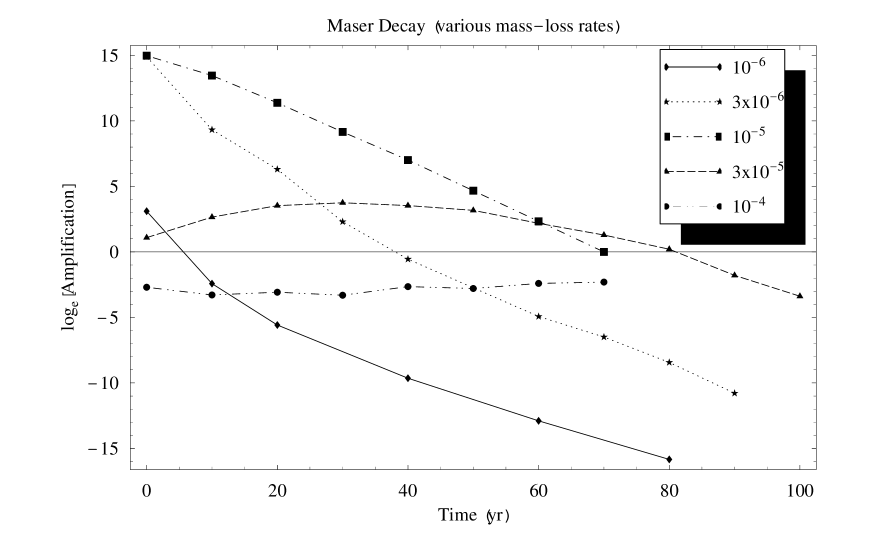
Figure 2: Decay of the line-centre maser gain as a function of time for model stars with five different mass-loss rates (in solar masses per year). Note that the amplifications given do not take saturation into account. Values of the logarithm above $\sim$10-11 would be about the maximum achieved under the limit of strong saturation,

In all cases, we assume that changes in the observed flux density of the $1612$-MHz maser result from a change in the pumping scheme, which reduces the maser gain coefficient. The observed fluxes are then proportional to total amplification factors in the maser column. We ignore saturation here, though the masers in Tables $2$ and $3$ would probably be partially saturated. Suppose we want to calculate the time taken for an observed flux density to fall to some fraction, $r$, of its value at the time of shell detachment. The fraction is given by

$$r=\frac{S_{\nu}(t)}{S_{\nu}(t_{0})}=\frac{A(t)}{A(t_{0})}$$ (2)

where $S_{v}(t)$ is a flux density, and $A(t)$ is a computed amplification factor. The amplification is given in terms of the overall integrated gain, $\Gamma$, of the model as $A(t)=\exp(\Gamma(t))$. Therefore the logarithm of $r$ is just given by the difference in the integrated gains at the two times, or

$$\ln r=\Gamma(t)-\Gamma(t_{0})$$ (3)

For small times, $t-t_{0}$, we can expand $\Gamma(t)$ in a Taylor series about $t=t_{0}$, and truncate at the linear term, leaving

$$\Gamma(t)\sim\Gamma(t_{0})+\left.\frac{d\Gamma}{dt}\right|_{t=t_{0}}(t-t_{0})$$ (4)

This can be used in eq.(3) to eliminate $\Gamma(t_{0})$, and supposing that we choose $r=1/2$, we can obtain an estimate of the ‘half-life’ of the maser decay as,

$$\tau_{1/2}=(t-t_{0})_{1/2}=\frac{-\ln 2}{(d\Gamma/dt)|_{t=t_{0}}}$$ (5)

If we approximate the differential as the finite difference between the initial time and the second computation ($10$ yr later), we find half-lives for maser decay of $1.25$ yr at a mass-loss rate of $10^{-6}$ M_⊙ yr^-1, falling slightly to $1.24$ yr at $3.0\times 10^{-6}$ M_⊙ yr^-1, and then rising to $4.57$ yr when the mass-loss rate reaches $10^{-5}$ M_⊙ yr^-1. For mass-loss rates larger than $10^{-5}$ M_⊙ yr^-1, the situation is complicated by an initial period of growth in maser amplification before the decay sets in. A naive method of calculating the decay time in these cases is to take the decay time from the peak. For example, at $3\times 10^{-5}$ M_⊙ yr^-1, the peak is reached after $30$ yr and, starting from this time, the half-life from eq.(5) is some $33$ yr. A more sophisticated analysis is to view the data in Tables $4$-$6$ as an intermediate case between the $10^{-4}$ M_⊙ yr^-1 shell, where not enough time has elapsed before shell detachment for $1612$ MHz OH masers to form, and the lower mass-loss rate cases, where decay of these masers begins immediately after shell detachment. The extra model in which the shell detaches after $600$ yr, as discussed in Section 4, shows that $1612$ MHz masers can form in envelopes with loss-rates of $10^{-4}$ M_⊙ yr^-1, given a longer episode of mass loss before detachment. It is therefore instructive to plot the decay of the $1612$ MHz masers in the three cases which have mass loss rates between $10^{-5}$ M_⊙ yr^-1 and $10^{-4}$ M_⊙ yr^-1 without the other models present (Fig. 3).

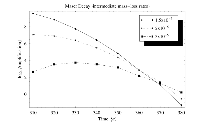
Figure 3: Decay curves for three models at mass loss rates between $10^{-5}$ M_⊙ yr^-1 and $10^{-4}$ M_⊙ yr^-1, showing the initial slow decay from the peak of each curve, followed by an approximately linear fall with time.

We can see from Fig. 3 that an inital slow decline from the peak, in all three cases, is followed by a roughly linear fall in $\Gamma$ with time. Basing the decay of the $1612$-MHz masers in the $3$ intermediate models on this linear section of the graph only, we find a much shorter half-life of $7.01$ yr for the $3\times 10^{-5}$ M_⊙ yr^-1 case. The linear section is taken to start twenty years after the peak, and to continue until the last positive value of $\Gamma$. Similar calculations yield $4.16$ yr for $1.5\times 10^{-5}$ M_⊙ yr^-1 and $5.64$ yr for $2\times 10^{-5}$ M_⊙ yr^-1. We note that the models with mass-loss rates of $10^{-5}$ M_⊙ yr^-1 and lower also exhibit quasi-linear declines of $\Gamma$ with time. These computational results compare to a decay time for the red peak of FV Boo of some $250-300$ d ($0.68-0.82$ yr).

We go on to consider the variation of the maser decay half-life, $\tau_{1/2}$, as a function of the mass-loss rate. For the mass-loss rates above $10^{-5}$ M_⊙ yr^-1, we use the values of the half-life computed from the quasi-linear region of Fig. 3. The relationship is plotted in Fig. 4.

Figure 4: The variation of the decay half-life of $1612$ MHz masers as a function of mass-loss rate.

For the remaining points, we compute half-lives based on all points in Fig. 2 up to, and including, the first point with a negative value of $\Gamma$. This rule yields values of $\tau_{1/2}$, for the mass loss rates of $1$, $3$ and $10\times 10^{-6}$ M_⊙ yr^-1, of $1.25$, $1.79$ and $3.24$ yr, respectively. For the models with mass-loss rates of $10^{-5}$ M_⊙ yr^-1 and lower, we find a linear relation between the half-life of decay and the mass-loss rate, which is

$$\tau_{1/2}=13.19+1.99\log_{10}(\dot{M}/(M_{\odot}\,yr^{-1}))\;\;{\rm yr}$$ (6)

A possible explanation for the change in the behaviour of the half-life at a mass-loss rate of $\sim 10^{-5}$ M_⊙ yr^-1 is that $300$ yr is sufficient for masers to become saturating for mass-loss rates lower than this, and at higher mass-loss rates the shell has not been undergoing a superwind loss for long enough to achieve saturation. This view is supported by the appearance of strong masers in the model run after $600$ yr of mass-loss for a loss rate of $10^{-4}$ M_⊙ yr^-1.

4.2 Position of Emitting Shells

Here we consider the zones in the envelope which contribute most to the maser output for Tables $1$-$7$. At the time of shell detachment, and for most of the models, the OH that sustains an inversion is divided into two layers: a very thin layer bordering the outer edge of the shell, and a deeper layer which is much thicker, although the inversions are smaller. As the mass-loss rate increases, the already thin outer layer becomes physically even thinner, though its inverted column density increases somewhat, whilst the deeper layer gets closer to the surface, and narrows. A very weakly inverted third emission layer develops for mass-loss rates above $3.0\times 10^{-5}$ M_⊙ yr^-1, but this contributes little to the maser output of the star. For all models, it is the second inverted layer which contributes the great majority of the maser output. The absorbing layer, found between this and the outer emission zone, can absorb anything from $\sim 10$ per cent to $100$ per cent of the maser emission. The outer emitting layer typically adds only a few per cent or less of the maser emission generated by the deeper emitting zone.

Table 9: Parameters of emitting and absorbing zones of the envelope at the time of shell detachment. Column densities given are the column densities per sublevel of OH molecules in the upper level of the 1612 MHz transition (level $3$) minus the corresponding column densities of OH, per sublevel, in the lower level of this transition (level $2$). This definition means that inverted column densities are positive; absorbing column densities are negative. The terms Zone 1 and Zone 2 refer to the outer and inner inverted layers respectively. Depths, $z$, are measured from the outer (ISM) surface of the envelope. $z_{out}$ for Zone 1 is zero in all cases.

$\dot{M}$	$z_{in}$ Zone 1	$z_{out}$ Zone 2	$z_{in}$ Zone 2	Zone 1 column	Interzone absorption	Zone 2 column
M⊙ yr-1	cm	cm	cm	cm-2	cm-2	cm-2
$1.0\times 10^{-6}$	$9.98\times 10^{12}$	$1.52\times 10^{15}$	$6.40\times 10^{15}$	$7.35\times 10^{10}$	$-8.39\times 10^{12}$	$2.76\times 10^{13}$
$3.0\times 10^{-6}$	$4.32\times 10^{12}$	$2.24\times 10^{14}$	$4.47\times 10^{15}$	$1.75\times 10^{11}$	$-4.27\times 10^{12}$	$7.15\times 10^{13}$
$1.0\times 10^{-5}$	$1.47\times 10^{12}$	$3.72\times 10^{13}$	$2.18\times 10^{15}$	$3.13\times 10^{11}$	$-2.94\times 10^{12}$	$6.23\times 10^{13}$
$1.5\times 10^{-5}$	$1.03\times 10^{12}$	$1.82\times 10^{13}$	$1.06\times 10^{15}$	$3.84\times 10^{11}$	$-1.47\times 10^{12}$	$3.42\times 10^{13}$
$2.0\times 10^{-5}$	$9.10\times 10^{11}$	$1.27\times 10^{13}$	$6.58\times 10^{14}$	$4.58\times 10^{11}$	$-2.42\times 10^{12}$	$2.27\times 10^{13}$
$3.0\times 10^{-5}$	$8.08\times 10^{11}$	$1.27\times 10^{13}$	$3.21\times 10^{14}$	$5.59\times 10^{11}$	$-2.88\times 10^{12}$	$9.26\times 10^{12}$
$1.0\times 10^{-4}$	$7.17\times 10^{11}$	$7.85\times 10^{12}$	$2.93\times 10^{13}$	$6.78\times 10^{11}$	$-2.80\times 10^{12}$	$8.25\times 10^{11}$

Table 10: As for Table 9, but for a time of $40$ yr after shell detachment. Note that for the lowest mass-loss rate, the deeper inverted layer has entirely disappeared, and absorption persists to the maximum depth of the model.

$\dot{M}$	$z_{in}$ Zone 1	$z_{out}$ Zone 2	$z_{in}$ Zone 2	Zone 1 column	Interzone absorption	Zone 2 column
M⊙ yr-1	cm	cm	cm	cm-2	cm-2	cm-2
$1.0\times 10^{-6}$	$1.82\times 10^{13}$	N/A	N/A	$8.19\times 10^{10}$	N/A	N/A
$3.0\times 10^{-6}$	$6.18\times 10^{12}$	$2.77\times 10^{15}$	$7.21\times 10^{15}$	$1.55\times 10^{11}$	$-1.37\times 10^{13}$	$1.86\times 10^{13}$
$1.0\times 10^{-5}$	$1.87\times 10^{12}$	$1.99\times 10^{14}$	$5.04\times 10^{15}$	$2.78\times 10^{11}$	$-6.80\times 10^{12}$	$3.67\times 10^{13}$
$1.5\times 10^{-5}$	$1.16\times 10^{12}$	$5.33\times 10^{13}$	$2.77\times 10^{15}$	$3.06\times 10^{11}$	$-4.41\times 10^{12}$	$2.94\times 10^{13}$
$2.0\times 10^{-5}$	$1.03\times 10^{12}$	$3.30\times 10^{13}$	$2.18\times 10^{15}$	$3.73\times 10^{11}$	$-4.10\times 10^{12}$	$2.51\times 10^{13}$
$3.0\times 10^{-5}$	$9.10\times 10^{11}$	$3.30\times 10^{13}$	$2.18\times 10^{15}$	$5.27\times 10^{11}$	$-4.25\times 10^{12}$	$1.83\times 10^{13}$
$1.0\times 10^{-4}$	$7.17\times 10^{11}$	$1.12\times 10^{13}$	$4.19\times 10^{13}$	$6.86\times 10^{11}$	$-3.17\times 10^{12}$	$6.47\times 10^{11}$

In Table 9, we summarise the parameters of the two zones with OH inversions, and the absorbing layer which falls between them. Table 9 shows the state of the envelope at the time of shell detachment. To show how the inversion zones develop after the cessation of rapid mass-loss, we present, in Table 10, the emission zone parameters forty years later. The dominant effect which, at this level, explains the decreasing maser intensity discussed in Section 4.1, is that the inner inverted zone moves away from the surface of the envelope, and suffers a steadily decreasing inverted column. The next most important effect is that the absorbing column external to the deep inverted layer increases with time following shell detachment.

5 Population Tracing

Here, we present a method of recovering the dominant routes for population transfer that maintain inversions in the $1612$ MHz line. As the method of analysis becomes very lengthy in cases where the population transfer network is complicated, we consider just the case of a mass-loss rate of $10^{-5}$ M_⊙ yr^-1 (see Table 3). Within this one model, we study how the population transfer routes vary with position in the envelope at a fixed time: we analyse the differences between the main inverted layer (zone 2 in Tables 9 and 10), the thin outer inverted layer and the intermediate absorbing layer. We also consider the time evolution of zone 2, comparing the population transfer routes at shell detachment with those $40$ yr later. The variations with position are considered only at shell detachment.

5.1 The Computer Code tracer

The ALI code multimol, used to compute all the preceeding numerical results for this work, has at its core a linear algebra solver. In this respect, it is typical of most radiation transfer codes. The usual requirement is to reduce a large matrix of coefficients to upper echelon form, and this is commonly done via a stable numerical method, such as Gauss elimination or LU-factorisation of the matrix. multimol uses LU-factorisation. The problem with using such techniques is that, although a numerical result is achieved, the information about how population is actually transferred through the energy levels of the molecule is lost. The computer code tracer restores information about population transfer routes by taking a converged ALI solution, and re-computing it via the naive ‘schoolchild algebra’ technique. This method can be used to trace the development of each rate-coefficient as the matrix is modified, and has the advantage of a simple physical interpretation.

Suppose that we take one slab of the ALI solution. Populations of energy levels in the slab are decided by a set of equations that describe the population flow into and out of each level. One equation, the one for the ground state, is replaced by a conservation equation in order to make the system of equations inhomogeneous, and to aid numerical stability. However, it is easy to maintain a parallel set of coefficients for the ‘real’ ground-state equation for tracing processes. This set will be used to trace all coefficients for population going into level $1$, but it is ignored in favour of the conservation equation for the purposes of actually calculating level populations.

In all the other equations, the diagonal coefficient represents the flow out of a given energy level, and all the other coefficients represent the flow into it from all the other levels; in a steady-state, the inward and outward contributions sum to zero. Take, as an example, a situation where sixteen eliminations remain to be carried out in the matrix. We will write the all-process rate coefficient for transfer of population from level $2$ to level $10$, at this stage of the elimination process, as $k_{2,10}^{16}$. When the next elimination is carried out, this rate-coefficient is modified to become $k_{2,10}^{15}$, and from the ‘schoolchild algebra’ method, this updated version is computed as

$$k_{2,10}^{15}=k_{2,10}^{16}+k_{2,15}^{16}k_{15,10}^{16}/k_{15,15}^{16}$$ (7)

where $k_{15,15}^{16}$ is the diagonal coefficient from equation $15$. Such a modification of the rate-coefficient has a simple physical interpretation: to the existing set of routes transferring population from level $2$ to level $10$, we are adding a route which takes population between these two levels via level $15$. tracer takes an almost completely eliminated matrix (a $2\times 2$ or $3\times 3$, say) and expands the rate-coefficients, at this very simple stage, back through the entire elimination process to the original values that formed the matrix prior to $N+1$ eliminations, where $N$ is the number of energy levels in the model. By discarding the less popular routes, we can select an important subset that form the pump of a maser, for example.

5.2 The $1612$ MHz Pump in Zone 2

In an energy-ordered sequence of hyperfine-resolved energy levels in the OH molecule, the $1612$ MHz transition is between level $3$ and level $2$. It therefore makes sense to start our analysis with a $3\times 3$ matrix. Solving this reduced matrix for the populations of level $3$ and level $2$, and then forming the inversion per magnetic sublevel, $\Delta\rho_{32}$, we obtain

$$\Delta\rho_{32}\!=\!\frac{{\cal N}k_{1,2}^{4}}{D}\!\left\{\!\left(\!\frac{k_{2,3}^{4}}{3}-\frac{k_{1,3}^{4}k_{3,2}^{4}}{5k_{1,2}^{4}}\!\right)+\left(\!\frac{k_{1,3}^{4}k_{2,2}^{4}}{3k_{1,2}^{4}}-\frac{k_{3,3}^{4}}{5}\!\right)\!\right\}$$ (8)

where ${\cal N}$ is the total OH number density in the relevant slab, and $D$ is a denominator, also composed of all-process rate-coefficients. The actual coefficients for the $3\times 3$ matrix for the time of shell detachment and slab $46$ (in the main inverted layer, zone 2) are

$$\left[\!\begin{array}[]{rrr}k_{3,3}^{4}=1.81(-4)&k_{2,3}^{4}=7.11(-5)&k_{1,3}^{4}=6.71(-5)\\ k_{3,2}^{4}=1.14(-4)&k_{2,2}^{4}=5.56(-4)&k_{1,2}^{4}=7.73(-4)\\ k_{3,1}^{4}=6.69(-5)&k_{2,1}^{4}=4.85(-4)&k_{1,1}^{4}=1.35(-2)\end{array}\!\right]$$ (9)

where the units are s^-1 for all coefficients. Noting that $k_{1,2}^{4}$, $D$ and ${\cal N}$ are all positive quantities, it is easy to check, by substituting the values in eq.(9) into eq.(8), that the result is a positive number, representing a $1612$ MHz inversion.

It is possible to re-cast eq.(8) into a form more useful for studying a maser pump across levels $2$ and $3$. The improved equation is formed by expanding the two diagonal coefficients which appear explicitly. For $k_{2,2}^{4}$, which represents the sum of all rate-coefficients that take population out of level $2$, we write

$$k_{2,2}^{4}=k_{2,1}^{4}+k_{2,3}^{4}.$$ (10)

Using eq.(10) and a similar expansion for $k_{3,3}^{4}$, and defining $\eta=k_{1,3}^{4}/k_{1,2}^{4}$, eq.(8) is recast as

$$\Delta\rho_{32}=\frac{{\cal N}k_{1,2}^{4}}{D}\left\{\!(1+\eta)\!\left(\frac{k_{2,3}^{4}}{3}-\frac{k_{3,2}^{4}}{5}\right)+\frac{\eta k_{2,1}^{4}}{3}-\frac{k_{3,1}^{4}}{5}\!\right\}$$ (11)

Using eq.(11), we can see that the $1612$ MHz pump falls into two distinct parts. Firstly there is the ‘direct’ contribution to the pump, represented by the term multiplied by $(1+\eta)$, and secondly there is an ‘indirect’ contribution formed from the remaining terms. The indirect contribution results from population transfers between levels $3$ and $2$ via level $1$.

5.3 Trace for the direct pump in Zone 2

Having established the contributions to the pump, it can be expanded by tracer until all the significant pump routes have been traced back to unmodified coefficients. Of course there is a rule of diminishing returns as one attempts to recover increasingly complete understanding of the population transfer network, and only the strongest routes are considered here. For the direct pump which, at the time of shell detachment, is responsible for $58.6$ per cent of the $1612$ MHz inversion, we expand $k_{2,3}^{4}$, which is dominated by a single route via level $4$:

$$\frac{k_{2,3}^{4}}{3}-\frac{k_{3,2}^{4}}{5}\sim\frac{k_{2,4}^{5}k_{4,3}^{5}}{3k_{4,4}^{5}}-\frac{k_{4,2}^{5}k_{3,4}^{5}}{5k_{4,4}^{5}}$$ (12)

where this route (route $1$) is responsible for $78.6$ per cent of the population inversion supported by the direct pump. The remaining $21.4$ per cent of the direct pump is carried by less important routes. At the next stage of expansion, route $1$ breaks down into three major contributions plus some minor routes that operate through the $F1$ stack of levels. However, one of the major routes, operating via level $10$ makes a small negative (anti-inverting) contribution, and will not be considered further here. However, this route is of some importance when discussing the absorbing layer (see Section 5.5) so it will be labelled route $1C$ and discussed there. The first of the inverting major routes, which we label $1A$, when fully traced back to unmodified coefficients, yields an inversion (excluding the multiplier $({\cal N}k_{1,2}^{4}/{\cal D})(1+\eta)$) of

$$1A_{net}=\frac{k_{2,4}k_{4,7}k_{7,3}}{3k_{7,7}^{8}k_{4,4}^{5}}-\frac{k_{3,7}k_{7,4}k_{4,2}}{5k_{7,7}^{8}k_{4,4}^{5}}$$ (13)

Route $1A$ therefore relies on a collisionally dominated transition within a lambda-doublet via the coefficients $k_{2,4}$ and $k_{4,2}$, as well as on a radiatively dominated transition of FIR wavelength within the $F1$ set of energy levels. Route $1A$ contributes $39.8$ per cent of the net inversion produced by route $1$. The strongest inverting route, which we label $1B$, operates via level $12$, and produces $60.2$ per cent of the route $1$ inversion. This inversion, excluding the same multiplier as for $1A$, in fully-traced form is

$$1B_{net}\!=\!\frac{k_{2,16}k_{16,12}k_{12,4}k_{4,7}k_{7,3}}{3k_{16,16}^{17}k_{12,12}^{13}k_{7,7}^{8}k_{4,4}^{5}}-\frac{k_{3,7}k_{7,4}k_{4,12}k_{12,16}k_{16,2}}{5k_{4,4}^{5}k_{7,7}^{8}k_{12,12}^{13}k_{16,16}^{17}}$$ (14)

so we can see that route $1B$ proceeds entirely by transitions between rotational states of OH, and we expect population transfer in these transitions to be dominated by far-infrared radiation.

The dominant parts of the direct pump are fortunately fairly simple because there is only one major route, route $1$, and little branching within route $1$. All parts of route $1$ are completed by flow via level $7$, that is via the expansion $k_{4,3}^{5}\sim k_{4,7}k_{7,3}/k_{7,7}^{8}$ which contains 89.6 per cent of $k_{4,3}^{5}$, and a similar expansion for $k_{3,4}^{5}$. With all the coefficients in route $1$ now traced back to their unmodified forms, it is possible to plot the pump routes on a diagram of the OH energy-level structure. This is shown in Fig. 5.

Figure 5: The most important ‘direct’ pumping routes for the $1612$ MHz transition for the model with a mass-loss rate of $10^{-5}$ M_⊙ yr^-1 at the time of shell-detachment, and for a slab within the main inverted layer (Zone 2). Forward routes - that is those pumping from level $2$ towards level $3$ - only are shown for simplicity (solid arrows). The most important route is the loop marked $1B$, completed by the pair of transitions marked $1$. This is approximately $1.5$ times as important as the route marked $1A$, which is also completed by the pair, $1$. For further details concerning the relative importance of particular routes, see the text of Section 5.3. Note that the intervals between energy levels are not drawn to scale. The $F1$ stack of levels is on the left; the $F2$ stack, on the right. Lambda-doublets are described in Hund’s case b notation. Approximate wavelengths of far-infrared transitions are also shown (dashed arrows).

5.4 Trace for the indirect pump in Zone 2

The ‘indirect’ pump is represented by the other term in eq.(11): $\eta k_{2,1}^{4}/3-k_{3,1}^{4}/5$. With a little re-arrangement, this can be written in a form which explicitly shows that it represents transfer between levels $2$ and $3$ via level $1$. The statistical weights are now attached to the coefficients representing transfer between pairs of levels of unequal degeneracy:

$$\eta k_{2,1}^{4}/3-k_{3,1}^{4}/5=\frac{1}{k_{1,2}^{4}}\left[\left(\frac{k_{2,1}^{4}}{3}\right)k_{1,3}^{4}-k_{3,1}^{4}\left(\frac{k_{1,2}^{4}}{5}\right)\right]$$ (15)

We begin by tracing $k_{1,2}^{4}$, and here we find simplicity: there is a single dominant ($90.9$ per cent) route, traceable back to original coefficients. This route is represented by $k_{1,5}k_{5,2}/k_{5,5}^{6}$. We also find that $k_{2,1}^{4}$ is dominated by the reverse of this route. Excluding the external multiplier, ${\cal N}/D$, the inversion produced by the indirect pump can therefore be written as $\epsilon_{up}k_{1,3}^{4}-\epsilon_{down}k_{3,1}^{4}$, where $\epsilon_{up}=k_{2,5}k_{5,1}/(3k_{1,2}^{4}k_{5,5}^{4})$ and $\epsilon_{down}=k_{1,5}k_{5,2}/(5k_{1,2}^{4}k_{5,5}^{4})$.

The remaining coefficients in the indirect system, $k_{1,3}^{4}$ and $k_{3,1}^{4}$ are much more complicated. At the time of shell detachment, there are four positive contributions to the inversion. The two most important contributions, each with a value of $2.53\times 10^{-7}$ s^-1, are pumps via level $4$ (route $1$) and level $11$ (route $2$) . There is also an important route using the unmodified coefficients, $k_{1,3}$ and $k_{3,1}$ (route $3$). The group $\epsilon_{up}k_{1,3}-\epsilon_{down}k_{3,1}$, corresponding to this contribution has the value $2.06\times 10^{-7}$ s^-1. Also significant is a route via level $7$ (route $4$), which contributes $1.07\times 10^{-7}$ s^-1. Two additional contributions via levels $5$ and $9$ also carry significant amounts of population, but make negative contributions to the inversion, and will not be traced further. The strong route via level $4$, which we have called route $1$ of the indirect system, can be further traced back to a dominant route via level $12$ (route $1A$) and a route which uses the unmodified coefficients $k_{1,4}$ and $k_{4,1}$ (route $1B$). Route $1A$ generates $75.3$ per cent of the inversion produced by route $1$; the remainder is pumped by route $1B$. Route $1A$ can be further broken down into contributions via level $16$ (route $1Ai$) and, via level $15$ (route $1Aii$). Route $1Ai$ is $3.41$ times more potent than route $1B$. Route $2$ can be traced back from level $11$ to include level $15$, but does not involve further branching, whilst route $4$ branches into two components, one going no higher than level $7$ in the $F1$ stack of levels and a second branch operating via level $15$. The latter branch (route $4B$) carries $30$ per cent of route $4$. With these traces complete, the subset of the most important indirect pumping routes is shown in Fig. 6.

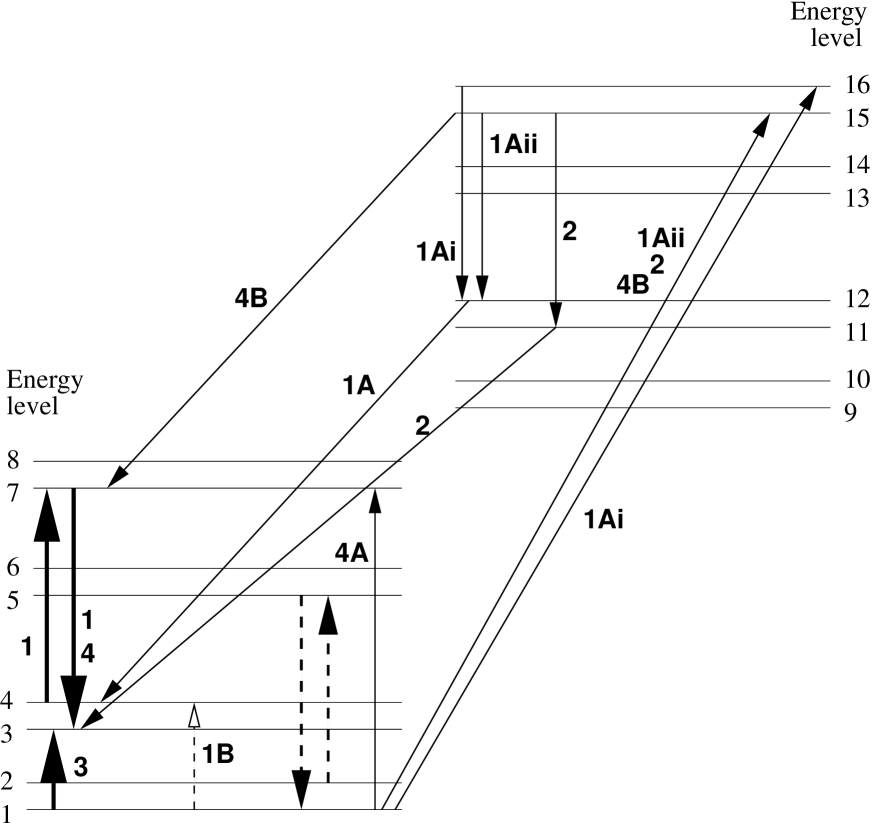
Figure 6: The most important ‘indirect’ pumping routes for the $1612$ MHz transition for the model with a mass-loss rate of $10^{-5}$ M_⊙ yr^-1 at the time of shell-detachment, and for a slab within the main inverted layer (Zone 2). Forward routes only are shown for clarity. All routes rely on the rapid transfer of population from level $2$ to level $1$ via level $5$ (heavy dashed arrows). Transfer from level $1$ to level $3$ is dominated by four routes. If routes $1$ and $2$, which are approximately equally important, are both allocated a strength of $1.0$, then the relative importance of route $3$ is $0.81$, and route $4$ is worth 0.42. Within route $1$, $1A$ is three times stronger than $1B$, and route $4A$ is $2.3$ times stronger than route $4B$. For more detail about the relative importance of particular routes, see the text of Section 5.4. Note that the intervals between energy levels are not drawn to scale. The $F1$ stack of levels is on the left; the $F2$ stack, on the right. For rotational state designations and far-infrared transition wavelengths, see Figure 5.

5.5 The absorbing layer

The next region we consider is slab number $20$, which is within the absorbing layer. Here, the exact coefficients, the analogues of those in eq.(9), are,

$$\left[\!\!\begin{array}[]{rrr}k_{3,3}^{4}=9.03(-5)&k_{2,3}^{4}=2.83(-5)&k_{1,3}^{4}=3.62(-5)\\ k_{3,2}^{4}=5.26(-5)&k_{2,2}^{4}=1.17(-4)&k_{1,2}^{4}=1.66(-4)\\ k_{1,1}^{4}=3.77(-5)&k_{2,1}^{4}=8.92(-5)&k_{3,1}^{4}=2.63(-3)\end{array}\!\!\right]$$ (16)

and comparison with eq.(9) immediately shows that a major change is a diminution of all the coefficients, indicating a generally less efficient transfer of population.

When the investigation with tracer is begun, we find that both the direct and indirect parts of the pump are now anti-inverting: the expression for the direct pump reduces to $-1.223\times 10^{-6}$ s^-1, compared to $+1.081\times 10^{-6}$ s^-1 for the example in Zone 2; the indirect pump yields $-1.019\times 10^{-6}$ s^-1 in the absorbing layer, instead of $+6.457\times 10^{-7}$ s^-1 in the chosen slab from Zone 2. Overall, we find a similar pattern of routes to that available in the inverted case, but with significant changes. Route $1B$ in Fig. 5 has become generally weaker, but remains an inverting route. A partial explanation for the change to absorption is that route $1A$ has gone from being strongly inverting in Zone 2 to strongly anti-inverting in the absorbing layer. As the rate-coefficients $k_{2,4}$ and $k_{4,2}$ are almost equal (as expected for a collision-dominated transtion with a small energy gap) the main change to the coefficients which appear in eq.(13) must involve the coefficients which link levels $3$ and $4$ to level $7$. On examining these coefficients in detail, the switch to inversion in this case results from the $3\rightarrow 7$ transition becoming relatively optically thinner than the $4\rightarrow 7$ transition, in moving from Zone 2 to the absorbing layer.

The second route that produces strong anti-inversion was briefly introduced in Section 5.3 as route $1C$, noting that it made an anti-inverting contribution, even in Zone 2. In the absorbing layer this route, given by

$$1C_{net}\!=\!\frac{k_{2,10}k_{10,14}k_{14,4}k_{4,7}k_{7,3}}{3k_{14,14}^{15}k_{10,10}^{11}k_{7,7}^{8}k_{4,4}^{5}}-\frac{k_{3,7}k_{7,4}k_{4,14}k_{14,10}k_{10,2}}{5k_{4,4}^{5}k_{7,7}^{8}k_{10,10}^{11}k_{14,14}^{15}}$$ (17)

has values of $3.12\times 10^{-7}$ s^-1 for the first (forward) part, and $6.99\times 10^{-7}$ s^-1 for the second (reverse) part. In Zone 2, the analogous values are $3.70\times 10^{-6}$ s^-1 and $3.84\times 10^{-6}$ s^-1. Part of the change towards increased net absorption is explained by the route between levels $3$ and $4$ via level $7$, which route $1C$ shares with $1A$, but there is also a contribution from the group $k_{2,10}k_{10,14}k_{14,4}/(3k_{10,10}^{11}k_{14,14}^{15})$ and its reciprocal, which has also become more anti-inverting. This is definitely not due to the $53$ $\mu$m transitions, $2\rightarrow 10$ and $10\rightarrow 14$, but results from optical depth changes in the $10\rightarrow 14$ transition at $163$ $\mu$m.

Changes to indirect pumping routes are also responsible for about half the anti-inverting power in the absorbing layer. Route $1A$ in Fig. 6 remains inverting, but with reduced effectiveness, because it includes the link from level $4$ to level $3$ via level $7$. This same link causes route $1B$ to fall into an anti-inverting state. For route $3$ the link from level $2$ to level $1$ via level $5$ plays a similar role to the $4\rightarrow 7\rightarrow 3$ sequence. Both operate at a wavelength of $119$ $\mu$m, and differential changes in the optical depth of the upward and downward parts push the whole scheme towards net absorption. The rest of the picture for the indirect part of the pump is much more complicated: the absorption zone has no equivalents of routes $2$ or $4$ with significant strength, but these have been replaced by a complicated web of anti-inverting routes. Of particular importance is a route from level $2$ to level $10$, and thence to level $3$ via level $1$, in which the group

$$Q5=\frac{k_{2,10}k_{10,1}k_{1,3}}{3k_{1,2}^{4}k_{10,10}^{11}}-\frac{k_{3,1}k_{1,10}k_{10,2}}{5k_{10,10}^{11}k_{1,2}^{4}}$$ (18)

has the value $-1.69\times 10^{-7}$ s^-1.

5.6 the outer emission layer, zone 1

The main qualitative differences between this zone and the inner inverted zone, zone 2, lie in the relative importance of the direct and indirect contributions to the inversion, and in the overall complexity. In zone 1, the indirect pump contributes 60.2 per cent of the inversion. The direct pump is similar to that shown in Fig. 5, but has increased complexity due to additional significant routes. In particular, route $1A$ now provides some $80$% of the inversion generated by route $1$, and there is a weaker companion to route $1B$, which operates via level $15$, rather than $16$, The direct route from level $4$ to level $12$, and its reciprocal, is also significant, whilst, importantly, the anti-inverting route $1C$ has diminished.

In the indirect route, we have a similar concentration towards the route which uses only $119$ $\mu$m radiation: the route from level $2$ to level $3$ via level $5$ (route 3 in Fig. 6) provides $94$% of the indirect inversion.

5.7 zone 2 forty years after detachment

Here, we consider the changes to the pumping scheme which result from $40$ yr of expansion of the shell, counting from ‘detachment’, where significant mass loss ends. We consider a layer at the same absolute depth as in Section 5.3 and 5.4. The first observation is that, at this advanced time, the direct pump $(1+\eta)(k_{2,3}^{4}-k_{3,2}^{4})$ is actually mildly larger, in absolute terms, than at shell detachment. The significant reduction in maser output, visible in Fig. 2, must therefore be due to the loss of effectiveness in the indirect pump. This view is confirmed on examination of the coefficients for the indirect pump, which now has a very small negative value. On a more detailed examination of the pump routes, there is also an obvious reason for the change to the indirect pump: both the strongest pump routes, route $1$ and route $2$ in Fig. 6 are now strongly anti-inverting. By comparison, the changes to routes $3$ and $4$ are small. For route $1$, the value of the group $\epsilon_{up}k_{1,4}^{5}k_{4,3}^{5}-\epsilon_{down}k_{3,4}^{5}k_{4,1}^{5}$ has fallen from $2.53\times 10^{-7}$ s^-1 at shell detechment to the strongly anti-inverting value of $-6.62\times 10^{-7}$ s^-1 forty years later. For route $2$, the value of the expression $\epsilon_{up}k_{1,11}^{12}k_{11,3}^{12}-\epsilon_{down}k_{3,11}^{12}k_{11,1}^{12}$ has fallen, over the same period of time, from $2.53\times 10^{-7}$ s^-1 to $-8.52\times 10^{-7}$ s^-1. Although a route via level $9$ has become inverting, it is not nearly enough to compensate for the collapse of routes $1$ and $2$.

Within route $1$, there are the $A$ and $B$ parts. The $B$-part of the route, which involves the lambda-doublet coefficients $k_{1,4}$ and $k_{4,1}$ still has $61$ per cent of the inverting effect it had at shell detachment. The big changes are in the $1A$ routes: the route $1Ai$, via level $16$ retains only $37$ per cent of its inverting effect, whilst route $1Aii$, via level $15$, has become strongly anti-inverting. We note that all three of the routes that have experienced major decreases in their inverting power require $53$ $\mu$m radiation for the initial stage of the forward (inverting) part of the route.

To test the hypothesis that the initial absorption of $53$ $\mu$m radiation is the process most affected by the time evolution of the envelope, we can look at the changes to the upward and downward parts of each group separately. For route $1B$, we find that the downward part of the route, represented by the group $\epsilon_{down}k_{3,11}k_{11,15}k_{15,1}/(k_{11,11}^{12}k_{15,15}^{16})$ has increased from $3.51\times 10^{-7}$ s^-1 to $6.40\times 10^{-7}$ s^-1, whilst the upward counterpart has fallen to just $7.28\times 10^{-8}$ s^-1. The fall in the upward part of the route therefore has the stronger effect. For route $2$, both the upward and downward parts of the routes reduce with time, but the upward part reduces more: the upward group changes from $1.37\times 10^{-6}$ s^-1 to $1.76\times 10^{-7}$ s^-1, whilst the value of the downward expression changes from $1.13\times 10^{-6}$ s^-1 to $8.00\times 10^{-7}$ s^-1.

Of the three coefficients in the upward group, only $k_{1,15}$ is common to route $1Aii$ and route $2$, and it is also the only one which shows a strong change over the $40$ yr of expansion. This coefficient itself falls from $1.993\times 10^{-5}$ s^-1 at shell detachment to $3.906\times 10^{-6}$ s^-1 at the later time. The value of its downward counterpart, $k_{15,1}$, is not noticeably different from its A-value at the later time, indicating that this transition has a negligible collisional component, and that it has become optically very thin. Therefore, although other transitions have significant effects, the largest contribution to the decay of maser radiation is the decreasing mean intensity in the radiation field at $53$ $\mu$m.

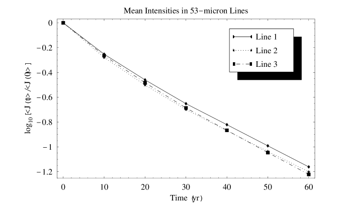
Figure 7: Decay of the angle-averaged intensity, at line centre, of the three important pumping lines at $53$ $\mu$m. These lines are, line $1$ (levels 1-16 in Fig. 6; line $2$ (levels 2-16 in Fig. 5; line $3$ (levels 1-15 in Fig. 6). Absolute values of $<J(0)>$ are, respectively, $2.601\times 10^{-12}$, $1.446\times 10^{-12}$ and $2.598\times 10^{-12}$ W m^-2 Hz^-1. The time origin is at shell detachment.

To test the hypothesis that a lack of $53$ $\mu$m radiation is responsible for the loss of the $1612$ MHz pump, we plot in Fig. 7 the mean (that is angle, but not frequency, averaged) intensities, at line centre, of the three $53$ $\mu$m lines which play important roles in Fig. 5 and Fig.6. These plots are for the same mass-loss rate ($10^{-5}$ M_⊙ yr^-1) as used for the tracer analysis, and for the same depth in zone 2 ($1.289\times 10^{14}$ cm). The mean intensity has been chosen as the function to plot because it is the variable on which the radiative part of the pump directly depends via its products with the Einstein B-coefficients. The three chosen lines are line $1$ ($53.2532$ $\mu$m; levels 1-16 in Fig. 6), line $2$ ($53.2537$ $\mu$m; levels 2-16 in Fig. 5) and line $3$ ($53.2539$ $\mu$m; levels 1-15 in Fig. 6). In the radiation transfer code, lines $2$ and $3$ form an overlapping pair, and all three lines were found in absorption. Lines $1$ and $3$ are believed responsible for the collapse of the strongest part of the pumping scheme in Fig.6. From Fig. 7, we observe that the mean intensity in all three lines, relative to the value at shell detachment, follows a very similar quasi-exponential decay. This tends to confirm that falling energy density in these lines is responsible for the decay of the ‘indirect’ part of the $1612$ MHz pump.

6 Discussion

We have shown that a model comprising a hydrodynamic and photochemical model of the shell of an OH/IR star, and a radiative transfer code for the continuum and OH lines, can reproduce the decay of $1612$ MHz maser emission observed in OH/IR stars. The most pertinent results from the model come from mass loss rates between $1.0\times 10^{-6}$ M_⊙ yr^-1 and $2.0\times 10^{-5}$ M_⊙ yr^-1, where the decay time of the masers varies almost linearly with the mass-loss rate. Decay half-lives derived from unsaturated inversions are comparable with, but slightly larger than, those found observationally. However, if saturation is taken into account, some time would be taken up reducing the degree of saturation, with little change in maser intensity, and thus compressing the observable decay into somewhat shorter intervals than those found with the present model.

The inversions that provide the maser emission are supported in a series of layers within the circumstellar envelope. There are four basic zones: a physically, and optically, thin outer emitting layer which provides only a small amount of the maser gain; an absorbing zone which is sandwiched between the outer emitting zone and a deeper inverted layer, and finally a deep absorbing layer which runs inwards to the edge of the modelled part of the shell. As the shell evolves, following detachment, the zones all tend to move deeper into the shell, and away from the surface (the closest point to the observer). Detailed tracing of the population flow through the OH energy levels has been carried out for representative points in the two inverted layers, and the intervening absorbing layer, with the aim of determining what processes are ultimately responsible for the maser decline.

We find that the strongest pumping routes use FIR transitions at $53$ $\mu$m to cross from the $F1,J=3/2$ ground state to $F2,J=3/2$. This is followed by decay to $F2,J=1/2$, before a ‘cross-stack’ return to the ground state. This type of pump is essentially a modification of the scheme proposed by Elitzur, Goldreich & Scoville [1976] (EGS): the initial stage of the pump relies on $53$ $\mu$m radiation, rather than the $35$ $\mu$m transition used in EGS. However, the variant with a $53$ $\mu$m initial stage is suggested in Elitzur [1981] as an alternative which is likely to operate in cooler envelopes [1987]. We note that in the model used in the present work, the dust temperature in Zone 2 is typically $25$-$40$ K, rather than the $100$-$200$ K needed to drive the $35$ $\mu$m version. Routes that use $35$ $\mu$m radiation are traced in our model, but were never found to be strong enough to include in the discussion. In this connection, the $35$ $\mu$m line was a target in several observations with the ISO satellite. Apart from the Galactic Centre, $35$ $\mu$m lines were detected in absorption by Neufeld et al. [1999] towards VY CMa, and by Sylvester et al. [1997] towards IRC+10420, providing strong support for the EGS model. However, neither of these objects are typical of the moderate to low-mass OH/IR stars considered by the present work. Sylvester et al. also searched for the $53$ $\mu$m lines, but there were no detections either in emission or absorption. $53$ $\mu$m radiation could, however, contribute pumping at a level up to 50% of the $35$ $\mu$m route in IRC+10420 [1997]. Szczerba, He & Chen [2003] looked at 81 OH/IR sources from the ISO archive, all with data covering the OH $35$ $\mu$m transitions. No additional detections were found. A possible interpretation is that most objects in the ISO archive have envelopes which utilize the alternative EGS scheme that is based on $53$ micron radiation.

Spatially, the effects which divide the envelope into the various zones of emission and absorption appear to be controlled, in general terms, by differential optical depth effects in both $53$ $\mu$m and $119$ $\mu$m lines. Moving towards the surface of the envelope, the transition from Zone 2 to the absorbing layer appears to be controlled mainly by changes in the optical depth of $119$ $\mu$m transitions, since pumping routes powered by $53$ $\mu$m radiation remain important, and tend less readily to anti-inversion than those routes which use $119$ $\mu$m transitions only. The boundary between the absorbing layer and Zone 1 appears to be due mainly to a reduction in the strength of the $53$ $\mu$m pumping routes. However, an additional change in the optical depths of $119$ $\mu$m lines must also take place, so that these now drive inversions in Zone 1, which is not so in the absorbing layer.

When the masers decline, we observe that the pumping routes which are lost, that is, which become anti-inverting or significantly less inverting over $40$ yr, are those which require a $53$ $\mu$m upward transition. Population transfer in these routes is dominated by interactions with far infrared radiation. By contrast routes involving transitions within lambda doublets, which are collisionally dominated, maintain their inverting strength quite well over forty years of expansion. We therefore conclude that it is the changes in the radiation field, rather than the kinetic temperature and density in the envelope, which are mainly responsible for the observed fall in maser gain at $1612$ MHz.

Several pumping routes which depend upon FIR radiation still operate well in the envelope $40$ yr after shell detachment. Those which become anti-inverting seem to require the additional feature of an initial upward transition driven by radiation at a wavelength of $53$ $\mu$m, which is the most energetic radiation that is important for the traced pumping schemes. The fact that the loss of the most energetic radiation is important suggests that the underlying change in the envelope, which is responsible for the decay in maser gain, is a cooling of the dust-generated radiation field. This has been confirmed by plotting directly the mean intensity in three $53$ $\mu$m lines as a function of time.

ACKNOWLEDGMENTS

MDG acknowledges PPARC for financial support under the UMIST astrophysics 2002-2006 rolling grant, number PPA/G/O/2001/00483. This research is supported by the National Astronomy and Ionosphere Center, which is operated by Cornell University under a cooperative management agreement with the National Science Foundation. The authors would also like to thank Katherine Lynas for tracing some of the pumping routes, which appear in Figures 5 and 6.

References

- [1981] Booth R.S., Norris R.P., Porter N.D., Kus A.J., 1981, Nature, 290, 382
- [1977] Destombes J.L., Marlière C., Baudry A., Brillet J., 1977, A&A, 60, 55
- [1987] Dickinson D.F., 1987, ApJ, 313, 408
- [1985] Draine B.T., 1985, ApJS, 57, 587
- [1984] Draine B.T., Lee H.M., 1984, ApJ, 285, 89
- [1981] Elitzur M., 1981, in ‘Physical Processes in Red Giants’ (I. Iben & A. Renzini, eds.), Reidel, Dordrecht, p363
- [1976] Elitzur M., Goldreich P., Scoville N., 1976, ApJ, 205, 384
- [1971] Gear C.W., ‘Numerical Initial Value Problems in Ordinary Differential Equations’, Englewood Cliffs, NJ, USA: Prentice Hall
- [1986] Glassgold A.E., Lucas R., Omont A., 1986, A&A, 157, 35
- [2001] Gray M.D., 2001, MNRAS, 324, 57
- [1995] Gray M. D., Field D., 1995, A&A, 298, 243
- [1994] Howe D.A., Rawlings J.M.C., 1994, MNRAS, 271, 1017
- [1982] Huggins P.J., Glassgold A.E., 1982, ApJ, 252, 201
- [1994] Jones K.N., Field D., Gray M.D., Walker R.N.F., 1994, A&A, 288, 581
- [1993] Laor A., Draine B.T., 1993, ApJ, 402, 441
- [2000] Lewis B.M., 2000, ApJ, 533, 959
- [2001] Lewis B.M., 2001, ApJ, 560, 400
- [2002] Lewis B.M., 2002, ApJ, 576, 445
- [2001] Lewis B.M. , Oppenheimer B.D., Daubar I.J., 2001, ApJ, 548, L77
- [2004] Lewis B.M., Kopon D.A., Terzian Y., 2004, AJ, 127, 501
- [1989] Massa D., Savage B., 1989, in proceedings of IAU Symp. 135, ’Interstellar Dust’ (Allamandola L.J., Tielens A.G.G.M. eds.), Kluwer, Dordrecht, p3
- [1977] Mathis J.S., Rumpl W., Nordsieck K.H., 1977, ApJ, 215, 425
- [1983] Morris M., Jura M., 1983, ApJ, 264, 546
- [1987] Netzer N., Knapp G.R., 1987, ApJ, 323, 734
- [1999] Neufeld A.A., Feuchtgruber H., Harwit M., Melnick G.J., 1999, ApJ, 517, L147
- [1994] Offer A.R., van Hemmert M.C., van Dishoeck E.F., 1994, J. Chem. Phys., 100, 362
- [1996] Press W.H., Teukolsky S.A., Vetterling W.T., Flannery B.P., 1996, Numerical Recipes in FORTRAN77: The Art of Scientific Computing (Vol 1), CUP, 2nd edition
- [1995] Randell J., Field D., Jones K.N., Yates J.A., Gray M.D., 1995, A&A, 300, 659
- [1977] Reid M.J., Muhleman D.O., Moran J.M., Johnston K.J., Schwartz P.R., 1977, ApJ, 214, 60
- [2002] Richards A.M.S., 2002, in Migenes V., Reid M.J., eds, Proc. IAU Symposium No. 206, ‘Cosmic Masers: from Protostars to Black Holes’, Mangaratiba, Rio de Janeiro, Brazil, 5th-10th March 2001, p306
- [1985] Scharmer G.B., Carlsson M., 1985, J. Comp. Phys. 59, 56
- [1992] Spaans M., van Langevelde H.J., 1992, MNRAS, 258, 159
- [1978] Spitzer L., 1978, Physical Processes in the Interstellar Medium, Wiley, New York
- [1997] Sylvester R.J. et al., 1997, MNRAS, 291, L42
- [2003] Szczerba R., He H.-H., Chen P.-S., 2003, in ‘Exploiting the ISO Data Archive - Infrared Astronomy in the Internet Age’, (eds. C. Gry et al. ESA SP-511), Siguenza, Spain, 24-27 June 2002, (in the press)
- [1998] Thai-Q-Tung, Dinh-V-Trung, Nguyen-Q-Rieu, Bujarrabal V., Le Bertre T., Gérard E., 1998, A&A, 331, 317
- [1984] van Dishoeck E., Dalgarno A., 1984 ApJ, 277, 576
- [1992] Wood P.R. & Vassiliadis E., 1992, ‘Highlights of Astronomy’, 9, 617 (ed. J. Bergeron)
- [1981] Wood P.R., Zarro D.M., 1981, ApJ, 247, 247
- [1998] Yates J.A., Sylvester R., 1998, proceedings of IAU Symposium 191, Montpellier, France, Aug. 28 - Sept. 1, 1998, poster P4-19