High-energy neutrino emission from X-ray binaries

Abstract

We show that high-energy neutrinos can be efficiently produced in X-ray binaries with relativistic jets and high-mass primary stars. We consider a system where the star presents a dense equatorial wind and the jet has a small content of relativistic protons. In this scenario, neutrinos and correlated gamma-rays result from $pp$ interactions and the subsequent pion decays. As a particular example we consider the microquasar LS I $+61\;303$. Above 1 TeV, we obtain a mean-orbital $\nu_{\mu}$-luminosity of $\sim 5\;10^{34}$ erg/s which can be related to an event rate of 4-5 muon-type neutrinos per kilometer-squared per year after considering the signal attenuation due to maximal neutrino oscillations. The maximal neutrino energies here considered will range between 20 and 85 TeV along the orbit. The local infrared photon-field is responsible for opacity effects on the associated gamma radiation at high energies, but below 50 GeV the source could be detected by MAGIC telescope. GLAST observations at $E_{\gamma}>100$ MeV should also reveal a strong source.

PACS: 95.85.Ry; 98.70.Sa; 13.85.Tp 13.85-t

To Appear in Phys. Rev. D (April 2006 issue).

1 Introduction

The study of high-energy neutrinos from galactic sources is expected to provide important clues for the understanding of the origin of cosmic rays in our Galaxy. Astrophysical sources of high-energy neutrinos should have relativistic hadrons and suitable targets for them, such as radiation and/or matter fields. Rotating magnetized neutron stars are well-known particle accelerators. When they make part of a binary system, relativistic particles may find convenient targets in the companion star and high-energy interactions can take place. It is then natural to consider accreting neutron stars or, more generally, X-ray binaries, as potential neutrino sources (see Bednarek et al. 2005 and references therein[1]).

Neutron stars with high magnetic fields can disrupt the accreting flow, which is channeled through the field lines to the magnetic poles of the system. The magnetosphere of such systems presents electrostatic gaps where protons can be accelerated up to very high energies. Actually, even in the absence of relativistic jets, it is possible to attain hundreds of TeVs (Cheng & Ruderman 1989, 1991 [2, 3]). The accelerated protons, which move along the closed field lines, can impact on the accreting material producing gamma-rays (Cheng et al. 1992a [4], Romero et al. 2001 [5], Orellana & Romero 2005 [6]) and neutrinos (Cheng et al. 1992b [7], Anchordoqui et al. 2003 [8]).

If the magnetic field of the neutron star is not very high, then accretion/ejection phenomena can appear, and the X-ray binary can display relativistic jets, as in the well-known cases of Sco X-1 (Fender et al. 2004 [9]) and LS I $+61\;303$ (Massi et al. 2001, 2004 [10, 11]). The X-ray binary is then called a ’microquasar’. In this case, a fraction of the jet hadrons can reach much higher energies, up to a hundred of PeVs or more, depending on the parameters of the system (see below).

Microquasars can be powered either by a weakly magnetized neutron star or by a black hole (as, for instance, Cygnus X-1). Some of them are suspected to be gamma-ray sources (Paredes et al. 2000 [12], Kaufman-Bernadó et al. 2002 [13], Bosch-Ramon et al. 2005a [14]). Recently, Aharonian et al. (2005) [15] have detected very high-energy emission from the microquasar LS 5039 using the High Energy Stereoscopic System (HESS). In microquasars, the presence of relativistic hadrons in the jets can lead to neutrino production through photo-hadron (Levinson & Waxman 2001 [16], Distefano et al. 2002 [17]) or proton-proton (Romero et al. 2003 [18], Romero & Orellana 2005 [19], Torres et al. 2005 [20], Bednarek 2005 [21]) interactions. In the latter case, the target protons are provided by the stellar wind of the companion.

In the case studied by Romero et al. (2003) [18], which was the base of subsequent models, the wind is assumed to be spherically symmetric. This, however, is not always the case. In particular, microquasars with Be stellar companions present slow and dense equatorial winds that form a circumstellar disk around the primary star and the compact object moves inside. In the present paper we will study how the interaction of the jet with this material can lead to a prominent neutrino source. We shall focus on a specific object, LS I $+61\;303$, for which all basic parameters are rather well-determined in order to make quantitative predictions that can be tested with the new generation of neutrino telescopes (IceCube, in this case [22]). Our results, however, will have general interest for any microquasar with non-spherically symmetric winds. We shall start with a brief description of LS I $+61\;303$.

2 The microquasar LS I $+61\;303$

LS I $+61\;303$ is a Be/X-ray binary system that presents unusually strong and variable radio emission (Gregory & Taylor 1978 [23]). The X-ray emission is weaker than in other objects of the same class (e.g. Greiner & Rau 2001 [24]) and shows a modulation with the radio period (Paredes et al. 1997 [25]). The most recent determination of the orbital parameters (Casares et al. 2005 [26]) indicates that the eccentricity of the system is $0.72\pm 0.15$ and that the orbital inclination is $\sim 30^{\circ}\pm 20^{\circ}$. The best determination of the orbital period ($P=26.4960\pm 0.0028$) comes from radio data (Gregory 2002 [28]). The primary star is a B0 V with a dense equatorial wind. Its distance is $\sim 2$ kpc. The X-ray/radio outbursts are triggered 2.5-4 days after the periastron passage of the compact object, usually thought to be a neutron star. These outbursts can last until well beyond the apastron passage.

Recently, Massi et al. (2001) [10] have detected the existence of relativistic radio jets in LS I $+61\,303$. These jets seem to extend up to about 400 AU from the compact object (Massi et al. 2004 [29]).

LS I $+61\,303$ has long been associated with a gamma-ray source. First with the COS-B source CG135+01, and later on with 3EG J0241+6103 (Gregory & Taylor 1978 [23], Kniffen et al 1997 [30]). The gamma-ray emission is clearly variable (Tavani et al. 1998 [31]) and has been recently shown that the peak of the gamma-ray lightcurve is consistent with the periastron passage (Massi 2004 [11]), contrary to what happens with the radio/X-ray emission, which peaks after the passage. A complete an updated summary of the source is given by Massi 2005 [32].

The matter content of microquasar jets is unknown, although in the case of SS 433 iron X-ray line observations have proved the presence of ions in the jets (Kotani et al. 1994, 1996 [33, 34]; Migliari et al. 2002 [35]). In the present paper we will assume that relativistic protons are part of the content of the observed jets in LS I $+61\,303$. In the next section we will describe the basic features of the model (see Romero et al. 2005 [36] for a detailed discussion of the gamma-ray emission), and then we will present the calculations and results.

3 Model

The system under consideration consists of two objects. The primary is a B-type star that generates a radially outflowing wind. The other is a compact object (CO hereafter, probably a neutron star) moving around in a Keplerian orbit. Their relative position is given by $r(\psi)=a(1-e^{2})/(1-e\cos(\psi))$, where $\psi$ is the orbital phase, $a$ is the semi-major axis of the ellipse and $e$ its eccentricity . The primary presents a nearly equatorial circumstellar disk with a half-opening angle $\phi=15^{\circ}$. Its density is given by $\rho_{\rm w}(r)=\rho_{0}({r}/{R_{*}})^{-n}$ and the wind velocity reads $v_{\rm w}=v_{0}(r/R_{*})^{n-2}$ by continuity. We will adopt $n=3.2$ following Martí and Paredes 1995 [37] (see also Gregory & Neish, 2002 [38]). The wind accretion rate onto the compact object is given by

$$\dot{M}_{\rm c}=\frac{4\pi(G\,M_{\rm c})^{2}\rho_{w}(r)}{v_{\rm rel}^{3}},$$ (1)

where $M_{\rm c}$ is the CO mass and $v_{\rm rel}$ is its velocity relative to the circumstellar wind. The kinetic jet power $Q_{\rm j}$ is coupled to $\dot{M}_{\rm c}$ by $Q_{\rm j}=q_{\rm j}\dot{M}_{\rm c}c^{2}$ (Falcke & Biermann 1995 [39]). In the jet-disk symbiosis model $q_{\rm j}\sim 0.1$ for microquasars in the low-hard state (Fender 2001 [40]). Only a small fraction of the jet particles are highly relativistic hadrons ($\sim 10^{-2}$), and these are confined by the pressure of the cold particles expanding laterally at the local sound speed (see Bosch-Ramon et al. 2005b [41] for a detailed discussion). In the present approach, most of the jet power will consist of cold protons ejected with a macroscopic Lorentz factor $\Gamma\sim 1.25$ (Massi et al. 2001 [10]).

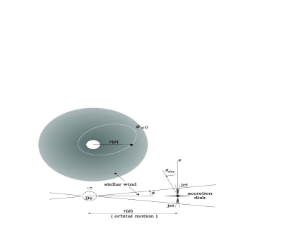
Figure 1: A sketch of the binary system with its elements in detail.

The jet will be a cone with a radius $R_{\rm j}(z)=z(R_{0}/z_{0})$, where $z_{0}=10^{7}$ cm is the injection point and $R_{0}=z_{0}/10$ is the initial radius of the jet (see Romero et al. 2003 [18] and Bosch-Ramon et al. 2005a [14] for additional details). The jet axis, $z$, will be taken normal to the orbital plane. In Figure 1 we show a sketch of the general situation.

We will use a power-law relativistic proton spectrum $N^{\prime}_{p}(E^{\prime}_{p})=K_{p}\;{E^{\prime}}_{p}^{-\alpha}$ (the prime refers to the jet frame). The corresponding relativistic proton flux is $J^{\prime}_{p}(E^{\prime}_{p})=(c/4\pi)N^{\prime}_{p}(E^{\prime}_{p})$ evolving with $z$ as $J^{\prime}_{p}(E^{\prime}_{p})=\frac{cK_{0}}{4\pi}\left(z_{0}/z\right)^{2}{E^{\prime}_{p}}^{-\alpha},$ (conservation of the number of particles is assumed, see Ghisellini et al. 1985 [42]). Using relativistic invariants, it can be shown that the proton flux in the lab (observer) frame becomes (e.g. Purmohammad & Samimi 2001 [43])

$$J_{p}(E_{p},\theta)=\frac{cK_{0}}{4\pi}\left(\frac{z_{0}}{z}\right)^{2}\frac{\Gamma^{-\alpha+1}\left(E_{p}-\beta_{\rm b}\sqrt{E_{p}^{2}-m_{p}^{2}c^{4}}\cos\theta\right)^{-\alpha}}{\left[\sin^{2}\theta+\Gamma^{2}\left(\cos\theta-\frac{\beta_{\rm b}E_{p}}{\sqrt{E_{p}^{2}-m_{p}^{2}c^{4}}}\right)^{2}\right]^{1/2}}.$$ (2)

The angle subtended by the proton velocity direction and the jet axis will be roughly the same as that of the emerging photon ($\theta\approx\theta_{\rm obs}$). $\beta_{\rm b}$ is the bulk velocity in units of $c$, and $\alpha=2.2$ characterizes the power law spectrum (see the list of parameters in Table 1). We adopt a value of 2.2 for the proton power-law index instead of the canonical one of 2.0 given by first order diffusive shock acceleration. This is in order to match the GeV gamma-ray spectrum observed by EGRET [44]. Deviation from the canonical value are likely due to nonlinear effects (see, e.g., Malkov & Drury 2001 [45]). The normalization constant $K_{0}$ and the number density ${n_{0}}^{\prime}$ of particles flowing in the jet at $R_{0}$ can be determined as in Romero et al. (2003) [18].

As long as the particle gyro-radius is smaller than the radius of the jet, the matter from the wind can penetrate the jet diffusing into it. However, some effects, like shock formation on the boundary layers, could prevent some particles from entering into the jet. Actually, the problem of matter exchange through the boundary layers of a relativistic jet is a difficult one. Contrary to cases studied in the literature, where the external medium has no velocity towards the jet (e.g. Ostrowski 1998 [46]), here the wind impacts on the jet side with a velocity that can reach significant values (hundreds of km s^-1). A detailed study of the penetration of the wind into the relativistic flow is beyond the scope of the present paper, so we will treat the problem in a phenomenological way. This can be done by means of a “penetration factor” $f_{\rm p}$ that takes into account particle rejection from the boundary. We will adopt $f_{\rm p}\sim 0.1$, in order to reproduce the observed gamma-ray flux at GeV energies, where opacity effects due to pair creation are unimportant.

We will make all calculations in the lab frame, where the cross sections for proton interactions have suitable parameterizations. Neutral pion decay after high energy proton collisions is a natural channel for high energy gamma-ray production. The differential gamma-ray emissivity from $\pi^{0}$-decays can be expressed as (e.g. Aharonian & Atoyan 1996 [47]):

$$q_{\gamma}(E_{\gamma},\theta)=4\pi\,\eta_{\rm A}\sigma_{pp}(E_{p})\frac{2Z^{(\alpha)}_{p\rightarrow\pi^{0}}}{\alpha}\;J_{p}(E_{\gamma},\theta),$$ (3)

(in ph s^-1 sr^-1 erg^-1), where $Z^{(\alpha)}_{p\rightarrow\pi^{0}}$ is the so-called spectrum-weighted moment of the inclusive cross-section and it is related to the fraction of kinetic proton energy transferred to the pions (see Gaisser 1990 [52]). The parameter $\eta_{\rm A}$ takes into account the contribution from different nuclei in the wind. For standard composition of cosmic rays and interstellar medium $\eta_{\rm A}\sim 1.4$. The proton flux distribution $J_{p}(E_{\gamma})$ (see eq.(2)) is evaluated at $E=E_{\gamma}$, and $\sigma_{pp}(E_{p})\approx 30\times[0.95+0.06\log\;(E_{p}/{\rm GeV})]\;\;(\rm mb)$ [47] is the cross section for inelastic $pp$ interactions at energy $E_{p}\approx 6\xi_{\pi^{0}}E_{\gamma}/K$, for $E_{\gamma}\geq 1$ GeV. Here $K$ is the inelasticity coefficient, and $\xi_{\pi^{0}}$ represents the pion multiplicity. For $\theta$ we will adopt a viewing angle of $\theta_{\rm obs}=30^{\circ}$ in accordance with the average value given by Casares et al. (2005) [26].

The spectral gamma ray intensity (in ph s^-1 erg^-1) is

$$I_{\gamma}(E_{\gamma},\theta)=\int_{V}\ d^{3}\vec{r}\ n(\vec{r})\,q_{\gamma}(E_{\gamma},\theta),$$ (4)

where $V$ is the interaction volume between the jet and the circumstellar disk. The particle density of the wind that penetrates the jet is $n(r)\approx f_{\rm p}\rho_{w}(r)/m_{p}$, and the generated luminosity in a given energy band results

$$L_{\gamma}(E_{\gamma}^{a,b},\theta)=\int_{E_{\gamma a}}^{E_{\gamma b}}\ dE_{\gamma}\ E_{\gamma}\ I_{\gamma}(E_{\gamma},\theta)$$ (5)

Since we are interested in predicting the total gamma ray luminosity measurable on Earth, we must evaluate this integral above a threshold of detection which shall depend on the telescope characteristics. On the other hand, we should keep in mind that $E_{\gamma}$ cannot exceed the maximum gamma ray energy available from the hadronic processes described so far. We will address this issue in more detail in the following section.

4 Hadronic production of neutrinos and gamma rays

In order to discuss the hadronic origin of high energy gamma-rays and neutrinos we have to analyze in more detail pion luminosity and decay. Regarding gamma-rays production, since the branching ratio of charged pions into photons (plus leptons) is about 6 orders of magnitude smaller than that of $\pi^{0}$’s into photons (alone) [27] we shall first concentrate on these neutral parents. Actually, high-energy neutral pions can be produced by relativistic proton collisions in either $pp$ or $p\gamma$ interactions depending on the relative target density of photons and protons in the source region (where the protons are accelerated) and on their relative branching ratios. On the other hand, charged pions will be responsible for high energy neutrinos. In any case, note that both photon and neutrino production at the source are closely related. The $\nu_{\mu}+\bar{\nu}_{\mu}$ differential neutrino flux ($dN_{\nu}/dE_{\nu}$) produced by the decay of charged pions can be actually derived from the differential $\gamma$-ray flux $(dN_{\gamma}/dE_{\gamma})$. Following Alvarez-Muñiz and Halzen (2002) [48], we will find the neutrino intensity and spectral flux by means of an identity related to the conservation of energy (see also Stecker 1979 [49, 50])

$$\int_{E_{\gamma}^{\rm min}}^{E_{\gamma}^{\rm max}}E_{\gamma}{dN_{\gamma}\over dE_{\gamma}}dE_{\gamma}=D\int_{E_{\nu}^{\rm min}}^{E_{\nu}^{\rm max}}E_{\nu}{dN_{\nu}\over dE_{\nu}}dE_{\nu}~{}.$$ (6)

Here ${E_{\gamma}^{\rm min}}$ ($E_{\gamma}^{\rm max}$) is the minimum (maximum) energy of the photons that have a hadronic origin and ${E_{\nu}^{\rm min}}$ and ${E_{\nu}^{\rm max}}$ are the corresponding minimum and maximum energies of the neutrinos. The relationship between both integrals, as given by $D$, depends on the energy distribution among the particles resulting from the inelastic collision. As a consequence, it will depend on whether the $\pi^{0}$’s are of $pp$ or $p\gamma$ origin. Its value can be obtained from routine particle physics calculations and some kinematic assumptions. Let us admit that in $pp$ interactions 1/3 of the proton energy goes into each pion flavor on average. We can further assume that in the (roughly 99.9$\%$) pion decay chains,

$$\pi^{+}\rightarrow\mu^{+}\nu_{\mu}\rightarrow e^{+}\nu_{e}\bar{\nu}_{\mu}\nu_{\mu}\hskip 28.45274pt\pi^{-}\rightarrow\mu^{-}\bar{\nu}_{\mu}\rightarrow e^{-}\bar{\nu}_{e}\nu_{\mu}\bar{\nu}_{\mu}\hskip 28.45274pt\pi^{0}\rightarrow\gamma\gamma,$$

two muon-neutrinos (and two muon-antineutrinos) are produced in the charged channel with energy $E_{\pi}/4$, for every photon with energy $E_{\pi}/2$ in the neutral channel. Therefore the energy in neutrinos matches the energy in photons and $D=1$.

The relevant parameters to relate the neutrino flux to the $\gamma$-ray flux are the maximum and minimum energies of the produced photons and neutrinos, appearing as integration limits in Eq. (6). The maximum neutrino energy is fixed by the maximum energy of the accelerated protons ($E_{p}^{\rm max}$) which can be conservatively obtained from the maximum observed $\gamma$-ray energy $E_{\gamma}^{\rm max}$. Following our previous assumptions

$$E_{p}^{\rm max}=6E_{\gamma}^{\rm max}~{},~{}~{}~{}E_{\nu}^{\rm max}={1\over 2}E_{\gamma}^{\rm max}~{},$$ (7)

for the $pp$ case. The minimum gamma and neutrino energies are fixed by the threshold for pion production. For the $pp$ case

$$E_{p}^{\rm min}=\Gamma~{}{(2m_{p}+m_{\pi})^{2}-2m_{p}^{2}\over 2m_{p}},$$ (8)

where $\Gamma$ is the Lorentz factor of the accelerator relative to the observer. The average minimum neutrino energy is obtained from $E_{p}^{\rm min}$ using the same relations of Eq. (7).

In $p\gamma$ interactions we can assume that neutrinos are predominantly produced via the $\Delta$-resonance. In 1/3 of the interactions a $\pi^{+}$ is produced which decays into two neutrinos of energy $E_{\pi}/4$, and in the other $2/3$ of the interactions a $\pi^{0}$ is produced which decays into two photons of energy $E_{\pi}/2$. Therefore $D=4$. The minimum proton energy is given by the threshold for production of pions, and the maximum neutrino energy is about $5\%$ of the maximum energy to which protons are accelerated, which is much more than that obtained from $pp$ collisions. However, when the production of neutrinos in $p\gamma$ collisions occurs in the acceleration region, the efficiency of conversion into relativistic hadrons is lower than necessary. This is due to the fact that the threshold for electron-positron production is about two orders of magnitude below that for pion production along with the fact that, in this case, the $e^{\pm}$ production cross section is significantly larger. As a result, most of the energy from the acceleration mechanism is transferred to leptons, radiating plenty of photons but no neutrinos.

On the other hand, when purely hadronic collisions are considered, the situation is reverted and pion production becomes the natural production channel. Relativistic protons in the jet will interact with target protons in the wind through the reaction channel $p+p\rightarrow p+p+\xi_{\pi^{0}}\pi^{0}+\xi_{\pi^{\pm}}(\pi^{+}+\pi^{-})$. Then pion decay chains lead to gamma-ray and neutrino emission. Isospin symmetry, which is in agreement with Fermi´s original theory of pion production (where a thermal equilibrium of the resulting pion cloud is assumed) relates the three multiplicities with an equal sign, thus we simply write $\xi_{\pi}$.

We can go a step further and consider energy dependent multiplicities. In this case, the relation between energy maxima is quite different from Eq.(7). According to Ginzburg & Syrovatskii (1964) [51], for inelastic $pp$ interactions we can obtain the gamma ray energy from the proton energy by

$$E_{p}\approx 6\;\xi_{\pi}(E_{p})\ E_{\gamma}/K.$$ (9)

The inelasticity coefficient is $K\sim 0.5$ since on average a leading nucleon and a pion cloud leave the interaction fireball each carrying half of the total incident energy. For the energy dependent pion multiplicity we will follow the prescription adopted by Mannheim and Schlickeiser (1994) [53]

$$\xi_{\pi}\simeq(E_{p}/\rm GeV-1.22)^{1/4}.$$ (10)

Note however that for a proton energy of 1 PeV, the relation between maxima given by eq. (9) would become $E_{p}^{\rm max}\sim 380E_{\gamma}^{\rm max},$ and accordingly $E_{\nu}^{\rm max}\sim{1\over 760}E_{p}^{\rm max}$. This relation implies that the 1 TeV threshold detector IceCube should actually measure some neutrinos provided the microquasar could accelerate protons up to the PeV range. As a matter of fact, Eq. (10) overestimates pion luminosity at energies higher than 10⁴ GeV and the 1/4 root should be relaxed for the proton energies involved in our calculation [53]. Since we have no data about its energy dependence we shall adopt a softer root growing law for $\xi_{\pi}(E_{p})$ which leads to a more reliable relationship between neutrino and proton energies. For the highest proton energies, as given by Eq.(14), one gets $E_{\nu}^{\rm max}\sim{1\over 156}E_{p}^{\rm max}$ at periastron (see Fig.2b). We will promptly see that one can in fact expect for a significant signal to noise relationship in less than one year of operational time of a ‘km³’ telescope.

The point now is whether a microquasar might accelerate protons to such high energies. As mentioned in Bednarek et al. (2005) [1], the maximum energy at which a particle of charge $Z$ can be accelerated, can be derived from the simple argument that the Larmor radius of the particle should be smaller than the size of the acceleration region (Hillas 1984 [56]). If energy losses inside sources are neglected , this maximum energy $E^{M}_{15}$ (in units of $10^{15}$ eV) is related to the strength of the magnetic field $B$ (in units of Gauss) and the size of the accelerating region $R$ (in units of cm) by the following relationship

$$E^{M}_{15}\sim 0.3\;10^{-12}\beta~{}Z~{}B_{G}~{}R_{\rm cm}$$ (11)

where $\beta$ is the velocity of the shock wave or the acceleration mechanism efficiency. Hence, the maximum energy up to which particles can be accelerated depends on the $B\times R$ product. Diffusive particle acceleration through shocks may occur in many candidate sites with sizes ranging from kilometers to megaparsecs. In the case of LS I $+61\;303$, we adopt quasi-parallel shocks, $R\sim R_{\rm j}$ (jet radius), and $B$ given by equipartition with the cold, confining plasma (see Bosch-Ramon et al. 2005b [41]).

For a complete calculation of the magnetic field, we will assume a magneto-hydrodynamic mechanism for the ejection where both matter and field follow adiabatic evolution when moving along the jet. In this conditions it is reasonable to adopt equipartition between the magnetic field energy and the kinetic energy of the jet. This leads directly to the following expression for the magnetic field in the jet reference frame at different distances $z$ from the compact object [57][41]

$$B(z)=\sqrt{8\pi e_{\rm jet}},$$ (12)

where

$$e_{\rm jet}=\frac{\dot{m}_{\rm jet}}{\pi R_{\rm j}^{2}(z)v_{\rm j}m_{p}}E_{\rm k}$$ (13)

is the jet energy density for a cold proton dominated jet. The mean cold proton kinetic energy, $E_{k}$, is taken to be the classical kinetic energy of protons with velocity $v_{\rm j}=c\beta_{\rm b}$. The ejected matter amounts to a fraction of the ratio of accreted matter, namely $\dot{m}_{\rm jet}=q_{\rm j}\dot{M}_{\rm c}$ with $q_{\rm j}\sim 0.1$.

Now, we can proceed and compute the maximum proton energy compatible with this magnetic field by means of the gyro-radius identity

$$E_{p}^{\rm max}=R(z)\ {\rm e}B(z).$$ (14)

This result will be used to compute the maximum jet gamma-ray and neutrino energies which we will need in the next section to calculate both intensities.

In Figure 2 we show the magnetic field (a) and maximum proton energy (b) at the base of the jet in terms of the orbital position for LS I $+61$ 303.

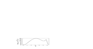
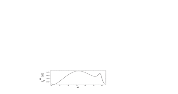
Figure 2: Left (a): Maximal magnetic field in the jet, $B^{\rm max}(\psi)$, as a function of the orbital position of the compact object (in Gauss). Right (b): Highest proton energy compatible with the magnetic field (in PeV) as a function of $\psi$.

As we can see in the figure, the maximum proton energy produced at the base of injection amounts to more than 50 PeV at periastron and lies below 15 PeV near apastron. Note that the minimum does not occur exactly at apastron due to the magnetic field dependence. This is a consequence of the particular orbital variation of the accretion rate. Furthermore, we see that there is a second sharp maximum, readily identified with the function $1/v_{\rm rel}^{3},$ which grows dramatically when the compact object gets far from the primary star and moves more parallel to the weak stellar wind (see also Martí & Paredes 1995 [37] for a discussion of this effect).

5 Flux and event rate of neutrinos

In order to obtain the spectral flux of neutrinos, we need an explicit expression for the neutrino emissivity with the details therein. Instead, we can take eq. (6) so as to extract an expression for $I_{\nu}(E_{\nu})$. Let us write eqs. (6) and (7) as

$$L_{\nu}=D\ L_{\gamma},$$ (15)

and

$$2E_{\nu}=E_{\gamma},$$ (16)

which result from the assumption that, together, one ($\mu$) neutrino and one anti-neutrino carry half one charged-pion energy (note that the number of ($\mu$) neutrinos resulting from $\pi^{+}$ and $\pi^{-}$ decays is equal to the number of gamma rays coming from $\pi^{0}$ since the number of pions produced is the same for the three flavors; same holds for the flux of ($\mu$) anti-neutrinos).

From the last two equations we obtain

$$I_{\nu}(E_{\nu})=4D\ I_{\gamma}(E_{\gamma}=2E_{\nu}).$$ (17)

For $pp$ interactions 1/3 of the proton energy goes to each pion flavor and we have $D=1$. Thus we have for the neutrino intensity

$$I_{\nu}(E_{\nu},\theta)=4\int_{V}dV\ \frac{f_{p}\ \rho_{w}(r)}{m_{p}}\ q_{\gamma}(\vec{r},2E_{\nu},\theta)$$ (18)

Now, we have to compute the convolution of the neutrino flux with the event probability. For signal and noise above 1 TeV we obtain respectively

$$S=T_{\rm obs}A_{\rm eff}\frac{1}{4\pi d^{2}}\ \frac{1}{2\pi}\int_{0}^{2\pi}d\psi\int_{1\rm TeV}^{E_{\nu}^{\rm max}(\psi)}dE_{\nu}\ I_{\nu}(E_{\nu},\psi)\ P_{\nu\rightarrow\mu}(E_{\nu}),$$ (19)

and

$$N=\bigg{[}T_{\rm obs}A_{\rm eff}\Delta\Omega\frac{1}{2\pi}\int_{0}^{2\pi}d\psi\int_{1\rm TeV}^{E_{\nu}^{\rm max}(\psi)}dE_{\nu}\ F_{B}(E_{\nu})\ P_{\nu\rightarrow\mu}(E_{\nu})\bigg{]}^{1/2},$$ (20)

where $T_{\rm obs}$ is the observational time period, $A_{\rm eff}$ is the effective area of the detector, $d$ is the distance to the system, and $\Delta\Omega$ is the solid angle of the search bin. The function

$$F_{B}(E_{\nu})\leq 0.2\ (E_{\nu}/\rm GeV){}^{-3.21}\ \ {\rm GeV^{-1}cm^{-2}s^{-1}sr^{-1}}$$ (21)

represents the $\nu_{\mu}+\bar{\nu}_{\mu}$ atmospheric flux (see Volkova 1980, and Lipari 1993 [58, 59]), and

$$P_{\nu\rightarrow\mu}(E_{\nu})=1.3\ 10^{-6}\ (E_{\nu}/\rm TeV){}^{0.8}$$ (22)

is the probability that a neutrino of energy $E_{\nu}\sim 1-10^{3}$ TeV, on a trajectory through the detector produces a muon (see Gaisser et al. 1995 [60]).

As we have already discussed, the value of the maximal neutrino energy is a function of orbital position of the jet and is given by

$$E_{\nu}^{\rm max}(\psi)\approx\frac{K}{12\xi_{\pi}(\psi)}\ E_{p}^{\rm max}(\psi).$$ (23)

Our estimate for this expression is $E_{\nu}^{\rm max}\approx 85$ TeV at periastron, and about 20 TeV at apastron (see Fig.3).

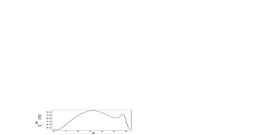
Figure 3: Maximal neutrino energies $E_{\nu}^{\rm max}$ along the orbit (in TeV).

If we now set the features of a km-scale detector such as IceCube [22] in the model ($A_{\rm eff}=1$ km² and $\Delta\Omega\approx 3\ 10^{-4}$sr), and the distance to LS I $+61$ 303 ($d=2$ kpc) we get

$$S/N\mid_{1\rm year}\geq 9.42$$ (24)

for the signal to noise ratio in a one-year period of observation. This is consistent with the upper limit recently reported by Ackermann et al. (2005) from AMANDA-II experiment [61].

Note that the present prediction is restricted to $\mu$-neutrino production at the source. As a matter of fact, there is nowadays strong experimental evidence of the existence of neutrino oscillations which occur if neutrinos are massive and mixed. In 1998 (see Super-Kamiokande [62]) and in 2002 (see K2K [63]) it has been observed, respectively, the disappearance of atmospheric and laboratory muon-neutrinos as expected from flavor oscillations. Also in 2002, the SNO experiment [64] provided solid evidence of solar electron-neutrino oscillations to other flavors. Solar and atmospheric neutrino flux suppression can be explained in the minimal framework of three-neutrino mixing in which the active flavor neutrinos $\nu_{e},\nu_{\mu}$ and $\nu_{\tau}\$ are unitary linear combinations of three mass (Majorana) eigenstates of the neutrino lagrangian [65].

The expected ratios at sources of high-energy neutrino fluxes from $pp$ collisions are $1:2:10^{-5}\$ for the $e,\mu,\tau\$ neutrino flavors, in the range 1 GeV $\leq E_{\nu}\leq 10^{12}$ GeV. The neutrino oscillation effects imply that one should measure different values depending on the distance to the astrophysical source. The estimate is that these ratios become in average $1:1:1\$ for $L(\rm pc)/E(\rm GeV)\geq 10^{-10},\$ where the distance is in parsecs (see Athar et al. 2005 [66]). Also recently, a detailed analysis of supernova remnants reported by Costantini and Vissani (2005) [67] claims a 50$\%$ of muon-neutrino plus muon anti-neutrino flux reduction due to flavor oscillations along astrophysical distances. Note finally, that the neutrino signal measured at Earth might be further attenuated due to matter absorption (see both references above).

6 Luminosity and opacity

As a result of the discussion above, our predictions for both neutrino and gamma ray luminosities between $E_{\nu,~{}\gamma}^{\rm min}=1,2$ TeV and $E_{\nu,~{}\gamma}^{\rm max}$ amount to 5 10³⁴ erg s^-1 for a source such as LS I $+61$ 303.

The total neutrino luminosity is related to the spectral neutrino intensity by means of

$$L_{\nu}=\int_{{E_{\nu}^{\rm min}}}^{E_{\nu}^{\rm max}}dE_{\nu}\ E_{\nu}\ I_{\nu}(E_{\nu})$$ (25)

as we mentioned in Sect. 3. Since we do not have an expression for $I_{\nu}(E_{\nu})$, we can use eq. (6) and relate it to the gamma ray luminosity

$$L_{\gamma}=\int_{{E_{\gamma}^{\rm min}}}^{E_{\gamma}^{\rm max}}dE_{\gamma}\ E_{\gamma}\ I_{\gamma}(E_{\gamma})$$ (26)

which we know in more detail. Now, there is in fact an experimental constraint on this quantity, as recently analyzed by Fegan et al. (2005) [68]. There, it is claimed that, above 0.35 TeV, the total flux of gamma rays that can be produced must satisfy

$$\frac{1}{4\pi d^{2}}\int_{{0.35\rm TeV}}^{\infty}dE_{\gamma}\ I_{\gamma}(E_{\gamma})\leq 1.7\ 10^{-11}{\rm\ ph\ cm^{-2}s^{-1}}.$$ (27)

Our calculations for gamma rays give about four times this value, so we need to show that most of the high-energy gamma rays get absorbed. Of course, the absorption mechanism should not modify the flux of neutrinos. Infrared photon fields can be responsible for TeV photon absorption in the source. To show it, we calculate the optical depth $\tau$ within the circumstellar disk for a photon with energy $E_{\gamma}$

$$\tau(\rho,\,E_{\gamma})=\int_{E_{\rm min}(E_{\gamma})}^{\infty}dE_{\rm ph}\,\int_{\rho}^{\infty}d\rho\ n_{\rm ph}(E_{\rm ph},\rho)\ \sigma_{e^{-}e^{+}}(E_{\rm ph},E_{\gamma}),$$ (28)

where $E_{\rm ph}$ is the energy of the ambient photons, $n_{\rm ph}(E_{\rm ph},\rho)$ is their density at a distance $\rho$ from the neutron star, and $\sigma_{e^{-}e^{+}}(E_{\rm ph},E_{\gamma})$ is the photon-photon pair creation cross section given by

$$\sigma_{e^{+}e^{-}}(E_{\rm ph},\;E_{\gamma})=\frac{\pi r_{0}^{2}}{2}(1-\xi^{2})\left[2\xi(\xi^{2}-2)+(3-\xi^{4})\ln\left(\frac{1+\xi}{1-\xi}\right)\right],$$ (29)

where $r_{0}$ is the classical radius of the electron and

$$\xi=\left[1-\frac{(m_{e}c^{2})^{2}}{E_{\rm ph}E_{\gamma}}\right]^{1/2}.$$ (30)

In Eq. (28), $E_{\rm min}=m_{e}^{2}c^{4}/E_{\gamma}$ is the threshold energy for pair creation in the ambient photon field. This field can be considered as formed by two components, one from the Be star and the other from the cold circumstellar disk, $n_{\rm ph}=n_{\rm ph,1}+n_{\rm ph,2}$. Here,

$$n_{\rm ph,1}(E_{\rm ph},\rho)=\left(\frac{\pi B(E_{\rm ph})}{hc\,E_{\rm ph}}\right)\frac{R_{\star}^{2}}{\rho^{2}+r^{2}-2\rho r\sin\theta}\;,$$ (32)

is the black body emission from the star, and

$$n_{\rm ph,2}(E_{\rm ph},\rho)=\left(\frac{\pi B(E_{\rm ph})}{hc\,E_{\rm ph}}\right)\frac{r^{2}}{\rho^{2}}\;,$$ (33)

corresponds to the emission of the circumstellar disk. In both cases we adopt

$$B(E_{\rm ph})=\frac{2E_{\rm ph}^{3}}{(hc)^{2}\,(e^{E_{\rm ph}/kT_{\rm eff}}-1)}$$ (34)

where $T_{\rm eff,1}=22500$ K and $T_{\rm eff,2}=17500$ K (Martí & Paredes 1995 [37]).

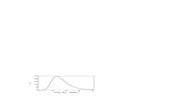
Figure 4: Optical depth at periastron, as a function of $\log(E_{\gamma}/\rm GeV)$.

The mentioned value for $T_{\rm eff,2}$ is valid in the inner region of the disk and thus reliable only near periastron (as one gets far from the central star the temperature of the disk gets lower). Hence we adopt $r=r_{\rm periastr}$. In any case, computing the opacity at periastron, where the luminosity is maximal, will be enough for our purposes of proving that the total gamma-ray luminosity predicted in our model is below the Fegan et al.’s constraint [68]. Figure 4 shows the $E_{\gamma}$ dependence of the optical depth at periastron for an observer at $\theta_{\rm obs}=30^{\circ}$ with respect to the jet axis. The optical depth remains above unity for a wide range of photon energies but a sharp knee takes place at $E_{\gamma}\approx 250$ GeV. For TeV gamma energies it still has an important effect on the luminosity. In particular, the opacity-corrected total flux above $E_{\gamma}=$ 350 GeV drops from 7.16 $10^{-11}$ to 1.42 $10^{-12}$ ph cm^-2 s^-1, lying well below the Fegan et al.’s threshold.

Other observing windows, however, could reveal the presence of a hadronic gamma-ray source at the position of LS I $+61\,303$. In particular, between 1 and 50 GeV the opacity is sufficiently low as to allow a relatively easy detection by instruments like the ground-based MAGIC telescope and the LAT instrument of GLAST satellite. The source is in the Northern Hemisphere, hence out of the reach of HESS telescopes, which recently detected the microquasar LS 5039 . LS I $+61\,303$ is an outstanding candidate to corroborate that high-energy emission is a common property of microquasars. Its location, in addition, makes of it an ideal candidate for IceCube. A neutrino detection from this source would be a major achievement, which would finally solve the old question on whether relativistic protons are part of the matter content of the energetic outflows presented by accreting compact objects.

7 Conclusions

We have analyzed the possible origin of high-energy neutrinos and gamma rays coming from a galactic source. Our specific subject for the analysis has been the microquasar LS I $+61\;303$ because it is a well-studied object of unique characteristics and an appropriate candidate to make a reliable prediction of the neutrino flux from a galactic point source. We performed our calculations within a purely hadronic framework and showed how neutrino observatories like IceCube can establish whether TeV-gamma rays emitted by microquasars are the decay products of neutral pions. Such pions are produced in hadronic jet - wind particle interactions. We improved previous predictions by considering realistic values for the parameters of the system and energy dependent pion multiplicities particularly significant at high energies. Above 1 TeV, we obtained a mean-orbital $\nu$-luminosity of 5 $10^{34}$ erg/s which can be related to an event rate of 4–5 muon-type neutrinos per kilometer-squared per year if we take into account neutrino oscillations. The upper limit of integration depends on the orbital position and is a function of the largest magnetic gyro-radius compatible with the jet dimensions. As a consequence, the maximal neutrino energies here considered range between 20 and 85 TeV along the orbit. Opacity effects on the associated gamma radiation are due to the infrared photon field at the source and result in a significant attenuation of the original $\gamma$-ray signal. Nonetheless, LS I $+61\,303$ might be detectable at low GeV energies with instruments like MAGIC and GLAST. Such a detection, would be crucial to test current ideas of particle acceleration in compact objects.

Acknowledgements

H.R.C. thanks financial support from FUNCAP and CNPq, Brazil. G.E.R. and M.O. are supported by CONICET (PIP 5375) and ANPCyT (PICT 03-13291), Argentina.

Table 1: Basic parameters assumed for the model

Parameter	Symbol	Value
Mass of the compact object	$M_{\rm c}$	1.4 $M_{\odot}$
Jet’s injection point  1	$z_{0}$	50 $R_{\rm g}$
Initial radius	$R_{0}$	$z_{0}/10$
Mass of the companion star	$M_{\star}$	10 $M_{\odot}$
Radius of the companion star	$R_{\star}$	10 $R_{\odot}$
Effective temperature of the star	$T_{\rm eff}$	22500 K
Density of the wind at the base	$\rho_{0}$	$10^{-11}$ gr cm-3
Initial wind velocity2	$v_{0}$	5 km s-1
Jet’s Lorentz factor	$\Gamma$	1.25
Minimum proton energy	${E^{\prime}}_{p}^{\rm min}$	1 GeV
Penetration factor	$f_{\rm p}$	0.1
Orbital axis (cube)	$a^{3}$	$\frac{P^{2}G(M_{\star}+M_{\rm c})}{4\pi^{2}}$
Eccentricity	$e$	0.72
Orbital period	$P$	26.496 d
Relativistic jet power coupling	$q_{j}$	0.01
Index of the jet proton distribution	$\alpha$	2.2
${}^{1}\ \ R_{\rm g}=GM_{\rm c}/c^{2}$.
2 The wind velocity increases from this value up to the escape
velocity according to the velocity law given in the text.

References

- [1] Bednarek, W., Burgio, G. F., Montaruli, T. 2005, New. Astron. Rev., 49, 1
- [2] Cheng K.S., Ruderman M., 1989, ApJ, 337, L77
- [3] Cheng K.S., Ruderman M., 1991, ApJ, 373, 187
- [4] Cheng K.S., et al., 1992a, ApJ, 390, 480
- [5] Romero, G. E.; Kaufman Bernadó, M. M.; Combi, J. A.; Torres, D. F. 2001, A&A, 376, 599
- [6] Orellana, M., & Romero, G.E. 2005, Ap&SS, 297, 167
- [7] Cheng K.S., Cheung T., Lau M.M., & Ng, K.W. 1992b, J. Phys. G, 18, 725
- [8] Anchordoqui L.A., et al., 2003, ApJ, 589, 481
- [9] Fender, R.P., et al. 2004, Nature, 427, 222
- [10] Massi, M., Ribó, M., Paredes, J.M., et al. 2001, A&A, 376, 217
- [11] Massi, M. 2004, A&A, 422, 267
- [12] Paredes, J. M., Martí, J., Ribó, M., & Massi, M. 2000, Science, 288, 2340
- [13] Kaufman Bernadó, M. M., Romero, G. E., & Mirabel, I. F. 2002, A&A, 385, L10
- [14] Bosch-Ramon, V., Romero, G.E., & Paredes, J.M. 2005a, A&A, 429, 267
- [15] Aharonian, F.A., et al. 2005, Science, 309, 746
- [16] Levinson, A., & Waxman, E. 2001, Phys. Rev. Lett., 87, id. 171101
- [17] Distefano, C., Guetta, D., Waxman, E., & Levinson, A. 2002, ApJ, 575, 378
- [18] Romero, G.E., Torres, D.F., Kaufman Bernadó, M.M. & Mirabel, I.F. 2003, A&A, 410, L1
- [19] Romero, G.E. & Orellana, M. 2005, A&A, 439, 237
- [20] Torres, D.F., Romero, G.E., Mirabel, F. 2005, Chin. J. Astron. Astrophys. Suppl., 5, 183
- [21] Bednarek, W., 2005, ApJ, 631, 466
- [22] IceCube 2002, http://icecube.wisc.edu/
- [23] Gregory, P.C, & Taylor, A.R. 1978, Nature, 272, 704
- [24] Greiner, J. & Rau, A. 2001, A&A, 375, 145
- [25] Paredes, J.M., Martí, J., Peracaula, M, & Ribó, M. 1997, A&A, 320, L25
- [26] Casares, J., Ribas, I., Paredes, J.M., et al. 2005, MNRAS, 360, 1105
- [27] S. Eidelman et al., Phys. Lett. B 592, 1 (2004) and 2005 partial update for the 2006 edition. Review of Particle Physics, PDG, http://pdg.lbl.gov/2005/listings/mxxxcomb.html
- [28] Gregory, P.C. 2002, ApJ, 575, 427
- [29] Massi, M., Ribó, M., Paredes, J.M., et al. 2004, A&A, 414, L1
- [30] Kniffen, D.A., Alberts, W.C.K., Berstch, D.L., et al. 1997, ApJ, 486, 126
- [31] Tavani, M., Kniffen, D.A., Mattox, J.R., et al. 1998, ApJ, 497, L89
- [32] Massi, M. 2005, Introduction to Astrophysics of Microquasars, Habilitationsschrift, Bonn
- [33] Kotani, T., Kawai, N., Aoki, T., et al. 1994, PASJ, 46, L147
- [34] Kotani, T., Kawai, N., Matsuoka, M., & Brinkmann, W. 1996, PASJ, 48, 619
- [35] Migliari, S., Fender, R. & Méndez, M. 2002, Science, 297, 1673
- [36] Romero, G.E., Christiansen, H.R., Orellana, M. 2005, ApJ, 632, 1093
- [37] Marti, J., & Paredes, J.M. 1995, A&A, 298, 151
- [38] Gregory, P.C., & Neish, C. 2002, ApJ, 580, 1133
- [39] Falcke, H., & Biermann, P. L. 1995, A&A, 293, 665
- [40] Fender, R.P. 2001, MNRAS, 322, 31
- [41] Bosch-Ramon, V., Romero, G.E., & Paredes, J.M. 2006, A&A, 447, 263
- [42] Ghisellini, G., Maraschi, L., & Treves, A. 1985, A&A, 146, 204
- [43] Purmohammad, D., & Samimi, J. 2001, A&A 371, 61
- [44] Hartman, R.C., Bertsch, D.L., Bloom, S.D., et al. 1999, ApJS, 123, 79
- [45] Malkov, M.A., & Drury, L. O’C. 2001, Rep. Prog. Phys., 64, 429
- [46] Ostrowski, M. 1998, A&A, 335, 134
- [47] Aharonian, F. A., & Atoyan, A. M. 1996, A&A, 309, 917
- [48] Alvarez-Muñiz, J. & Halzen, F. 2002, ApJ, 576, L33
- [49] Stecker, F. W. 1979, ApJ, 228, 919
- [50] Stecker, F. W. & Salamon, M. H. 1996, Space Science Reviews, 75, 341
- [51] Ginzburg, V.L. & Syrovatskii, S.I. 1964, Sov. Astron. 8, 342
- [52] Gaisser, T.K. 1990, Cosmic Rays and Particle Physics, Cambridge University Press, Cambridge
- [53] Mannheim, K. & Schlickeiser, R., 1994, A&A, 286, 983
- [54] Begelman M.C., Bronislaw R., Sikora M., 1990, ApJ 362, 38
- [55] Orth, C.D. and Buffington, A., 1976, ApJ 206, 312
- [56] Hillas, A. M. 1984, ARAA 22, 425
- [57] Blandford, R.D., & Konigl, A. 1979, ApJ, 232, 34
- [58] Volkova, L. V. 1980, Yad. Fiz., 31, 1510, [1980, Sov. J. Nucl. Phys., 31, 784].
- [59] Lipari, P. 1993, Astrop. Phys. 1, 195
- [60] Gaisser, T. K., Halzen, F., & Stanev, T. 1995, Phys. Rep., 258, 173, and references therein, Erratum-ibid. 1995, 271, 355
- [61] Ackermann, M., et al. 2005, Phys. Rev. D, 71, id. 077102
- [62] Super-Kamiokande 1998, Fukuya Y. et al. Phys. Rev. Lett. 81, 1562
- [63] K2K, Ahn, M.H. et al. 2003, Phys. Rev. Lett. 87, id. 071301
- [64] SNO 2002, Ahmad Q. R. et al. Phys. Rev Lett. 89, id. 011301
- [65] Giunti C., Laveder M. 2004, Developments of Quantum Physics, ed. F. Columbus and V. Krasnoholovets, Nova Sci. Pub.
- [66] Athar H., Kim C.S., and Lee J., astro-ph/0505017
- [67] Costantini, M.L. and Vissani, F. 2005, Astrop. Phys. 23, 477
- [68] Fegan, S., et al. 2005, ApJ 624, 638
- [69] Aharonian, F.A., Anchordoqui, L.A., Khangulyan, D., Montaruli, T., astro-ph/0508658