Implications of the Cosmic Background Imager Polarization Data

Abstract

We present new measurements of the power spectra of the E-mode of CMB polarization, the temperature T, the cross-correlation of E and T, and upper limits on the B-mode from 2.5 years of dedicated Cosmic Background Imager (CBI) observations. Both raw maps and optimal signal images in the $uv$-plane and the sky plane show strong detections of the E-mode (11.7$\sigma$ for the EE power spectrum overall) and no detection of the B-mode. The power spectra are used to constrain parameters of the flat tilted adiabatic $\Lambda$CDM models: those determined from EE and TE bandpowers agree with those from TT, a powerful consistency check. There is little tolerance for shifting polarization peaks from the TT-forecast locations, as measured by the angular sound crossing scale $\theta=100/\ell_{s}=1.03\pm 0.02$ from EE and TE cf. $1.044\pm 0.005$ with the TT data included. The scope for extra out-of-phase peaks from subdominant isocurvature modes is also curtailed. The EE and TE measurements of CBI, DASI and BOOMERANG are mutually consistent, and, taken together rather than singly, give enhanced leverage for these tests.

1 Introduction

Polarization of the cosmic microwave background (CMB) at the $\sim 10\%$ level has been forecast for decades e.g., Bond & Efstathiou (1984), but only after a long experimental struggle was it detected and firmly established, from measurements by the DASI (Kovac et al., 2002), WMAP (Kogut et al., 2003), CBI (Readhead et al., 2004b), CAPMAP (Barkats et al., 2005) and Boomerang (Masi et al., 2005; Montroy et al., 2006; Piacentini et al., 2006) experiments. The CBI (Padin et al., 2002; Readhead et al., 2004b) is a 13-element interferometer located at 5080 meters in the Chilean Andes operating in ten 1-GHz bands from 26 GHz to 36 GHz. The CBI has been observing the polarization of the CMB since its inception in late 1999, and since 2002 September has been operating in a polarization optimized configuration with 42 polarization-sensitive baselines. The first CBI polarization limits (Cartwright et al., 2005) used only 12 polarization-sensitive baselines. As part of the polarization optimization, we adopted the achromatic polarizers designed by Kovac and described in Kovac et al. (2002). The first CBI detections in the polarization-optimized configuration included data taken from 2002 September to 2004 May (Readhead et al., 2004b). In this paper, we present and analyze the implications of CBI polarization for our complete 2002 September to 2005 April polarization dataset. This represents a 54% increase in integration time over the results reported earlier (Readhead et al., 2004b).

In § 2, we present an abbreviated description of the data and its analysis that leads to the compression of the data on to maps in $\ell$-space, a natural space for interferometry of the CMB, and further compression on to power spectra. A detailed description of the experiment, our analysis procedure and results of data quality tests will be given in Myers et al. (2006, in preparation). We use our improved EE and TE power spectra to test consistency of cosmological parameters with results forecast from TT, for minimal inflation-motivated tilted $\Lambda$CDM models in § 3.2 and hybrid models with an additional subdominant isocurvature component in § 3.4. Special attention is paid to overall amplitudes and pattern-shifting parameters in § 3.3 and § 3.5.

2 Processing of the CBI Polarization Data

2.1 The Polarization Data and the CBI pipeline

The CBI instrument is described by Padin et al. (2002) and the observing and data reduction procedures used for CMB polarization studies are described in Readhead et al. (2004b). Observations were made of four mosaic fields, labeled $02^{\rm h}$, $08^{\rm h}$, $14^{\rm h}$, and $20^{\rm h}$ by right ascension, each having roughly equal observing time. The $20^{\rm h}$ field was a deep $4.5^{\circ}\times 0.75^{\circ}$ $20^{\rm h}$ strip of $6$ pointings separated by $45^{\prime}$. The fwhm of the CBI primary beam is $45^{\prime}$. The other three mosaics were $6\times 6$ pointings each covering a $4.5^{\circ}\times 4.5^{\circ}$ square. The CBI recorded visibilities on 78 baselines (antenna pairs). We note that the data in Readhead et al. (2004b) used only 12 of the 13 antennas, or 66 baselines, due to a software error, which has now been corrected. This error resulted in a  15% loss in sensitivity, but did not bias results. The data were calibrated by reference to standard sources with an uncertainty of 1.3% in flux density (Readhead et al., 2004b). Six of the antennas were set to receive right circular polarization ($R$) and seven left ($L$), so each visibility measurement represents one of the four polarization products $RR,RL,LR,LL$. The copolar products $RR$ and $LL$ are sensitive to total intensity or brightness temperature T (under the assumption that the circular polarization V is zero, as expected), while $RL$ and $LR$ are sensitive to linear polarization which can be divided into grad-mode E and curl-mode B components. In the small angle approximation, where the celestial sphere can be described by a tangent plane (“image” or “sky” plane), the angular spherical harmonic multipoles defining the CMB radiation field, labeled by ($\ell,m$), become Cartesian components of $\ell$, $(\ell_{u},\ell_{v})$. In this same approximation, interferometer visibilities sample the Fourier transform of the sky brightness, with $(u,v)$ as the conjugate variables to angles on the celestial plane; this “$uv$-space” is related to “$\ell$-space” by $(\ell_{u},\ell_{v})=2\pi$(u,v). Each interferometer baseline is therefore sensitive to emission on angular scales centered on spherical harmonic multipole $\ell=2\pi x$ where $x$ is the antenna separation in wavelengths.

The visibilities are processed by convolution with an $\ell$-space gathering kernel to produce gridded estimators $\Delta_{iQ}$ for polarizations $i=$T,E,B and covariance matrix elements $C_{N(ii^{\prime})QQ^{\prime}}$, $C_{T(ii^{\prime})QQ^{\prime}}$, $C_{P(ii^{\prime})QQ^{\prime}}$ for (Gaussian) instrumental noise, (Gaussian) CMB signals, and projection templates associated with point sources and ground spillover (Myers et al., 2003; Readhead et al., 2004b). This gridding compresses the $\sim 10^{7}$ visibilities to $\sim 10^{4}$ $\ell$-space “pixels” (labeled by $Q$) without loss of essential information.

For calculation of angular power spectra, the gridded estimators and covariance matrices are passed to a maximum likelihood procedure which estimates the CMB polarization bandpowers $q_{Xb}$ in band $b$, $X$=$(ii^{\prime})$=TT,EE,TE,BB, associated noise bandpowers $q_{NXb}$, a Fisher (or likelihood curvature) matrix $F_{Xb,X^{\prime}b^{\prime}}$ whose inverse encodes the variance around the maximum likelihood, and $\ell$-space window functions $W_{Xb\ell}$. The $q_{Xb}$ are defined by the expansion of the spectra ${\cal C}^{X}_{\ell}=\sum_{b}q_{Xb}{\cal C}^{X}_{\ell b}$. (Here ${\cal C}^{X}_{\ell}\equiv\ell(\ell+1)\langle a_{i\ell m}a_{i^{\prime}\ell m}^{*}\rangle/2\pi$, where $a_{i\ell m}$ denotes the multipole coefficients of the signal $s_{i}$, $i=$T,E,B.) To determine bandpowers, we use (theory-blind) flat ${\cal C}^{X}_{\ell b}$ shapes with top hat binning (unity inside and zero outside of the band). The window functions from the pipeline convert theory power spectra ${\cal C}^{X}_{\ell}$ into bandpowers $q_{Xb}=\sum_{\ell}{\cal C}^{X}_{\ell}W_{Xb\ell}\,(\ell+1/2)/(\ell(\ell+1))$ to compare with the observed ones.

2.2 The Power Spectra

Fig. 1 shows the CBI maximum likelihood bandpowers and their inverse-Fisher-matrix errors. The numerical values are given in Table 1. To minimize band-to-band correlations only 7 bands are shown for EE, but we use about twice as many bands for our cosmic parameter analyses. A nonlinear transformation to a Gaussian in the “offset lognormal” combination $\ln(q_{Xb}+q_{NXb})$ is used to give a more accurate representation of the bandpower likelihood surface (Bond et al., 2000; Sievers et al., 2003). Fig. 2 shows the spectra of pairs of fields of the CBI data (which have better sensitivity than individual fields). These demonstrate that the remarkably good agreement between the CBI EE spectrum and the fiducial model for EE evident in Fig. 1 is due to random chance.

Table 1: CBI 7-Band Power Spectra (${\cal C}_{\ell}$ in $\mu\rm{K}^{2})$.

$\ell$-range	TT	EE	TE	BB
$<600$	$2971\pm 260$	$12.5\pm 3.9$	$-16.9\pm 24.4$	$0.8\pm 2.8$
$600-750$	$1925\pm 252$	$38.3\pm 7.6$	$-28.5\pm 31.3$	$-1.9\pm 4.0$
$750-900$	$2475\pm 304$	$3.6\pm 9.9$	$-77.6\pm 41.9$	$3.8\pm 11.0$
$900-1050$	$1126\pm 248$	$47.2\pm 20.6$	$-35.5\pm 53.7$	$-2.6\pm 17.2$
$1050-1200$	$1256\pm 239$	$11.3\pm 17.8$	$-82.8\pm 45.7$	$21.1\pm 16.1$
$1200-1500$	$841\pm 137$	$25.0\pm 15.2$	$-61.7\pm 35.7$	$-9.9\pm 12.0$
$>1500$	$256\pm 118$	$-20.3\pm 35.4$	$42.0\pm 59.6$	$-22.6\pm 31.6$

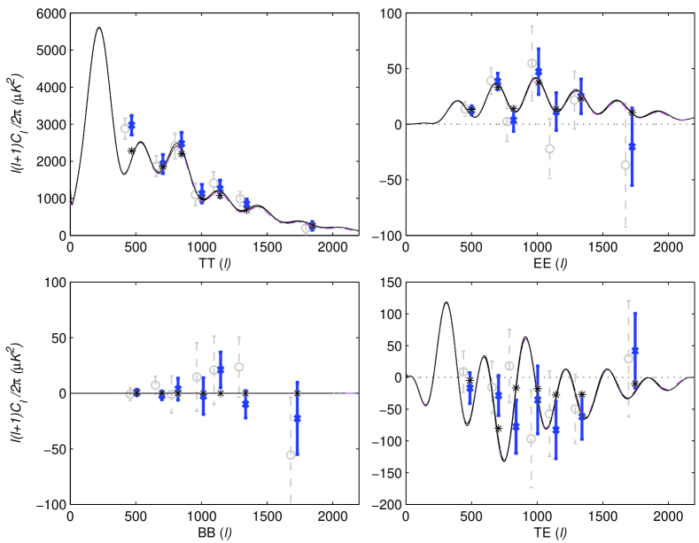
Figure 1: The blue crosses show power spectra ${\cal C}_{\ell}^{X}$ as a function of multipole $\ell$ derived from the CBI 2002 September - 2005 April data, for the total intensity TT, the grad polarization EE, the curl polarization BB, and cross-correlation TE. The magenta dashed curve is a flat power-law $\Lambda$CDM model which best-fits the WMAP, CBI, and ACBAR CMB data (Spergel et al., 2003). It is very nearly the black fiducial ${\cal C}_{\ell}^{X({\rm s})}$ which best-fits WMAP1+CBI+DASI+B03 TT+EE+TE, whose parameters are given in Table 2. The black asterisks show the expected values of the bandpowers calculated from the fiducial model using the window functions. The $\chi^{2}$ values of the data relative to the fiducial model are 13.1, 2.25, 2.90, and 8.43 for TT, EE, BB, and TE for 7 degrees of freedom. As expected, the BB spectrum is consistent with zero, with a single-band amplitude of $0.2\pm 1.6\,\mu\rm{K}^{2}$, and a 95% upper limit of $3.76\,\mu\rm{K}^{2}$. (The grey circles show the results of Readhead et al. (2004b) for comparison. The shrinking in error bars is primarily due to the 54% increase in the data.) The CBI’s low-$\ell$ ($\ell\mathrel{\hbox to0.0pt{\lower 3.0pt\hbox{$\mathchar 536\relax$}\hss}\raise 2.0pt\hbox{$\mathchar 316\relax$}}360$) response is set by the details of the sidelobes of the primary beam, which are difficult to measure; analysis with finer bins shows that the apparent discrepancy in the first TT bin plotted here is confined to $\ell<360$ where the wings of the primary beam are picking up the first Doppler peak. Consequently we neglect the $\ell<360$ TT from CBI in further analysis. The data have been offset in $\ell$ for clarity.

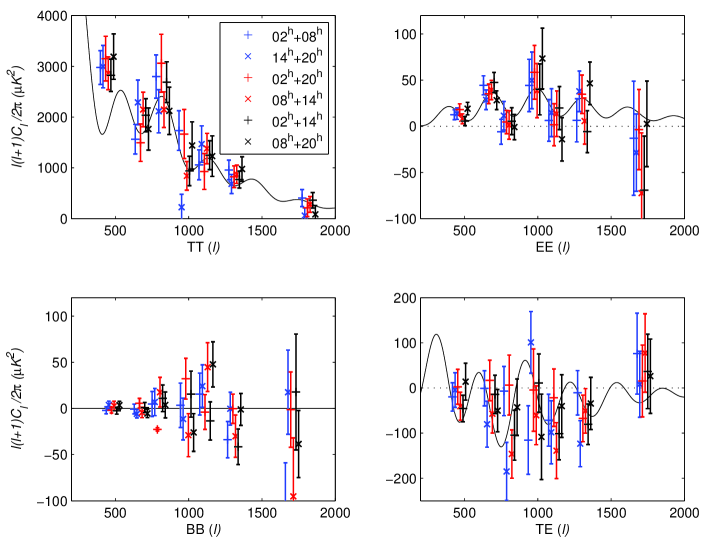
Figure 2: The power spectra for the 6 distinct pairs of CBI fields, each denoted by the colors and symbols indicated in the TT panel. For example. the blue +’s show the $02^{h}+08^{h}$ fields and the blue x’s show the $14^{h}+20^{h}$ fields. The pairs of spectra plotted with the same color are disjoint data sets and hence have meaningful $\chi^{2}$ values. For EE, the $\chi^{2}$ values of the disjoint subsets are 2.98 ($02^{h}+08^{h}$ vs. $14^{h}+20^{h}$), 8.55 ($02^{h}+14^{h}$ vs. $08^{h}+20^{h}$), and 3.67 ($02^{h}+20^{h}$ vs. $08^{h}+14^{h}$) for 7 degrees of freedom. This confirms that the remarkably low $\chi^{2}$ (2.25 for 7 dof) of the joint EE spectrum relative to the fiducial model is due to random chance. The points have been spread in $\ell$ about the bin center for clarity.

If the overall amplitude of $C_{P}$ is set to a large value then the “nuisance” modes represented in the construction of the matrix are projected out. This is essential for ground subtraction and point source projections for T. As discussed in Readhead et al. (2004b), where we project out the brightest $\sim$20% of NVSS sources in E and B, we see no evidence for any polarized point sources in the CBI data. In particular, for CBI the EE spectrum is strongly detected while the BB spectrum is consistent with zero, whereas uncorrelated polarized point sources give rise to (roughly) equal amounts of power in EE and BB. Neither polarization power spectrum rises like $\ell^{2}$ as would be expected from an appreciable point source signal. The spectra with and without the brightest $\sim$20% of NVSS sources projected out in polarization are very similar, with no systematic trend in the differences. Finally, there are no sources visible in the CBI polarization maps. Consequently, in this work, we do not project out any sources in polarization. The nature of the 30 GHz polarized radio source population is currently poorly known, but some models have been devised based on extrapolation from lower frequency surveys. These generally indicate that contamination of the EE and BB power spectra should be negligible for the CBI $\ell$ range, observing frequency, and sensitivity levels, e.g.,  Tucci et al. (2004) Further discussion of this issue will be presented in Myers et al. (2006, in preparation).

2.3 Raw Maps and Signal Reconstructed Maps

The gridded estimators allow us efficiently to reconstruct the polarization of the CMB. We use the fact that E and B are real field components that completely describe the polarization field to present E and B sky images in Figs. 3(a), 5(a). These images are created by Fourier transforming the ground-filtered $\ell$-space estimators $\Delta_{{\rm E}Q}$ and $\Delta_{{\rm B}Q}$. These $\Delta_{{\rm E}Q}$ and $\Delta_{{\rm B}Q}$ in turn are convolved representations of the true $\ell$-space $\tilde{\rm E}$ and $\tilde{\rm B}$ which are related to the linear polarization Stokes parameters Q and U (Kovac et al., 2002). These novel E and B images and $\ell$-space maps differ from the traditional polarization “headless” vector plots based on decomposing the images in Stokes Q and U into E-like and B-like components, as they are direct representations of the E and B fields and their transforms. Note that due to the non-local transformation relating E and B to the Q and U fields on the sky, e.g., Lewis et al. (2002); Bunn et al. (2003), the E and B images do not show polarized “objects” but coherences in the polarization field.

The dominant ground contamination has been removed from the estimators by forming $C_{N}(C_{N}+C_{P})^{-1}\Delta$ in the large $C_{P}$ limit. Here $C_{N}$ serves to regularize $C_{P}$. Other regularizers, such as $C_{N}+C_{T}$, give virtually identical results. The images generated from the estimators include the effects of the observing strategy and of the gridding process, which include the mosaic pattern, $uv$ coverage, the primary beam, and noise-weighting, similar to a standard interferometric “dirty map”. Hence the raw images are not faithful reconstructions of true intensity and polarization. Furthermore, the Fourier transform of the regular mosaic pattern introduces “sidelobes” in the $\ell$-space map made from the raw estimators. Therefore, filtering and deconvolution can be beneficial to our maps.

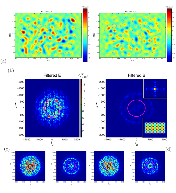
Figure 5: (a) Raw maps of the (approximate) E and B signals from the $02^{h}$ mosaic field for $\ell<1000$. The two northern strips in this field have substantially less data than the four southernmost strips; to keep the noisy northern strips from visually dominating the map, they have not been included in the maps. A filter has been applied to remove the mean-mode (ground) signal, which would otherwise dominate the maps. The variance in the E map is 1.71 times larger than the variance in the B map (which is consistent with the noise). The circles show the fwhm of each of the 24 CBI pointings used in the maps (all 36 mosaic pointings are used in producing the spectrum). (b) The modulus of the optimal (Wiener-filtered) signal maps seen in the gridded $(\ell_{u},\ell_{v})$ plane using our signal reconstruction process, where $(\ell_{u},\ell_{v})=2\pi(u,v))$. The maps have been normalized to $\sqrt{{\rm C}_{\ell}}$, equivalent to plotting $a_{\ell,m}$’s for a full-sky map. The radius of the magenta circles is $\ell=630$, the peak of the CBI’s sensitivity. The striping apparent in the E image is due to the ground filter removing Fourier modes equal to the separation of the mosaic fields in RA. The EE to BB power ratio is 24. The ring at $\ell\sim 1000$ in the B image is due to the $\sim 1.3\sigma$ bandpower value in the fifth BB bin which enters into the filter. The upper inset in the B map is the average mosaic smoothing kernel ${\cal B}$ we chose to smooth the reconstructed maps. The strong anisotropy in $\ell_{u},\ell_{v}$ in Fig. 3 is not there in this square map. The compactness of ${\cal B}$ relative to that of Fig. 3 demonstrates the improved $\ell$-space resolution of a mosaic, at a cost of signal to noise ratio. The cross pattern extending from the central peak of ${\cal B}$ arises from the Fourier transform of the mosaic pattern on the sky. The lower inset is the sky plane representation of $\cal{B}$. (c,d) show two sample realizations of the fluctuations $\delta s=s-\langle s|\Delta\rangle$ on the same scale as (b).

Figs. 3,5(b) show optimal Wiener-filter $\ell$-space maps. These are smoothed mean signals given the observations,

$$\langle s|\Delta\rangle={\cal B}{\rm R}^{\dagger-1}C_{T}C_{tot}^{-1}\Delta\,,\ C_{tot}\equiv C_{N}+C_{P}+C_{T}\,.$$ (1)

Here the matrix ${\rm R}$ takes signal-space into data-space, with $\Delta={\rm R}s+n$, where $s$ is the signal, ${\cal B}$ is a smoothing kernel, and $n$ is the map-noise, including ground and source projection terms. One is free to choose the basis in which to describe the true sky signals $s_{i}$, e.g., as Stokes parameters on the sky relative to a fixed sky-basis or as a set of $a_{i\ell m}$ coefficients or (in the small angle limit) as the set of related Fourier transform coefficients. For the CBI, and interferometers in general, it is natural to express the $s_{i}$ in the $\ell$-basis, as in Figs. 3,5(b), but we also show the sky plane version in Fig. 4. The $C_{T}^{X}=\sum q_{Xb}C_{Tb}^{X}$ used in the signal reconstructions are derived from the data using the measured bandpowers $q_{Xb}$ (set to zero if negative) and the top-hat band matrices $C_{Tb}^{X}$, and hence are “theory-blind”.

Typically the signal-space dimension would be larger than the data-space dimension so ${\rm R}$ would not be invertible. By modeling the $(\ell_{u},\ell_{v})$-plane only at points where we have estimators, the two dimensions are equal, ${\rm R}$ becomes square, and is, in principle, invertible. In practice ${\rm R}$ has an enormous condition number, so we remove poorly measured modes with eigenvalues $<10^{-4}$ of the largest eigenvalue of ${\rm R}$ in constructing the ${\rm R}^{-1}$ operator. This makes the reconstruction better conditioned and the results are insensitive to variations in the eigenvalue cut. The remaining “noise” in ${\rm R}^{-1}$ is controlled by reconvolution with a smooth regularizer ${\cal B}$.

We have freedom in the choice of the smoothing kernel ${\cal B}$. The one we choose for the images is a natural one associated with the map. Letting the pixel be denoted by the vector ${\bf Q}=(\ell_{u},\ell_{v})$, the matrix ${\rm R}$ has components ${\rm R}$_Q,Q+δℓ, where the vector $\delta\ell$ goes over the region of $\ell$-space that contributes to the pixel in question. ${\rm R}$ tends to be only roughly independent of ${\bf Q}$. We take our smoothing kernel ${\cal B}$_δℓ to be the average of ${\rm R}$_Q,Q+δℓ, over all pixels ${\bf Q}$. As can be seen in the insets in Figs. 3,5(b), this is very nearly the Fourier transform of the mosaic pattern on the sky, as is required to make the sky plane images reflect the area actually observed. For the strip ${\cal B}$_δℓ is quite asymmetric, as shown in Fig 3. For the other three square CBI polarization fields, the ${\cal B}$_δℓ is nearly symmetric, as shown in Fig 5. There are low-level ”sidelobes” in the $\ell_{u}$ and $\ell_{v}$ directions due to the mosaic spacing of $45^{\prime}$. Figure 4 shows the sky plane (as opposed to $\ell$-space) representation of the reconstructed signal maps for the deep strip. The agreement between the raw E image in Fig. 3(a) and the reconstructed E image in Fig. 4 is quite good.

To assess how well the mean field $\langle s|\Delta\rangle$ describes the actual distribution of signal on the sky, it is important to see how large the fluctuations $\delta s\equiv s-\langle s|\Delta\rangle$ are about it. For Gaussian signals the statistics of the (smoothed) $\delta s$ are fully described by the constrained correlation matrix

$$\langle\delta s\delta s^{\dagger}|\Delta\rangle={\cal B}(w_{S}^{-1}-w_{S}^{-1}{\rm R}^{\dagger}C_{tot}^{-1}{\rm R}w_{S}^{-1}){\cal B}^{\dagger}$$ (2)

$$={\cal B}(w_{S}+{\rm R}^{\dagger}(C_{N}+C_{P})^{-1}{\rm R})^{-1}{\cal B}^{\dagger}\,.$$

Here $w_{S}^{-1}$ is the correlation matrix of $s$, the unconstrained signal in signal-space. The signal variance in data-space is therefore $C_{T}={\rm R}w_{S}^{-1}{\rm R}^{\dagger}$. In terms of $w_{S}$, the unsmoothed mean field is $\langle s|\Delta\rangle=w_{S}^{-1}{\rm R}^{\dagger}C_{tot}^{-1}\Delta$. These equations apply to a general ${\rm R}$, e.g., when the signal-space and data-space dimensions are unequal. If ${\rm R}$ is an invertible square matrix, then the smoothed mean field is equation(1) and smoothed realizations of the fluctuations are of form

$$\delta s=\langle\delta s\delta s^{\dagger}|\Delta\rangle^{\frac{1}{2}}g\,,$$ (3)

$$\langle\delta s\delta s^{\dagger}|\Delta\rangle={\cal B}\ {\rm R}^{-1}(C_{T}-C_{T}C_{tot}^{-1}C_{T}){\rm R}^{\dagger-1}{\cal B}^{\dagger}\,.$$ (4)

Here $g_{iQ}$ are independent Gaussian random variables with unit variance and $\langle\delta s\delta s^{\dagger}|\Delta\rangle^{\frac{1}{2}}$ is the matrix square root. Equation (4) shows the fluctuations go to zero in modes in which the generalized noise is small, but approach pure signal realizations in modes in which it is high. Figs. 3, 5(c,d) show a few examples using the $C_{T}$ derived for the four CBI fields. These illustrate that the reconstructed signal for the deep strip is better determined than for the mosaic fields.

We have also used a modified version of the CLEAN deconvolution algorithm (Högbom, 1974) to do the effective inversion of ${\rm R}$: we find the largest signal among the $uv$ estimators $\Delta_{iQ}$; we place a $\delta$-function in $\ell$-space there that zeroes out the $\Delta_{iQ}$; we subtract from each estimator its response to that signal; we then repeat, ending only when $\sim 10^{4}$ components have been found. This leads to an error in the residual less than $10^{-5}$ of the power in the original. This method has several nice features: since each estimator has compact support in the $uv$ plane, the process is quite stable because the addition of a model component only affects a few estimators; since the model is in the same space as the data, no (time-consuming) Fourier transforms or (expensive) decomposition of ${\rm R}$ are needed. As in the standard interferometer imaging application of the CLEAN algorithm, a smooth restoring convolution kernel ${\cal B}$ is required to turn the set of $\delta$-functions in $\ell$-space resulting from the CLEANing into a smooth transformable map, otherwise the image would have artifacts.

We find that the results using eigenvalue cuts or this CLEAN method give very similar maps. The sky plane and $\ell$-space total intensity images of the $02^{h}$ CBI mosaic which we display in Fig 6 were constructed using this CLEAN algorithm. As expected given the relatively small errors on the T bandpowers, all four fields show strong T detections.

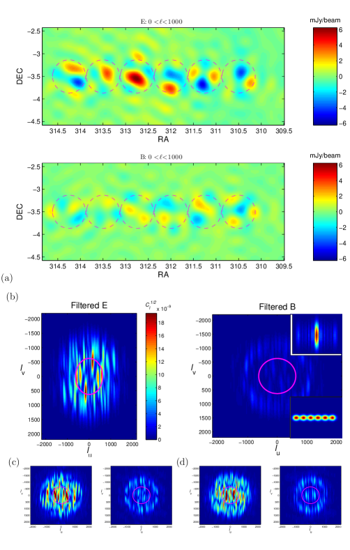
Figure 3: (a) Raw images of the (approximate) E and B signals from the $20^{h}$ deep strip for $\ell<1000$. The circles show the fwhm of each of the six CBI pointings in the strip. A filter has been applied to remove the mean-mode (ground) signal, which would otherwise dominate the maps. No other filters are needed: the raw $20^{h}$ data are dominated by the CMB signal. For the data plotted here, simulations of pure-E and pure-B signals show that the mixing between E and B from sky coverage is $\sim$5% in variance. The E map, which is predominantly signal, has a variance 2.8 times larger than that in the B map (which is consistent with the noise). Because Fourier transforms preserve power, the E/B variance ratio is the same in $\ell$ space. (b) The modulus of the optimal (Wiener-filtered) signal maps seen in the gridded $(\ell_{u},\ell_{v})$-plane using our signal reconstruction process, where $(\ell_{u},\ell_{v})=2\pi(u,v))$. The maps have been normalized to $\sqrt{{\rm{C}}_{\ell}}$, equivalent to plotting $a_{\ell,m}$’s for a full-sky map. The radius of the magenta circles is $\ell=630$, the peak of the CBI’s sensitivity. The EE to BB power ratio in the Wiener-filtered, reconstructed maps is 14.8. The upper inset in the B map is the average mosaic smoothing kernel ${\cal B}$ we chose to smooth the reconstructed maps. The strong anisotropy in $\ell_{u},\ell_{v}$ reflects the geometry of the $20^{h}$ strip. The lower inset is the sky plane representation of $\cal{B}$. (c,d) show two sample maps of the fluctuations $\delta s=s-\langle s|\Delta\rangle$ on the same scale as (b).

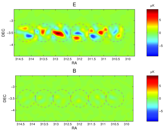
Figure 4: The E and B reconstructed signal sky-plane images of the $20^{h}$ deep strip, the transform of the $\ell$-space images in Fig. 3(b). These should be compared with the raw images in Fig. 3(a).

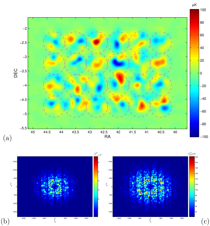
Figure 6: (a) The reconstructed sky image for the Wiener-filtered $02^{h}$ mosaic in total intensity. Both ground and sources (which would otherwise dominate the map) have been removed as part of the filter. This image has been produced using the $uv$-plane CLEAN procedure described in § 2.3. The circles show the fwhm of each of the 24 CBI pointings used in Fig. 5. .(b) The modulus of the optimal (Wiener-filtered) map of (a) in the gridded ($\ell_{u},\ell_{v}$) plane. As in Fig. 5(b), the vertical striping is due to the ground filter. (c) A rescaling of (b) that brings out the structure in the $\ell_{u},\ell_{v}$-plane by multiplying each pixel by $\ell$. This is equivalent to using $\ell(\ell+1)\rm{C}_{\ell}/2\pi$ instead of $\rm{C}_{\ell}$ to plot the angular power spectrum. In this representation, one can see hints of multiple rings of higher signal that correspond to the Doppler peaks in the power spectrum.

3 Parameterized Polarization Phenomenology

3.1 TT, EE, TE and BB Bandpower Data

In our parameter determinations we consider five combinations of bandpower data: (1) CBI TT+EE+TE bandpowers obtained from the analysis described here of the 2002–2005 data with a bin width $\Delta\ell\approx 75$, more fine-grained than those of Table 1 (available as an on-line supplement); (2) CBI $\ell=600$ to $\ell=1960$ TT bands from the combined mosaic and deep field analysis of Readhead et al. (2004a); (3) TT and TE WMAP1 bandpowers from the first year WMAP data (Bennett et al., 2003), adopting the likelihood mapping procedure described in Verde et al. (2003); (4) DASI TT (Kovac et al., 2002) and 3-year EE+TE (Leitch et al., 2004) results; (5) the recent Boomerang B03 TT+EE+TE results (Masi et al., 2005; Jones et al., 2006; Montroy et al., 2006; Piacentini et al., 2006), with $\ell<300$ TT bandpowers excluded because of overlap with WMAP (although this has no quantitative impact). We also omit CBI TT results for $\ell<360$ both because of the overlap with WMAP, and because the (very limited) sensitivity there is coming from the sidelobes of the primary beam which are extremely difficult to measure accurately. The Markov chain Monte Carlo (MCMC) package CosmoMC (Lewis & Bridle, 2002), modified to include polarization spectra, the cross correlation between TT and EE spectra, and isocurvature modes, is used to calculate posterior probability distributions (including priors) for cosmic parameters.

3.2 The Basic Flat Tilted Adiabatic $\Lambda$CDM Model

The simplest inflationary paradigm is characterized by six basic parameters: $\omega_{b}\equiv\Omega_{b}h^{2}$, the physical density of baryons; $\omega_{c}\equiv\Omega_{c}h^{2}$, the physical density of cold dark matter; $\theta\equiv 100\ell_{s}^{-1}$, parameterizing the angular scale $\ell_{s}^{-1}$ associated with sound crossing at decoupling, which defines the overall position of the peak–dip pattern; $\ln(10^{10}A_{s})$, the logarithm of the overall scalar curvature perturbation amplitude $A_{s}$, the scalar curvature power spectrum ${\cal P}_{{\rm s}}(k)$ evaluated at the pivot point $k_{n}=0.05\text{Mpc}^{-1}$; $n_{s}$, the spectral index of the scalar perturbations, defined by ${\cal P}_{{\rm s}}(k)\propto k^{n_{s}-1}$ ; and $\tau$, the Thomson scattering depth to decoupling. We do not consider gravitational-wave induced components.

Table 2 shows the broad priors we have chosen for the basic parameter ranges so that they have little influence on our results. We also impose a weak-$h$ prior on the Hubble constant $H_{0}=100h\,\rm km\,s^{-1}\,Mpc^{-1}$: $0.4<h<1$. For the flat $\Omega_{\rm tot}=1$ models considered here this weak-$h$ prior has little influence on the results, although some extreme models with high Thomson depth are excluded. The strongest prior is the flat restriction, expected in most inflation models. Some parameters change significantly when the flat prior is relaxed (Bond et al., 2003; Readhead et al., 2004a).

We highlight distributions for two parameters, the pattern-shifting $\theta/\theta_{0}$ and $q_{s}=A_{s}e^{-2\tau}/A_{s0}e^{-2\tau_{0}}$ which determines the overall ${\cal C}^{X}_{\ell}$ amplitude. We normalize relative to $\theta_{0}=1.0442$ and $A_{s0}e^{-2\tau_{0}}=18.0\times 10^{-10}$, the best-fit values for WMAP1+CBI+DASI+B03 TT+EE+TE (Table 2). The near-degeneracy between $A_{s}$ and $\tau$ is only weakly broken at very low $\ell$ where reionization has some influence, and at higher $\ell$ through (nonlinear) secondary phenomena such as weak lensing or the Sunyaev-Zeldovich effect. However, the $q_{s}$ combination is reasonably well determined, although there are correlations with other parameters, e.g., $\omega_{b},\omega_{c}$ and $n_{s}$, especially with polarization data only.

The relative positions of the peaks in the TT and EE spectra are “phase-locked” by the physics of the acoustic oscillations at photon decoupling, with the multipole of the $j^{th}$ TT peak $\propto j\theta^{-1}$, and the multipole of the $j^{th}$ EE peak $\propto(j+1/2)\theta^{-1}$. The TE cross-spectrum has double the number of peaks (Fig. 1). For WMAP1+CBI+DASI+B03 TT+EE+TE, we find $\theta/\theta_{0}=1.001\pm 0.0041$ and $q_{s}=0.996\pm 0.037$. For WMAP1+CBI $\theta/\theta_{0}=0.999\pm 0.005$, to be contrasted with the $1.000\pm 0.005$ obtained in Readhead et al. (2004b) for this $\theta_{0}$. These results for the mean values and standard deviations are also very similar to those obtained with other CMB data combinations, e.g., Bond et al. (2003); MacTavish et al. (2006).

For WMAP1+CBI+DASI+B03 TT+EE+TE the other basic cosmic parameters, after marginalization, have distributions shown in Fig. 7 with median values and 1$\sigma$ errors given in Table 2. The best-fit parameters for the fiducial model are also given there. Using WMAP1 TT+TE and CBI+DASI+B03 TT gives very similar results: the inclusion of the current high $\ell$ polarization data has little impact on parameter values for this limited set.

For CBI+DASI+B03 EE+TE, we get $\theta/\theta_{0}$ = $0.986\pm 0.017$ and $q_{s}=0.86\pm 0.14$, in good agreement with the TT result. (A few other parameters are also moderately well constrained, but most are not, as shown in Table 2.) Our $\theta/\theta_{0}$ result is not affected if we relax the flat prior ($0.988\pm 0.018$). For CBI EE $\theta/\theta_{0}$ is $0.986\pm 0.031$ and $q_{s}$ is $1.27\pm 0.48$. For CBI EE+TE $\theta/\theta_{0}$ is $0.95\pm 0.027$ and for DASI+B03 EE+TE it is $1.03\pm 0.030$. For CBI BB we obtain $\theta/\theta_{0}=0.95\pm 0.10$. This should be interpreted as essentially the limit that we would get from the prior probabilities alone. This shows our $\theta/\theta_{0}$ results are data-driven rather than prior-driven.

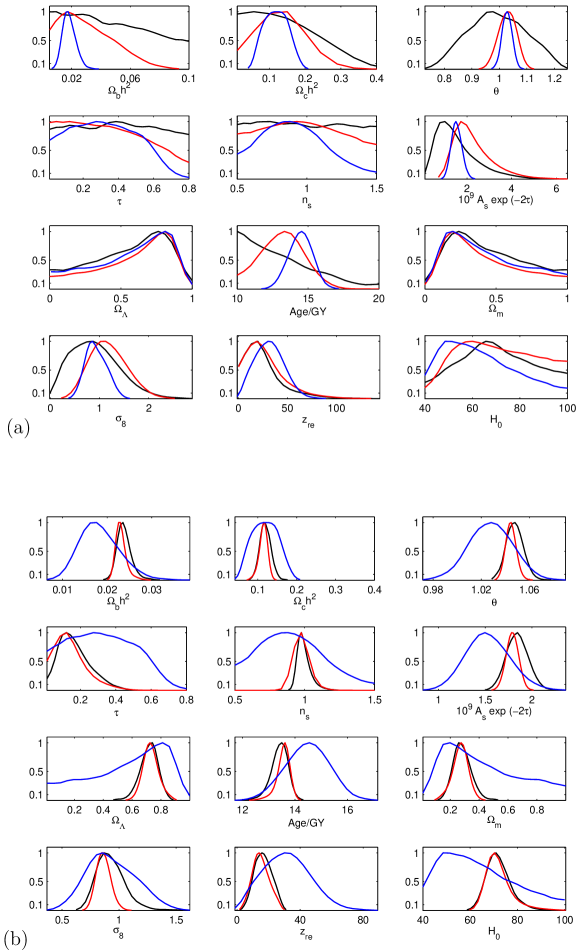
Figure 7: One-dimensional likelihoods for the cosmological parameter indicated, marginalized over the other parameters. (a) shows CBI EE (red), CBI+DASI+B03 EE+TE (blue). The black line is the prior, calculated using a parameter run with CBI BB only. (b) shows WMAP1 only TT+TE (black), WMAP1 TT+TE + CBI+DASI+B03 TT+EE+TE (red) and CBI+DASI+B03 EE+TE (blue).

2 prior WMAP1+CBI+DASI+B03 WMAP1+CBI+DASI+B03 CBI+DASI+B03 range TT+EE+TE (best-fit) TT+EE+TE EE+TE $\theta/\theta_{0}$ 0.5 to 10 1 $1.001\pm 0.0042$ $0.987\pm 0.017$ $\Omega_{b}h^{2}$ 0.005 to 0.1 0.0226 $0.0232\pm 0.0013$ $0.018\pm 0.005$ $\Omega_{c}h^{2}$ 0.01 to 0.99 0.117 $0.114\pm 0.011$ $0.119\pm 0.034$ $\tau$ 0.01 to 0.8 0.105 $0.149\pm 0.086$ $0.33\pm 0.18$ $n_{\rm s}$ 0.5 - 1.5 0.960 $0.978\pm 0.039$ $0.92\pm 0.23$ $\ln[10^{10}A_{\rm s}]$ 2.7 to 4.0 3.09 $3.18\pm 0.16$ $3.37\pm 0.35$ $q_{s}=A_{s}e^{-2\tau}/A_{s0}e^{-2\tau_{0}}$ - 1 $0.992\pm 0.037$ $0.86\pm 0.14$ $\Omega_{\Lambda}$ - 0.714 $0.733\pm 0.054$ $0.58\pm 0.25$ ${\rm Age(Gyr)}$ - 13.6 $13.5\pm 0.26$ $14.4\pm 0.80$ $\Omega_{m}$ - 0.286 $0.267\pm 0.054$ $0.42\pm 0.25$ $\sigma_{8}$ - 0.83 $0.848\pm 0.063$ $0.94\pm 0.21$ $z_{re}$ - 12.5 $15.1\pm 5.3$ $32\pm 15$ $H_{0}$ 40 to 100 70.0 $72.6\pm 5.6$ $64\pm 15$

Table 2: Cosmic parameter values for the flat tilted adiabatic $\Lambda$CDM model

The first group shows the six independent (fitted) parameters, the second group shows parameters derived from them. Mean values and standard deviations are given for TT+EE+TE data in column 4 and for EE+TE in column 5. The ranges for the uniform weak priors we imposed for the MCMC runs are given in column 2. The best-fit model parameters defining our “fiducial model” are shown in column 3. For this model $\theta_{0}=1.0437$ and $A_{s0}e^{-2\tau_{0}}=17.9\times 10^{-10}$. Here These are slightly different than the parameters defining the WMAP team’s best-fit (Spergel et al., 2003) using WMAP1 TT+TE + ACBAR TT + an earlier version of the CBI TT data (Pearson et al., 2003) and different priors: $\Omega_{b}h^{2}=0.0224$, $\Omega_{c}h^{2}=0.111$, $n_{\rm s}(k=0.05)=0.958$, $\tau=0.11$, $H_{0}=72$. This was the fiducial model used in Readhead et al. (2004b). Fig. 1 shows that the two are very similar visually.

3.3 A Peak/Dip Pattern Test

Single-band or broad-band results using theoretically motivated ${\cal C}^{X}_{\ell b}$ shapes can also be produced by our pipeline. These allow complete mapping of the full likelihood surfaces without using the compressed bandpowers. The one-band model ${\cal C}_{\ell}^{X}=q_{s}{\cal C}_{\ell}^{X({\rm s})}$, with ${\cal C}_{\ell}^{X({\rm s})}$ the fiducial adiabatic model, yields for CBI EE $q_{s}=1.02\pm 0.14$ (68%) and a $11.7\,\sigma$ detection relative to $q_{s}=0$; CBI EE+TE gives a $12.4\,\sigma$ detection. These can be compared with the $6.3\,\sigma$ DASI EE detection reported in Leitch et al. (2004) and the $8.9\,\sigma$ CBI EE detection reported in Readhead et al. (2004b) (with no polarization point sources projected out, $7.0\,\sigma$ with 20% removal). Alone, the new CBI TE data give $q_{s}=1.02\pm 0.24$ and a $4.2\,\sigma$ detection relative to $q_{s}=0$. The CBI TT data yield $q_{s}=1.12\pm 0.05$ which is a $95\,\sigma$ significance detection versus $q_{s}=0$.

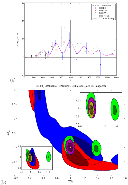
Figure 8: (a) shows the polarization data from CBI, DASI, and B03, along with the fiducial EE prediction (black dashed), the same model shifted by 20% in $\theta$ (black dotted), and the best-fit CBI+DASI+B03 EE cosmology (magenta). The polarization data pick out the same sound-crossing angular scale as the TT data do, with $\theta/\theta_{0}=$ $0.986\pm 0.017$ when marginalized over the other 5 cosmological parameters. (b) shows 1 and 2 $\sigma$ contours derived from CBI EE (green), DASI EE (red), B03 EE (blue) and CBI+DASI+B03 EE (magenta) for the 2-parameter $q_{s}$ and $\theta/\theta_{0}$ template model. Marginalization yields $\theta/\theta_{0}=0.993\pm 0.027$, $q_{s}=1.00\pm 0.11$. The yellow star marks the expected result from the fiducial model. The lower inset shows the same with EE+TE instead of EE only. The upper inset shows the sequence CBI EE (green), CBI+DASI+B03 EE (magenta), CBI+DASI+B03 EE+TE (brown). Marginalization yields $\theta/\theta_{0}=0.988\pm 0.018$, $q_{s}=0.97\pm 0.09$. Grey contours denote CBI+B03 TT.

To further complement the MCMC determinations, we consider the two-parameter template model ${\cal C}_{\ell}^{X}=q_{s}{\cal C}_{\ell(\theta_{0}/\theta)}^{X({\rm s})}$, evaluated on a grid in $(q_{s},\theta/\theta_{0})$. The other cosmic parameters are fixed at the fiducial model values. We restrict $\theta/\theta_{0}$ to lie between $0.3$ and $1.7$, the range of our grid. Fig. 8(a) shows how the EE peak/dip pattern shifts for the polarization. The $\theta/\theta_{0}$–$q_{s}$ likelihood contours in Fig. 8(b,c,d) show that for each of the EE polarization datasets there is a multimodal probability structure. For example, for CBI, apart from the $\theta/\theta_{0}\approx 1$ solution, there is another with the third polarization peak shifted and scaled to fit the second peak of the fiducial model. There is a strong probability minimum in between the two. This multiple solution disappears when DASI and B03 are combined with CBI, yielding the well-determined $\theta/\theta_{0}=0.988\pm 0.018$, $q_{s}=0.97\pm 0.09$ for EE+TE. These are in good agreement with the $0.986\pm 0.017$ and $q_{s}=0.86\pm 0.14$ MCMC numbers determined by marginalizing over the other five cosmic parameters. The multimodal aspect is strongly suppressed in MCMC just because of the extremely weak-$h$ prior we impose, but correlations among parameters lead to the larger errors in $q_{s}$. For EE alone, the template grid gives $\theta/\theta_{0}=0.993\pm 0.027$, $q_{s}=1.00\pm 0.11$ and the marginalized MCMC gives $\theta/\theta_{0}=1.003\pm 0.027$, $q_{s}=1.07\pm 0.30$.

Fig. 8 shows the best-fit EE+TE power spectrum. It looks remarkably like the TT fiducial model forecast.

3.4 Adding a Subdominant Isocurvature Mode

Isocurvature modes which could lead to a measurable signal in the CMB may arise in multiple scalar field models during inflation or they can be generated after inflation has ended. Necessary ingredients to impact CMB and large scale structure (LSS) observations include: association with a component of significant mass-energy, such as baryons, cold dark matter, or, possibly, massive neutrinos (hot dark matter); sufficiently large primordial fluctuations in the entropy-per-baryon, the entropy-per-CDM-particle or the entropy-per-neutrino. A concrete CDM realization is the axion. For cosmic-defect-induced isocurvature perturbations, which could also arise near the end of or after inflation, the mass-energy is in the defects.

Isocurvature perturbations from quantum zero point fluctuations in inflation have a well-defined pattern (Efstathiou & Bond, 1986; Bond & Efstathiou, 1987) in TT, EE and TE, with no BB predicted (except through lensing). The peaks and dips are predicted to be out of phase with those from adiabatic modes, as shown in Fig. 9. (For defects it is difficult to get any peaks and troughs at all.) Further, there is a large “isocurvature effect” predicted at lower $\ell$ relative to that at high $\ell$ where the peaks are.

A pure isocurvature mode does not fit the current TT data unless the primordial isocurvature power spectrum ${\cal P}_{{\rm iso}}(k)$ is designed to mimic the observed ${\cal C}^{{\rm TT}}_{\ell}$ pattern with its own peak/dip structure and overall $k$-dependent blue tilt. Although highly baroque in terms of inflation models, such radically broken scale invariance is possible for isocurvature perturbations just as it is for the adiabatic case. Polarization (and LSS) data help by breaking such severe degeneracies with the cosmic parameters.

A detailed analysis of a general set of isocurvature initial conditions for four cosmological fluids using CMB and LSS data has been undertaken in Moodley et al. (2004). If one includes all allowed isocurvature and adiabatic perturbations, and correlations between them, the current CMB and LSS data still allow a substantial amount of isocurvature perturbations. However simpler and more realistic models that only include an isocurvature perturbation in one fluid are more strongly constrained.

Here we assume Gaussian-distributed CDM isocurvature perturbations and add two extra parameters beyond our base adiabatic six: two amplitude ratios, $R_{i}\equiv{\cal P}_{{\rm iso}}(k_{i})/{\cal P}_{{\rm s}}(k_{i})$, at two pivot wavenumbers $k_{i}$, one at small scale, $k_{2}=k_{n}=0.05\text{Mpc}^{-1}$ and one at large scale, $k_{1}=0.005\text{Mpc}^{-1}$. A (constant) primordial spectral index defined by ${\cal P}_{{\rm iso}}(k)\propto k^{n_{iso}}$ follows: $n_{\rm iso}$ = $n_{\rm s}-1+\ln(R_{2}/R_{1})/\ln(k_{2}/k_{1})$.

We find that for neither $R_{i}$ parameter is there evidence for an isocurvature detection, in agreement with MacTavish et al. (2006) who used the same $R_{1}$–$R_{2}$ parameterization. We find for WMAP1+CBI+DASI+B03 TT+EE+TE, 95% confidence upper limits of $R_{1}$ $<0.26$ and $R_{2}<1.7$ on the higher wavenumber scales which CBI probes. This translates into steeper $n_{\rm iso}$ values being more allowed than the $n_{\rm iso}\approx 0$ nearly scale invariant ones. The CBI EE+TE data only limits $R_{1}<18$ and $R_{2}<54$, whereas CBI+DASI+B03 EE+TE gives $R_{1}<9$ and $R_{2}<30$.

Inflation models more naturally produce nearly scale invariant isocurvature spectra, with $n_{\rm iso}\approx 0$, just as one often gets $n_{\rm{s}}\approx 1$ for adiabatic perturbations. The tilts from theory are also more likely to be red ($n_{iso}<0$) than blue ($n_{iso}>0$). However the data more strongly constrain red models than blue.

3.5 Constraints on Interloper Isocurvature Peaks

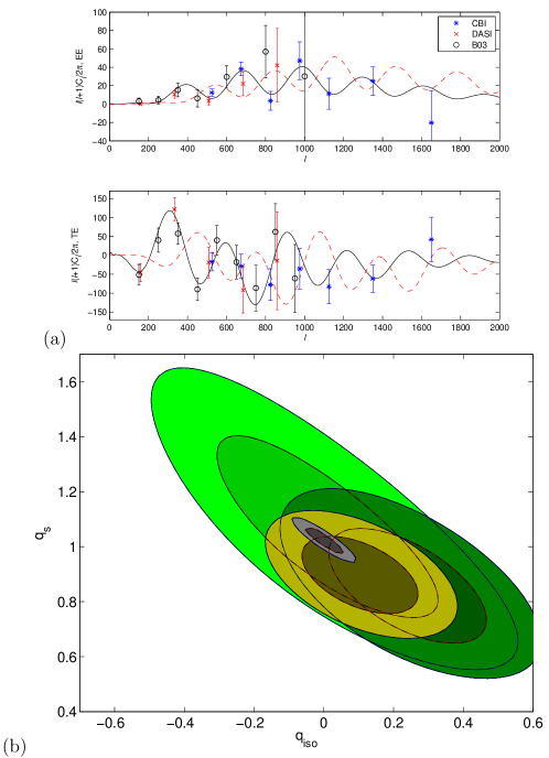
Figure 9: (a) ${\cal C}^{{\rm EE}({\rm iso})}_{\ell}$ and ${\cal C}^{{\rm TE}({\rm iso})}_{\ell}$ power spectra for the $n_{iso}=3$ white noise isocurvature model (red dashed) are compared with ${\cal C}^{{\rm EE}({\rm s})}_{\ell}$ and ${\cal C}^{{\rm TE}({\rm s})}_{\ell}$ for the best-fit adiabatic fiducial model (black). These are the template spectra used for the 2-parameter $q_{s}$-$q_{iso}$ test. $q_{iso}$ is normalized to give the fraction of the expected EE power that is observed in the data over the range $400\leq\ell\leq 1200$. The CBI (blue asterisks), DASI (red x’s) and B03 (black circles) EE and TE data are also shown. (b) The likelihood surface for the 2-parameter $q_{s}$-$q_{iso}$ model, for the CBI EE (light green), CBI EE+TE (dark green), CBI+DASI+B03 EE+TE (brown), and CBI+B03 TT (grey) data. The data strongly prefer the adiabatic over the isocurvature spectrum. Marginalization over the 2D distributions yields: for CBI EE $q_{s}=1.05\pm 0.22$, $q_{iso}=-0.01\pm 0.21$; for CBI TE $q_{s}=0.81\pm 0.24$, $q_{iso}=0.49\pm 0.26$; and for CBI+DASI+B03 EE+TE data $q_{s}=0.90\pm 0.10$, $q_{iso}=0.10\pm 0.11$. The polarization data are consistent with a single component adiabatic inflation model.

To focus attention on the high $\ell$ polarization results, we now fix $n_{\rm iso}$ to be the extremely blue 3, the white noise ‘isocurvature’ spectrum, with no spatial correlation. Large angular scales in ${\cal C}^{X(iso)}_{\ell}$ are highly suppressed and the isocurvature peaks and troughs emerge looking somewhat like an $\ell$-shifted version of the adiabatic spectrum, as shown in Fig. 9. (The $n_{iso}=2$ case, which looks even more like a shifted version of the fiducial model, gives similar results to those given here. See MacTavish et al. (2006) for a treatment of both $n_{iso}=2$ and $3$ cases.) Although ${\cal P}_{iso}(k)$ is so steep for such blue spectra that it must be regulated by a cutoff at high $k>>k_{2}$, ${\cal C}^{X(iso)}_{\ell}$ has a larger natural damping scale so we do not need to add another parameter.

The 2-parameter template model, ${\cal C}^{X}_{\ell}=q_{s}{\cal C}^{X({\rm s})}_{\ell}+q_{iso}{\cal C}^{X({\rm iso})}_{\ell}$, therefore tests at what level an interloper set of isocurvature peaks would be allowed by the CMB data which, as we have seen in the $\theta/\theta_{0}$ test, prefer the adiabatic peak positions. We normalize $q_{iso}$ so that $q_{iso}=1$ corresponds to the same power in ${\cal C}^{{\rm EE}({\rm iso})}_{\ell}$ as in ${\cal C}^{{\rm EE}({\rm s})}_{\ell}$ over a band from $\ell=400$ to $1200$. We find $q_{iso}\approx R_{2}q_{s}/80$. Fig. 9(b) shows a strong preference for the pure adiabatic mode and no isocurvature detection, with $q_{iso}=-0.01\pm 0.21$ for CBI EE, $0.24\pm 0.15$ for CBI EE+TE and $0.10\pm 0.11$ for all of the polarization data.

We also let the full 7 cosmological parameters vary, using CosmoMC to evaluate the probability distribution for $R_{2}$. This is a different exercise than the 2-parameter case: to match the data, the other parameters are adjusted by CosmoMC to make the isocurvature troughs and peaks interfere with the adiabatic peaks and troughs, respectively, to mimic no interloping at all. For CBI EE+TE we get $R_{2}<76$ whereas for CBI+DASI+B03 EE+TE we get $R_{2}<44$. For WMAP1+CBI+DASI+B03 TT+EE+TE, we get $R_{2}<3.0$. We note that ${\cal C}_{B}^{{\rm TT}({\rm iso})}/{\cal C}_{B}^{{\rm TT}({\rm s})}\sim R_{2}/80$, the same as for the EE ratio. Thus the upper limits correspond to an allowed CMB contamination of this subdominant component of only $\sim 3\%$. For EE+TE, $q_{iso}=0.16\pm 0.21$ with an upper limit of 55%, similar to the template value.

4 Conclusions

In this paper we present the results from 2.5 years of dedicated polarization-optimized measurements with the Cosmic Background Imager. From this data, we estimate the TT, TE, EE and BB CMB angular power spectra. The EE power spectrum gives us a 11.7$\sigma$ detection of polarization, the strongest thus far, while TE is measured at 4.2$\sigma$ versus zero. The BB spectrum gives a 95% confidence upper limit of $3.8\,\mu\rm{K}^{2}$.

We introduce a novel method for the reconstruction of $\ell$-space maps of $\tilde{E}$ and $\tilde{B}$. Images of the E and B fields on the sky are formed by Fourier transform of the $\ell$-space maps; this is a new way of representing CMB polarization and is complementary to the standard Stokes Q and U images shown previously in Readhead et al. (2004b). The E-mode detection and the lack of one in B is evident in both the raw maps and the reconstructed Wiener-filtered images of the $20^{h}$ strip and is also evident in the square mosaic fields. We have also verified that signal-map fluctuations, shown in Fig. 4(c,d), about the mean signal in Fig. 4(b) do not obscure this clear detection: the $20^{h}$ strip is indeed dominated by the CMB polarization signal. The signal maps of the total intensity, an example of which is shown in Fig 6 for the $02^{h}$ mosaic, also show very strong detections.

An analysis of a six-dimensional space of cosmological parameters shows that the patterns and amplitudes in the EE, TE and BB data are entirely consistent with the basic inflation-based model predictions from TT, a result considerably strengthened by the new CBI EE+TE data. The combined CBI+DASI+B03 EE+TE data further sharpens this conclusion. This is particularly evident in Fig. 8 which shows that $\theta/\theta_{0}$, parameterizing the angular scale associated with sound crossing at decoupling and hence the peak-dip pattern, is pinned down to the value we obtain from TT alone.

We finally explore a restricted physically-motivated class of models with combined, but uncorrelated, adiabatic and isocurvature perturbations. We find that there is effectively no evidence for an isocurvature mode in the data. Furthermore the data rule out a possible family of interloper peaks which would be out of phase with the standard flat adiabatic predictions. This strengthens our claim that cosmological models with an additional isocurvature mode are disfavored by the current polarization data.

References

- Barkats et al. (2005) Barkats, D. et al. 2005, Astrophys. J., 619, L127
- Bennett et al. (2003) Bennett, C. et al. 2003, Astrophys. J. Suppl., 148, 97
- Bond et al. (2003) Bond, J. R., Contaldi, C. R., & Pogosyan, D. 2003, Phil. Trans. Roy. Soc. Lond., A361, 2435
- Bond & Efstathiou (1984) Bond, J. R. & Efstathiou, G. 1984, Astrophys. J. Lett., 285, 45
- Bond & Efstathiou (1987) —. 1987, Mon. Not. Roy. Astron. Soc., 226, 655
- Bond et al. (2000) Bond, J. R., Jaffe, A. H., & Knox, L. E. 2000, Astrophys. J., 533, 19
- Bunn et al. (2003) Bunn, E. F., Zaldarriaga, M., Tegmark, M., & Oliveira-Costa, A. d. 2003, Phys. Rev., D67, 023501
- Cartwright et al. (2005) Cartwright, J. K. et al. 2005, Astrophys. J., 623, 11
- Efstathiou & Bond (1986) Efstathiou, G. & Bond, J. R. 1986, Mon. Not. Roy. Astron. Soc., 218, 103
- Högbom (1974) Högbom, J. A. 1974, A&AS, 15, 417
- Jones et al. (2006) Jones, W. et al. 2006, ApJ, 647, 823
- Kogut et al. (2003) Kogut, A. et al. 2003, Astrophys. J. Suppl., 148, 161
- Kovac et al. (2002) Kovac, J. et al. 2002, Nature, 420, 772
- Leitch et al. (2004) Leitch, E. M. et al. 2004, Astrophys. J., 624, L10
- Lewis & Bridle (2002) Lewis, A. & Bridle, S. 2002, Phys. Rev., D66, 103511
- Lewis et al. (2002) Lewis, A., Challinor, A., & Turok, N. 2002, Phys. Rev. D, 65, 023505
- MacTavish et al. (2006) MacTavish, C. et al. 2006, ApJ, 647, 799
- Masi et al. (2005) Masi, S. et al. 2005, submitted to Astron Ap (astro-ph/0507509)
- Montroy et al. (2006) Montroy, T. et al. 2006, ApJ, 647, 813
- Moodley et al. (2004) Moodley, K., Buchler, M., Dunkley, J., Ferreira, P. G., & Skordis, C. 2004, Phys. Rev., D70, 103520
- Myers et al. (2003) Myers, S. T. et al. 2003, Astrophys. J., 591, 575
- Padin et al. (2002) Padin, S. et al. 2002, Pub. Ast. Soc. Pac., 114, 83
- Pearson et al. (2003) Pearson, T. J. et al. 2003, Astrophys. J., 591, 556
- Piacentini et al. (2006) Piacentini, F. et al. 2006, ApJ, 647, 833
- Readhead et al. (2004a) Readhead, A. C. S. et al. 2004a, Astrophys. J., 609, 498
- Readhead et al. (2004b) —. 2004b, Science, 306, 836
- Sievers et al. (2003) Sievers, J. L. et al. 2003, Astrophys. J., 591, 599
- Spergel et al. (2003) Spergel, D. N. et al. 2003, Astrophys. J. Suppl., 148, 175
- Tucci et al. (2004) Tucci, M., Martinez-Gonzalez, E., Toffolatti, L., Gonzalez-Nuevo, J., & De Zotti, G. 2004, Mon. Not. Roy. Astron. Soc., 349, 1267
- Verde et al. (2003) Verde, L. et al. 2003, Astrophys. J. Suppl., 148, 195