The Multiwavelength Survey by Yale-Chile (MUSYC): Survey Design and Deep Public UBVRIz^′ Images and Catalogs of the Extended Hubble Deep Field South

Abstract

We present $UBVRIz^{\prime}$ optical images taken with CTIO4m+MOSAIC of the 0.32 deg² Extended Hubble Deep Field South. This is one of four fields comprising the MUSYC survey, which is optimized for the study of galaxies at $z=3$, AGN demographics, and Galactic structure. Our methods used for astrometric calibration, weighted image combination, and photometric calibration in AB magnitudes are described. We calculate corrected aperture photometry and its uncertainties and find through tests that these provide a significant improvement upon standard techniques. Our photometric catalog of 62968 objects is complete to a total magnitude of $R_{\rm AB}=25$, with $R$-band counts consistent with results from the literature. We select $z\simeq 3$ Lyman break galaxy (LBG) candidates from their $UVR$ colors and find a sky surface density of 1.4 arcmin^-2 and an angular correlation function $w(\theta)=2.3\pm 1.0\theta^{-0.8}$, consistent with previous findings that high-redshift Lyman break galaxies reside in massive dark matter halos. Our images and catalogs are available at http://www.astro.yale.edu/MUSYC.

1. INTRODUCTION

The study of galaxy formation and evolution requires detailed information about statistically significant samples of dim objects. This, in turn, requires deep imaging and spectroscopy over wide areas of the sky. In pursuit of these data, several wide-deep surveys are now underway. Those covering several square degrees or more either lack spectroscopic follow-up (e.g. NOAO DWFS, Jannuzi & Dey 1999, and ODTS, MacDonald et al. 2004) or are restricted to the study of objects at $z\lesssim 1$ (except for quasars) by their imaging depth e.g. the Sloan Digital Sky Survey (York et al. 2000 and Abazajian et al. 2005), the VIRMOS-VLT Deep Survey (Le Fèvre et al. 2004, Radovich et al. 2004) and DEEP2 (Davis et al., 2003). Other surveys target the high-redshift universe with deep HST imaging over fractions of a square degree i.e. the Hubble Deep Fields (Williams et al., 1996, 2000), the Hubble Ultra Deep Field (HUDF), GOODS (Giavalisco et al., 2004; Dickinson et al., 2004), and GEMS (Rix et al., 2004). Spectroscopic coverage is feasible over these areas but is presently unable to probe deeper than $R\simeq 25$, making the added imaging depth useful only for morphological studies and photometric redshifts.

The Multiwavelength Survey by Yale-Chile (MUSYC) probes the intermediate regime of a square degree of sky to the spectroscopic limit of $R\simeq 25$. Section 2 describes the design of our survey. §3 reports our imaging observations for the extended Hubble Deep Field South. §4 describes our imaging reduction, and §5 covers our photometric calibration and photometry. §6 gives our results for $R$-band number counts and the sky density and angular clustering of $UVR$-selected Lyman break galaxies. §7 concludes. Our analyses assume a standard $\Lambda$CDM cosmology with $\Omega_{m}$=0.27,$\Omega_{\Lambda}=0.73$, and $H_{0}$=70km/s/Mpc.

2. SURVEY DESIGN

The Multiwavelength Survey by Yale-Chile (see http://www.astro.yale.edu/MUSYC) is designed to provide a fair sample of the universe for the study of the formation and evolution of galaxies and their central black holes. The core of the survey is a deep imaging campaign in optical and near-infrared passbands of four carefully selected $30^{\prime}\times 30^{\prime}$ fields. MUSYC is unique for its combination of depth and total area, for additional coverage at X-ray, UV, mid- and far-infrared wavelengths and for providing the $UBVRIz^{\prime}JHK$ photometry needed for high-quality photometric redshifts over a square-degree of sky. The primary goal is to study the properties and interrelations of galaxies at a single epoch corresponding to redshift $\sim 3$, using a range of selection techniques. We chose to use the $UBVRIz^{\prime}$ filter set in the optical in order to obtain six nearly-independent flux measurements with the broadest possible wavelength coverage.

Lyman break galaxies at $z\simeq 3$ are selected through their dropout in $U$-band images combined with blue continuua in $BVRIz^{\prime}$ ($\lambda>1216$Å in the rest-frame) typical of recent star formation (Steidel et al., 1996b, 1999, 2003). Imaging depths of $U$,$B$,$V$,$R\simeq 26$ were chosen to detect the LBGs, whose luminosity function has a characteristic magnitude of $m_{*}=24.5$ in $R_{\mathrm{A}B}$, and to find their Lyman break decrement in the $U$ filter via colors $(U-V)_{\mathrm{A}B}>1.2$.

Lyman $\alpha$ emitters at $z\simeq 3$ are selected through additional deep narrow-band imaging using a 50Å fwhm filter centered at 5000Å. These objects can be detected in narrow-band imaging and spectroscopy by their emission lines, allowing us to probe to much dimmer continuum magnitudes than possible for Lyman break galaxies.

It has recently become clear that optical selection methods do not provide a full census of the galaxy population at $z\sim 3$, as they miss objects which are faint in the rest-frame ultraviolet (Franx et al., 2003; Daddi et al., 2004). With this in mind, MUSYC has a comprehensive near-infrared imaging campaign. The NIR imaging comprises two components: a wide survey covering the full square degree and a deep survey of the central $10^{\prime}\times 10^{\prime}$ of each field. This division between deep and wide was chosen because of the $10.5^{\prime}$ field-of-view of the ISPI near-infrared camera on the CTIO 4m telescope. The $5\sigma$ point source sensitivities of the wide and deep components are $K_{s,AB}=22.0$ and $K_{s,AB}=23.3$ respectively. NIR imaging over the full survey area provides a critical complement to optical imaging for breaking degeneracies in photometric redshifts and modeling star formation histories. Deeper $JHK_{s}$ imaging over $10^{\prime}\times 10^{\prime}$ subfields opens up an additional window into the $z\simeq 3$ universe as the $J-K$ selection technique (Franx et al., 2003; van Dokkum et al., 2003, 2004) will be used to find evolved optically-red galaxies at $2<z<4$ through their rest-frame Balmer/4000Å break.

Extensive follow-up spectroscopy is being conducted over the square degree. A subset of the color-selected Lyman break galaxy candidates will turn out to be AGN based on broad- or narrow-line emission features seen in follow-up spectroscopy (Steidel et al., 2002). Damped Lyman $\alpha$ Absorption systems (Wolfe et al., 1986) at $z>2.3$, which comprise the neutral gas reservoir needed to form most of the stars in the universe (Wolfe et al., 2005), will be searched for in the spectra of the brightest color-selected LBG/AGN candidates (typically quasars at $z\sim 3$).

In addition to the optical and near-infrared, imaging campaigns at other wavelengths and follow-up spectroscopy are integral parts of MUSYC. X-ray selection will be used to study AGN demographics over the full range of accessible redshifts, $0<z<6$, (see Lira et al., 2004) with Spitzer imaging used to detect optically- and X-ray-obscured AGN (Treister et al., 2004; Lacy et al., 2004). This also allows a census of accreting black holes at $z\simeq 3$ in the same fields to study correlations between black hole accretion and galaxy properties at this epoch.

Future epochs of optical imaging will be used to conduct a proper motion survey to find white dwarfs and brown dwarfs in order to study Galactic structure and the local Initial Mass Function (see Altmann et al., 2004); the additional epochs will also enable a variability study of AGN.

The four survey fields (see Table 1) were chosen to have extremely low reddening, HI column density (Burstein & Heiles, 1978), and 100$\mu$m dust emission (Schlegel et al., 1998) in order to facilitate satellite coverage with Spitzer, HST, Chandra, and XMM, to take advantage of existing multiwavelength data and to enable flexible scheduling of observing time during the year. Additionally, each field satisfies all of the following criteria: minimal bright foreground sources in the optical and radio, high Galactic latitude ($|b|>30$) to reduce stellar density, and accessibility from observatories located in Chile. The survey fields will be a natural choice for future observations with ALMA.

The remainder of this paper describes our optical images and catalog of E-HDFS. The techniques used for data reduction and photometry are the same as those used for the analysis of the other three fields. Optical imaging from the full survey will be reported in E. Gawiser et al. (2005, in preparation). The near-infrared data will be discussed in R. Quadri et al. (2005, in preparation). The E-HDFS has deep public space-based observations at UV, optical, near-infrared, and far-infrared wavelengths. The HDFS itself covers a small $\sim 2.5^{\prime}\times 2.5^{\prime}$ central region with WFPC2 plus STIS and NICMOS regions, with deep ground-based JHK coverage of the WFPC2 region available from the FIRES survey (Labbé et al., 2003). Spitzer IRAC and MIPS coverage of the central $5^{\prime}\times 15^{\prime}$ is being performed in GTO time. The extended area around HDFS has previously been imaged by Palunas et al. (2000) and Teplitz et al. (2001) to a depth sufficient for the study of galaxies at $z<1$. These images were made public and combined with deep H-band images by the Las Campanas Infrared Survey (LCIRS, Chen et al. 2002) to study red galaxies out to $z\simeq 1.5$. Our survey goes about one magnitude deeper in UBVRI$z^{\prime}$ to probe the $z=3$ universe. Our Extended Hubble Deep Field South (E-HDFS) field center (see Table 1) was chosen to keep a bright star (m=6.8) which lies just North of the WFPC2 field off of the CTIO+MOSAIC detectors. LCIRS covered an H-shape centered on WFPC2 and thereby provides public $H$-band coverage of roughly half of our E-HDFS field.

3. OBSERVATIONS

Optical images of E-HDFS were taken on the nights of 2002 October 6,8,10,12 and 2003 May 26,27,28 using the 8192$\times$8192 pixel MOSAIC II camera consisting of 8 2048$\times$4096 CCDs, each with 2 amplifiers, on the Blanco 4m telescope at CTIO. Afternoon calibrations were obtained, including zero-second exposures to trace the readout bias pattern, and domeflats in each filter to be observed except for $U$ for which the counts from the dome lamps were insufficient. Twilight flats were therefore obtained for the $U$ filter. Dark exposures of comparable length to the imaging observations were obtained, but due to the negligible dark current they were not used for data reduction. A standard dither pattern was used to fill in gaps between the 8 CCDs. The pixel scale is 0.267^′′/pixel, leading to coverage spanning $37^{\prime}\times 37^{\prime}$ of sky with each pointing. Figure 1 shows the filter response curves and their multiplication with the CCD quantum efficiency and atmospheric transmission at one airmass. Table 2 gives details of the exposure times in each filter for each run along with the approximate average seeing measured in the raw images during observations. The seven nights were mostly cloudless, but moderate clouds affected some of the $V$ imaging of E-HDFS on 2002 October 10,12 and some of the $R$ imaging on 2003 May 28; our reduction methods described below allow these images to be used without biasing the photometry. Photometric standard fields from Landolt (1992) large enough to cover the full MOSAIC II field of view were observed each night, and the nights of 2002 October 6 and 2003 May 26 proved photometric.

Figure 1.— MOSAIC II $UBVRIz^{\prime}$ filter set, starting with $U$ at left. Dotted lines show filter throughput, and solid lines show total system throughput after multiplying by CCD quantum efficiency and atmospheric transmission at one airmass.

4. DATA REDUCTION

$UBVRIz^{\prime}$ images from CTIO4m+MOSAIC II were reduced using the MSCRED and MSCDB packages in IRAF v.2.12 following the NOAO Deep Wide Field Survey cookbook v.7.02. We used custom software to work around a few difficulties in these packages, as described below.

A composite zero image is subtracted from each raw image to remove the amplifier bias level and pattern. The resulting image is then “flat-fielded” by dividing by a composite domeflat, or a composite twilight flat in the case of $U$-band. A superskyflat for each filter is made by combining all of the flat-fielded, unregistered images taken in each filter each night with rejection used to remove sources. Our 2^′ amplitude dither pattern was designed to eliminate the wings of bright sources from the superskyflat. Each flat-fielded image is then divided by the appropriate superskyflat, which offers an estimate of the pixel-by-pixel response to the spectrum of the night sky with sufficient counts to achieve 1% precision per pixel. Because the superskyflat was produced using flat-fielded images, dividing by it serves to remove the original domeflat (twilight flat) from the reduction process. The real influence of the original flat-fielding is to remove the illumination pattern and gross pixel-to-pixel variations before looking for cosmic rays and bright objects to reject in making the superskyflat. Using the superskyflat to correct for the pixel response is considered preferable to using the domeflat because the CCD response to the spectrum of the dome lamp (or twilight sky) can have significant systematic differences from its response to the spectrum of the night sky. For background-limited photometry, this is an important effect.

We then find an astrometric solution for each image, starting with fiducial WCS headers provided for each fits extension of the raw images and comparing the claimed positions with the known positions of stars in the USNO-B catalog using the MSCRED routine msccmatch. We found msccmatch to be finicky; for some runs the fiducial headers were too inaccurate to be corrected with the maximum second-order terms used by the MSCRED package. An iterative, non-interactive procedure of calling msccmatch multiple times proved sufficient. The final rms astrometric errors are between 0.2^′′ and 0.3^′′ in each image, which is consistent with the uncertainties on individual USNO-B stars despite having fit many more stars than free parameters, and the actual solution should be better than 0.2^′′ rms.

To perform aperture photometry later on, our final images are transformed to have a common pixel scale and tangent plane projection point. This is accomplished by projecting each processed image (after bias-subtraction, flat-fielding, superskyflat-fielding, and correction of WCS header information) onto the tangent plane of a common reference image using mscimage. The reprojection performed by mscimage should be performed with flux conservation set to no the first time but then set to yes for any further reprojections. This is because the pixel scales in raw MOSAIC II images are a function of radius from the field center with several percent variation from center to corner of the field. The process of flat-fielding removes the true illumination pattern caused by more photons falling in larger pixels leading to an illusion of flat background counts despite the variation in pixel scales. When mscimage is used for astrometric projection into a uniformly sized grid of pixels, flux conservation would re-introduce the illumination pattern, thereby causing a variable photometric zeropoint across the image. Turning off flux conservation instead produces an average of the values of initial pixels neighboring each final pixel location that offsets the error introduced by flat-fielding.

We make three different stacked “final” images for each filter. Unweighted versions are made first in order to determine the weights for the other two versions. The versions denoted by xs were combined using weights optimized for surface brightness, which is the method used by the NDWFS cookbook. The versions denoted by ps were made using weights optimized for point sources; details can be found in the Appendix.

We synthesize a $BVR$_ps image to use as our photometric detection image by adding the $B$, $V$, and $R$ ps stacks using point-source-optimized weights derived from the signal and noise statistics of these stacks. We decided not to add $U$ to $BVR$ although it is also very deep because some low-redshift objects have different morphologies in $U$, the seeing is typically worse in $U$, and objects at $z\simeq 3$ will be nearly invisible in $U$ so adding it to $BVR$ would just add noise for these objects. Note that for similar reasons objects that drop out in $B$ and $V$ are somewhat less likely to be detected in our $BVR$ image than in a $VR$ or $R$ image alone. We prefer the $BVR$ approach to the creation of a $\chi^{2}$ image advocated by Szalay et al. (1999) because it allows us to measure object morphological parameters directly from the same image used for object detection, which is not recommended in the latter approach. Moreover, the optimally-weighted $BVR$ combination reduces the emphasis on single-filter outliers employed by the $\chi^{2}$ approach and avoids its flaw of treating both negative and positive sky fluctuations as evidence of an object.

We trim the final $BVR$_ps image to the maximum size region that has nearly uniform signal-to-noise ratio in all three input images $B$, $V$, and $R$. For E-HDFS, the trimmed image is 7395$\times$7749 pixels or $33^{\prime}\times 34.5^{\prime}$. Then the IRAF task imalign is used to shift and trim the other images to match, giving our images the common origin and size required for aperture photometry with SExtractor. The trimmed images are normalized to an effective exposure time of one second. After the pipeline reduction, the background is flat to better than 1% in all filters. The remaining low level, large scale fluctuations were subtracted using SExtractor (Bertin & Arnouts, 1996) with mesh size BACK_SIZE=64 and median filter BACK_FILTERSIZE set to 6 mesh units.

Figure 2.— $33^{\prime}\times 34.5^{\prime}$ combined $BVR$ image of E-HDFS used for object detection. The mild background feature at the top just left of center is caused by the reflection of a magnitude 6.8 star just outside the field.

The resulting final $BVR$ image is shown in Figure 2 with a magnified image of a small section shown in Fig. 3. New FITS headers have been added to these final images indicating input information for SExtractor photometry runs and other routines, specifically:
SATUR_LEVEL, the empirically determined saturation level in each image, which is usually a factor of a few less than the apparent saturation level of the brightest stars,
SEEING_FWHM, the mode of the seeing for a set of bright unsaturated stars,
MAG_ZEROPOINT, the AB magnitude of an object that gives 1 count per second derived from photometric calibration as described below,
FLUX_ZEROPOINT, the flux in $\mu$Jy corresponding to 1 count per second,
TOT_EXPTIME, the total exposure time that each final image represents, and
GAIN_TOT, the number of photoelectrons represented by each count in the final image.

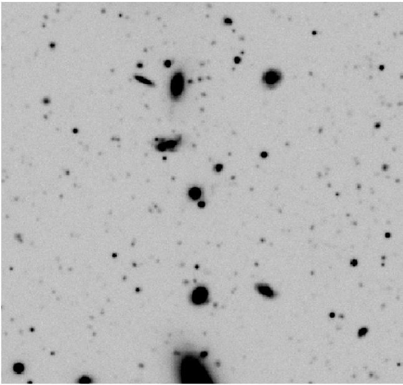
Figure 3.— $2^{\prime}\times 2^{\prime}$ zoom of $BVR$ detection image. The seeing in the image is 0.95^′′ fwhm.

5. PHOTOMETRY

5.1. Photometric Calibration

Our calibration scheme is to take $\sim$5 minute exposures of our fields (referred to as “calibration images”) in all optical filters on photometric nights. This was achieved for E-HDFS on Oct. 6, 2002. Photometric calibration is performed using a version of the Landolt catalog with all magnitudes and colors converted into the AB95 system of Fukugita et al. (1996) (referred to throughout this paper as AB magnitudes). We included $z^{\prime}$ magnitudes for Landolt standard stars in our catalog of standards using the formula

$$z^{\prime}_{\mathrm{A}B}=I_{\mathrm{A}B}-0.59(R-I)_{\mathrm{A}B}+0.16(V-R)_{\mathrm{A}B}-0.04\;\;\;,$$ (1)

which was generated from the formulae of Fukugita et al. (1996) and has been corrected for a 0.02 magnitude bias found when comparing this prediction with measurements of $z^{\prime}$ magnitudes of bright Landolt stars by Smith et al. (2002). The resulting 0.04 magnitude rms error was used to predict errors in these estimates. This procedure offers a significant reduction in observing time and a tremendous increase in the number of calibration stars versus the traditional method of using spectrophotometric standard stars for filters outside the Johnson-Cousins system. Only a few stars per Landolt field have been turned into SDSS calibrators (Smith et al., 2002) and they are typically too bright for the 4m telescope to use without defocusing.

Table 3 lists the airmass and seeing for each of our calibration images along with our photometric solution for the magntiude in terms of measured counts per second,

$$m=-2.5\log_{10}(counts/s)+Z-cX-Colorterm\;\;\;,$$ (2)

where $Z$ is the magnitude zeropoint, $c$ is the airmass coefficient, $X$ is airmass, and the color term is listed in Table 3. Our images of Landolt standard fields occupied a range of airmasses bracketing the airmasses of these calibration images but insufficient to break the degeneracy between zeropoint and airmass coefficient. We therefore used fixed airmass coefficients, with the resulting uncertainty reflected in the uncertainty in the zeropoint fit, which is $<$1.5% in each filter. Since AB95 was carefully calibrated for the standard Johnson-Cousins $UBVRI$ filter set, the conversion of the Landolt catalog is quite accurate. However, the filter system used at CTIO is not a precise match to Johnson-Cousins, making the use of a color term helpful in photometric calibration. The relatively small color coefficients shown in Table 3 minimize the scatter in our photometric solution by providing a better estimate of the true AB magnitude of each Landolt star in our observed filter system. We set the AB color coefficient to zero when determining photometry for our final object catalog; this places the fluxes on our observed filter system rather than standard Johnson-Cousins filters. A color correction can be calculated later for applications that require fluxes extrapolated to Johnson-Cousins colors. Because photometric redshift codes multiply spectral templates by the atmospheric transmission, filter transmission, and CCD quantum efficiency used for the observations, they already account for the origin of the color term and should be given fluxes in the observed filter system. The presence of non-power-law features such as Lyman and Balmer breaks in these template spectra (and real objects) makes it desirable to avoid color transformations calibrated with stars.

We then used the calibration images to create standard stars in each filter for E-HDFS and used these new standard stars to calculate the zeropoint in our final images. This avoids attempting to explicitly correct the photometry for the airmass and cirrus extinction in each image which contributed to our final images, allowing us to use images taken in non-photometric conditions as part of the final stack. For E-HDFS we used a set of 10 stars, each from a different original amplifier, chosen to be bright enough to provide good signal in $U$ and yet to avoid saturation in $R$, $I$, and $z^{\prime}$. Care was taken to choose some stars near the field center and some near the sides and corners of the field to check for systematic effects. The photometry of the new standards was determined using the IRAF routine phot. We used the same $14^{\prime\prime}$ diameter aperture for photometry of these standard stars in order to minimize aperture losses. We repeated this process by using phot on our final science images for the same stars. We checked for systematic patterns in the offsets but found none, and the rms scatter was 0.03 magnitudes, implying a smaller error in the mean offset.

The total exposure time, seeing, photometric zeropoints, and 5 $\sigma$ point source detection depths (AB) of our final images are given in Table 4. Flux zeropoints are also determined using the definition (Fukugita et al., 1996)

$$f_{\nu}(\mu\mathrm{Jy})=3.631\times 10^{9}\cdot 10^{-0.4m_{\mathrm{AB}}}\;\;\;.$$ (3)

Given the measured uncertainties in the initial zeropoints and our measured scatter in the solution for the zeropoints of the final images, we estimate a total systematic uncertainty of 3% in the zeropoint of each filter.

5.2. Correlated Noise on Small and Large Scales

Derivations of optimal photometric techniques and their uncertainties typically assume Poisson noise which is uncorrelated between image pixels. However, the astrometric reprojection used to place all images on a common grid correlates neighboring pixels, leaving the large-scale noise properties unchanged but making a pixel-by-pixel rms a poor measure of the typical noise due to sky fluctuations in a larger aperture. As this is the method used by SExtractor to estimate photometric errors, we undertook a detailed investigation to test its accuracy, which turns out to be poor, and to find an improved method. Our empirical method for estimating photometric uncertainties as a function of aperture size is also sensitive to large-scale noise correlations from unsubtracted nearby objects and from any CCD defects that survive flat-fielding. Wings from bright objects appear to affect the noise statistics; when we set all pixels belonging to detected objects to zero and displayed the resultant image, wings are clearly visible around the brightest objects.

We estimate the error due to background fluctuations and noise correlations in each filter via a custom IDL code which places $\sim 2000$ random apertures of a given size on the sky-subtracted image which do not overlap with any of the pixels in the segmentation map of isophotal object regions produced by SExtractor. We use circular apertures of area $n_{pix}$ centered at integer pixels and describe them by an effective size $N=\sqrt{n_{pix}}$. A Gaussian is then fit to the histogram of aperture fluxes to yield the rms background fluctuation as shown in Fig. 4. The histograms appear well described by the best-fit Gaussians.

Figure 4.— Histogram of aperture counts for two different aperture sizes showing Gaussian fits. The larger aperture has more variation in counts and hence is fit by a Gaussian with larger fwhm and lower mode.

Figure 5.— V-band rms fluctuation in counts/s as a function of linear aperture size $N$ in pixels for a raw image (squares), sky-subtracted raw image (diamonds) and the final image (circles). Filled symbols show $\sigma_{1}$ for each image which is calculated pixel-by-pixel rather than using a circular aperture. For the final image, the solid line gives the fit of Eq. 4 and the dotted lines show the limiting cases of rms proportional to $N^{2}$ and $N$.

Figure 5 shows the rms of aperture fluxes vs. N for raw, sky-subtracted raw, and final $V$ images. The solid curve gives our fit to the noise properties of the final $V$ image using the function

$$\sigma_{N}=\sigma_{1}\alpha N^{\beta}\;\;\;,$$ (4)

where $\alpha=0.77$, $\beta=1.30$ for the measured rms pixel noise of $\sigma_{1}$=0.014. An alternative formula suggested by Labbé et al. (2003),

$$\sigma_{N}=\sigma_{1}aN+\sigma_{1}bN^{2}\;\;\;,$$ (5)

yields an equally good fit, with $a=1.007$, $b=0.051$. This formula shows an explicit sum between contributions from Poisson noise, which is independent from one pixel to another and hence has rms proportional to $N$, and correlated noise from fluctuations in background level on scales larger than the aperture which yields an rms proportional to $N^{2}$. These simple, extreme cases are shown as dotted lines starting from the value of $\sigma_{1}$ in Figure 5 and are seen to bracket the true behavior except at very small aperture sizes. Apertures of just a few pixels in area are affected by the small-scale noise correlations introduced by re-pixelization performed during re-projection; this effect should actually depress $\sigma_{1}$ since each final pixel is the average over several nominally independent input pixels. We prefer the simplicity of Eq. 4 which reflects the reality that noise exists on a range of scales leading to an effective power-law behavior intermediate between these two extremes. Table 5 lists our measured rms-per-pixel $\sigma_{1}$ and the fit coefficients $\alpha$ and $\beta$ for all of our filters; the uncertainties in $\alpha$ and $\beta$ are highly correlated but both have been determined to 5% precision, whereas the uncertainties in $\sigma_{1}$ measurements are at the 1% level.

A similar analysis of our raw images shown in Figure 5 reveals that the noise in the raw images (squares) is fully correlated due to the domination of background fluctuations. Once a sky-subtraction has been performed (diamonds), the noise properties resemble those of the final image except for being noisier by a factor roughly equal to the square root of the number of exposures. While some of this improvement comes from flat-fielding, it appears that the correlated noise is due to background fluctuations from objects whose subtraction improves with the square root of observing time. This is inconsistent with confusion noise from undetected sources, which is not expected to be a significant factor even in optical images this deep. One possibility for the origin of this correlated noise is that the global sky subtraction performed by SExtractor is insufficient. However, when we mimic the BACKPHOTO_TYPE LOCAL mode of SExtractor by estimating the local sky in a square annulus around each aperture and subtracting this off we find a slight increase in the noise correlations. Hence it appears that the background contributions from sky gradients and nearby objects have been subtracted about as well as one could expect, and that the remaining contributions increase the noise significantly above the extrapolation from $\sigma_{1}$ one would assume for the case of uncorrelated noise.

5.3. Optimal Apertures for Photometry

We wish to determine accurate photometry for a wide range of object sizes and brightnesses, with particular attention to high-redshift galaxies with half-light radii 0.2-0.3^′′ (Steidel et al., 1996a)) which are dim and typically unresolved in our $\sim 1^{\prime\prime}$ seeing and can therefore be approximated as point sources. Indeed, Smail et al. (1995) showed that most galaxies at $m\simeq 25$ have half-light radii $<0.3^{\prime\prime}$ regardless of redshift. In traditional aperture photometry, the flux of an object is measured by giving constant weight to one region of the image and zero weight to the rest, with fractional weights used for pixels which fall only partially in the chosen aperture. The simplest case is a circular aperture centered at the object centroid. For the case of uncorrelated noise dominated by the sky background and a Gaussian PSF, the circular aperture with optimal signal-to-noise is easy to derive and has a diameter equal to 1.35 times the seeing fwhm. However, the actual PSF in each filter has a near-Gaussian core with broad wings i.e. more of the flux is found outside the fwhm than for a Gaussian. To investigate the effect of the non-Gaussian PSF on photometry we measured the enclosed flux as a function of radius for a set of objects selected to be bright but unsaturated ($19<m<20$) and unresolved according to SExtractor ($stellarity>0.8$, as discussed below). Fig. 6 shows the results for the $U$, $V$, and $I$ bands plus a Gaussian of 0.96^′′ fwhm that represents an excellent fit to the core of the $V$-band PSF but only encloses 80% of the total flux. A 14^′′ diameter aperture was used to define the total object flux, with rapid convergence seen in the bluer filters but only gradually in $R$,$I$, and $z^{\prime}$. While this could be due in part to contributions from neighboring objects, we used the median statistic to define these profiles to avoid sensitivity to the small fraction of objects with bright neighbors. The contribution of nearby objects should lead to a divergence with increasing aperture diameter which is not seen, so it appears that the PSF wings do contain a higher fraction of the total flux in the redder bands, with perhaps a few percent missed by our 14^′′ diameter aperture.

Figure 6.— Left panel: Median fractional flux enclosed for bright, unsaturated point sources as a function of aperture diameter. Right panel: PSF implied by this enclosed flux profile. In both panels, the upper solid curve shows results for the $V$ band, with the lower solid curve representing a Gaussian PSF which matches the median fwhm of 0.96^′′ measured by SExtractor on the $V$ image but only contains 80% of the total object flux. This shows that the PSF core is Gaussian but the wings are broader. The long-dashed curve shows results for the $U$ band, which has worse seeing but equally rapid convergence to the total object flux in the left panel. The short-dashed curve shows results for the $I$ band, which has nearly identical seeing to $V$ but the slower convergence to the total object flux seen in the $RIz^{\prime}$ filters.

Figure 7.— The long-dashed curve shows the $V$-band noise as a function of aperture diameter, normalized to the value at 14^′′. The short-dashed curve shows the $V$-band enclosed flux from Fig. 6. The solid curve shows the resulting signal-to-noise ratio, which has a maximum at 0.5^′′ where less than half of the flux is enclosed. The behavior for other filters is similar.

Figure 7 plots the enclosed flux, the rms background fluctuation, and the resulting signal-to-noise for point sources as a function of aperture diameter. There are competing effects which serve to make the optimal aperture slightly smaller than the idealized result of 1.35 $\times$ fwhm. The non-Gaussian PSF places more flux outside the “optimal” diameter, so a larger aperture would find more signal. However, the large-scale noise correlations mean that noise increases with aperture size faster than in the ideal Poisson case. Table 6 lists various seeing measurements along with the optimal circular aperture diameters and fractional flux enclosed within these apertures for each filter which is used to correct the observed fluxes to estimate the total object flux in each filter. A systematic increase in the seeing occurs when the estimate is made using SExtractor’s fwhm parameter, which assumes a Gaussian PSF, instead of IRAF’s imexam routine, which allows a Moffat fit. The non-Gaussian PSF shape is reflected in the further increase in the diameter containing half of the object light implied by the half-light radii $r_{1/2}$ output by SExtractor; a Gaussian contains half of the flux within one fwhm. The optimal circular apertures for point sources turn out to be quite close to these values for the half-light radii. The image quality is measured to be nearly constant across the $33^{\prime}\times 34.5^{\prime}$ field, with systematic variations in fwhm and half-light radius seen at the 10% level in the $I$ band but at no more than the 5% level in the other filters.

For extended sources, our apertures are no longer optimal, and the corrections for the fraction of enclosed flux are incorrect. These sources are barely affected by seeing smaller than their intrinsic size, leading to a flux better described by the aperture area than by the fractional enclosed point-source flux. The traditional solution is to use larger apertures ($\geq 2^{\prime\prime}$ diameter) to measure colors of extended objects as well as point sources. Our analysis shows that the signal-to-noise of point source photometry is reduced by up to 30% by using these larger apertures, with a bias in the $U-V$ color of point sources of 20% (0.2 magnitudes) introduced by the different seeing in these images. This could be solved by convolving all of the images to the relatively poor seeing (fwhm=1.3^′′) of the $U$ band (see Labbé et al. 2003). However, the non-Gaussian PSF shape requires a non-Gaussian convolution kernel; simply matching the fwhm by Gaussian convolution is not sufficient to fully match the PSF. Moreover, smoothing the other images to match the PSF shape of the $U$ band would be costly in terms of decreasing the signal-to-noise for point source photometry, especially given the observed large-scale correlations in background noise. In choosing the “optimal” aperture sizes for each filter in Table 6, we have chosen amongst the range of apertures with signal-to-noise$>$95% of the optimal value in a manner that reduces the range of aperture sizes in order to reduce the errors introduced for extended sources. This has the effect of choosing slightly larger apertures in the redder filters than would formally maximize the signal-to-noise. This provides additional benefits, as the approximations that high-redshift galaxies are point sources, image co-registration is perfect, and object positions have no error all become less valid as the apertures decrease in size. Our simulations indicate that these combined effects will not affect object colors beyond the 10% level for the chosen aperture sizes.

Our primary solution to the challenge of obtaining decent colors for both unresolved and extended objects dimmer than the night sky is to create corrected aperture fluxes (hereafter referred to as APCORR). We tried using the A_IMAGE and B_IMAGE parameters to model the flux distribution as an ellipsoid but encountered too many systematic problems with these parameters to prefer this approach. We therefore use the half-light radius (FLUX_RADIUS) of each object determined by SExtractor in the $BVR$ detection image and assume a two-dimensional gaussian light profile with twice this value as fwhm. The half-light radius measured in the $BVR$ detection image represents the object’s intrinsic size convolved with the $BVR$ seeing, and this allows us to predict the observed size in each filter given the known seeing measured from the median half-light radii of bright point sources listed in Table 6. For object $i$ in filter $j$ we expect

$$\sigma^{2}_{ij}=\frac{1}{2\ln 2}\left[r^{2}_{i}+(r^{2}_{ps,j}-r^{2}_{ps,BVR})\right]\;\;\;,$$ (6)

where the last term in parentheses modifies the quadrature sum of intrinsic object size and BVR seeing to the needed sum of intrinsic object size and seeing in filter $j$ and the prefactor converts from half-light radius (which equals half-width half maximum for a gaussian) to the rms of the light profile. The fractional flux of object $i$ falling within the optimal circular aperture radius $r_{ap,j}$ for filter $j$ listed in Table 6 is then assumed to be

$$frac_{ij}=min\left(frac_{ps,j},1-\exp\left(\frac{-r^{2}_{ap,j}}{2\sigma^{2}_{ij}}\right)\right)\;\;\;,$$ (7)

where the first value in parentheses refers to the fractional flux for point sources listed in Table 6 and the second gives the fractional flux of the two-dimensional gaussian which approximates the object. Taking the minimum of these two values prevents noisy data from causing an object to be inferred to be smaller than a point source. Each object’s flux measured within the optimal aperture for a given filter is then corrected by dividing by $frac_{ij}$ to infer the total flux in that filter.

Another solution for attempting to handle both extended and unresolved sources is SExtractor’s AUTO aperture, which uses a Kron ellipse adapted to each object’s light profile to find $\simeq 94\%$ of the flux for extended sources and $\simeq 97\%$ for point sources using the parameters we have adopted, according to Bertin & Arnouts (1996). In the $U$, $B$, and $V$ filters, we find that AUTO indeed measures 96% of the point source flux found in a 14^′′ diameter aperture, with the value decreasing to 93% in $R$, 92% in $I$, and 89% in $z^{\prime}$ in keeping with the broader PSF discussed above.

5.4. Estimation of Photometric Uncertainties

Because SExtractor assumes Poisson sky noise, it produces underestimated photometric uncertainties for objects dimmer than the background sky. The standard formula used by SExtractor to predict photometric errors in flux as a function of aperture size is

$$\sigma^{2}_{phot,SE}=\sigma_{1}^{2}n_{pix}+\frac{F}{GAIN}\;\;\;,$$ (8)

where the first term represents sky fluctuations assuming uncorrelated noise between pixels, $F$ is the object flux in counts within the aperture, and $GAIN$ is the total effective gain used to turn counts in the normalized image into original photons detected by the CCD, with the fraction $F/GAIN$ giving the Poisson variance. SExtractor measures $\sigma_{1}$ using the median fluctuation in its internally computed background map, and this measurement agrees with ours to within a few percent. We modified this to make use of our fits for (correlated) background noise which yields

$$\sigma^{2}_{phot}=\sigma_{1}^{2}\alpha^{2}n_{pix}^{\beta}+\frac{F}{GAIN}\;\;\;,$$ (9)

where the first term now represents empirical sky fluctuations which include the subdominant contribution from electronic readout noise. Both noise terms will be larger in regions of the image where reduced exposure time leads to a lower effective gain and hence higher background rms. SExtractor accounts for this by using a variance map $\sigma^{2}_{kl}$ which is either input as a WEIGHT_IMAGE or generated internally from a map of background fluctuations in the image. The errors produced by SExtractor as a function of position are then

$$\sigma^{2}_{phot,SE}=\sigma^{2}_{kl}\left(n_{pix}+\frac{F}{\sigma^{2}_{1}\cdot GAIN}\right)\;\;\;.$$ (10)

The ratio of the formulas in equations 8 and 9 allows us to make a simple correction to the flux uncertainties output by SExtractor to yield

$$\sigma^{2}_{phot}=\sigma^{2}_{phot,SE}\left(\frac{\alpha^{2}n_{pix}^{\beta}+\frac{F}{\sigma^{2}_{1}\cdot GAIN}}{n_{pix}+\frac{F}{\sigma^{2}_{1}\cdot GAIN}}\right)\;\;\;.$$ (11)

For negative fluxes, $F$ is set to zero in all of these error terms, since the uncertainty is entirely dominated by the background fluctuations. For AUTO apertures, the area is given by that of the Kron ellipse used i.e. $n_{pix}=\pi r_{kron}^{2}\mathrm{A\_IMAGE~{}B\_IMAGE}$ (the so-called KRON_RADIUS is really a scaling of the A_IMAGE and B_IMAGE parameters based on the second moment of the object light distribution).

The resulting rms has units of counts per second and is converted to flux using the zeropoints in Table 4. The uncertainty determined for optimized aperture fluxes is then multiplied by the same correction factor used to estimate the total object flux i.e. the reciprocal of $frac_{ij}$ defined in Eq. 7. Finally, the uncertainty in the corrected aperture flux is increased by a factor $(frac_{ps,j}/frac_{ij})^{2}$ which serves to amplify the uncertainties for extended sources to account for the uncertainty in their correction factors. This reproduces the errors found in corrected aperture fluxes for extended objects in our simulations described in §5.5. The photometric errors derived in this manner do not include the 3% calibration uncertainty which is common to all sources in a given filter.

Figure 8.— Errors, i.e. (observed - true), in estimated V fluxes versus errors in estimated U fluxes for simulated point sources. Left panel shows results for the AUTO aperture as chosen by SExtractor, and the right panel shows results for the corrected aperture fluxes described in the text. The APCORR fluxes are unbiased and have a significantly smaller scatter than AUTO.

Figure 9.— Errors in estimated V fluxes versus errors in estimated U fluxes for simulated galaxies. The left panel shows results for the AUTO aperture as chosen by SExtractor. The right panel shows results for the corrected aperture fluxes described in the text. APCORR appears nearly unbiased, and the size of the errors for galaxies are comparable to those of AUTO but exhibit different systematics.

5.5. Photometry Tests on Simulated Sources

We used the IRAF package artdata to simulate stars and galaxies with known magnitudes and positions and to add them to our observed images to get realistic crowding effects and background noise. We ran SExtractor on these “simulated” images in dual-image mode to simulate our full photometric pipeline. We found object centroiding errors to be $\leq 0.3$ pixels i.e. $\leq 0.1^{\prime\prime}$ at $R\leq 25$. in the centroiding of individual objects We found AUTO photometry to be nearly unbiased for both single filter fluxes and colors. However, Figure 8 shows that AUTO has larger errors for point sources than the corrected aperture fluxes due to the larger AUTO apertures including significantly more sky noise, so we recommend AUTO fluxes only for extended sources and give fluxes for both types of apertures in our catalog. The errors seen in the $U$ and $V$ filters appear to be entirely uncorrelated. Figure 9 shows that AUTO performs similarly to corrected aperture fluxes for extended objects, although both show significant covariance between $U$ and $V$ due to misestimation of the true object light profile.

Figure 10 shows the flux errors divided by their uncertainties for simulated point sources. APCORR again appears unbiased but this plot reveals that the error estimates are roughly equally accurate for both cases. The median squared value is close to one in both cases, so the reported flux uncertainties in the catalog appear trustworthy for point sources. Figure 11 shows the flux errors divided by their nominal uncertainties for simulated galaxies. This plot illustrates that the estimated uncertainties are typically too small for galaxies in both cases.

Figure 10.— Errors, i.e. (observed - true), in estimated V fluxes divided by reported $1\sigma$ flux uncertainties in V vs. errors in estimated U fluxes divided by reported $1\sigma$ flux uncertainties in U for simulated point sources. Left panel shows results for the AUTO aperture as chosen by SExtractor, and the right panel shows results for the APCORR fluxes described in the text.

Figure 11.— Errors in estimated V fluxes divided by reported $1\sigma$ flux uncertainties in V vs. errors in estimated U fluxes divided by reported $1\sigma$ flux uncertainties in U for simulated galaxies. Left panel shows results for the AUTO aperture as chosen by SExtractor, and the right panel shows results for the APCORR fluxes described in the text.

Figure 12 shows that $U-V$ colors of simulated objects appear slightly biased for AUTO but unbiased for APCORR, and the errors are a bit smaller for APCORR for point sources and of similar size for both types of fluxes for galaxies. The color errors are highly correlated, especially for galaxies, implying that these errors are primarily caused by errors in the isophotal object detection by SExtractor on which both fluxes depend. These include problems caused by blending with nearby neighbors, although the median object is unaffected by neighbors in this uncrowded field. The AUTO and APCORR colors of real objects are discussed in §6.2.

Figure 12.— Errors in U-V colors (AB magnitudes) for AUTO aperture as chosen by SExtractor vs. U-V color errors (AB magnitudes) for the APCORR fluxes described in the text. Left panel shows results for simulated stars, and right panel shows results for simulated galaxies.

5.6. Aperture Photometry

We performed aperture photometry using SExtractor in dual-image mode with $BVR$ as the detection image and each final image as the measurement image, leading to a common catalog for all filters. Detection was performed after filtering with a $7\times 7$ pixel gaussian convolution kernel with 4 pixel (1.07^′′) fwhm which is well-matched to the seeing in our $BVR$ image (see Appendix). We used a threshold of 1.2 for both detection and analysis; a single pixel at the 5 $\sigma$ level in the original $BVR$ image would barely make the 1.2$\sigma$ threshold after filtering. Using the identical parameters, we detected 318 objects in a negative of the $BVR$ image, so given the symmetrical nature of sky fluctuations and readnoise we estimate an equivalent number of spurious objects in our final catalog i.e. 0.5%. For each filter, we used the “optimal” apertures and corrections described above as well as the AUTO aperture determined for each object by SExtractor centered on the $BVR$ barycenter. The photometry was corrected for Galactic dust extinction of E(B-V)=0.03 (Schlegel et al., 1998).

The 5$\sigma$ point source detection depths in Table 6 were determined by multiplying the $\sigma$ of the measured sky noise for the optimal point source aperture sizes by 5 and then correcting for the flux missed by these apertures to turn sky fluctuations into total point source magnitudes. Many estimates of point source detection limits in the literature are based on extrapolating the rms pixel noise, $\sigma_{1}$, to the chosen aperture size assuming uncorrelated sky noise. For correlated noise like that in our images, which we expect is typical, this will overestimate the true depth in a 2^′′ diameter aperture by 0.4 magnitudes and in a 3^′′ diameter aperture by 0.6 magnitudes.

5.7. The Photometric Catalog

Our optical photometric catalog of 62968 objects in E-HDFS is available in full in the electronic version of the journal and from our website, with the first several lines shown in Table 7. All positions and shape parameters are measured from the final $BVR$ image. The columns in the catalog offer the following information:
Column 1: Object number starting with first object as 0
Column 2: Object name (MUSYC-)
Column 3: Right ascension in decimal hours, double precision
Column 4: Declination in decimal degrees, double precision
Column 5: x barycenter
Column 6: y barycenter
Column 7: stellarity classification
Column 8: half-light radius
Column 9: rms of flux distribution along major axis
Column 10: rms of flux distribution along minor axis
Column 11: object position angle counterclockwise from x-axis
Column 12: flags output by SExtractor
Column 13,15,17,19,21,23: AUTO flux in $U$,$B$,$V$,$R$,$I$,$z^{\prime}$
Column 14,16,18,20,22,24: AUTO flux uncertainty in $U$,$B$,$V$,$R$,$I$,$z^{\prime}$ from (11)
Column 25,27,29,31,33,35: APCORR flux in $U$,$B$,$V$,$R$,$I$,$z^{\prime}$ after division by correction factor based on half-light radius described in Eq. 7
Column 26,28,30,32,34,36: APCORR flux uncertainty in $U$,$B$,$V$,$R$,$I$,$z^{\prime}$ from (11) after division by correction factors based on half-light radius described in Eq. 7 and multiplication by additional factor for extended sources described above

Photometric measures in the catalog are given in units of flux density in $\mu$Jy (1 $\mu$Jy = $10^{-32}$ W m^-2 Hz^-1). The conversion to AB magnitudes is simple using the formula

$$AB=23.90-2.5\log_{10}f_{\nu}$$ (12)

(Fukugita et al., 1996). This avoids the loss of information that comes from SExtractor representing objects with negative aperture fluxes as having $m=99$ and the confusion that results from flux errors consistent with a non-detection being turned into extremely large magnitudes. Photometric errors are nearly symmetrical in flux but not in magnitudes, even for objects with low signal-to-noise, making it acceptable to represent the uncertainties with a single number. This makes flux density the natural unit to be used for calculating photometric redshifts if one wishes to use a $\chi^{2}$ function to compute the likelihood as is done by the publicly available codes. For color selection, one can either turn color criteria into desired flux ratios between filters or turn the measured fluxes into magnitudes and subtract to obtain colors.

SExtractor offers a neural network classification of objects into “stars” and galaxies; $stellarity>0.8$ implies an unresolved profile consistent with the PSF, $stellarity<0.3$ implies an extended profile, and $0.3<stellarity<0.8$ represents uncertain objects which are typically too dim for this classification to work successfully. Figure 13 shows the stellarity results for our catalog. The classification starts to break down at $m\geq 23$, with brighter objects confidently split between stellar and extended profiles but many dimmer objects receiving an inconclusive value. Stellarity becomes nearly useless at $m\geq 25$ where the majority of values fall in the uncertain regime, which is appropriate given that $r_{1/2}<0.3^{\prime\prime}$ for most galaxies at $m>25$ (Smail et al., 1995). However, the vast majority of objects at $m\geq 23$ are galaxies due to the rapidly rising galaxy luminosity function and the plateau in the stellar equivalent. This means that for many scientific goals all objects with $stellarity<0.8$ may be considered galaxies.

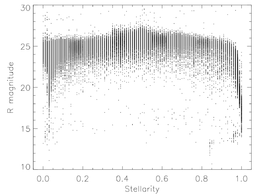
Figure 13.— SExtractor stellarity classification for objects in our catalog. The left panel shows stellarity versus total R-band AB magnitude and reflects confusion for saturated objects at $R<19$. The right panel shows a histogram of stellarity, with vertical solid lines separating galaxies ($stellarity\leq$0.3), uncertain objects (0.3$<stellarity<$0.8), and stars ($stellarity\geq$0.8). The classification is clean at $R<23$ (light histogram), shows an increasing fraction of uncertain objects at $23\leq R<25$ (medium histogram), and breaks down at $R\geq 25$ (dark histogram).

Figure 14 shows the locations of all objects in our catalog. There is an overabundance of objects along the image border which is not apparent to the eye but can be eliminated by removing the 574 objects with $flags\geq 8$, which identifies objects truncated by the image border. The one visual blemish is a line of spurious objects detected along a heavily saturated column extending from the brightest star in the field. This line is removed by eliminating all 1226 objects with $flags\geq 4$, which implies saturation in at least one filter.

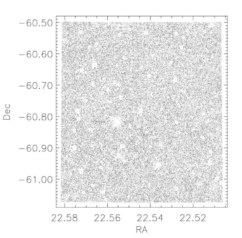
Figure 14.— Sky distribution of the 62968 objects in our photometric catalog (points) showing regions effectively masked out due to bright stars.

6. RESULTS

6.1. $R$-band number counts

The sky density of objects in our catalog is greatly reduced near the brightest stars, leading us to create a mask to properly exclude these regions from analyses of sky density and clustering. Our methodology is described in detail in L. Infante et al. (2005, in preparation). A careful analysis of the implied stellar and galaxy luminosity functions as a function of stellarity cut shows that stellar contamination is minimized with negligible loss of galaxy counts by requiring $stellarity<0.8$. The total $R$-band magnitude counts (from AUTO) are shown in Figure 15 and appear 90% complete to $R=24.5$ and 50% complete to $R=25.5$. Part of the incompleteness comes from AUTO beginning to underestimate the flux of very dim objects, as noted by Labbé et al. (2003). The fit for the number of galaxies per magnitude per square degree is $\log(N)=-3.52+0.34R$. Our slope of 0.34$\pm$0.01 agrees well with previous measurements of 0.321$\pm$0.001 by Smail et al. (1995), 0.361$\pm$0.004 by Capak et al. (2004), 0.31$\pm$0.01 and 0.34$\pm$0.01 in two different fields by Steidel & Hamilton (1993), and 0.39 by Tyson (1988). Our differential counts at $R=25.5$ of 1.3$\times 10^{5}$ agree well with the values of 1.2$\times 10^{5}$ reported by Steidel & Hamilton (1993).

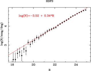
Figure 15.— $R$-band galaxy counts per unit magnitude per square degree with Poisson error bars and solid fit of $\log_{10}(N)=-3.52+0.34R$ based on counts at total AB magnitudes $20<R<24$. Incompleteness is minimal below total magnitude $R=24.5$ and reaches 50% around $R=25.5$.

6.2. $UVR$ Photometric Selection of Lyman Break Galaxies

Various filter sets have yielded success at finding LBGs, including $U_{n}G{\cal R}$ (Steidel et al., 1996b), SDSS $u^{\prime}g^{\prime}r^{\prime}i^{\prime}z^{\prime}$ (Bentz et al., 2004), $u^{\prime}BVRI$ (Cooke et al., 2005), $G{\cal R}i$ (Steidel et al., 1999), and $BRI$ (Gawiser et al. 2001, Prochaska et al. 2002). Figure 16 shows star colors expected and measured in our survey versus our adopted $UVR$ color selection criteria of

$$(U-V) > 1.2$$

$$-1.0 < (V-R)\;\;<\;0.6$$

$$(U-V) > 3.8(V-R)\;+\;1.2$$

$$19 < R\;\;\;<\;\;25.5\;\;\;,$$ (13)

where all magnitudes are AB. The color criteria shown as dashed lines in the figure result from the transformation of the $U_{n}$ $G$ ${\cal R}$ criteria described by Steidel et al. (1999) into $UVR$. Although the upper branch of the stellar distribution at red $V-R$ colors represents giants which are rare at our survey depth and high galactic latitude, we shifted our criteria to avoid this region as it also contains dim dwarf stars with correspondingly large errors in color, which are the primary expected source of interlopers. The region of the Steidel et al. criteria avoided by this shift had the highest fraction of interlopers and also shows a high interloper fraction in the more liberal $UVR$-selected subset of the Cooke et al. (2005) LBG sample. The LBG template curve falls within our selection region for $3.0<z<3.4$. At higher redshifts, the LBGs rapidly become too red in $V-R$ to distinguish from lower-redshift objects and are better selected as dropouts in $B-R$. We allow the color selection region to extend far to the blue in $V-R$ to account for the effect of Lyman $\alpha$ emission lines, which add flux in $V$.

Figure 16.— $U-V$ versus $V-R$ colors in our filter system (AB magnitudes) of a Lyman break galaxy template spectrum (Adelberger, priv. comm.) from redshift 0 to 3.4 (solid curve), the Pickles catalog of stars (plusses, Pickles, 1998), and the definite point sources in our catalog ($stellarity\geq 0.95$, points). The C and MC color selection regions used by Steidel et al. (2003) transformed into our UVR filter system are shown with dashed lines, and our adopted color selection region is shown with solid lines.

For spectroscopic selection and clustering analysis, objects with $U$ fluxes, $f_{U}$, less than their $1\sigma$ flux uncertainty, $\sigma_{U}$, were assigned an upper limit of $f_{U}=\sigma_{U}$ to make it less likely that negative sky fluctuations were responsible for turning a dim object in $U$ into a formal dropout in $U-V$. This correction avoids lower-redshift interlopers at the cost of some incompleteness. The vast majority of our LBG candidates are formal dropouts in the $U$ filter, with $f_{U}<\sigma_{U}$ before being set to these limit values. The limit values were used to generate the $U-V$ colors plotted in Fig. 17, which shows our full catalog including $z\simeq 3$ Lyman break galaxy candidates selected by their $UVR$ colors.

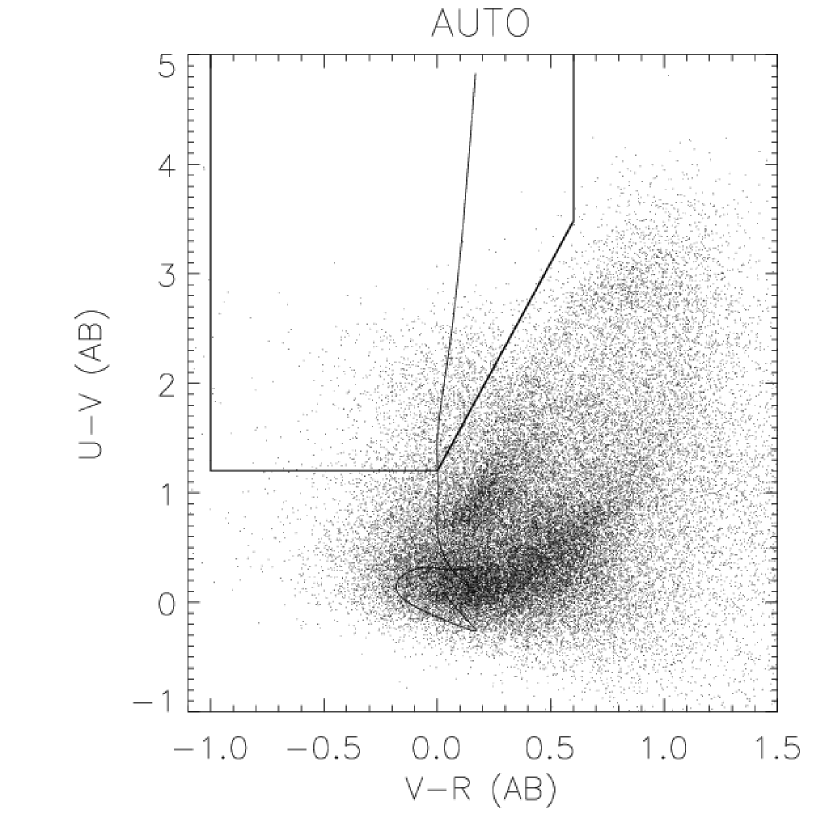
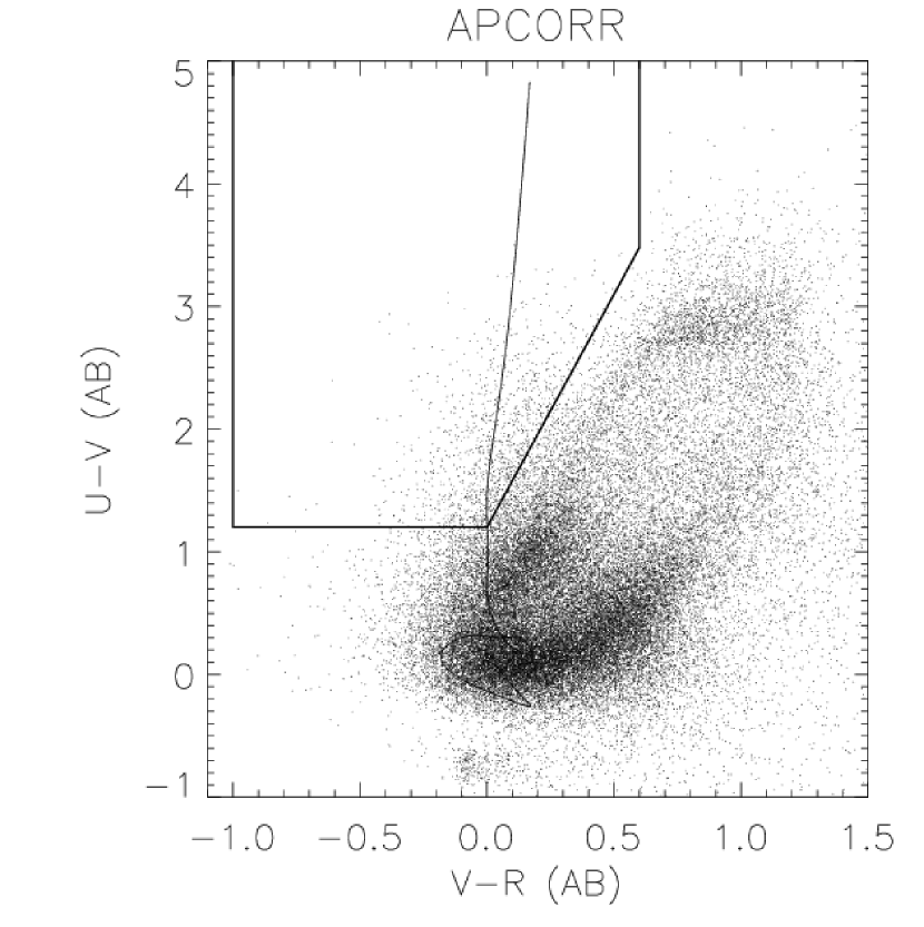
Figure 17.— $U-V$ versus $V-R$ colors of our full catalog (points) in AB magnitudes from SExtractor AUTO (Kron elliptical aperture) photometry (left panel) and from APCORR (corrected aperture) photometry (right panel). The LBG color selection region is shown with solid lines. The solid curve shows the colors of a Lyman break galaxy template spectrum over the interval $0<z<3.4$, with the interval $3.0<z<3.4$ falling in the selection region. The reduced scatter reflects improved performance of the APCORR fluxes, with a clearer definition of the main sequence and M dwarf locus.

Our selection criteria yield 1607 candidates in 1137 square arcminutes, or 1.4 arcmin^-2. Steidel et al. (1999) found 1.2 arcmin^-2 at ${\cal R}<25.5$ using stricter criteria than ours, Steidel et al. (2003) found 1.7 arcmin^-2 using the extended $U_{n}$ $G$ ${\cal R}$ criteria shown translated into $UVR$ in Figure 16, Capak et al. (2004) found 1.5 arcmin^-2 using UBR, and Cooke et al. (2005) found 1.5 arcmin^-2 using $u^{\prime}VRI$ criteria. Steidel et al. (2003) found a redshift distribution $<z>=2.96\pm 0.29$. Our $UVR$ criteria are expected to start selecting LBGs at redshifts higher by 0.16 because the red cutoff of the $U$-band filter and its effective wavelength after accounting for the MOSAIC II CCD QE are both $\sim 200$Å redder than for $U_{n}$. Our criteria are expected to stop selecting LBGs at redshifts higher by up to 0.4 because the Lyman alpha forest causes red $V-R$ colors at a higher redshift than in $G-{\cal R}$ due to the longer effective wavelength of $V$. Hence we expect $<z>=3.2\pm 0.4$, and this will be calibrated via spectroscopy.

Figure 18 shows the spatial distribution of these LBG candidates. We estimate the angular correlation function of these objects using the Landy & Szalay (1993) estimator

$$w(\theta)=\frac{DD-2DR+RR}{RR}\;\;\;,$$ (14)

where $DD$ represents the number of pairs at separation $\theta$ in the object catalog, $RR$ represents the appropriately-normalized number of pairs at separation $\theta$ in a Poisson-distributed mock catalog, and $DR$ represents the appropriately-normalized number of pairs at separation $\theta$ with one in the object catalog and the other in the mock catalog. This estimator has variance

$$var[w(\theta)]\simeq{\frac{(1+w(\theta))^{2}}{RR}}\;\;\;,$$ (15)

where the denominator gives the Poisson error contribution i.e. the number of pairs expected to be found in the bin centered on $\theta$ given the survey geometry and the total number of LBGs in the survey. The observed values of $w(\theta)$ must then be corrected for the integral constraint caused by estimating the true sky density of LBGs from our survey to find a power-law fit (Foucaud et al., 2003),

$$A_{w}\theta^{-\beta}=w_{obs}(\theta)+\frac{1}{\Omega^{2}}\int\int w(\theta)d\Omega_{1}d\Omega_{2}\;\;\;.$$ (16)

In practice, this correction is performed by using a modified estimator

$$w(\theta)=\frac{(1+A)DD-2DR+RR}{RR}\;\;\;,$$ (17)

where the correction factor $A$ is given by

$$A=\frac{\sum w(\theta)RR}{\sum RR}\;\;\;.$$ (18)

A is estimated iteratively and usually converges in a few iterations.

Figure 18.— Sky distribution of the 1607 LBG candidates in our catalog of E-HDFS showing some obvious clustering on small scales.

The angular correlation function found for Lyman break galaxy candidates in Figure 19 is $w(\theta)=(2.3\pm 1.0)\theta^{-0.8}$, where $\theta$ is measured in arcsec, intermediate between previous results for fixed $\beta=0.8$ from Giavalisco et al. (1998) of $A_{w}=1.4^{+1.5}_{-0.7}$ and Foucaud et al. (2003) of $A_{w}=5.2\pm 0.7$. This implies a correlation length for our sample of $r_{0}=5\pm 1$$h^{-1}_{70}$Mpc and an LBG bias factor of $b\simeq 2$ for the $\Lambda$CDM cosmology. These results will be updated after spectroscopic calibration of our $UVR$ LBG selection and by including our full square degree survey.

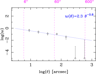
Figure 19.— Angular auto-correlation function of UVR-selected LBG candidates (open circles with error bars) with fit (solid line) labeled.

7. CONCLUSIONS

MUSYC is unique for its combination of depth and total area, for the coverage in X-ray, UV, mid- and far-infrared wavelengths and for providing the $UBVRIz^{\prime}$ plus near-infrared photometry needed to produce high-quality photometric redshifts over a square-degree of sky. This multiwavelength coverage will enable comparison of selection effects which have previously complicated the study of galaxies in the high-redshift universe. The large area ensures good statistics for studies of clustering, luminosity functions, and surface densities.

We expect that the careful attention paid to optimized photometry methods and the estimation of accurate photometric uncertainties will allow our public data to make a significant impact for a wide range of scientific studies. In particular, this high-quality $UBVRIz^{\prime}$ data, combined with forthcoming near-infrared photometry, should yield photometric redshifts with good accuracy. It is interesting to note that some of the standard techniques perform well despite making a number of idealized assumptions. For instance, we found that the optimal point source apertures are remarkably close in diameter to the idealized case of 1.35 fwhm due to a partial cancellation of the non-Gaussian PSF preferring a larger aperture and the correlated noise preferring a smaller aperture. The more traditional approach of using $2^{\prime\prime}$ apertures produces biases in point-source colors. Alleviating those biases by “PSF-matching” i.e. smoothing the images to match the fwhm of the image with the worst seeing must be done carefully given the non-Gaussian PSF shapes and will result in degraded signal-to-noise for point sources. Estimates of point source detection depth that assume uncorrelated noise and extrapolate from the rms pixel noise will overestimate the depth by about 0.5 magnitudes for 2^′′ or 3^′′ apertures.

The APCORR fluxes introduced in this paper perform extremely well, as seen in Fig. 17. The nearly unbiased performance of APCORR fluxes for both point sources and extended objects is impressive, and the correlated errors between filters for extended objects are acceptable if the flux is misestimated by a constant fraction in all filters. However, one should use caution when calculating photometric redshifts on extended objects in photometric catalogs generated using apertures which might miss a different fraction of the object flux in each filter. The best results should be obtained by using the APCORR fluxes in our catalog for unresolved and barely resolved sources, with further investigation needed to determine whether APCORR outperforms AUTO for extended sources.

Our $UBVRIz^{\prime}$ images and catalogs of the $33^{\prime}\times 34.5^{\prime}$ Extended Hubble Deep Field South are available to the public at http://www.astro.yale.edu/MUSYC .

Appendix A Optimal Weights for Image Stacking for Point Sources and Extended Sources

We wish to combine a series of processed individual images which have signal $S_{i}$ and noise $N_{i}$. The exact signal obviously depends on which star is measured, but if a common set of stars are considered the variations in signal will be due to differences in exposure time, cirrus extinction, and atmospheric extinction. The noise should be sky-dominated away from bright objects but measuring the rms in “blank” regions of sky properly accounts for the readnoise as well. For surface-brightness-optimization we want to average the total signal from a set of stars, as measured by the IRAF routine phot or the inverse of the mscscale header output by mscimatch. For point-source-optimization we want to determine the average signal that falls within our eventual optimal aperture, which will have a diameter of roughly 1.35 times the fwhm of the final image. The seeing in the final image can be estimated or measured from an initially unweighted stack, or an iterative procedure can be used. Alternatively, a correction to the total star counts $S^{tot}_{i}$ can be calculated by integrating an assumed Gaussian PSF out to the diameter of the expected optimal aperture of radius R; if the seeing in each image is $\sigma_{i}=$ fwhm${}_{i}/2.35$, we obtain

$$S_{i}=S^{tot}_{i}[1-\exp(-R^{2}/2\sigma_{i}^{2})]\;\;\;.$$ (A1)

In either type of optimization, the noise value used should be the background rms for the expected aperture size, which depends on the level of noise correlation between pixels. Assuming that the noise correlations have the same behavior in each individual image, it is sufficient to use the pixel-by-pixel rms i.e. $\sigma_{1}$ measured in each image since this will produce the right relative weights.

One can derive the weights that optimize the $S/N$ of the combined image by noting that the combined image will have $S=\sum_{i}w_{i}S_{i}$ and $N^{2}=\sum_{i}w_{i}^{2}N_{i}^{2}$ (the weighted sum is just an unweighted sum of new images having signal $w_{i}S_{i}$ and noise $w_{i}N_{i}$). Maximizing the function $S/N$ produces the result $w_{i}=kS_{i}/N_{i}^{2}$, where multiplying all the weights by a constant $k$ preserves the final $S/N$. In astronomy, it is typical to first scale the images to have equal signal levels; this accounts for differences in exposure time and extinction to provide constant photometry and makes it easier to delete outlying pixels due to cosmic rays, satellite trails, etc. The IRAF-mscred routine mscstack performs this scaling by multiplying by the mscscale header value and then uses a weightfile to weight the scaled images. So the weights used must be for the scaled images, which leads to the formula for surface-brightness-optimized weighting of

$$w_{i}^{SB}=\frac{1}{(mscscale_{i}\times rms_{i})^{2}}\;\;\;,$$ (A2)

which is equivalent to $(S_{i}/N_{i})^{2}$ in the original image because the image being weighted is different than the one for which $S_{i}$ and $N_{i}$ were measured. The output image is the same since instead of multiplying $S_{i}$ by $S_{i}/N_{i}^{2}$ and adding we are equating the signal levels and then multiplying 1 by $(S_{i}/N_{i})^{2}$, but performing the scaling first makes it easier to remove outlying pixels from this sum as mentioned above. The weights being used correspond to $S/N^{2}$ for the scaled images; they reduce to the familiar case of inverse-variance weighting since the signal levels have already been equalized. For point-source optimized weighting we use

$$w_{i}^{PS}=\left(\frac{factor_{i}}{mscscale_{i}\times rms_{i}}\right)^{2}\;\;\;,$$ (A3)

where $factor_{i}$ is given by

$$factor_{i}=1-\exp\left(-1.3\frac{fwhm_{stack}^{2}}{fwhm_{i}^{2}}\right)\;\;\;,$$ (A4)

where we have re-expressed the formula for $S_{i}$ from Eq. A1 in terms of the measured seeing in an unweighted (or surface-brightness optimized) stack, $fwhm_{stack}$, and that in each individual image $fwhm_{i}$. Again, these weights are only valid when used on the post-scaled images, and they differ by a factor of $S_{i}$ from the weights appropriate for the original images.

Due to the large number of individual exposures taken in e.g. $U$-band and multiple observing runs, it is sometimes necessary to perform stacking as an iterative procedure. To do this, the signal, noise, and seeing in the intermediate stacked images should be measured empirically as before. Then mscstack or the equivalent can be used to stack these intermediate images just as if they were individual images, scaling by the new mscscale values and calculating a new weights file using the above equations. As long as the final seeing is estimated well, no loss of signal-to-noise should occur from the iteration.

A corollary question is when to discard an image with poor $S/N$ rather than to include it in the stack. The formal answer appears to be never as $w_{i}>0$ for all $i$. The magic of the optimal weighting formula can be seen:

$$\frac{S}{N}=\frac{\sum_{i}w_{i}S_{i}}{\sqrt{\sum_{i}w_{i}^{2}N_{i}^{2}}}=\frac{\sum_{i}S_{i}^{2}/N_{i}^{2}}{\sqrt{\sum_{i}S_{i}^{2}/N_{i}^{2}}}=\sqrt{\sum_{i}S_{i}^{2}/N_{i}^{2}}\;\;\;.$$ (A5)

Hence the optimal weights cause $S/N$ to add in quadrature so it will never formally decrease no matter how poor an input image is. Note that having a magnitude of extinction or twice the seeing still leaves an image with significant $S/N$; a $S/N$ threshold of 40% would require discarding images with about 2 times worse seeing or 1 magnitude of extinction (if the sky background is unaffected). The $S/N$ of the combination of the image with a given $S/N$ and an image with 40% of that $S/N$ is 8% higher than that of the better image alone so this is somewhat useful. A conservative approach would be to cut entirely any images with $S/N<10$% that of the median image as a way of reducing systematic effects not accounted for by these idealized formulae.

Appendix B Optimal Weights for Point Source Detection

Irwin (1985) showed using simulations that the best performance for point source detection was achieved by filtering the image with the PSF itself. This result is derived in the SExtractor manual using Fourier transforms. In practice due to the constraints of computation time one chooses to cut off the PSF at a finite radius, as is standard in the convolution kernels offered as part of the SExtractor package. The general case for an optimized weighted sum of pixel values $S=\sum_{j}w_{j}S_{j}$, where each pixel has signal $S_{j}$ and noise $N_{j}$, can be derived in analogy to the result for adding images found above, yielding $w_{j}\propto S_{j}/N_{j}^{2}$. The constant background noise for sky-dominated objects thus leads to a filter of the precise shape of the PSF. For objects significantly brighter than the sky, $S=N^{2}$ giving constant weight i.e. a tophat which gradually morphs into the roughly Gaussian shape of the PSF as you move far enough away from the object center for the sky to dominate the noise. SExtractor only allows for a fixed convolution kernel so we optimized the detection for sky-dominated objects by using the PSF (truncated to 7$\times$7 pixels) as our filter.

By the same argument, the optimum signal-to-noise measurement of the photometry of a point source will be obtained by a weighted sum of pixel fluxes weighted using the PSF shape itself centered at the barycenter of the object. This is typically referred to as “PSF photometry” but it is not a supported feature of SExtractor photometry, just of object detection. Note that this is no longer strictly optimal when the noise is correlated between pixels as we have found in our images, since the derivation of the optimal weights for each pixel assumed uncorrelated noise. We decided against using PSF photometry for this reason, and also because many of our science objects are slightly resolved and this would overweight the fluxes in their core, increase the risk of color biases, and complicate the task of correcting the aperture fluxes of extended objects.

Table 1MUSYC Fields

Field	RA	Dec	Galactic	Ecliptic	E(B-V)	100$\mu$m Em.	N(HI)
			Coords. (deg)	Coords. (deg)		(MJy/sr)	(cm-2)
E-HDFS	22:32:35.6	-60:47:12	(328,-49)	(311,-47)	0.03	1.37	1.6E+20
E-CDFS	03:32:29.0	-27:48:47	(224,-54)	(41,-45)	0.01	0.40	9.0E+19
SDSS1030+05	10:30:27.1	05:24:55	(239,50)	(157,-4)	0.02	1.01	2.3E+20
CW1255+01	12:55:40	01:07:00	(306,64)	(192,7)	0.02	0.81	1.6E+20

Table 2Optical Observations of E-HDFS with CTIO4m+MOSAIC-II

Dates	Filter	Number of	Exposure	Seeing
		Exposures	Time (s)	(′′)
2002 Oct 6,8	$U$	47	28200	1.40
2002 Oct 6,8,10	$B$	13	7500	1.35
2002 Oct 6,10,12	$V$	30	10440	0.90
2002 Oct 6,10,12	$R$	21	6300	0.85
2002 Oct 6,12	$I$	26	6300	0.85
2002 Oct 6,12	$z^{\prime}$	11	2700	0.90
2003 May 26,27	$U$	25	15000	1.20
2003 May 27	$B$	10	6000	1.10
2003 May 27,28	$R$	20	6000	1.10
2003 May 26	$z^{\prime}$	15	3600	1.30

Table 3Results of photometric calibration for 2002 October 6 in AB magnitudes

Filter	Airmass	Seeing	Zeropoint	Airmass coeff.	Color term
		(′′)
U	1.34	2.1	24.15$\pm$0.012	0.55	(-0.08$\pm$0.01)$\times(U-B)_{\mathrm{AB}}$
B	1.38	1.8	25.24$\pm$0.009	0.24	(-0.03$\pm$0.004)$\times(U-V)_{\mathrm{AB}}$
V	1.40	1.6	25.64$\pm$0.004	0.15	(0.03$\pm$0.003)$\times(B-R)_{\mathrm{AB}}$
R	1.42	1.5	25.95$\pm$0.005	0.09	(-0.009$\pm$0.005)$\times(V-I)_{\mathrm{AB}}$
I	1.44	1.5	25.40$\pm$0.006	0.05	(0.006$\pm$0.017)$\times(R-I)_{\mathrm{AB}}$
$z^{\prime}$	1.46	1.5	24.61$\pm$0.014	0.03	(-0.06$\pm$0.054)$\times(R-I)_{\mathrm{AB}}$

Table 4Total Exposure Time and Photometric Zeropoints for E-HDFS Images

Filter	Exposure	Mag. Zeropoint	Flux Zeropoint
	Time (s)	(AB mag @ 1 count s-1)	($\mu$Jy (count/s)-1)
$BVR$	35340	24.29	0.698
U	42600	23.35	1.660
B	13200	24.85	0.417
V	10440	25.40	0.251
R	11700	25.75	0.182
I	6000	25.27	0.283
$z^{\prime}$	6000	24.39	0.637

Table 5Fit parameters for background fluctuations in counts $s^{-1}$ as a function of aperture size using Eq. 4

Filter	$\sigma_{1}$	$\alpha$	$\beta$
BVR	0.0029	0.68	1.47
U	0.0012	0.82	1.30
B	0.0043	0.88	1.33
V	0.014	0.69	1.34
R	0.019	0.69	1.40
I	0.032	0.72	1.42
$z^{\prime}$	0.030	0.87	1.41

Table 6Seeing, Apertures, and Source Detection Limits for E-HDFS Images

Filter	IRAF fwhm	SE fwhm	SE $r_{1/2}$	Optimal Aperture	Flux Enclosed	Source Detection
	Mode (′′)	Median (′′)	Median (′′)	(′′)	(Fractional)	Limit (5 $\sigma$, AB)
BVR	0.95	0.99	0.59	1.2	0.48	26.3
U	1.30	1.48	0.78	1.6	0.50	26.0
B	1.25	1.29	0.71	1.4	0.47	26.1
V	0.90	0.96	0.56	1.2	0.52	26.0
R	0.90	0.97	0.58	1.2	0.49	25.8
I	0.80	0.99	0.56	1.2	0.49	24.7
$z^{\prime}$	0.90	1.06	0.62	1.2	0.43	23.6

Table 7Optical source catalog: astrometric and photometric parameters determined from $BVR$ detection image and $UBVRIz^{\prime}$ photometry.

Number	Name	RA	Dec	x	y	Stellarity	r1/2	A_IMAGE
	MUSYC-	(hrs)	(deg)				(′′)	(′′)
B_IMAGE	$\theta$_IMAGE	FLAGS	$f$_auto_U	$\sigma$_auto_U	$f$_auto_B	$\sigma$_auto_B	$f$_auto_V	$\sigma$_auto_V
(′′)	ccw from X-axis		($\mu$Jy)	($\mu$Jy)	($\mu$Jy)	($\mu$Jy)	($\mu$Jy)	($\mu$Jy)
$f$_auto_R	$\sigma$_auto_R	$f$_auto_I	$\sigma$_auto_I	$f$_auto_$z^{\prime}$	$\sigma$_auto_$z^{\prime}$	$f$_apcorr_U	$\sigma$_apcorr_U	$f$_apcorr_B
($\mu$Jy)	($\mu$Jy)	($\mu$Jy)	($\mu$Jy)	($\mu$Jy)	($\mu$Jy)	($\mu$Jy)	($\mu$Jy)	($\mu$Jy)
$\sigma$_apcorr_B	$f$_apcorr_V	$\sigma$_apcorr_V	$f$_apcorr_R	$\sigma$_apcorr_R	$f$_apcorr_I	$\sigma$_apcorr_I	$f$_apcorr_$z^{\prime}$	$\sigma$_apcorr_$z^{\prime}$
($\mu$Jy)	($\mu$Jy)	($\mu$Jy)	($\mu$Jy)	($\mu$Jy)	($\mu$Jy)	($\mu$Jy)	($\mu$Jy)	($\mu$Jy)
0	J223023.68-604817.4	22.506580	-60.804850	7397.04	3613.83	0.490000	0.377004	0.0771630
0.0771630	45.0000	16	0.00599998	0.0123559	0.0268263	0.0133826	0.0721889	0.0189753
0.0535715	0.0192685	0.0584936	0.0536170	0.105203	0.142492	0.0153194	0.0299205	0.0582284
0.0300672	0.129481	0.0322477	0.0994542	0.0346933	0.0963358	0.0964758	0.129852	0.292286
1	J223024.28-604008.9	22.506747	-60.669150	7395.69	5443.56	0.380000	0.381543	0.0771630
0.0771630	45.0000	16	0.0545032	0.0134836	0.0528900	0.0133148	0.0600472	0.0181627
0.0531777	0.0189421	0.0346594	0.0537312	-0.0605122	0.0999073	0.123143	0.0319542	0.111140
0.0292123	0.0983857	0.0301251	0.0985063	0.0331430	0.0733320	0.0938256	-0.113113	0.287106
2	J223023.85-604558.3	22.506627	-60.766210	7397.14	4134.88	0.490000	0.555360	0.216003
0.133500	-0.200000	24	0.0909909	0.0243018	0.0549541	0.0255182	0.0440691	0.0353969
0.130563	0.0386372	0.159939	0.108677	0.0605380	0.286208	0.100151	0.0285476	0.0699377
0.0270144	0.0861040	0.0280836	0.125653	0.0311628	0.113170	0.0863858	0.0282574	0.261025
3	J223024.98-603027.9	22.506940	-60.507770	7394.68	7619.57	0.940000	0.328410	0.199716
0.120951	18.8000	24	-0.0217973	0.0159112	0.000543353	0.0123818	0.115021	0.0169463
300.840	0.0511371	577.641	0.128364	-0.00643368	0.124763	-0.0458961	0.0422158	-0.000965204
0.0289711	0.222445	0.0300914	601.662	0.125434	1191.94	0.301193	0.00430643	0.280111
4	J223023.35-605242.2	22.506487	-60.878400	7397.96	2622.20	0.610000	0.613032	0.369528
0.202653	-5.40000	24	-0.00917560	0.0288420	0.0469781	0.0383380	0.134234	0.0542395
0.155328	0.0622344	-0.104166	0.130648	0.110060	0.458585	-0.0224367	0.0274903	0.100572
0.0275703	0.155969	0.0290837	0.143652	0.0332477	0.0475046	0.0869854	0.677608	0.276257

Note. — This table is published in its entirety in the electronic edition of the Astrophysical Journal. A portion is shown here for guidance regarding its form and content. Due to geometry, these first few objects are near the image border and have poor photometry, leading to their large FLAG values.

References

- Abazajian et al. (2005) Abazajian, K. et al. 2005, AJ, 129, 1755
- Altmann et al. (2004) Altmann, M., Méndez, R. A., Ruiz, M. T., van Altena, W., Gawiser, E., & van Dokkum, P. 2004, in 14th European Workshop on White Dwarfs, ASP Conference Series, ed. D. Koester & S. Moehler, Vol. 999
- Arnouts et al. (2001) Arnouts, S. et al. 2001, A&A, 379, 740
- Bechtold et al. (2003) Bechtold, J. et al. 2003, ApJ, 588, 119
- Bentz et al. (2004) Bentz, M. C., Osmer, P. S., & Weinberg, D. H. 2004, ApJ, 600, L19
- Bertin & Arnouts (1996) Bertin, E. & Arnouts, S. 1996, A&AS, 117, 393
- Burstein & Heiles (1978) Burstein, D. & Heiles, C. 1978, ApJ, 225, 40
- Capak et al. (2004) Capak, P. et al. 2004, AJ, 127, 180
- Chen et al. (2002) Chen, H. et al. 2002, ApJ, 570, 54
- Cooke et al. (2005) Cooke, J., Wolfe, A. M., Prochaska, J. X., & Gawiser, E. 2005, ApJ, 621, 596
- Daddi et al. (2004) Daddi, E., Cimatti, A., Renzini, A., Vernet, J., Conselice, C., Pozzetti, L., Mignoli, M., Tozzi, P., Broadhurst, T., di Serego Alighieri, S., Fontana, A., Nonino, M., Rosati, P., & Zamorani, G. 2004, ApJ, 600, L127
- Davis et al. (2003) Davis, M. et al. 2003, in Discoveries and Research Prospects from 6- to 10-Meter-Class Telescopes II. Edited by Guhathakurta, Puragra. Proceedings of the SPIE, Volume 4834, 161
- Dickinson et al. (2004) Dickinson, M. et al. 2004, ApJ, 600, L99
- Farrah et al. (2004) Farrah, D., Priddey, R., Wilman, R., Haehnelt, M., & McMahon, R. 2004, ApJ, 611, L13
- Foucaud et al. (2003) Foucaud, S., McCracken, H. J., Le Fèvre, O., Arnouts, S., Brodwin, M., Lilly, S. J., Crampton, D., & Mellier, Y. 2003, A&A, 409, 835
- Franx et al. (2003) Franx, M. et al. 2003, ApJ, 587, L79
- Fukugita et al. (1996) Fukugita, M., Ichikawa, T., Gunn, J. E., Doi, M., Shimasaku, K., & Schneider, D. P. 1996, AJ, 111, 1748
- Gawiser et al. (2001) Gawiser, E., Wolfe, A. M., Prochaska, J. X., Lanzetta, K. M., Yahata, N., & Quirrenbach, A. 2001, ApJ, 562, 628
- Giacconi et al. (2002) Giacconi, R. et al. 2002, ApJS, 139, 369
- Giavalisco et al. (1998) Giavalisco, M., Steidel, C. C., Adelberger, K. L., Dickinson, M. E., Pettini, M., & Kellogg, M. 1998, ApJ, 503, 543
- Giavalisco et al. (2004) Giavalisco, M. et al. 2004, ApJ, 600, L93
- Irwin (1985) Irwin, M. J. 1985, MNRAS, 214, 575
- Jannuzi & Dey (1999) Jannuzi, B. T. & Dey, A. 1999, in Astronomical Society of the Pacific Conference Series, 111
- Labbé et al. (2003) Labbé, I. et al. 2003, AJ, 125, 1107
- Lacy et al. (2004) Lacy, M. et al. 2004, ApJS, 154, 166
- Landolt (1992) Landolt, A. U. 1992, AJ, 104, 340
- Landy & Szalay (1993) Landy, S. D. & Szalay, A. S. 1993, ApJ, 412, 64
- Le Fèvre et al. (2004) Le Fèvre, O. et al. 2004, A&A, 417, 839
- Lira et al. (2004) Lira, P. et al. 2004, ArXiv Astrophysics e-prints, astro-ph/0407396
- MacDonald et al. (2004) MacDonald, E. C., Allen, P., Dalton, G., Moustakas, L. A., Heymans, C., Edmondson, E., Blake, C., Clewley, L., Hammell, M. C., Olding, E., Miller, L., Rawlings, S., Wall, J., Wegner, G., & Wolf, C. 2004, MNRAS, 352, 1255
- Palunas et al. (2000) Palunas, P. et al. 2000, ApJ, 541, 61
- Pickles (1998) Pickles, A. J. 1998, PASP, 110, 863
- Prochaska et al. (2002) Prochaska, J. X., Gawiser, E., Wolfe, A. M., Quirrenbach, A., Lanzetta, K. M., Chen, H., Cooke, J., & Yahata, N. 2002, AJ, 123, 2206
- Radovich et al. (2004) Radovich, M. et al. 2004, A&A, 417, 51
- Rix et al. (2004) Rix, H. et al. 2004, ApJS, 152, 163
- Rosati et al. (2002) Rosati, P. et al. 2002, ApJ, 566, 667
- Schlegel et al. (1998) Schlegel, D. J., Finkbeiner, D. P., & Davis, M. 1998, ApJ, 500, 525
- Smail et al. (1995) Smail, I., Hogg, D. W., Yan, L., & Cohen, J. 1995, ApJ, 449, L105
- Smith et al. (2002) Smith, J. A. et al. 2002, AJ, 123, 2121
- Steidel et al. (1999) Steidel, C. C., Adelberger, K. L., Giavalisco, M., Dickinson, M., & Pettini, M. 1999, ApJ, 519, 1
- Steidel et al. (2003) Steidel, C. C., Adelberger, K. L., Shapley, A. E., Pettini, M., Dickinson, M., & Giavalisco, M. 2003, ApJ, 592, 728
- Steidel et al. (1996a) Steidel, C. C., Giavalisco, M., Dickinson, M., & Adelberger, K. L. 1996a, AJ, 112, 352
- Steidel et al. (1996b) Steidel, C. C., Giavalisco, M., Pettini, M., Dickinson, M., & Adelberger, K. L. 1996b, ApJ, 462, L17
- Steidel & Hamilton (1993) Steidel, C. C. & Hamilton, D. 1993, AJ, 105, 2017
- Steidel et al. (2002) Steidel, C. C., Hunt, M. P., Shapley, A. E., Adelberger, K. L., Pettini, M., Dickinson, M., & Giavalisco, M. 2002, ApJ, 576, 653
- Szalay et al. (1999) Szalay, A. S., Connolly, A. J., & Szokoly, G. P. 1999, AJ, 117, 68
- Teplitz et al. (2001) Teplitz, H. I., Hill, R. S., Malumuth, E. M., Collins, N. R., Gardner, J. P., Palunas, P., & Woodgate, B. E. 2001, ApJ, 548, 127
- Treister et al. (2004) Treister, E. et al. 2004, ApJ, 616, 123
- Tyson (1988) Tyson, J. A. 1988, AJ, 96, 1
- van Dokkum et al. (2003) van Dokkum, P. G. et al. 2003, ApJ, 587, L83
- van Dokkum et al. (2004) —. 2004, ApJ, 611, 703
- Williams et al. (1996) Williams, R. E. et al. 1996, AJ, 112, 1335
- Williams et al. (2000) —. 2000, AJ, 120, 2735
- Wolf et al. (2001) Wolf, C., Dye, S., Kleinheinrich, M., Meisenheimer, K., Rix, H.-W., & Wisotzki, L. 2001, A&A, 377, 442
- Wolf et al. (2004) Wolf, C. et al. 2004, A&A, 421, 913
- Wolfe et al. (2005) Wolfe, A. M., Gawiser, E., & Prochaska, J. X. 2005, ARA&A, 43, 861
- Wolfe et al. (1986) Wolfe, A. M., Turnshek, D. A., Smith, H. E., & Cohen, R. D. 1986, ApJS, 61, 249
- York et al. (2000) York, D. G. et al. 2000, AJ, 120, 1579