Scalings between Physical and their Observationally Related Quantities of Merger Remnants

Se presentan relaciones de escala entre la velocidad virial ($V$) y la dispersión de velocidades uni-dimensional central ($\sigma_{0}$); el radio gravitacional ($R_{\rm v}$) y el radio efectivo ($R_{\rm e}$); y la masa total ($M$) y la masa luminosa ($M_{\rm L}$) encontradas en simulaciones de $N$-cuerpos de fusiones binarias entre galaxias espirales. Estas relaciones son de la forma $V^{2}\propto\sigma_{0}^{\alpha}$, $R_{\rm v}\propto R_{\rm e}^{\beta}$ y $M\propto M_{\rm L}^{\gamma}$. Los valores particulares obtenidos para $\{\alpha,\beta,\gamma\}$ dependen del método de ajuste utilizado [mínimos cuadrados ordinarios (ols) o regresión ortogonal de distancia (odr)], el tipo de perfil supuesto [de Vaucouleurs (deV) or Sérsic (S)], y el tamaño del intervalo radial donde se hace el ajuste. Los índices $\alpha$ y $\gamma$ resultan ser los más sensibles al procedimiento de ajuste, obteniéndose para el ols un promedio $\langle\alpha\rangle_{\rm ols}=1.51$ y $\langle\gamma\rangle_{\rm ols}=0.69$, mientras que para el odr un $\langle\alpha\rangle_{\rm odr}=2.35$ y $\langle\gamma\rangle_{\rm odr}=0.76$. El índice $\beta$ depende más de el perfil adoptado, con $\langle\beta\rangle_{\rm{deV}}=0.13$ y $\langle\beta\rangle_{\rm{S}}=0.27$. Concluímos que los remanentes de fusiones formados de manera no disipativa tienen un rompimiento fuerte de homología estructural y cinemática.

Abstract

We present scaling relations between the virial velocity ($V$) and the one-dimensional central velocity dispersion ($\sigma_{0}$); the gravitational radius ($R_{\rm v}$) and the effective radius ($R_{\rm e}$); and the total mass ($M$) and the luminous mass ($M_{\rm L}$) found in $N$-body simulations of binary mergers of spiral galaxies. These scalings are of the form $V^{2}\propto\sigma_{0}^{\alpha}$, $R_{\rm v}\propto R_{\rm e}^{\beta}$ and $M\propto M_{\rm L}^{\gamma}$. The particlar values obtained for $\{\alpha,\beta,\gamma\}$ depend on the method of fitting used [ordinary least-squares (ols) or orthogonal distance regression (odr)], the assumed profile [de Vaucouleurs (deV) or Sérsic (S)], and the size of the radial interval where the fit is done. The $\alpha$ and $\gamma$ indexes turn out more sensitive to the fitting procedure, obtaining for the ols a mean $\langle\alpha\rangle_{\rm ols}=1.51$ and $\langle\gamma\rangle_{\rm ols}=0.69$, while for the odr $\langle\alpha\rangle_{\rm odr}=2.35$ and $\langle\gamma\rangle_{\rm odr}=0.76$. The $\beta$ index depends more on the adopted type of profile, with $\langle\beta\rangle_{\rm{deV}}=0.13$ and $\langle\beta\rangle_{\rm{S}}=0.27$. We conclude that dissipationless formed remnants of mergers have a strong breaking of structural and kinematical homology.

0.1 Introduction

Toomre’s (1977) idea that the merging of spirals could lead to an elliptical galaxy has found ground evidence, both theoretical and observational (e.g., Barnes 1998, Schweizer 1998), although some questions remain open (e.g., Peebles 2002, Chiosi & Carraro 2002).

Ellipticals show a number of regularities among their kinematical and structural properties that have been recognized in the past, such as the Kormendy and Faber-Jackson relation, and the Fundamental Plane of Ellipticals (e.g., Kormendy 1977, Faber & Jackson 1976, Bernardi et al. 2003a,b).

Understanding the physical origin of these relations is important since they are intimately related to their formation and evolutionary history. Obtaining theoretical scalings relations among physical and observational quantities depends on our knowledge, for example, of the star formation process, the distribution of dark matter in ellipticals, and the kinematics of remnants of spiral mergers. Given the complexities of the problem, we restrict ourselves here to obtain scaling relations resulting solely from dissipationless simulations of mergers of spirals.

In a related paper (Aceves & Velázquez 2005) the accumulated effects of spatial and kinematical homology breaking on the determination of a Fundamental Plane (FP) like relation for remnants was studied, but no detailed examination of how the different physical quantities involved scaled with their observational counterparts. In this work we address this matter in more detail, and include two more merger simulations than in Aceves & Velázquez (2005).

In particular, we consider here only quantities involved in the virial theorem and we determine their dependences with their observational counterparts:

$$V^{2}\propto\sigma_{0}^{\alpha},\quad R_{\rm g}\propto R_{\rm e}^{\beta},\quad M\propto M_{\rm L}^{\gamma}\,;$$ (1)

where $V$ is virial velocity, $\sigma_{0}$ the one-dimensional central velocity dispersion, $R_{\rm g}$ the gravitational radius, $R_{\rm e}$ the effective radius (i.e., that enclosing half of the luminous matter), $M$ the total mass of the system, and $M_{\rm L}$ the luminous mass. Homology between the physical and observational quantities requires that $\alpha=2$, and $\beta=\gamma=1$ in expression (1).

A further motivation for this study stems from the fact that behavior of the previous relations bears direct impact on the estimate of a dynamical mass $M_{\rm dyn}$ in ellipticals (e. g., Padmanabhan et al. 2004). It is common to assume in such studies an homologous relation of the form $M_{\rm dyn}\propto\sigma_{0}^{2}R_{\rm e}$. However, as we will see, merger remnants show an important deviation from homology that most probably reflect the actual situation in ellipticals. Thus this effect of non-homology would need to be taken into consideration when estimating the dynamical mass of ellipticals. However, the study of such a a problem is out of the scope of the present work.

This paper has been organized as follows. In Section 2, we summarize the numerical models of spiral galaxies used. We describe the initial conditions for the encounters as well as we provide some information on the computational aspects on the simulations carried out. In Section 3 we present the method used to determine the physical quantities $\{V,R_{\rm g},M\}$ and their observationally related ones $\{\sigma_{0},R_{\rm e},M_{\rm L}\}$. Also, the fitting procedures used to obtain the scaling indexes in (1) are indicated. In Section 4, the results obtained for $\{\alpha,\beta,\gamma\}$ in (1) are presented. Finally, in Section 5, we summarize our main conclusions.

0.2 Galaxy models and initial conditions for encounters

0.2.1 Galaxy Models

Our spiral galaxy models consist of a spherical dark halo and a stellar disk component. The contribution of a central bulge is not considered here. The disk profile has the functional form

$$\rho_{\rm d}(R,z)=\frac{M_{\rm d}}{4\pi R^{2}_{\rm d}z_{d}}\exp(-R/R_{\rm d})\,{\rm sech}^{2}(z/z_{d})\;,$$ (2)

where $R_{\rm d}$ and $z_{\rm d}$ are the radial and vertical scale-lengths of the disk, respectively. The vertical length, $z_{\rm d}$, is randomly taken from the interval $(0.1-0.2)R_{\rm d}$; where $R_{\rm d}$ is obtained as indicated below.

The dark halo follows a Navarro, Frenk & White (NFW, 1997) profile, modified with an exponential cutoff:

$$\rho_{\rm h}(r)=\frac{M_{\rm h}\,\alpha_{\rm h}}{4\pi r(r+r_{\rm s})^{2}}\ \exp\left[-\left(\frac{r}{r_{200}}+q\right)^{2}\right]\;,$$ (3)

with

$$\alpha_{\rm h}=\frac{\exp(q^{2})}{\sqrt{\pi}q\exp(q^{2}){\rm Erfc}(q)+\frac{1}{2}\exp(q^{2}){\rm E}_{1}(q^{2})-1};$$

where ${\rm Erfc}(x)$ is the complimentary error function and ${\rm E}_{1}(x)$ the exponential integral. The scale radius of the dark matter profile is $r_{\rm s}$, $c=1/q=r_{200}/r_{\rm s}$ is the concentration, and $M_{\rm h}$ is the halo mass; $r_{200}$ is defined as the radius where the mean interior density is 200 times the critical density.

The properties of the disk are set up satisfying the Tully-Fisher relation (Tully & Fisher 1977, Giovanelly et al. 1997). This is carried out by following the study of Shen, Mo & Shu (2002, hereafter SMS) and using the disk galaxy formation model of Mo, Mao & White (1998, hereafter MMW); from which we can obtain $R_{\rm d}$.

In the MMW framework five parameters are required to obtain the radial scale-length of the disk. These are the circular velocity $V_{\rm c}$ at $r_{200}$, the dimensionless spin parameter $\lambda$, the concentration $c$ of the dark halo, the fraction of disk to halo mass $m_{\rm d}$, the fraction of angular momentum in the disk to that in the halo $j_{\rm d}$. We have followed the procedure outlined by SMS to construct our galaxy models, and chosen an epoch for the formation of disks at a redshift of $z=1$ (Peebles 1993).

We have selected only spirals with circular velocities in the range from 50 to 300 km s^-1, and with a disk stability parameter $\varepsilon_{\rm m}$$\,\geq\,$$0.9$; where $\varepsilon_{\rm m}$=$V_{\rm m}(GM_{\rm d}/R_{\rm d})^{-1/2}$ and $V_{\rm m}$ is the maximum rotation velocity (Efsthatiou, Lake & Negroponte 1982, Syer, Mao & Mo 1997). From an ensemble of random points constructed according to the scheme of SMS, and satisfying the previous conditions, we obtained the final properties of the 24 galaxies that take part in our 12 binary merger simulations.

In Table 1 the particular values for each galaxy model constructed are listed; where $N_{\rm h}$ and $N_{\rm d}$ are the number of particles used in the halo and disk, respectively. The last column lists the pericenter radius $R_{\rm p}$ for the encounters, assuming that galaxies are point particles. Finally, Hernquist’s method (1993) was used to set up the particle velocities in our self-consistent models.

Table 1: Properties of Initial Galaxies

Merger	Halo						Disk
	$M_{\rm h}$	$r_{200}$	$\lambda$	$j$	$c$	$N_{\rm h}$	$M_{\rm d}$	$R_{\rm d}$	$z_{\rm d}$	$N_{\rm d}$	$R_{\rm p}$
	[M⊙]	[kpc]					[M⊙]	[kpc]	[kpc]		[kpc]
$M01$	$4.02\times 10^{11}$	104.3	0.063	0.041	7.63	57126	$2.11\times 10^{10}$	2.4	0.39	12000	13.2
	$1.25\times 10^{12}$	152.3	0.056	0.068	3.84	177571	$7.78\times 10^{10}$	5.7	0.47	44267
$M02$	$1.39\times 10^{11}$	73.3	0.021	0.052	8.94	172403	$4.48\times 10^{9}$	1.2	0.12	57436	13.3
	$6.45\times 10^{10}$	56.7	0.028	0.033	6.61	80000	$1.56\times 10^{9}$	1.3	0.13	20000
$M03$	$8.65\times 10^{10}$	62.6	0.078	0.033	11.12	149138	$3.62\times 10^{9}$	1.7	0.20	42093	6.9
	$4.64\times 10^{10}$	50.8	0.031	0.043	12.38	80000	$1.72\times 10^{9}$	0.7	0.12	20000
$M04$	$2.36\times 10^{11}$	87.4	0.036	0.029	9.17	80000	$8.64\times 10^{9}$	1.1	0.19	20000	10.4
	$1.75\times 10^{11}$	79.2	0.048	0.054	5.29	59428	$6.77\times 10^{9}$	3.3	0.58	15671
$M05$	$5.42\times 10^{10}$	53.5	0.053	0.114	15.95	74829	$4.82\times 10^{9}$	1.2	0.19	20000	18.6
	$6.02\times 10^{10}$	55.4	0.034	0.077	12.05	83124	$3.44\times 10^{9}$	1.0	0.14	14245
$M06$	$7.49\times 10^{10}$	59.6	0.098	0.059	7.91	91546	$5.11\times 10^{9}$	2.5	0.35	25000	15.5
	$6.68\times 10^{10}$	57.4	0.078	0.043	13.32	81742	$2.93\times 10^{9}$	1.9	0.23	14327
$M07$	$4.88\times 10^{10}$	51.7	0.074	0.064	11.02	73643	$3.31\times 10^{9}$	1.5	0.25	20000	14.1
	$9.48\times 10^{10}$	64.5	0.047	0.103	11.79	143062	$6.98\times 10^{9}$	1.6	0.31	42119
$M08$	$9.77\times 10^{10}$	65.2	0.032	0.034	6.56	245462	$2.39\times 10^{9}$	1.7	0.20	36000	12.5
	$1.02\times 10^{11}$	66.1	0.023	0.012	7.80	188124	$1.31\times 10^{9}$	0.9	0.12	19725
$M09$	$8.11\times 10^{10}$	61.2	0.099	0.142	10.87	150000	$7.22\times 10^{9}$	4.6	0.73	30000	8.4
	$8.33\times 10^{10}$	61.8	0.122	0.095	10.01	154050	$7.15\times 10^{9}$	3.9	0.56	29686
$M10$	$1.27\times 10^{11}$	$71.0$	$0.109$	$0.078$	$9.42$	240000	$9.14\times 10^{9}$	$4.0$	$0.42$	60000	7.9
	$8.76\times 10^{10}$	$62.8$	$0.088$	$0.089$	$9.23$	165992	$7.42\times 10^{9}$	$2.9$	$0.46$	48689
$M11$	$4.74\times 10^{11}$	110.3	0.110	0.106	11.4	542682	$4.16\times 10^{10}$	6.6	1.29	289205	5.2
	$6.99\times 10^{10}$	58.3	0.071	0.035	9.94	80000	$2.88\times 10^{9}$	1.6	0.19	20000
$M12$	$5.65\times 10^{10}$	54.3	0.076	0.103	7.21	60000	$4.65\times 10^{9}$	2.6	0.35	20000	17.7
	$3.11\times 10^{11}$	95.9	0.056	0.075	7.41	330909	$1.96\times 10^{10}$	3.1	0.46	84596

0.2.2 Encounter Parameters

A large number of simulations, and computational resources, would be required to sample the parameter space of binary encounters of disk galaxies in order to address the dynamical effects of, for example, the pericenter distance and disk orientations on the scaling indexes $\{\alpha,\beta,\gamma\}$ in (1).

We decided instead to sample randomly the encounters initial conditions, but considering only parabolic encounters. The pericenters $R_{\rm p}$ were chosen randomly in the range of $\{5-20\}$ kpc; values that are typically found in cosmological simulations and that tend to favor mergers (e.g., Navarro, Frenk & White 1995). The particular values of $R_{\rm p}$ are indicated in Table 1.

The initial separation between two galaxies is 25% larger than the sum of their corresponding $r_{200}$ radii. The spin orientation of each galaxy, relative to the orbital plane, is taken also randomly.

0.2.3 Computational Issues

The simulations were done using GADGET, a tree-based code (Springel, Yoshida & White 2001), and run on a Pentium cluster of 32 processors (Velázquez & Aguilar 2003). We chose the softening parameter for disk particles $\epsilon_{\rm d}\!=\!35\,$pc and $\epsilon_{\rm h}\!=\!350\,$pc for dark particles.

GADGET uses a spline kernel for the softening, so the gravitational interaction between two particles is fully Newtonian for separations larger than twice the softening parameter (Power et al. 2003). This corresponds in practice to the numerical resolution of our simulations.

We evolved in isolation the numerical realizations of each galaxy for about $2\,$Gyr, and no significant change was appreciated in their density profiles or virial ratio. Each binary merger was followed for a total time of about $8\,$Gyr. At this time the remnants had reached a stable virial ratio. The typical time of arrival to pericenter is about $1\,$Gyr. Energy conservation was better than 0.25% in all simulations. Each simulation took $\approx 2$ weeks of wall clock time in our PC cluster.

The center of each remnant was determined by the center-of-mass of the 1% most bounded particles. We eliminated any residual bulk motion from the remnant before computing their properties.

0.3 Method

In this section we describe how the different physical and observational quantities were obtained. Also, the different fitting procedures used to obtain $\{\alpha,\beta,\gamma\}$ in (1) are indicated.

0.3.1 Physical Quantities

The virial relation may be written as $V^{2}=GM/R_{\rm g}$; where $V^{2}$ is the 3-dimensional velocity dispersion, $M$ the total mass of the system and $R_{\rm g}$ the gravitational radius. We estimate these quantities as: $V^{2}=2T/M$ and $R_{\rm g}=GM^{2}/|W|$, where $T$ and $W$ are the kinetic and gravitational energy of the remnants, respectively.

The total kinetic energy $T$ and gravitational energy $W$ were computed from the usual formulae:

$$T=\frac{1}{2}\sum_{i=1}m_{i}v_{i}^{2}\;,\quad W=-G\sum_{i}\sum_{i<j}\frac{m_{i}m_{j}}{r_{ij}}\;,$$ (4)

where $r_{ij}$ the separation between particles $i$-th and $j$-th. The summation is taken only over the bound particles of the resulting remnant.

0.3.2 Observational Quantities

In order to obtain $R_{\rm e}$ an observational “procedure” was followed. We fitted an assumed profile to the surface density profile of the luminous mass, $\Sigma(R)$. We choose for this the $R^{1/4}$-profile (de Vaucouleurs 1948) and Sérsic $R^{1/n}$-profile (Sérsic 1968). These are analytical formulae that are commonly used in observational studies of ellipticals (e.g., Caon, Capaccioli & D’Onofrio 1993).

Sérsic profile has the form

$$\Sigma(R)=\Sigma_{0}\exp[-b(R/R_{\rm e})^{1/n}]\;;$$ (5)

where $b=b(n)$. This profile reduces to de Vaucouleurs one when the index $n=4$; for $n=1$ an exponential profile is obtained.

Another observational procedure to determine the structural parameters is by fitting the growth-curve of the luminous component (e.g., Burstein et al. 1987, Prugniel & Simien 1997, Binggeli & Jerjen 1998).

The accumulated luminous mass (or growth-curve) for a Sérsic law is

$$M_{\rm L}(R) = 2\pi\int^{R}\Sigma(R)R\,{\rm d}R$$ (6)

$$= \frac{2\pi n}{b^{2n}}\,\Sigma_{0}R_{\rm e}^{2}\,\gamma(2n,bx^{1/n})$$

where $x=R/R_{\rm e}$, and (for $\alpha>0$)

$$\gamma(\alpha,x)=\int_{0}^{x}{\rm e}^{-t}t^{\alpha-1}\,{\rm d}t$$

is the incomplete gamma function (Ciotti & Bertin 1999). The total luminous mass is given by

$$M_{\rm L}=\frac{2\pi n}{b^{2n}}\Gamma(2n)\,\Sigma_{0}R_{\rm e}^{2}\,,$$ (7)

were $\Gamma$ is the complete gamma function. We assume here the approximation $b(n)=2n-1/3+4/(405n)+46/(25515n^{2})$, that provides a relative error of $\mathrel{\hbox to0.0pt{\lower 3.0pt\hbox{$\mathchar 536\relax$}\hss}\raise 2.0pt\hbox{$\mathchar 316\relax$}}10^{-7}$ in the range $n\in(1,10)$.

The structural parameters are somewhat dependent on whether a profile or growth-curve is fitted. Hence, we have fitted both a density profile, $\Sigma(R)$, and a growth-curve, $M_{\rm L}(R)$, to the luminous component of our remnants. We obtained the parameters $R_{\rm e}$ and $M_{\rm L}$ by minimizing the $\chi^{2}$ using the Levenberg-Marquardt method (Press et al. 1992).

The central velocity dispersion of all the luminous particles was computed inside a circular region of projected radius $R_{\rm e}/8$; a standard practice in observational studies (e.g., Jørgensen, Franx, Kjaergaard 1996). Thus, the particular value of $\sigma_{0}$ depends on the $R_{\rm e}$ obtained from the adopted method of fitting. We computed $\sigma_{0}$ as

$$\sigma_{0}=\sqrt{\frac{1}{N-1}\sum_{i=1}^{N}(V_{z_{i}}-\langle V_{z}\rangle)^{2}}\;;$$ (8)

where $N$ corresponds to the number of particles inside the aperture, $V_{z_{i}}$ is the line-of-sight velocity of the $i$-th particle, and $\langle V_{z}\rangle$ is the mean velocity integrated along the line-of-sight.

In order to have a better statistics and mimic observations, we looked at each remnant along 100 random different lines-of-sight. For each projection we computed $R_{\rm e}$, $M_{\rm L}$ and $\sigma_{0}$ as described above. This conforms our data set over which the linear fits are used to determine the scaling indexes.

Figure 1: Surface density profiles in “magnitudes” for all of our merger remnants; normalized to their “central” value. The outer limit of the fitting interval is taken to be $3R_{\rm l}$, where $R_{\rm l}$ is the actual half-luminous mass radius.

0.3.3 Interval of Fitting

The structural parameters depend on the region where the fit of the light profile is done (e.g., Caon et al. 1993; Graham 1998; Bertin, Ciotti & Del Principe 2002). Observationally, the significant radial range for the fit goes, for example, beyond the region dominated by seeing effects to that where the data is considered reliable.

We have considered two inner radii $\xi$ for the fitting interval. First, we take a value of $\xi\!=\!100\,\textrm{pc}\approx 3\epsilon_{\rm d}$; the numerical resolution of our simulations for the luminous component. Secondly, we recalculated the scalings now adopting a value of $\xi\!=\!1\,$kpc. As a reference, in a flat universe ($\Omega_{\rm m}=0.3$, $\Omega_{\Lambda}=0.7$) with Hubble’s parameter $h=0.7$ an angular size of $1^{\prime\prime}.5$ at, for example, the Coma Cluster ($z=0.023$) corresponds to a physical size of $\approx 700\,$pc.

Contrary to observations, in $N$-body simulations we can sample the complete luminous component and hence determine accurately the half-light radius $R_{\rm l}$ of the remnant; that would correspond under ideal circumstances to the definition of $R_{\rm e}$. However, given that $R_{\rm e}$ is obtained from a fitting procedure, its value will be dependent on the radial range covered by the fitting. In order to minimize such bias, we have done fittings inside a circular aperture of radius $3R_{\rm l}$. At this outer radius the range of sampled “magnitudes” [$\mu=-2.5\log\Sigma(R)$] of the luminous component is in average $\approx\!7$; see Figure 1. This interval in magnitudes is similar to the found in some observational studies of ellipticals (e.g., Prugniel & Simien 1997, Bernardi et al. 2003a).

0.3.4 Fitting Procedure

To compute $\{\alpha,\beta,\gamma\}$ in the expressions of (1) a least-squares linear fit, in log-space, was performed. Different methods exist to do such fit, and it is known that the slope of the fitted line depend on the fitting procedure (e.g., Feigelson & Babu 1992).

Here the ordinary least-squares (ols) and the orthogonal distance regression (odr) procedures are used. The odr method is particularly useful when there is no clear distinction between the dependent or independent variable, and when both variables contain uncertainties. Moreover, the odr fit is insensitive to whether the data are weighted or not (Wu, Fang, Xu 1998). The odr line fitting is described in Appendix A.

In order to estimate the standard deviations in the scaling indexes $\{\alpha,\beta,\gamma\}$ a bootstrap technique (Efron & Tibshirani 1993) was used on our data set.

0.4 Scaling Relations

In this section, we present the scaling relations, among the physical quantities that appear in the virial relation and their corresponding observational counterparts, obtained from our merger remnants.

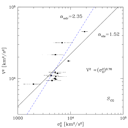
Figure 2: Virial velocity against the central velocity dispersion for each projection (dots) of a remnant; average values are indicated by solid squares. The solid line corresponds to an ols fit to the data obtained using a Sérsic growth-curve technique and $\xi\!=\!100\,$pc; the scaling expression for this case is indicated. The broken line represents the fit by odr. The slope of each line is indicated.

0.4.1 Velocities

In Figure 2 we plot, in log-space, $V^{2}$ against $\sigma^{2}_{0}$ for each projection (dots) of the remnants, where the average value of $\sigma_{0}^{2}$ is indicated by a larger symbol. An homologous behavior for the velocity scaling would require that $V^{2}\propto\sigma_{0}^{2}$.

Table 2: Velocity scalings $V^{2}\propto\sigma_{0}^{\alpha}$

$\xi$	$R^{1/4}_{\rm P}$	$R^{1/4}_{\rm{CG}}$	$S_{\rm P}$	$S_{\rm{CG}}$	FIT
100 pc	1.53	1.58	1.52	1.52	ols
	2.40	2.40	2.36	2.35	odr
1000 pc	1.46	1.54	1.48	1.46	ols
	2.30	2.40	2.33	2.30	odr

$R^{1/4}$ and $S$ indicate a de Vaucouleurs and Sérsic profile, respectively. Subscripts $\rm{P}$ and $\rm{GC}$ refer to whether a fitting to the surface density profile $\Sigma(R)$ or the curve of growth $M_{\rm L}(R)$ is done, and ols and odr refer to the type of least-squares fitting procedure used.

A relation of the form

$$V^{2}\propto\sigma_{0}^{\alpha}\,,$$ (9)

in log-space, was done to out data set. In Table 2 we list the results obtained for the $\alpha$ index under both fitting procedures odr and ols used, and both inner boundary radii $\xi$. The error in $\alpha$ by the ols procedure is $\pm 0.01$, while that for the odr procedure is $\pm 0.02$.

It can be noted that both fitting procedures (ols and odr) lead to different values for the $\alpha$ index. The odr procedure gives a value of $\alpha$ about 50% higher than that obtained by ols, under all the conditions used for the fittings.

Increasing $\xi$ in the fit leads to a small change ($\mathrel{\hbox to0.0pt{\lower 3.0pt\hbox{$\mathchar 536\relax$}\hss}\raise 2.0pt\hbox{$\mathchar 316\relax$}}\leavevmode\nobreak\ 5$%) in the $\alpha$ index for the same fitting procedure. At a fixed $\xi$, using the different fitting functions (profile or growth-curve), results in small variations ($<5$%) in the value of $\alpha$.

Averaging the results in Table 2, over $\xi$ and type of profile considered, we have for the ols procedure a $\langle\alpha\rangle_{\rm{ols}}=1.51$ while the odr approaches a value of $\langle\alpha\rangle_{\rm{odr}}=2.35$. In general, the values of $\alpha$ in our remnants deviate by $\approx 20$% from the homology expected value of $\alpha=2$. It follows from these results that our merger remnants do not satisfy kinematical homology.

We recall that the total (random plus rotational) kinetic energy of the system is related to $V^{2}$, and $\sigma_{0}^{2}$ is essentially a measure of random motion. The rather small departure from homology of $\alpha$ seems to suggest that the contribution from rotational energy might be small in the luminous part of the remnants. This result appears consistent with some observations of the rotational contribution to kinetic energy in ellipticals (e.g., Prugniel & Simien 1994).

However, to test the degree of rotational energy in our remnants a detailed kinematical analysis would be required, a topic that is under investigation at this time and to be presented in a future work.

0.4.2 Radii

In Figure 3 we plot the gravitational radius, $R_{\rm g}$, of each merger remnant versus their corresponding effective radii, $R_{\rm e}$, obtained from a fit using their Sérsic growth-curve with $\xi=100\,$pc, and considering all the randomly generated projections in the sky.

A fit in log-space of the form

$$R_{\rm g}\propto R_{\rm e}^{\beta}\,$$ (10)

was done. In Table 3 we list the different values of $\beta$ found under the different fittings conditions. Errors in $\beta$, under both the ols and odr, are $\pm 0.01$.

The $\beta$ values do not change ($\approx 20$%) as much as when the fit is done with an ols or an odr, in comparison to the $\approx 50$% change of the $\alpha$ index. An increase in $\beta$ of $\approx 20$% is obtained when the fitting is done on the profile using a $\xi=1\,$kpc instead of $100\,$pc. We note that when the growth-curve method is used the $\beta$ values decrease.

The $\beta$ index strongly depends on the adopted form of the fitting law, irrespectively of the fitting procedure. Its variation can be as much as $\approx 200$% when a Sérsic law is used instead of the $R^{1/4}$ law. This behavior is most probably related to the one observed in observational studies (e.g., Khosroshashi et al. 2004), where totally different values of $R_{\rm e}$ can be obtained if the brightness profile is not fitted by a suitable model. Here, the election of the adopted profile is reflected on the values of the $\beta$ index.

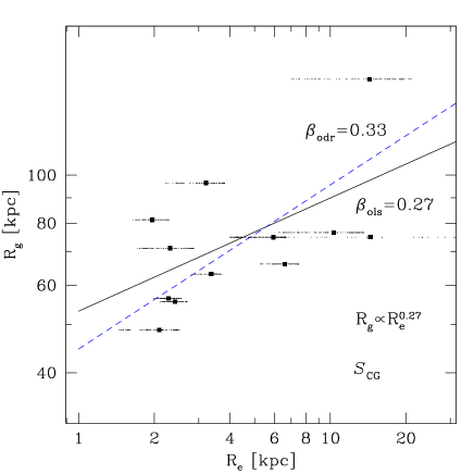
Figure 3: Similar as to Figure 2, but for the gravitational radius $R_{\rm g}$ and the effective radius $R_{\rm e}$.

Table 3: Radial scalings $R_{\rm g}\propto R_{\rm e}^{\beta}$

$\xi$	$R^{1/4}_{\rm P}$	$R^{1/4}_{\rm{CG}}$	$S_{\rm P}$	$S_{\rm{CG}}$	FIT
100 pc	0.09	0.16	0.27	0.27	ols
	0.11	0.19	0.33	0.33	odr
1000 pc	0.12	0.11	0.23	0.23	ols
	0.13	0.12	0.26	0.25	odr

Averaging all the values listed in Table 3 related to the de Vaucouleurs law, irrespective of the fitting procedure or $\xi$ value, we obtain a mean of $\langle\beta\rangle_{\rm{deV}}=0.13$, while for the Sérsic law a value of $\langle\beta\rangle_{\rm{S}}=0.27$ is obtained.

The dispersion of values, due to projection effects, around the mean value can be appreciated in Figure 3; where a Sérsic growth-curve method is used to determine $R_{\rm e}$. Although not shown, the dispersion around the mean value is somewhat larger when a $R^{1/4}$ profile is fitted.

The results obtained for the $\beta$ index, under all the fitting conditions considered, indicate a strong breaking of an homologous scaling between $R_{\rm g}$ and $R_{\rm e}$. In average, the $\beta$ index deviates $\approx 80$% away from the homology value of $\beta=1$.

0.4.3 Masses

In Figure 4 we plot the total mass of the remnant $M$ versus its luminous mass $M_{\rm L}$, where the latter was obtained using a fit to a Sérsic growth-curve and $\xi=100\,$pc.

A relation of the form

$$M\propto M_{\rm L}^{\gamma}$$ (11)

is assumed for the fitting in log-space of the data set. In Table 4 we list the values of the mass scaling index $\gamma$ for all the different fittings considered here. Errors in $\gamma$ in both procedures are $\pm 0.01$.

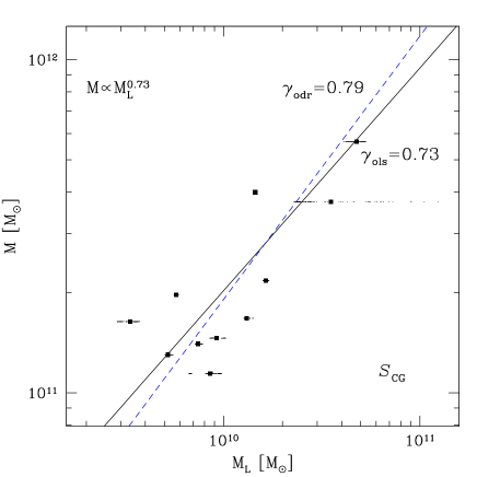
Figure 4: Similar to Figure 2, but for the total mass $M$ and the luminous mass $M_{\rm L}$ inferred from the fit.

The $\gamma$ index shows a smaller dispersion against projection effects in comparison to the $\alpha$ or $\beta$ indexes. This is probably related to the fact that $M_{\rm L}$ is an integrated quantity.

The mass index $\gamma$ shows the same tendency to increase its value when an odr fitting procedure is used in comparison to the ols one. Increasing the $\xi$ value has the effect of lowering the value of $\gamma$ in all cases considered, and is rather stable under the two laws of luminous matter distribution assumed (de Vaucouleurs or Sérsic). Averaging all values under the odr and ols procedures we find a $\langle\gamma\rangle_{\rm{odr}}=0.76$ and a $\langle\gamma\rangle_{\rm{ols}}=0.69$, respectively.

It is difficult to adequately transform our $M_{\rm L}$ to a luminosity $L$ in order to compare our results with observations, this due to the uncertainties on the mass-to-light ratios of ellipticals and the dissipationless nature of our simulations. Nonetheless, if we consider that $M\propto M_{\rm L}^{0.8}$, as provided by an odr fitting procedure using a Sérsic law with $\xi=100\,$pc, then the following total mass-to-luminous mass ratio is obtained:

$$\frac{M}{M_{\rm L}}\propto\frac{M_{\rm L}^{0.8}}{M_{\rm L}}\propto M_{\rm L}^{-0.2}\;.$$

Table 4: Mass scalings $M\propto M_{\rm L}^{\gamma}$

$\xi$	$R^{1/4}_{\rm P}$	$R^{1/4}_{\rm{CG}}$	$S_{\rm P}$	$S_{\rm{CG}}$	FIT
100 pc	0.69	0.76	0.72	0.73	ols
	0.78	0.84	0.79	0.79	odr
1000 pc	0.64	0.62	0.68	0.67	ols
	0.72	0.70	0.74	0.72	odr

Assuming a constant mass-to-light ratio, the previous result would imply that $M/L\propto L^{-0.2}$. Observationally it has been found, using a Sérsic profile (Trujillo, Burkert & Bell 2004), that $M/L\propto L^{0.06\pm 0.04}$. When comparing this result with the one obtained for our merger remnants, it follows that a constant mass-to-light ratio is not appropriate to reproduce the observational results.

Nevertheless, a constant mass-to-light ratio does not seem so unrealistic especially when mass-to-light ratios $\propto L^{-0.4}$ have been found for dwarf ellipticals (Peterson & Caldwell 1993). Such dependency is more closely reproduced, under a constant $M/L$ ratio, using other values of Table 4. However, a consistent comparison with observations requires additional physics not considered in this study.

0.5 Discussion and Conclusions

We have carried out twelve $N$-body simulations of binary mergers of disk galaxies, constructed using the galaxy formation model of MMW and with properties consistent with a Tully-Fisher realization at $z\!=\!1$. For the merger remnants, scaling relations among the physical quantities that appear in the virial theorem and their observationally related ones were obtained.

In particular we looked for relations of the form: $V\propto\sigma_{0}^{\alpha}$, $R_{\rm g}\propto R_{\rm e}^{\beta}$, and $M\propto M_{\rm L}^{\gamma}$. It is found that the scaling indexes are sensitive to the fitting procedure (odr or ols), to the inner starting radius of the fitting region, $\xi$, to the kind of law assumed to follow the luminous matter (de Vaucouleurs or Sérsic), and to whether a profile or growth-curve is used. The $\gamma$ index results to be the more stable under all these different fitting conditions.

In general, our results show that a strong breaking of homology occurs in dissipationless mergers. We find that the $\alpha$ and $\gamma$ indexes are more sensitive to the fitting procedure, obtaining for the ols procedure a $\langle\alpha\rangle_{\rm{ols}}=1.51$ and a $\langle\gamma\rangle_{\rm{ols}}=0.69$, while for the odr procedure $\langle\alpha\rangle_{\rm{odr}}=2.35$ and $\langle\gamma\rangle_{\rm{odr}}=0.76$. The $\beta$ index results to be more sensitive on the assumed law for luminous matter distribution, values $\langle\beta\rangle_{\rm{deV}}=0.13$ and $\langle\beta\rangle_{\rm{S}}=0.27$ are found.

An immediate consequence of our results is the existence of a non-linear scaling between the virial theorem, $M\propto V^{2}R_{\rm g}$, and its observational analogy, $M_{\rm L}\propto\sigma_{0}^{2}R_{\rm e}$. Moreover, the “constant” of proportionality between the physical and observational virial relations depends on the fitting procedure and the radial range where the fit is done. This indicates that care has to be taken when trying to obtain physical information from these observational parameters; for example, in determining the mass-to-light ratio of ellipticals using a kinematical approach based on the observational virial relation (e. g., Padmanabhan et al. 2004). Our results suggest that a dynamical mass estimate based on an homologous relation of the form $M_{\rm dyn}\propto\sigma_{0}^{2}R_{\rm e}$ is likely to be incorrect.

Properties of remnants depend on the angular momentum and energy of the orbit of the progenitors (e.g., Naab & Burkert 2003, González-García & Balcells 2005, Boylan-Kolchin, Ma & Quataert 2005). We expect that the scaling indexes, that reflect the breaking of homology in remnants, will also depend on these quantities. Boylan-Kolchin et al. (2005) address in an approximate manner, and with $N$-body simulations, the degree of homology breaking and find a dependence on the type of orbit considered. Although they just used one pericentric distance and a radial orbit, aside of using only spherical models, their result hints toward a dependency on angular momentum. Considering the small parameter space of simulations sampled out here, the values of $\{\alpha,\beta,\gamma\}$ obtained in this study are to be taken as indicative of the values they might attain under more general conditions. A complete study will require to study the dependence of the scaling indexes on the energy and angular momentum of the orbit, and needs to be addressed in the future.

Comparing our $N$-body results directly to observations is restricted by the uncertainties in transforming the luminous mass, $M_{\rm L}$, to luminosities, $L$. This is not an easy problem and would require to include, among other things, gas and stellar populations evolution models in the simulations. It is not clear at this stage how the scaling indexes would be affected by the inclusion of this new physics into the problem. However, in conclusion, it is clear from a purely $N$-body point of view that homology is not satisfied in merger remnants of spiral galaxies.

APPENDIX A

Orthogonal Fit to a Line

In the ordinary least-squares (ols) method errors in the “independent” variable are minimized. However, if there is no clear distinction which variable is dependent or independent a natural choice is to minimize errors in the normal direction to the surface fitted. This is the idea behind the orthogonal distance regression fitting (odr). We describe here the procedure used to fit a line by this method.

Let the line equation be described by

$${\bf L}={\bf X}_{0}+t{\bf{\bar{D}}}\;,$$ (12)

where ${\bf{\bar{D}}}$ is a unit length vector along the line and $t$ some scalar. If ${\bf X}_{i}$ is the 2-dimensional vector of the $n$ data points to be fitted, it can be written as

$${\bf X}_{i}={\bf X}_{0}+\zeta_{i}{\bf{\bar{D}}}+\varepsilon_{i}{\bf{\bar{D}}}^{\perp}\,,$$ (13)

where ${\bf{\bar{D}}}^{\perp}$ is a unit vector perpendicular to ${\bf{\bar{D}}}$ and $\zeta_{i}$, $\varepsilon_{i}$ are some scalars; see Figure 5.

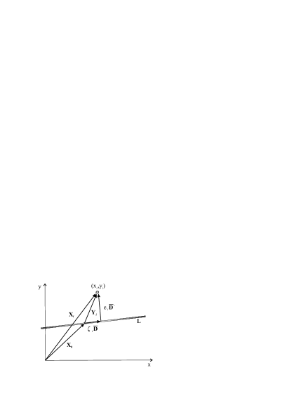
Figure 5: Schematic diagram indicating the quantities used for fitting a line to a set of data points by orthogonal distance regression (odr).

Let ${\bf Y}_{i}={\bf X}_{i}-{\bf X}_{0}$, then we have that

$${\bf Y}_{i}-\zeta_{i}{\bf{\bar{D}}}=\varepsilon_{i}{\bf{\bar{D}}}^{\perp}\;.$$

The function to be minimized in odr is

$$E({\bf X}_{0},{\bf{\bar{D}}})=\sum_{i=1}^{n}\varepsilon_{i}^{2}=\sum_{i=1}^{n}({\bf Y}_{i}-\zeta_{i}{\bf{\bar{D}}})^{2}\;.$$ (14)

We can write this as

$$E({\bf X}_{0},{\bf{\bar{D}}})=\sum_{i=1}^{n}[{\bf Y}_{i}^{T}({\bf 1}-{\bf{\bar{D}}}{\bf{\bar{D}}}^{T}){\bf Y}_{i}]\,.$$ (15)

The best fit ${\bf X}_{0}$ is obtained by setting

$$\frac{\partial E}{\partial{\bf X}_{0}}=-2({\bf 1}-{\bf{\bar{D}}}{\bf{\bar{D}}}^{T})\sum_{i=1}^{n}{\bf Y}_{i}=0\,,$$

that is obtained by setting $\sum_{i=1}^{n}({\bf X}_{i}-{\bf X}_{0})=0$, hence

$${\bf X}_{0}=\frac{1}{n}\sum_{i=1}^{n}{\bf X}_{i}=\left[\begin{array}[]{c}\langle x\rangle\\ \langle y\rangle\\ \end{array}\right]\,.$$ (16)

To obtain the best fit ${\bf{\bf D}}$ we find de minimum of the following equivalent expression to (15)

$$E({\bf X}_{0},{\bf{\bar{D}}})={\bf{\bar{D}}}^{T}\left\{\sum_{i=1}^{n}[({\bf Y}_{i}\cdot{\bf Y}_{i}){\bf 1}-{\bf Y}_{i}{\bf Y}_{i}^{T}]\right\}{\bf{\bar{D}}}\;,$$

and ${\bf 1}$ is the unit matrix. The term in brackets is a matrix, so we write this expression as

$$E({\bf X}_{0},{\bf{\bar{D}}})\equiv{\bf{\bar{D}}}^{T}M({\bf X}_{0}){\bf{\bar{D}}}\;.$$ (17)

Writing explicitly matrix $M({\bf X}_{0})$ we have

$$M({\bf X}_{0})=\left[\begin{array}[]{cc}\delta_{yy}^{2}&-\delta_{xy}^{2}\\ -\delta_{xy}^{2}&\delta_{xx}^{2}\\ \end{array}\right]\,,$$ (18)

where the $\delta_{xy}$ element is given by

$$\delta_{xy}^{2}=\sum_{i=1}^{n}\left(x_{i}-\langle x\rangle\right)\left(y_{i}-\langle y\rangle\right)\,.$$ (19)

From linear algebra we recognize the expression in (17) as a quadratic form. Its minimum value is provided by the eigenvector corresponding to the lowest eigenvalue of matrix (18). In particular, normalizing this eigenvector to unity leads us directly the components ${\bf{\bar{D}}}=(p,q)$, and hence the best fitted line (12). The line equation in parametric form can be written as

$$x=x_{0}+tp\;,\qquad y=y_{0}+tq\,,$$

and, eliminating the parameter $t$, we have the best line fitted by odr as:

$$y=\frac{q}{p}x+(y_{0}-\frac{q}{p}x_{0})\;.$$ (20)

Eigenvalues may be found by using Jacobi method (Press et al. 1992).

References

- (1) Aceves H., Velázquez H., 2005, MNRAS, 306, 50
- Barnes (1998) Barnes J. E., 1998, in Friedli D., Martinet L. and Pfenniger D., eds, Galaxies: Interactions and Induced Star Formation, Saas-Fee Advance Course 26, Springer-Verlag, New York
- (3) Bernardi M., Sheth R. K., Annis J., et al., 2003a, AJ, 125,1849
- (4) Bernardi M., Sheth R. K., Annis J., et al., 2003b, AJ, 125,1866
- (5) Bertin G., Ciotti L., Del Principe M., 2002, A&, 386, 149
- (6) Binggeli B., Jerjen H., 1998, A&A, 333, 17
- (7) Boylan-Kolchin M., Ma C., Quataert E., 2005, astro-ph/0502495
- (8) Burstein D., Davies R. L., Dressler A., Faber S. M., Stone R. P. S., Lynden-Bell D., Terlevich R. J., Wegner G., 1987, ApJS, 64, 601
- (9) Caon N., Capaccioli M., D’Onofrio M., 1993, MNRAS, 265, 1013
- (10) Chiosi C., Carraro G., 2002, MNRAS, 335, 335
- (11) Ciotti L., Bertin G., 1999, A&A, 352, 447
- (12) de Vaucouleurs G., 1948, Ann. d’Astroph., 11, 247
- (13) Efron B., R. J. Tibshirani R. J., 1993, An Introduction to the Bootstrap. Chappman & Hall., New York.
- (14) Efstathiou G., Lake G., Negroponte J., 1982, MNRAS, 199, 1069
- (15) Faber S. M., Jackson R. E., 1976, ApJ, 204, 668
- (16) Feigelson E. D., Babu G. J., 1992, ApJ, 397, 55
- (17) Giovanelli R., Haynes M. P., da Costa L. N., Freudling W., Salzer J. J., Wegner G., 1997, ApJ, 477, L1
- (18) González-García A. C., Balcells M., 2005, MNRAS, 357, 753
- (19) Graham A. W., 1998, MNRAS, 295, 933
- (20) Hernquist L., 1993, ApJS, 86, 389
- (21) Jørgensen I., Franx M., Kjaergaard P., 1996, MNRAS, 280, 167
- (22) Khosroshahi H. G., Raychaudhury S., Ponman T. J., Miles T. A., Forbes D. A., 2004, MNRAS, 349, 527
- (23) Kormendy J., 1977, ApJ, 217, 406
- (24) Mo H. J., Mao S., White S. D. M., 1998, MNRAS, 295, 319 (MMW)
- (25) Naab T., Burkert A., 2003, ApJ, 597, 893
- (26) Navarro J. F., Frenk C. S., White S. D. M., 1995, MNRAS, 275, 56
- (27) Navarro J. F., Frenk C. S., White S. D. M., 1997, ApJ, 490, 493
- (28) Padmanabhan N., Seljak U., Strauss M. A., et al., 2004, New Astronomy, 9, 329
- (29) Peebles P. J. E., 1993, Principles of Physical Cosmology. Princeton U. P., Princeton.
- (30) Peebles P. J. E., 2002, in Nigel Metcalfe & Tom Shanks Eds., A New Era in Cosmology, ASP Conference Proceedings, Vol 283, Astronomical Society of the Pacific, San Francisco
- (31) Peterson R. C., Caldwell N., 1993, AJ, 105, 1411
- (32) Power C., Navarro J. F., Jenkins A., Frenk C. S., White S. D. M., Springel V., Stadel J., Quinn T., 2003, MNRAS, 338, 14
- (33) Prugniel Ph., Siemen F., 1994, A&A, 282, L1
- (34) Prugniel Ph., Simien F., 1997. A&A, 321, 111
- (35) Press W. H., Teukolsy S. A., Vetterling W. T., Flannery B. P., 1992, Numerical Recipes. Cambridge Univ. Press, New York
- (36) Sérsic J. L., 1968, Atlas de Galaxias Australes. Observatorio Astronómico, Córdoba, Argentina
- (37) Shen S., Mo H. J., Shu C., 2002, MNRAS, 331, 251 (SMS)
- (38) Syer D., Mao S., Mo H. J., 1997, astro-ph/9711160
- (39) Springel V., Yoshida N., White S. D. M., 2001, New Astronomy, 6, 79
- Schweizer (1998) Schweizer F., 1998, in Friedli D., Martinet L. and Pfenniger D., eds, Galaxies: Interactions and Induced Star Formation, Saas-Fee Advance Course 26, Springer-Verlag, New York
- Toomre (1977) Toomre A., 1977 in Tinsley B. M. and Larson R. B., eds, The Evolution of Galaxies and Stellar Populations. Yale Univ. Obs., New Haven, p. 401
- (42) Tully R. B., Fisher J. R., 1977, A&A, 64, 661
- Trujillo et al. (2004) Trujillo I., Burkert A., Bell E. F., 2004, ApJ, 600, L39
- Velázquez & Aguilar (2003) Velázquez H., Aguilar L. 2003, RMxAA, 39, 197
- (45) Wu X., Fang L., Xu W., 1998, A&A, 338, 813