The evidence of absence: galaxy voids in the excursion set formalism

Abstract

We present an analytic model for the sizes of voids in the galaxy distribution. Peebles and others have recently emphasized the possibility that the observed characteristics of voids may point to a problem in galaxy formation models, but testing these claims has been difficult without any clear predictions for their properties. In order to address such questions, we build a model to describe the distribution of galaxy underdensities. Our model is based on the “excursion set formalism,” the same technique used to predict the dark matter halo mass function. We find that, because of bias, galaxy voids are typically significantly larger than dark matter voids and should fill most of the universe. We show that voids selected from catalogs of luminous galaxies should be larger than those selected from faint galaxies: the characteristic radii range from $\sim 5$–$10\,h^{-1}\mbox{ Mpc}$ for galaxies with absolute $r$-band magnitudes $M_{r}-5\log h<-16$ to $-20$. These are reasonably close to, though somewhat smaller than, the observed sizes. The discrepancy may result from the void selection algorithm or from their internal structure. We also compute the halo populations inside voids. We expect small haloes ($M\la 10^{11}\mbox{ M${}_{\odot}$}$) to be up to a factor of two less underdense than the haloes of normal galaxies. Within large voids, the mass function is nearly independent of the size of the underdensity, but finite-size effects play a significant role in small voids ($\la 7\,h^{-1}\mbox{ Mpc}$).

1 Introduction

One of the key predictions of any cosmological structure formation model is the distribution of matter on large scales. We now know that the cold dark matter (CDM) paradigm can account for many of the observed characteristics of the galaxy distribution. In this picture, the universe contained tiny (gaussian) density fluctuations at the time the cosmic microwave background was last scattered. Bound structures assembled themselves through gravitational instability around these perturbations in the relatively recent past. In the past two decades, with the advent of high-resolution numerical simulations, it has become possible to follow this picture through the formation of massive galaxies and clusters. The CDM model accurately describes the abundance and clustering of collapsed objects from dwarf galaxies to rich galaxy clusters over a wide range of redshifts (although the details of galaxy formation itself remain somewhat mysterious) as well as the distribution of neutral gas in the intergalactic medium.

These systems all correspond to density peaks in the matter distribution (with the exception of the lowest column density Ly$\alpha$ forest absorbers). For a variety of reasons, the other end of the density distribution – underdense voids – has received considerably less attention, despite their long observational history (Gregory & Thompson, 1978; Kirshner et al., 1981) and their place as the most visually striking features of the galaxy distribution. This is largely because voids subtend enormous volumes and so require large surveys to garner representative samples. Although voids have been found in every redshift survey (de Lapparent et al., 1986; Vogeley et al., 1994; El-Ad et al., 1997; El-Ad & Piran, 2000; Müller et al., 2000; Hoyle & Vogeley, 2002), the first statistically significant sample came only with the 2dF redshift survey (Hoyle & Vogeley, 2004). Now, with the DEEP2 redshift survey and the Sloan Digital Sky Survey, it is even possible to constrain the evolution of voids over the redshift interval $z\sim 1$–$0$ (Conroy et al., 2005).

Hoyle & Vogeley (2004) presented the most complete search for voids to date. They found that voids with characteristic radii $R\approx 15\,h^{-1}\mbox{ Mpc}$ fill $\sim 35\%$ of the universe. But their search illustrates a second difficulty in studying voids: how to define and identify them precisely (and meaningfully). El-Ad & Piran (1997) proposed the Voidfinder algorithm based on separating the observed galaxies into “void” and “wall” populations and building voids around gaps in the wall population (see also Hoyle & Vogeley 2002). While clearly defined for any given observational sample, the results can nevertheless be difficult to interpret in relation to the underlying physical quantities of interest. For example, the distribution of observed sizes depends on the galaxy sample (intrinsically brighter galaxies yield larger voids) as well as the search algorithm (Hoyle & Vogeley 2004 restrict their search to radii greater than $10\,h^{-1}\mbox{ Mpc}$, for example). Smaller voids are difficult to pinpoint because of confusion with random fluctuations in the galaxy distribution. We will nevertheless follow this approach and define a void to be any coherent region where the galaxy density falls below some threshold. Note that this differs from many other studies (e.g., Einasto et al. 1989; Gottlöber et al. 2003; Sheth & van de Weygaert 2004) that require a void to be completely empty of galaxies. These voids, which are much smaller than the voids we consider here, do not correspond to the voids detected by eye in the galaxy distribution.

The void phenomenon is also relatively difficult to study theoretically. The simplest model is a spherical tophat underdensity. The early evolution of such a system is well-described by spherical expansion (the analog of the well-known spherical collapse model; Peebles 1980). Underdensities expand in comoving units, gradually deepening, until they reach “shell-crossing,” when the center is evacuated and individual mass shells cross paths. At this stage, the initial spherical expansion model breaks down. Later, the voids continue to expand relatively slowly in a self-similar fashion (Fillmore & Goldreich, 1984; Suto et al., 1984; Bertschinger, 1985). Unfortunately, these dark matter models are idealizations in that real voids are observed only through the galaxy distribution. Because galaxies are biased relative to the dark matter, we must ask what kind of physical systems observed voids actually represent. They are in fact nearly empty of galaxies – but does that require shell-crossing, or can they be at an earlier evolutionary stage?

Another difficulty is that the large size of voids restricts the usefulness of numerical simulations. Early efforts focused on understanding the dynamics of individual voids, which did not require particularly high resolution (Dubinski et al., 1993; van de Weygaert & van Kampen, 1993). But placing voids in their proper cosmological context demands both large volumes and high mass resolution – the latter because we must resolve the galaxies from whose absence we identify voids (e.g., Goldberg & Vogeley 2004). Only recently have $N$-body simulations of the required dynamic range become practical. This has allowed the first systematic studies of the structure of large voids (Gottlöber et al., 2003) as well as of simulated voids in the dark matter distribution (Colberg et al., 2005) and in the galaxy distribution (Mathis & White, 2002; Benson et al., 2003). Nevertheless, there are still no full hydrodynamic simulations of the void phenomenon: galaxy properties are currently determined through semi-analytic models (Mathis & White, 2002; Benson et al., 2003).

There are a number of reasons to study the void phenomenon. Early attention focused on using the observed voids to constrain cosmological parameters. Blumenthal et al. (1992) and Piran et al. (1993) argued that the scale of typical voids would depend on the matter power spectrum, just as the abundance of clusters does. It was quickly realized that the void distribution seemed to have much more large-scale power than collapsed objects – most obviously, although voids with sizes $\ga 15h^{-1}\mbox{ Mpc}$ are not uncommon, collapsed objects do not reach the same mass scales. This is puzzling because an underdense region reaches shell-crossing only after the equivalent overdensity would virialize. Friedmann & Piran (2001) pointed out that a solution might lie in a proper treatment of the galaxies used to define voids: galaxy bias could lower the required dark matter underdensity, allowing voids to be larger for a given amount of CDM power. They argued that the observed population of large voids preferred a $\Lambda$CDM model.

Recently, interest in voids has focused on their role in galaxy formation. Peebles (2001) argued that (in the CDM model) voids should be populated by small dark matter haloes but that the observed voids appear to lack faint galaxies as well as bright ones. Is this a fundamental problem for the CDM paradigm, or does it indicate that galaxy formation proceeds differently in voids? One popular explanation is that photoheating during reionization may have suppressed the formation of dwarf galaxies in low-density environments (Tully et al., 2002; Barkana & Loeb, 2004; Cen, 2005), helping to clear faint galaxies from the voids. To study these problems, recent attention has focused on the variation of the galaxy luminosity function with the large-scale environment. Croton et al. (2005) and Hoyle et al. (2005) (see also Goldberg et al. 2005) found that the characteristic galaxy luminosity and the galaxy density both decrease significantly in low-density environments but that the faint-end slope remains nearly constant. The latter may be surprising given the expected variation in the halo mass function with environment.

Before we can answer any of these questions, however, we require a proper understanding of voids in CDM models. Mathis & White (2002) and Benson et al. (2003) made important strides forward with their studies of voids in $N$-body simulations. They claimed that current semi-analytic galaxy formation models predict void properties similar to those observed and argued that the conflict pointed out by Peebles (2001) was illusory. But such studies are still limited by their dynamic range and by the (necessarily complex) galaxy formation prescriptions imposed on the dark matter haloes.

The goal of this paper is to produce a straightforward analytic model of the void distribution and of galaxy populations within voids. Such a model will sharpen our understanding of voids in a CDM model and generate a baseline prediction with which we can contrast their observed properties. We will build on Sheth & van de Weygaert (2004), the most compelling theoretical model of voids to date. They used the excursion set formalism, which reproduces the abundance of collapsed haloes extremely well, to predict the distribution of void sizes. However, they required voids to reach shell-crossing and defined their properties in terms of the dark-matter underdensity. As a result, they predicted characteristic void radii much smaller than those observed. Our main goal is to modify their approach so as to describe voids in the galaxy distribution. Along the way, we will also be able to predict the halo populations within voids and quantify the claimed discrepancy with observational results.

The remainder of this paper is organized as follows. In §2, we examine the nonlinear evolution of the void density. Then, in §3, we show how to compute the linearized underdensity of voids with a specified galaxy underdensity, and we briefly discuss the expected galaxy populations inside voids. In §4, we show how to compute the cosmological abundance of large galaxy voids and compare our results to observations. Finally, we conclude in §5.

In our calculations, we assume a cosmology with $\Omega_{m}=0.3$, $\Omega_{\Lambda}=0.7$, $\Omega_{b}=0.046$, $H=100h\mbox{ km s${}^{-1}$ Mpc${}^{-1}$}$ (with $h=0.7$), $n=1$, and $\sigma_{8}=0.9$, consistent with the most recent measurements (Spergel et al., 2003).

2 The Gravitational Expansion of Voids

Because the principal quantity of interest is the physical volume of voids, we first describe how they expand beyond their initial comoving size. We will follow the method of Friedmann & Piran (2001). We consider the expansion of a tophat density perturbation that begins with a (negative) density perturbation $\delta_{i}$ inside a physical radius $R_{i}$ at an initial time $t_{i}$ (corresponding to $z_{i}$). If we assume zero peculiar velocity perturbation and consider only the epoch before shell-crossing (so that the mass inside of each shell is conserved), conservation of energy yields the equation of motion (Peebles, 1980)

$$\dot{R}^{2}(t) = H_{0}^{2}[-\Omega_{0}(1+z_{i})^{3}R_{i}^{2}\delta_{i}$$ (1)

$$+\Omega_{0}(1+z_{i})^{3}(1+\delta_{i})R_{i}^{3}/R(t)+\Omega_{\Lambda}R(t)^{2}],$$

where the first term on the right hand side is (twice) the initial total energy of the shell, the second term is (twice) the gravitational potential energy at time $t$, and the last term is (twice) the excess energy from the cosmological constant. We solve this equation for the physical radius of the shell as a function of time or redshift. The solution is such that the void expands in comoving units once nonlinear effects set in. We define

$$\eta\equiv\frac{R(1+z)}{R_{i}(1+z_{i})}$$ (2)

to be the ratio of the comoving size at redshift $z$ to its initial comoving size. The real fractional underdensity due to gravitational expansion is thus $1+\delta=\eta^{-3}$. Note that this is independent of $R_{i}$.

Equation (1) includes nonlinear expansion, but most of the following will be phrased in terms of the equivalent linear density $\delta^{L}$ extrapolated to the present day. (For clarity, we will denote all linear-extrapolated densities with a superscript “L” in the following.) In order to transform to physical densities and scales, we require $\eta(\delta^{L})$ or equivalently $\delta(\delta^{L})$. We therefore also compute the density as if linear theory were always accurate. Any perturbation can be divided into growing and decaying modes; in linear theory the growing mode (which is of course the only component surviving to the present day) obeys (Heath, 1977)

$$\delta^{L}=\frac{3\delta_{i}H(z)}{5}\int_{z}^{\infty}{\rm d}u\frac{u+1}{H^{3}(1/u-1)},$$ (3)

where $H^{2}(z)=\Omega_{0}(1+z)^{3}+\Omega_{\Lambda}$ in a flat universe. The constant $3/5$ comes from our choice of initial conditions: a perturbation with zero peculiar velocity has $60\%$ of its amplitude in the growing mode and the remainder in the decaying mode (Peebles, 1980).

We show the relation between the linearized and physical underdensities with the solid line in Figure 1. At first, while linear evolution is accurate, $\delta\approx\delta^{L}$, but then the physical underdensity flattens out and even a small deepening of the void corresponds to a large increase in $|\delta^{L}|$. The dashed line in Figure 1 shows a fitting function for $\delta(\delta^{L})$ from eq. (18) of Mo & White (1996). Although those authors were interested in $\delta>0$, the formula is accurate to a few per cent in the underdense regime as well. For reference, shell-crossing occurs at $\delta^{L}=-2.8$, corresponding to a physical underdensity $\delta=-0.81$. Beyond this point, our model for $\eta$ breaks down because the enclosed mass no longer remains constant. The expansion then proceeds self-similarly, with the comoving radius $R\propto a^{1/3}$ in an Einstein-de Sitter universe (Fillmore & Goldreich, 1984; Suto et al., 1984; Bertschinger, 1985), significantly slower than the expansion before shell-crossing. As a result, the void volume fraction will be dominated by regions that have not yet (or have just) reached shell-crossing (Blumenthal et al., 1992): deeper perturbations are rarer in the CDM model and can be neglected because they expand so slowly. We therefore do not consider the later evolution in any more detail.

For completeness, we also note that Figure 1 is nearly independent of the input cosmological parameters; differences in the cosmology manifest themselves in the growth rate of $\delta^{L}$ rather than in the function $\delta(\delta^{L})$ (Friedmann & Piran, 2001).

Figure 1: Physical dark matter underdensity $\delta$ as a function of the linearized underdensity $\delta^{L}$ (solid line). Note that our model actually breaks down for $\delta<-0.81$, when shell-crossing occurs (marked by the horizontal dotted line). The dashed line shows the fitting function of Mo & White (1996).

3 Defining Voids

It may now seem straightforward to compute the void distribution: one simply chooses a physical density threshold $\delta$, transforms to $\delta^{L}$, and uses the excursion set formalism to determine the mass distribution of objects with the specified linearized underdensity (Sheth & van de Weygaert, 2004). While such a procedure is perfectly well-defined, it has one crucial shortcoming: in observed samples, we do not define voids in terms of their dark matter density but in terms of their galaxy density. Thus we actually want to relate the physical galaxy underdensity $\bar{\delta}_{\rm gal}$ within some region to $\delta^{L}$. That is the task of this section.

3.1 The galaxy mass function

Table 1: Mass Thresholds and Survey Depths

$M_{r}-5\log h$	$M_{b_{J}}-5\log h$	$n\,(10^{-3}\,h^{3}\mbox{ Mpc${}^{-3}$})$	$m_{\rm min}$ (PS; $10^{11}\mbox{ M${}_{\odot}$}$)	$m_{\rm min}$ (ST; $10^{11}\mbox{ M${}_{\odot}$}$)
-16	-16.3	58.6	1.0	0.73
-18	-17.8	27.9	2.5	1.7
-19	-18.7	15.2	5.2	3.4
-20	-19.5	5.89	15	10
-21	-20.4	1.11	90	60

Number densities are computed from the Blanton et al. (2003) $r$-band and Croton et al. (2005) $b_{J}$-band luminosity functions. Columns 4 and 5 give the minimum halo mass required to match these densities, with the Kravtsov et al. (2004) $\left\langle N(m_{h})\right\rangle$, for the Press-Schechter and Sheth-Tormen mass functions, respectively.

We will use the excursion set formalism to derive the dark matter halo mass function (Bond et al., 1991). In the simplest such model, a halo of mass $m_{h}$ forms whenever the smoothed density field first exceeds a linear-extrapolated density $\delta^{L}_{c}$ that is fixed by the physics of spherical halo collapse ($\delta^{L}_{c}=1.69$ for objects collapsing at the present day; Peebles 1980). To solve such a problem, we consider diffusion in the $(\delta^{L},\,\sigma^{2})$ plane, where $\sigma^{2}$ is the variance of the density field smoothed on scale $m_{h}$. Trajectories begin with $\delta^{L}=0$ at $\sigma^{2}=0$ (i.e., they must have the mean density on infinitely large scales). They then diffuse away from the origin as density modes are added on smaller scales. The problem is simply to compute the distribution of $\sigma^{2}$ (or equivalently $m_{h}$) at which these trajectories cross the absorbing barrier $\delta^{L}_{c}$ for the first time. From this first-crossing distribution, the mean comoving number density of haloes with masses $m_{h}\pm{\rm d}m_{h}/2$ is (Press & Schechter, 1974; Bond et al., 1991)

$$n_{h}(m_{h})=\sqrt{\frac{2}{\pi}}\,\frac{\bar{\rho}}{m_{h}^{2}}\,\left|\frac{{\rm d}\ln\sigma}{{\rm d}\ln m_{h}}\right|\,\frac{\delta^{L}_{c}}{\sigma}\,\exp\left[-\frac{(\delta^{L}_{c})^{2}}{2\sigma^{2}}\right],$$ (4)

where $\bar{\rho}$ is the mean matter density. In a region with linearized underdensity $\delta^{L}_{v}$ and mass $M_{v}$ [with $M_{v}=(4\pi/3)\,\bar{\rho}\,(R_{v}/\eta)^{3}$ for a void], the comoving number density of haloes is (Bond et al., 1991; Lacey & Cole, 1993)

$$n_{h}(m_{h}|\delta^{L}_{v},M_{v}) = \sqrt{\frac{2}{\pi}}\,\frac{\bar{\rho}}{m_{h}^{2}}\,\left|\frac{{\rm d}\ln\sigma}{{\rm d}\ln m_{h}}\right|\,\frac{\sigma^{2}(\delta^{L}_{c}-\delta^{L}_{v})}{(\sigma^{2}-\sigma^{2}_{v})^{3/2}}$$ (5)

$$\times\exp\left[-\frac{(\delta^{L}_{c}-\delta^{L}_{v})^{2}}{2(\sigma^{2}-\sigma^{2}_{v})}\right],$$

where $\sigma_{v}\equiv\sigma(M_{v})$ and of necessity $\sigma>\sigma_{v}$. This conditional mass function follows from an identical diffusion problem, but in this case the trajectories begin at $(\delta^{L}_{v},\sigma^{2}_{v})$ rather than the origin.

Although equation (4) provides a reasonable match to halo abundances in cosmological simulations, it is by no means perfect. Sheth & Tormen (1999) and Jenkins et al. (2001) provide more accurate fits to the simulation results. We will nevertheless use the standard Press-Schechter abundances in the following. The main reason is that, although the Sheth-Tormen mass function can also be motivated by a diffusion problem with the absorbing barrier fixed by ellipsoidal collapse, there is no analytic form for the conditional mass function because the barrier changes its effective shape with a shift of the origin. Sheth & Tormen (2002) showed that the conditional mass function could be approximated through a Taylor series, but in that case the corresponding unconditional mass function differs slightly from the usual Sheth-Tormen form (which provides the best match to numerical simulations). Zhang & Hui (2005) showed how to derive the mass function corresponding to such barriers using a simple numerical scheme. But for our purposes the Press-Schechter form suffices. The most important property is the density dependence. Barkana & Loeb (2004) and Furlanetto et al. (2005) found that it is extremely similar to that contained in equation (5), at least at high redshifts, and the former also showed that it fits simulations fairly well.

Equations (4) and (5) give the dark matter halo abundance, which is not the same as the galaxy abundance. To connect the two we require the mean number of galaxies per halo, $\left\langle N(m_{h})\right\rangle$, the first moment of the halo occupation distribution. For simplicity, we will use the universal form of Kravtsov et al. (2004). They split the mean occupation number into two parts. The first, $\left\langle N_{c}(m_{h})\right\rangle$, represents the number of central galaxies in the halo and is unity if $m_{h}>m_{\rm min}$ and zero otherwise. We will normally choose $m_{\rm min}$ by comparison to some observational detection threshold; note therefore that it need not reflect the actual minimum mass of a galaxy. The second part, $\left\langle N_{s}(m_{h})\right\rangle$, describes the number of satellite galaxies above the same detection limit. Kravtsov et al. (2004) found that this has a simple form

$$\left\langle N_{s}(m_{h})\right\rangle=\left(\frac{m_{h}}{C\,m_{\rm min}}\right)^{\beta}.$$ (6)

From fits to the subhalo distribution in $N$-body simulations, they estimate that $C\approx 30$ and $\beta\approx 1$ at $z=0$ over a broad range of halo masses. We will use these fiducial values in most of our calculations. In order to estimate the importance of the halo occupation distribution, we will also compare to a model with $\left\langle N(m_{h})\right\rangle=1$.

The total comoving number density of (observable) galaxies within a region is therefore

$$n_{g}^{c}(m_{\rm min}|\delta^{L}_{v},M_{v})=\int_{m_{\rm min}}^{\infty}{\rm d}m_{h}\,\left\langle N(m_{h})\right\rangle\,n_{h}(m_{h}|\delta^{L}_{v},M_{v}),$$ (7)

where the superscript “c” denotes a cumulative quantity. We wish to compare to voids selected through galaxy surveys. We will therefore set $m_{\rm min}$ by comparison to the galaxy number densities in the Sloan Digital Sky Survey and the 2dF Galaxy Redshift Survey. Specifically, we match to the number density of galaxies with $r$-band luminosity greater than a specified value, using the luminosity function of Blanton et al. (2003), and to the corresponding quantities from the $b_{J}$-band luminosity function of Croton et al. (2005). The appropriate mass thresholds $m_{\rm min}$ for the Press-Schechter and Sheth-Tormen mass functions are shown in Table 1. We will also show some results for $m_{\rm min}=10^{10}\mbox{ M${}_{\odot}$}$ in order to mimic an exceptionally deep survey. Note that normalizing in this way – to the cumulative number density of galaxies – tends to wash out differences between mass functions, insulating us from much of the uncertainty in using the Press-Schechter mass function.

3.2 The linearized underdensity of voids

The total (observed) galaxy underdensity in a void with physical size $R_{v}$ is

$$1+\bar{\delta}_{\rm gal}(m_{\rm min},\delta^{L}_{v},R_{v})=\frac{n_{g}^{c}(m_{\rm min}|\delta^{L}_{v},M_{v})}{\eta^{3}\,n_{g}^{c}(m_{\rm min})}.$$ (8)

Given $m_{\rm min}$, we solve this equation to find the linearized underdensity required to produce a void of size $R_{v}$ and mean observed galaxy underdensity $\bar{\delta}_{\rm gal}$.

Figure 2 shows the results of this inversion. The solid curves in panel (a) give the required underdensity for several different survey depths: $M_{r}<-20,\,-18,\,-16$, and $m_{h}>10^{10}\mbox{ M${}_{\odot}$}$, from top to bottom. (Here and throughout, we will suppress the “$-5\log h$” in measured magnitudes for the sake of brevity.) We take $\bar{\delta}_{\rm gal}=-0.8$ as a fiducial value. We plot $\delta^{L}_{v}$ as a function of mass variance $\sigma^{2}$. For reference, $\sigma^{2}=0.4,\,1.9$, and $4$ correspond to comoving sizes $R\approx 15,\,5$, and $2.5h^{-1}\mbox{ Mpc}$, respectively. Note that this is not the physical size of the void (which is larger by a factor $\eta$ and varies with $\delta^{L}_{v}$). We halt each curve at $M_{v}=2m_{\rm min}$. The required underdensity becomes more extreme in deeper surveys; this is because underdense regions are much more deficient in massive galaxies than small haloes in the extended Press-Schechter formalism. Haloes with masses $m_{h}\la M_{v}$ cannot collapse because too few density modes are available between $(M_{v},\,m_{h})$ to pass the collapse threshold $\delta^{L}_{c}$, but if $\sigma^{2}\gg\sigma_{v}^{2}$ (for small haloes) the loss of large-scale power becomes unimportant. In other words, the bias increases with galaxy mass, so the large galaxies are more sensitive to the underlying density field (Efstathiou et al., 1988; Cole & Kaiser, 1989; Mo & White, 1996). This is why $\delta^{L}_{v}$ curves upward as $\sigma^{2}$ increases, especially in the $M_{r}<-20$ case. There is also a slight trend for $\delta^{L}_{v}$ to increase as $\sigma\rightarrow 0$; this is because the shape of the mass function changes in underdense regions, with more mass in small haloes. As the void size approaches infinity, slightly more of the mass shifts into galaxy-mass haloes.

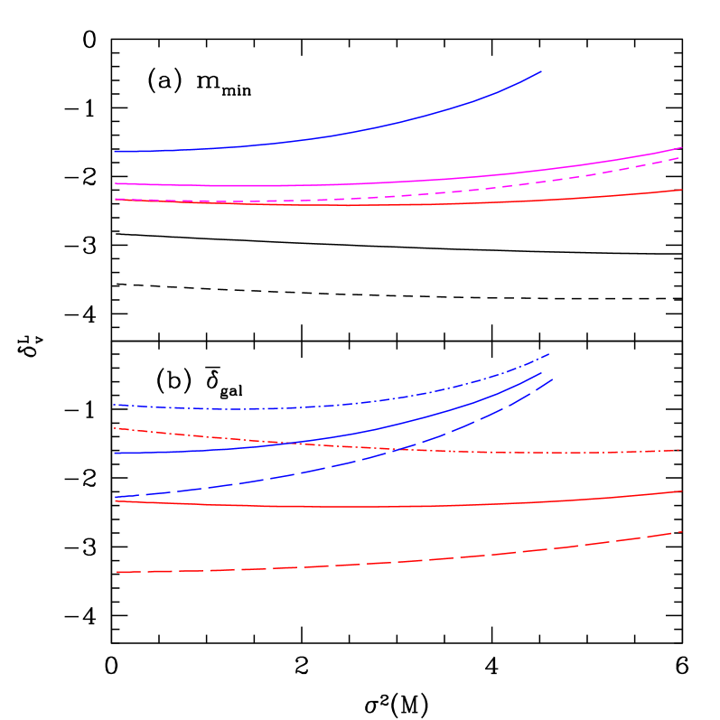
Figure 2: Linearized underdensity $\delta^{L}_{v}$ required to produce a mean (physical) galaxy underdensity $\bar{\delta}_{\rm gal}$. (a): All curves assume $\bar{\delta}_{\rm gal}=-0.8$. The solid curves use our fiducial model, with $M_{r}<-20,\,-18,\,-16$, and $m_{h}>10^{10}\mbox{ M${}_{\odot}$}$, from top to bottom. The dashed curves assume one galaxy per dark matter halo; we show $M_{r}<-18$ and $m_{h}>10^{10}\mbox{ M${}_{\odot}$}$. (b): The dot-dashed, solid, and dashed curves assume $\bar{\delta}_{\rm gal}=-0.6,\,-0.8$, and $-0.9$, respectively. We show results for $M_{r}<-20,\,-16$ (top and bottom sets of curves).

The two dashed curves in Figure 2a show $\delta^{L}_{v}$ if we assume $\left\langle N(m_{h})\right\rangle=1$ for $M_{r}<-18$ and $m_{h}>10^{10}\mbox{ M${}_{\odot}$}$. This decreases the threshold, because it increases the weight of the smallest haloes (which are least sensitive to the density). The value of $\delta^{L}_{v}$ becomes more sensitive to the halo occupation number for deeper surveys; a larger minimum mass pushes the survey to the steep part of the mass function, where the extra satellites in extremely large (but rare) haloes make only a small difference. Note as well that in this case the $m_{h}>10^{10}\mbox{ M${}_{\odot}$}$ threshold lies significantly below shell-crossing, where our model breaks down.

Figure 2b varies $\bar{\delta}_{\rm gal}$ for $M_{r}<-20$ and $M_{r}<-16$ (top and bottom sets of curves). We let $\bar{\delta}_{\rm gal}=-0.6,\,-0.8$, and $-0.9$ for the dot-dashed, solid, and dashed curves. This obviously has a strong effect on $\delta^{L}_{v}$, because the massive galaxies are so sensitive to the underlying dark matter density. Note that the differences are largest at small $\sigma^{2}$ (or large physical scales), because at smaller scales the finite size of the void limits the maximum halo mass. This is also why the differences are larger for the deeper survey.

3.3 Haloes in voids

Now that we have defined voids, we can look more closely at their resident halo populations. Figure 2 clearly shows that the intrinsic properties of voids depend sensitively on the mass limit of the survey used to detect them: deeper surveys require larger dark matter underdensities and hence will presumably find smaller voids. But, in a given void, will smaller haloes be more abundant relative to the (brighter) galaxy population used to define the void? To answer this question, we let

$$1+\delta_{h}(m)=\frac{n_{h}(m|\delta^{L}_{v},M_{v})}{\eta^{3}\,n_{h}(m)}.$$ (9)

We emphasize that $\delta_{h}$ is the halo underdensity at mass $m$, not the galaxy underdensity. The analogous galaxy underdensity at a particular mass is more difficult to calculate, because it requires the distribution of galaxy masses within each halo instead of simply the number of galaxies (i.e., how many satellite galaxies of mass $m$ are contained in any galaxy group). Such models require considerably more machinery than is appropriate for our simple analytic model. We will therefore content ourselves with computing the halo distribution, which will illustrate the most important features anyway. We will comment on its relation to the galaxy population below.

Figure 3 shows predictions for the halo underdensity in voids with $R_{v}=21\,h^{-1}\mbox{ Mpc}$. The parameters in the two panels are identical to those in Figure 2. In panel (a), we see that small haloes become less underdense if void selection is performed with larger galaxies. Within any given void, we also see that small haloes are less underdense than large haloes. This is, of course, because larger haloes are more biased than small ones. The disparity can be quite large for the $M_{r}<-20$ sample, with small haloes only half as underdense as those with $m_{h}\approx 10^{13}\mbox{ M${}_{\odot}$}$. The dashed curves show that these conclusions are qualitatively independent of $\left\langle N(m_{h})\right\rangle$. In panel (b), we see that varying $\bar{\delta}_{\rm gal}$ also modifies the fractional overdensity. However, its effects on the shape of the curve are relatively modest except at the most massive end.

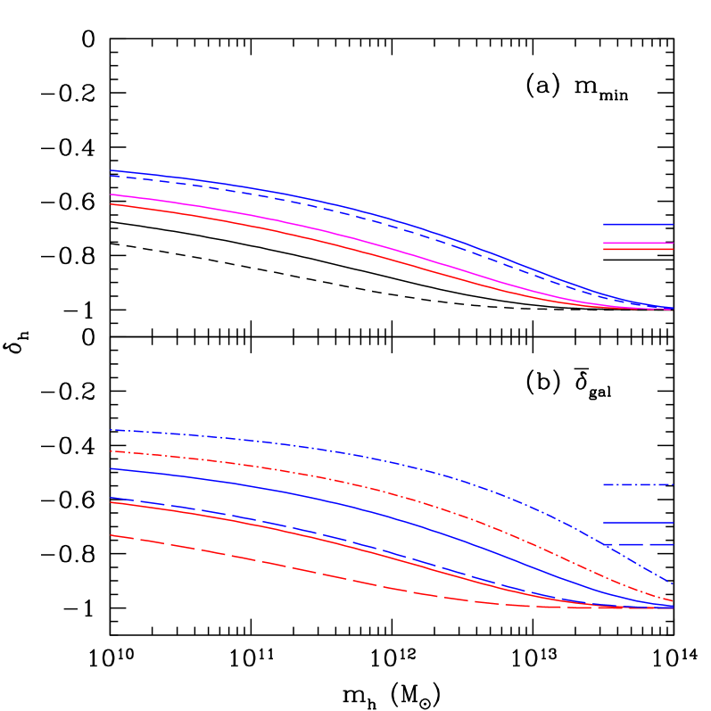
Figure 3: Underdensity of haloes within voids of physical size $R_{v}=21\,h^{-1}\mbox{ Mpc}$. (a): Assumes $\bar{\delta}_{\rm gal}=-0.8$. The solid curves use our fiducial model, with $M_{r}<-20,\,-18,\,-16$, and $m_{h}>10^{10}\mbox{ M${}_{\odot}$}$, from top to bottom. The horizontal bars on the right show $\delta$ in each of these voids (same ordering from top to bottom). The dashed curves assume one galaxy per dark matter halo; we show $M_{r}<-20$ and $m_{h}>10^{10}\mbox{ M${}_{\odot}$}$. (b): The dot-dashed, solid, and dashed curves assume $\bar{\delta}_{\rm gal}=-0.6,\,-0.8$, and $-0.9$, respectively. We show results for $M_{r}<-20,\,-16$ (top and bottom sets of curves). The horizontal bars show the corresponding $\delta$ for the $M_{r}<-20$ cases.

The horizontal bars on the right axis of Figure 3 show the physical dark matter underdensity within each void. Interestingly, it takes a relatively narrow range of values in panel (a), clustered around $\delta\approx-(0.7$–$0.8$), with $|\delta|$ decreasing as $m_{\rm min}$ increases. The halo populations (especially at large masses) spread over a much broader range in $\delta_{h}$. This is essentially a consequence of the shape of $\delta(\delta^{L})$ shown in Figure 1: a narrow range in physical underdensities spans a large range of $\delta^{L}$, which is the quantity relevant to our model for halo abundances. In general, $\delta\sim\delta_{h}$ for haloes selected near $m_{\rm min}$. The density of haloes with $m\ll m_{\rm min}$ is closer to the mean because their bias is less than unity.

Our model also predicts that $\delta_{h}$ at a fixed mass will vary with the size of the void, because $\delta^{L}_{v}$ is also a function of scale. We show the implications in Figure 4; in this case we consider surveys with $M_{r}<-19$ and $M_{r}<-16$ (top and bottom sets, respectively). For large voids, $R_{v}\ga 7\,h^{-1}\mbox{ Mpc}$, we see only a slight steepening of the curves, which occurs because the finite mass of the void limits the maximum halo mass. Thus, galaxy populations in voids with $R_{v}\ga 7\,h^{-1}\mbox{ Mpc}$ should be nearly independent of the void radius. This is a consequence of the flatness of $\delta^{L}_{v}$ at small $\sigma^{2}$ in Figure 2, which occurs because so little power exists on such large physical scales. However, when $R_{v}\sim 2.1\,h^{-1}\mbox{ Mpc}$, the shapes change dramatically because the finite size of the void strongly limits the haloes inside. A comoving volume with radius $R=2.1\,h^{-1}\mbox{ Mpc}$ contains $\sim 10^{13}\mbox{ M${}_{\odot}$}$, which is only $\sim 20$–$100$ times larger than the mass limits of these surveys. Thus the region requires only a modest underdensity to decrease the abundance of massive galaxies. Such “voids” therefore sit near the mean density and smaller haloes (for which finite size effects can be neglected) will have nearly their mean density. This simplified model suggests that many properties of voids will depend on their spatial extents, at least if $R_{v}\la 7h^{-1}\mbox{ Mpc}$.

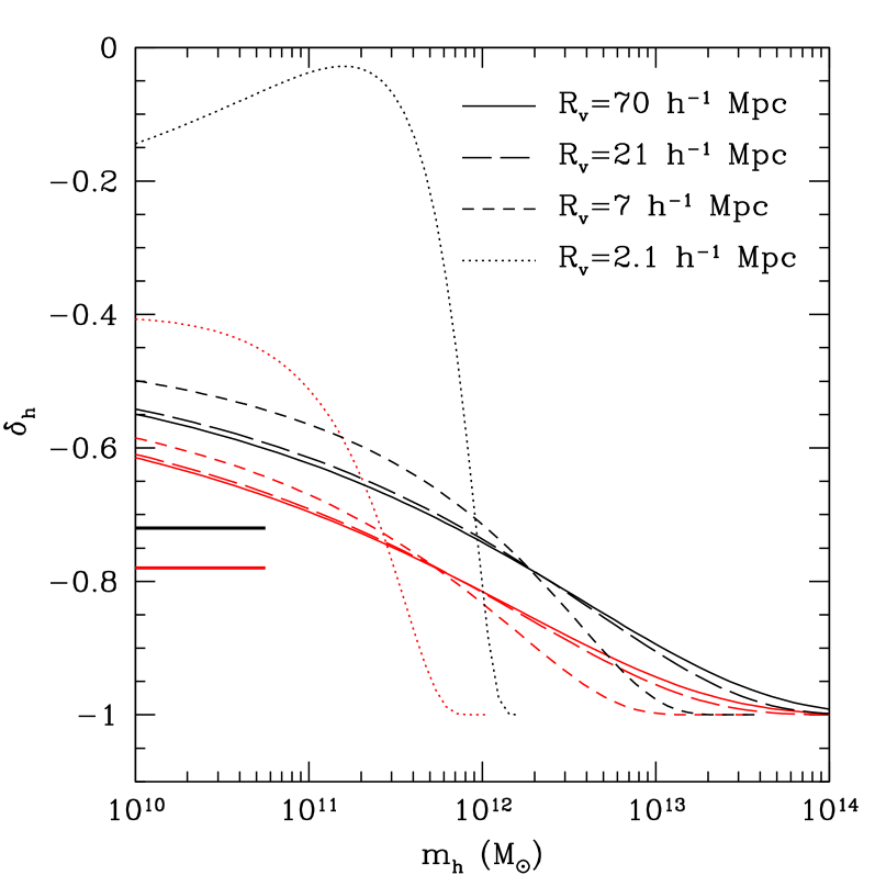
Figure 4: Underdensity of haloes within voids of $\bar{\delta}_{\rm gal}=-0.8$ and several different radii. The upper thick and lower thin sets of curves assume $M_{r}<-19$ and $-16$, respectively. The horizontal bars at left show $\delta$ for $R_{v}=7\,h^{-1}\mbox{ Mpc}$ voids.

One consistent theme of this section is that large haloes are relatively less abundant than small haloes within voids. We can compare this expectation to observations, which suggest that the mean number density $\bar{n}_{\rm gal}$ and the characteristic luminosity $L_{\star}$ decrease significantly in voids but that the faint-end slope of the luminosity function remains nearly constant (Croton et al., 2005; Hoyle et al., 2005). Unfortunately, the comparison is not trivial. These studies measured the galaxy environment through the mean density within spheres of size $\sim 8\,h^{-1}\mbox{ Mpc}$ (generally by comparing to the density field of a volume-limited sample of galaxies). This is just large enough that finite size effects should not be dramatic, but it is still in a regime in which Poisson fluctuations in the galaxy distribution cannot be neglected. As a result, some of the “low-density” regions may in fact be at the mean density, which would wash out the void effect. An ideal test would focus on those galaxies identified to be within large voids (for example using the Voidfinder algorithm). Moreover, we must also bear in mind that $\delta_{h}\neq\delta_{\rm gal}$. In particular, many small galaxies will be satellites inside large haloes; such a population will be efficiently suppressed in just the same way as bright central galaxies. Thus we expect the galaxy luminosity function in voids to be flatter than the halo mass function.

With these caveats, our model naturally explains the decrease in $\bar{n}_{\rm gal}$ and $L_{\star}$, especially because these regions are relatively small and finite size effects help suppress galaxies with $m\ga 10^{12}\mbox{ M${}_{\odot}$}$. Note that this probably explains the discrepancy between the observed $L_{\star}$ and that predicted by Cooray (2005), who let $R_{v}\rightarrow\infty$ rather than including a cutoff at $R_{v}\sim 8h^{-1}\mbox{ Mpc}$ which would have quenched the formation of massive galaxies. On the other hand, our models robustly predict an excess (by about a factor of two) between the abundance of small and large haloes in voids. If there were a one-to-one correspondence between halo mass and galaxy luminosity, and if the luminosity function could be approximated by a power law $n\propto L^{-\alpha}$ over this interval, we would expect $\alpha$ to be $\sim 0.15$ larger in voids than in mean density environments. The suppression of satellite galaxies would reduce the disparity. Even so, our result is within the error bars of Croton et al. (2005), though their best-fit values indicate no significant change. Thus, there is currently only weak evidence, at best, for non-standard galaxy formation within voids. CDM models robustly predict an excess of small haloes inside of voids, but it is not particularly strong and requires care to interpret.

4 Void Abundances

4.1 The excursion set abundance

Sheth & van de Weygaert (2004) used the excursion set formalism to estimate the number density of voids. They defined a void as a region with dark matter underdensity $\delta^{L}_{v}$. At first sight, the void abundance seems to follow from equation (4), but with $\delta^{L}_{c}\rightarrow\delta^{L}_{v}$: this is the same problem as the halo abundance, except that the absorbing barrier is negative rather than positive. However, Sheth & van de Weygaert (2004) pointed out one crucial difference, which they called the “void-in-cloud” problem. Consider a small region with $\delta^{L}<\delta^{L}_{v}$ that is contained in a larger region with $\delta^{L}>\delta^{L}_{c}$. Equation (4) would have assigned such a point to a small void; however, physically we know that this “void” lies inside of a collapsed object and hence has been crushed out of existence. (This problem does not occur for $n_{h}$ because haloes are allowed to collapse inside voids.)

Thus, the appropriate diffusion problem has two barriers: we wish to compute the first-crossing distribution for the void barrier $\delta^{L}_{v}$ while excluding trajectories that have already crossed a barrier with $\delta^{L}_{p}>0$ that describes void-crushing. The simplest assumption is to take both these barriers to be independent of $\sigma^{2}$; in that case Sheth & van de Weygaert (2004) showed that the mass function is (see also the alternate derivation in the Appendix)

$$n_{v}(m_{v}) = \frac{\bar{\rho}}{m_{v}^{2}}\,\left|\frac{{\rm d}\ln\sigma}{{\rm d}\ln m_{v}}\right|\sum_{n=1}^{\infty}\left\{\frac{n^{2}\pi^{2}D^{2}}{(\delta^{L}_{v}/\sigma)^{2}}\,\frac{\sin(n\pi D)}{n\pi}\right.$$ (10)

$$\times\left.\exp\left[-\frac{n^{2}\pi^{2}D^{2}}{2(\delta^{L}_{v}/\sigma)^{2}}\right]\right\},$$

where

$$D\equiv\frac{|\delta^{L}_{v}|}{\delta^{L}_{p}+|\delta^{L}_{v}|}$$ (11)

describes the relative importance of void-crushing; a fraction $(1-D)$ of all matter lies inside voids in this model. Note that $\delta^{L}_{v}$ and $\delta^{L}_{p}$ implicitly depend on redshift, because we evaluate $\sigma$ at the present day.

The Sheth & van de Weygaert (2004) model contains one crucial assumption – that voids can be defined at a constant $\delta^{L}_{v}$, independent of scale – and two free parameters. In what follows we will usually set the void-crushing parameter $\delta^{L}_{p}=1.06$, which is the linearized overdensity at turnaround according to the spherical collapse model. This is reasonable because it marks the point at which larger scale overdensities will begin to collapse around their resident voids, but we will also let $\delta^{L}_{p}$ take larger values for illustrative purposes. The second free parameter is $\delta^{L}_{v}$; Sheth & van de Weygaert (2004) argued that $\delta^{L}_{v}=-2.8$ (shell-crossing) is an appropriate choice, because that marks the maximum point of efficient expansion.

However, we have already seen that the dark matter underdensity is generally significantly deeper than the galaxy underdensity. Instead, if one wishes to compare to voids observed in redshift surveys, $\delta^{L}_{v}$ should be chosen from the $\bar{\delta}_{\rm gal}$ and $m_{\rm min}$ appropriate to a given void search. The relevant absorbing barriers are precisely the curves shown in Figure 2: only in voids selected from exceptionally deep galaxy surveys do we expect shell-crossing to have occurred. Interestingly, the barriers are also relatively flat, at least for reasonably deep surveys and on large scales. We will therefore take $\delta^{L}_{v}=$ constant and use equation (10) to compute the number density of voids. We evaluate $\delta^{L}_{v}$ at $R_{v}=21\,h^{-1}\mbox{ Mpc}$ in the following; we examine how $n_{v}(m_{v})$ varies with the barrier shape in §4.4 below.

Figure 5 shows the void abundance for several different survey depths. Panel a shows the fraction of volume filled by voids of a given radius; note that we use the physical void radius here, including the extra gravitational expansion. Panel b shows the volume filling fraction of voids,

$$F_{\rm vol}(>R)=\eta^{3}\int_{m}^{\infty}{\rm d}m_{v}\,\frac{m_{v}}{\bar{\rho}}\,n_{v}(m_{v}),$$ (12)

where the lower integration limit is the mass corresponding to a void of physical radius $R$; the prefactor $\eta^{3}$ accounts for the extra gravitational expansion. We halt each curve when the void mass is less than twice $m_{\rm min}$.

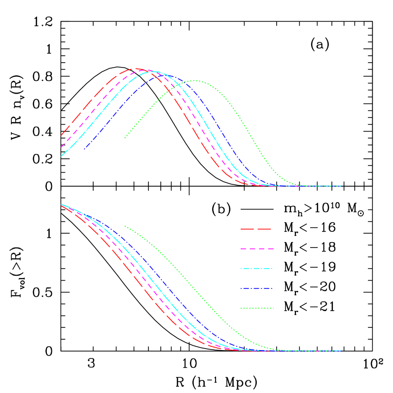
Figure 5: Abundance of voids in the excursion set formalism. All curves follow our fiducial model; they vary the minimum detectable galaxy mass as shown in the legend. Panels a and b show differential and cumulative filling factors of voids, respectively.

Figure 5 makes clear several key characteristics of the void size distribution. First, $n_{v}$ has both large and small mass cutoffs. The former occurs where $\sigma\approx\delta^{L}_{v}$, above which voids are exponentially suppressed because of the lack of large-scale power (the same mechanism that provides the large-scale cutoff in the halo mass function). The small mass cutoff occurs because of the void-crushing threshold $\delta^{L}_{p}$. The resulting characteristic scale $R_{c}$ is quite sensitive to the galaxies used to select voids: it ranges from $R_{c}\approx 5h^{-1}\mbox{ Mpc}$ for $M_{r}<-16$ to $R_{c}\approx 10h^{-1}\mbox{ Mpc}$ for $M_{r}<-21$, nearly an order of magnitude in volume. The shape, on the other hand, does not change much across the different selection thresholds. Finally, we also see that $F_{\rm vol}>1$: the voids apparently fill a volume larger than the universe. This occurs because we have let each and every void expand to its full size, even those surrounded by relatively weak overdensities just short of turnaround. These filling fractions should thus not be taken too seriously; they suggest only that, when voids are selected from galaxy surveys, we expect empty regions with $R\ga 3h^{-1}\mbox{ Mpc}$ to fill a large fraction of the universe.

The largest possible voids also provide an interesting benchmark for comparison to surveys (Blumenthal et al., 1992). To estimate $R_{\rm max}$, we find where $n_{v}=(c/H_{0})^{-3}$; i.e., the size for which we expect one void per Hubble volume. This will likely overestimate the maximum size in a real survey, because voids were smaller in the past (see §4.3 below). Of course the maximum size will also vary with the magnitude limit of the survey; for $M_{r}<(-16,\,-19,\,-21)$ we find $R_{\rm max}\approx(28,\,32,\,45)\,h^{-1}\mbox{ Mpc}$. These are compatible with existing redshift surveys; the largest voids in the 2dF survey have $R\sim 25h^{-1}\mbox{ Mpc}$ (Hoyle & Vogeley, 2004). We will make a more detailed comparison to observations in §4.5 below.

Finally, we note some simple properties of $F_{\rm vol}$. Ignoring void-crushing, the void filling fraction becomes

$$F_{\rm vol}^{\rm nc}(>R)\approx\eta^{3}\,{\rm erfc}\left[\frac{\delta^{L}_{v}(z)}{\sqrt{2}\sigma(R)}\right].$$ (13)

This is the same expression found by Dubinski et al. (1993), except that they assumed $\delta^{L}_{v}$ corresponded to shell crossing and included an extra factor of one-half (which occurred because they ignored those trajectories that joined larger voids). Void-crushing is unimportant for voids larger than the characteristic size (see §4.4 below), so equation (13) provides a reasonable estimate for $F_{\rm vol}$ and shows explicitly how it depends on $\delta^{L}_{v}$ (and hence on the survey characteristics). Dubinski et al. (1993) pointed out the interesting coincidence that $F_{\rm vol}\approx 1$ at the present day; this remains true in our model. Only recently have large voids in the faint galaxy population come to dominate the geography of the universe.

4.2 Void depth and abundance

We have seen that one key quantity in defining voids is the mean enclosed galaxy underdensity $\bar{\delta}_{\rm gal}$. Figure 6 shows how the void sizes vary with this criterion. The curves correspond to the same cases shown in Figure 2b. We see that $\bar{\delta}_{\rm gal}$ has an enormous effect on the characteristic void size $R_{c}$: it changes by a factor of three over this range of galaxy density (or a factor of nearly thirty in volume!). Moreover, in panel (b), we see that large, deep voids ($\bar{\delta}_{\rm gal}=-0.9$) only fill a small fraction of space.

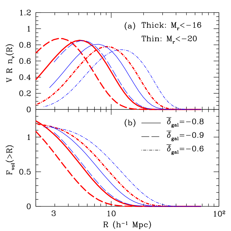
Figure 6: As Fig. 5, except we vary the mean galaxy underdensity within the voids: $\bar{\delta}_{\rm gal}=-0.8,\,-0.9$, and $-0.6$ (solid, dashed, and dot-dashed curves, respectively). The thick and thin sets of curves take $M_{r}<-16$ and $M_{r}<-20$.

4.3 Voids at higher redshifts

Just as with the halo mass function, the excursion set formalism also allows us to study how $n_{v}(m)$ evolves with redshift. We show the predicted void distribution at $z=1$ in Figure 7. In order to facilitate comparison with the $z=0$ results, we hold $m_{\rm min}$ constant between $z=1$ and the present day (as in Table 1). Of course, because the galaxy luminosity function evolves over this interval, the number density of these haloes evolves over this redshift interval.

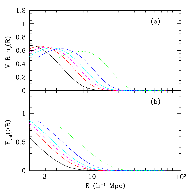
Figure 7: As Fig. 5, except for $z=1$. The galaxies are selected with the same mass thresholds as in Fig. 5 or Table 1 (with the solid curve having $m_{\rm min}>10^{10}\mbox{ M${}_{\odot}$}$ and mass increasing to the right). Note that the $z=1$ number densities differ from the $z=0$ values.

The voids also evolve, with the characteristic radius increasing significantly (by about a factor of two in each case) and the volume filling fraction also increasing (again by a factor of $\sim 2$–$3$). For example, only $\sim 10\%$ of the universe lies inside of voids with $R>10\,h^{-1}\mbox{ Mpc}$ selected from $m_{h}>1.5\times 10^{12}\mbox{ M${}_{\odot}$}$ galaxies (as opposed to $\sim 33\%$ at $z=0$). This implies that voids continue to grow, albeit relatively slowly, even after the cosmological constant dominates the energy density. Our results are in qualitative agreement with Conroy et al. (2005), who find that voids are both smaller and rarer at $z\sim 1$. A precise comparison is difficult because they use statistical techniques (specifically the void probability function) rather than identifying individual voids.

4.4 Model assumptions

Unfortunately, this model for $n_{v}(m)$ contains a number of free parameters and simplifications, so it is not nearly as well-specified as the halo mass function $n_{h}(m)$. Here we will examine how sensitive our results are to these assumptions. We begin with the halo occupation number $\left\langle N(m_{h})\right\rangle$. The solid and dashed curves in Figure 8a contrast the Kravtsov et al. (2004) value (our fiducial model) and a model with one galaxy per halo. We have previously seen that $\left\langle N\right\rangle$ only significantly affects $\delta^{L}_{v}$ if $m_{\rm min}$ is relatively small; as a result, $n_{v}(m)$ is only substantially affected for the $m_{\rm min}>10^{10}\mbox{ M${}_{\odot}$}$ survey. In this case the voids shrink by about $40\%$ in radius, with $R_{c}\sim 3h^{-1}\mbox{ Mpc}$. Thus, if we selected voids from the halo underdensity (as, for example, may be possible by associating groups of galaxies with single haloes), we would expect slightly smaller voids. The difference is minimal for bright galaxies because the mass function is steep in that regime.

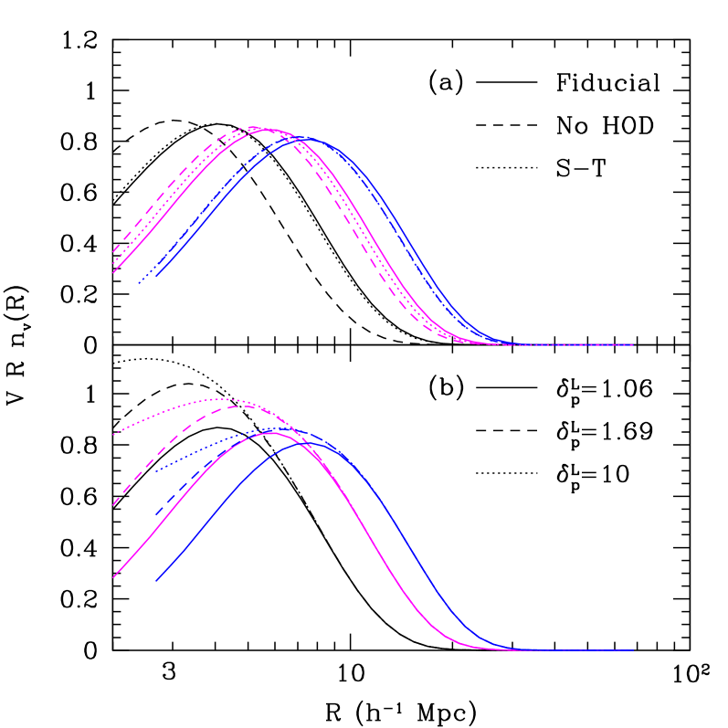
Figure 8: Void abundance for several parameter choices. All curves take our fiducial model except as noted. (a): Dashed curves assume one galaxy per dark matter halo, while the dotted curves use the Sheth-Tormen mass function (b): The solid, dashed, and dotted curves set the “void-crushing” parameter $\delta^{L}_{p}=1.06,\,1.69$, and $10$, respectively. In both panels, the three sets of curves assume surveys with $m_{\rm min}=10^{10}\mbox{ M${}_{\odot}$}$, $M_{r}<-18$, and $M_{r}<-20$, from left to right.

Figure 8a also compares the void sizes computed from the Press-Schechter mass function with those from the Sheth-Tormen mass function. To perform this comparison, we have scaled the Sheth-Tormen mass function with density in the same way as the Press-Schechter mass function (Barkana & Loeb, 2004). Thus the only real difference is the mass threshold $m_{\rm min}$, although that difference can be substantial. We see that $n_{v}(m)$ remains nearly unchanged. Thus while the void distribution may in detail depend on the exact form of $n_{h}(m)$, it is not likely to be substantially affected.

Another unknown parameter in the model is $\delta^{L}_{p}$, which describes void-crushing. Figure 8b shows its effects. Sheth & van de Weygaert (2004) argue that $\delta^{L}_{p}$ is unlikely to be smaller than $1.06$, because voids should continue to increase in size until turnaround. We therefore consider $\delta^{L}_{p}=1.69$ (where voids are only destroyed when they lie inside of collapsed haloes) and $\delta^{L}_{p}=10$ (where void crushing is negligible). This parameter clearly does have an effect on $n_{v}(m)$: ignoring void crushing dramatically increases the number of small voids. However, it has no effect on large scales, because these voids cannot be inside of extremely dense regions anyway. It also has little effect on the characteristic size $R_{c}$. Thus, while $\delta^{L}_{p}$ may affect the distribution of small voids, it is unlikely to affect the much more striking population of large voids.

Perhaps the most important simplification we have made is to ignore the scale dependence of $\delta^{L}_{v}$ so that we could use equation (10). Figure 2 shows that the threshold actually varies with the mass of the void. In principle, we should find the exact size distribution by following a procedure similar to Zhang & Hui (2005), but with two absorbing barriers. However, it is relatively easy to see that in most cases the constant barrier approximation suffices for our purposes, though more sophisticated comparisons in the future may require a more exact solution. One straightforward test is to take $\delta^{L}_{v}$ to be constant but to evaluate its amplitude at several different scales. In Figures 5–8, we have used $\delta^{L}_{v}(R=21h^{-1}\mbox{ Mpc})$. In Figure 9a, we show the corresponding distributions for the threshold evaluated at $R=70,\,7$, and $2.1h^{-1}\mbox{ Mpc}$ (solid, dashed, and dotted curves). We show results for $M_{r}<-16,\,-18$, and $-20$ (left, middle, and right sets). Clearly, for deep surveys $n_{v}(m)$ is nearly independent of the scale at which we evaluate the barrier. This is, of course, because the corresponding thresholds in Figure 2a are nearly independent of $\sigma^{2}$.

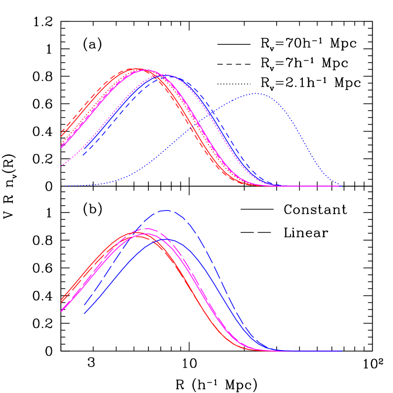
Figure 9: Void abundance for different barrier prescriptions. All curves take our fiducial model except as noted. (a): Solid, dashed, and dotted curves set the (constant) excursion set barrier by evaluating $\delta_{v}$ at $R_{v}=70,\,7$, and $2.1h^{-1}\mbox{ Mpc}$, respectively. (The fiducial model uses $R_{v}=21h^{-1}\mbox{ Mpc}$.) (b): The dashed curves use a linear fit to the excursion set barrier to compute the void abundance. In both panels, the three sets of curves assume surveys with $M_{r}<-16,\,-18$, and $-20$, from left to right.

However, if $M_{r}<-20$, the barrier rises rapidly at small scales. From Figure 9a, the distribution is still nearly independent of scale so long as $R_{v}\ga 7h^{-1}\mbox{ Mpc}$, but using $\delta^{L}_{v}(R=2.1h^{-1}\mbox{ Mpc})$ gives entirely different results. Of course, this choice is not self-consistent, because the distribution is dominated by much larger voids. To better estimate the effects of this “moving” barrier, we note that it is approximately a linear function in $\sigma^{2}$. We would therefore ideally like to solve for the mass function in the presence of a constant barrier $\delta^{L}_{p}$ and a linearly increasing barrier $\delta^{L}_{v}+\beta\sigma^{2}$. Unfortunately, we were unable to find an analytic solution for that distribution (though a straightforward numerical solution may be possible by extending Zhang & Hui 2005). We therefore instead turn to a model in which the void-crushing barrier is also linear with the same slope as the void barrier. In the Appendix, we show that the appropriate mass function is

$$n_{v}^{\ell}(m_{v})=n_{v}(m_{v})\exp(-\beta\delta^{L}_{v}-\beta^{2}\sigma^{2}/2).$$ (14)

(Note that this differs from the solution presented by Sheth & van de Weygaert 2004, which corresponds to a case with two barriers of opposite slopes; see the Appendix for a more detailed discussion.) Treating $\delta^{L}_{p}$ as a linear barrier is probably not a bad approximation. For one, the amplitude of $\delta^{L}_{p}$ does not strongly affect $n_{v}(m)$, as shown by Figure 8b. Moreover, most trajectories that cross $\delta^{L}_{v}$ would have crossed the void-crushing barrier at small $\sigma^{2}$, when $\beta\sigma^{2}\ll 1$. Finally, the appropriate choice of $\delta^{L}_{p}$ is somewhat arbitrary anyway, so a linear model may actually be more accurate.

The similarity of $n_{v}^{\ell}(m_{v})$ and $n_{v}(m)$ suggests that the linear barrier will have only a small effect on the distribution. In the cases of interest, $\beta>0$, so the first exponential factor will be larger than unity and more mass will lie inside of voids. This is intuitively obvious, because an increasing negative barrier is easier to cross. The second term affects the shape of the mass function, but it is only important for large $\beta^{2}\sigma^{2}$; in the regime we study, this factor is always smaller than unity. Figure 9b confirms these expectations. For $M_{r}<-20$, the shape remains nearly invariant (except at the smallest scales) but more mass lies inside of voids. Most importantly, the characteristic scale $R_{c}$ is nearly identical in the two cases. The linear barrier makes no difference to fainter galaxy samples, because the corresponding barrier is so nearly flat.

4.5 Comparison to observations

We are now in a position to compare our model to the observed distribution of voids. Hoyle & Vogeley (2004) compiled the most complete sample to date from the 2dF Galaxy Redshift Survey. They used the Voidfinder algorithm (El-Ad & Piran, 1997; Hoyle & Vogeley, 2002) to identify voids with $R>10\,h^{-1}\mbox{ Mpc}$ in a volume-limited sample of galaxies with $M_{b_{J}}\la-19$. They found that $\sim 35\%$ of the universe is contained inside voids with $R>10\,h^{-1}\mbox{ Mpc}$; the mean effective radius of their sample was $R\approx 15\,h^{-1}\mbox{ Mpc}$, with a maximum of $R\approx 25h^{-1}\mbox{ Mpc}$. Their algorithm separates galaxies into “wall” and “void” populations; the latter can sit inside of voids but the former are excluded. They measured a mean galaxy underdensity $\bar{\delta}_{\rm gal}=-0.93$ within voids.

With this magnitude limit, the Hoyle & Vogeley (2004) sample should find voids somewhere between the two dot-dashed curves in Figure 5 or near the thin curves in Figure 6. Given the measured $\bar{\delta}_{\rm gal}=-0.93$, the most naive comparison is to the $\bar{\delta}_{\rm gal}=-0.9$ curve in the latter, which has $F_{\rm vol}(R>10\,h^{-1}\mbox{ Mpc})\approx 16\%$ and $R_{c}\sim 5\,h^{-1}\mbox{ Mpc}$. Both of these are considerably smaller than the observed value, but it is unclear how significant the discrepancy is. Unfortunately, identifying voids at the predicted characteristic scale is difficult, because Poisson fluctuations in the galaxy distribution are substantial on Mpc scales. As a result, it is impossible to know whether an observed galaxy underdensity with $R\sim 5h^{-1}\mbox{ Mpc}$ corresponds to a true dark matter underdensity or a statistical fluctuation. Largely for this reason, Hoyle & Vogeley (2004) restrict their search to voids with $R>10\,h^{-1}\mbox{ Mpc}$. We therefore do not necessarily consider the small $R_{c}$ predicted by our model to conflict with observations; however, the discrepancy in $F_{\rm vol}$ for large voids is more worrying. We do remark that a large population of small voids have clear observational signatures, increasing the number of $\sim 5h^{-1}\mbox{ Mpc}$ empty or nearly empty regions well above those expected in a random distribution. This would manifest itself in such statistical measures as the void probability function (the probability that a region has zero galaxies; White 1979) or the underdensity probability function (the probability that a region has a given underdensity; Vogeley et al. 1989), but such statistics are (at least for the moment) beyond the capabilities of our model.

There are several more subtleties in a comparison to observations. Most importantly, the Voidfinder algorithm does not use a density threshold, so the appropriate choice of $\bar{\delta}_{\rm gal}$ is not obvious. The only “void” galaxies allowed in this approach are those that are well-isolated. But not all galaxies inside real voids need be isolated: if some fraction of the wall galaxies are actually contained inside regions with $\delta^{L}<\delta^{L}_{v}$, the true voids would be less underdense than allowed by the algorithm. Indeed, the $\bar{\delta}_{\rm gal}=-0.8$ curves in Figure 5 predict $F_{\rm vol}(R>10\,h^{-1}\mbox{ Mpc})\approx 25$–$33\%$ and $R_{c}\sim 7$–$8\,h^{-1}\mbox{ Mpc}$, much closer to the observed values. There are solid physical reasons to expect confusion between genuine void and wall galaxies. Spherical underdensities tend to evolve by evacuating their interiors, with mass accumulating in a shell near the edge (see, e.g., Dubinski et al. 1993). Gottlöber et al. (2003) showed that massive haloes pile up at the edges even more strongly. Thus it is reasonable to expect that many of the bright galaxies belonging to a large-scale underdensity lie near its edges, where they are difficult to identify unambiguously. Moreover, real surveys operate in redshift space. Because voids are expanding more rapidly than the Hubble flow, their observed volumes will be larger than the physical volumes used by our model. Goldberg & Vogeley (2004) show that the enhancement can be $\ga 20\%$ near shell-crossing.

An equally important consideration is the geometrical method used by Voidfinder to identify voids. It fills the gaps between wall galaxies with spheres and then merges overlapping spheres into discrete entities. This procedure may join two neighboring voids that our approach would consider distinct, especially if the wall between them is weak or if we include Poisson fluctuations. Galaxies on void walls tend to escape along the walls when neighboring voids merge (Dubinski et al., 1993), making this picture even more likely. Finally, voids are not uniform; rather, they are composed of a patchwork of (deeper) voids separated by weak filaments (Gottlöber et al., 2003). In the excursion set picture, this is the analog of the progenitor distribution of collapsed objects and could in principle be computed through similar techniques (Lacey & Cole, 1993), with the important difference that “sub-voids” can more easily retain their distinct identity as deeper underdensities in the galaxy distribution. The interaction of this structure with void selection algorithms is not trivial.

Another clear prediction of our model is that voids become larger as $m_{\rm min}$ increases. Hoyle & Vogeley (2004) addressed this question with statistical techniques. Specifically, they computed the void probability function and underdensity probability function for volume-limited samples with a range of magnitude thresholds (from $M_{b_{J}}<-16$ to $M_{b_{J}}<-21$). They found that both the fraction of the universe filled by voids and their characteristic size increase with the luminosity threshold, in qualitative agreement with our results. A more precise comparison requires an extension of our model to these statistics.

In summary, although our model predicts a significant population of large voids, they are still somewhat smaller than the observed structures. This could be a real discrepancy – in which case voids clearly require more sophisticated modeling – or it could be a combination of the contrasting selection techniqes, the internal void structure, and redshift-space effects. However, our qualitative conclusions (large voids, increasing in size as the underlying galaxy population brightens) do match the observed trends, a significant step forward for analytic models. Unfortunately, precise comparisons to observations will still require numerical simulations.

4.6 Comparison to simulations

Another useful comparison is to voids inside cosmological simulations. In particular, Benson et al. (2003) used the Voidfinder algorithm to identify voids inside an $N$-body simulation. They used a semi-analytic model to place galaxies within dark matter haloes and selected the voids based on the predicted properties of the galaxies. They presented the void size distributions for several different survey depths. Our results compare favorably with theirs. Like us, they found larger voids for brighter galaxies as well as larger voids for galaxies compared to the dark matter (though below $\sim 10\,h^{-1}\mbox{ Mpc}$ the two appear to converge; this may be related to the increasing importance of Poisson fluctuations). They also found that the size distribution only peaks at $R\ga 10\,\,h^{-1}\mbox{ Mpc}$ for the brightest galaxies ($M_{r}<-21.5$ and $M_{b_{J}}<-20.5$ in their models); for fainter galaxies their distributions continue rising to $R\sim 7\,h^{-1}\mbox{ Mpc}$ (below which their selection technique becomes incomplete). Finally, they find that voids typically have $\delta\approx-0.8$ and $\bar{\delta}_{\rm gal}\approx-0.9$, with both quantities decreasing rapidly toward the center of the void. The density increases sharply near, but slightly beyond, the nominal void radius. This provides a hint that the density structure may play a role in the Voidfinder selection, making direct comparisons with our predictions somewhat more difficult. Nevertheless, the good qualitative, and even reasonable quantitative, agreement of our model with these simulations provides strong support for the major features of our approach.

Colberg et al. (2005) recently examined voids in a series of large-volume $N$-body simulations. They found voids to be much smaller than our predictions, with $90\%$ of the volume contained in voids with $R<2.5\,h^{-1}\mbox{ Mpc}$. However, they selected voids based on a dark-matter density criterion $\delta_{v}<-0.8$ (corresponding to shell-crossing). This is much more restrictive than our galaxy-density criterion. The best comparison is to the $m_{h}>10^{10}\mbox{ M${}_{\odot}$}$ survey in Figure 5, whose $\delta^{L}_{v}$ is close to shell-crossing (see Fig. 2). For this sample, we find $R_{c}\approx 4h^{-1}\mbox{ Mpc}$, with much of the universe in smaller voids. The remaining discrepancy may result from the search algorithm. They began their void searches around local minima in the density field, extending them until the enclosed density exceeded $\delta_{v}$. Such a prescription may tend to find “sub-void” progenitors rather than the larger structures that correspond to the observed voids in the galaxy distribution.

5 Discussion

We have described a simple analytic model for voids in the galaxy distribution. Our model is based on Sheth & van de Weygaert (2004), who showed how to apply the excursion set formalism to underdensities. Its most important parameter is $\delta^{L}_{v}$, the linearized underdensity of a void. Those authors originally set $\delta^{L}_{v}$ to be the density corresponding to shell-crossing. However, this condition produces voids much smaller than the observed structures, whose masses can exceed those of galaxy clusters (Piran et al., 1993). Our major contribution has been to show how to define $\delta^{L}_{v}$ through the galaxy underdensity. Because galaxies are biased relative to the dark matter, voids can be nearer to the mean density than the observations naively indicate. This significantly increases the characteristic void size and the volume filling fraction.

Our model predicts voids with characteristic radii $R_{c}\sim 5$–$10h^{-1}\mbox{ Mpc}$. This is similar to, though somewhat smaller than, the voids found in galaxy redshift surveys (Hoyle & Vogeley, 2002). It is a closer match to the void population in semi-analytic galaxy formation models (Benson et al., 2003). Because bright galaxies are more highly biased, our model also predicts that voids selected from shallow surveys should be characteristically larger, in agreement with observations (Hoyle & Vogeley, 2004). However, we also predict larger galaxy densities inside voids than observed. The significance of these discrepancies is not clear: we argued in §4.5 that the algorithms used to identify voids in surveys, redshift-space distortions, and the internal structure of voids are all important in detailed comparisons to the observations. The last of these is especially crucial, because simulations show that galaxies inside voids tend to congregate near their edges (Gottlöber et al., 2003), where they are difficult to separate from genuine “wall” galaxies. Two other subtleties may also affect the comparison. The first is the nonlinear evolution of substructure within the void; we have used linear theory to describe the halo population inside voids, which likely breaks down in some regimes because power can be transferred between scales. The second is Poisson variation in the galaxy number counts (Sheth & Lemson, 1999; Casas-Miranda et al., 2002). This effect makes direct detection of small voids impossible, forcing existing surveys to search only for voids with $R\ga 10h^{-1}\mbox{ Mpc}$.

Thus it is difficult to make a precise comparison between our simple model and observed voids. However, the qualitiative agreement is reasonable. Our analytic approach is the first to contain voids with characteristic radii $\sim 10\,h^{-1}\mbox{ Mpc}$ and hence to be in even qualitative agreement with the observations. Our model shows that the enormous extent of observed voids is not particularly surprising and should not be perceived as a “crisis” for the CDM model.

By using the excursion set approach, we have also self-consistently predicted the halo population inside of voids. In agreement with naive expectations, small haloes should be less underdense than massive haloes. But the discrepancy is by no means large – typically smaller than a factor of two over three decades in halo mass. Including satellite galaxies in this calculation (which we have not done) will decrease the difference. Thus, the predicted steepening of the mass function in low-density environments is only modest and is not ruled out by existing observations of the galaxy luminosity function (Croton et al., 2005; Hoyle et al., 2005). We also emphasize that these observations determined the environmental density on relatively small scales ($\sim 8h^{-1}\mbox{ Mpc}$), where random fluctuations in the galaxy field may mimic true underdensities. If so, differences between mean and low-density environments will be further washed out. Moreover, on such scales, finite-size effects become important in setting the characteristic luminosity $L_{\star}$. The test can be sharpened by focusing on the luminosity function within large, easily identified voids – although, even there, separating void and wall galaxies may be difficult. Thus, we find no compelling reason to believe that galaxy formation differs inside and outside of voids – although we have no evidence against such a possibility, either.

Statistical properties of the galaxy distribution can also be used to test our predictions, especially for small voids that cannot be identified unambiguously. The void probability function quantifies the probability that a sphere of a given size contains no galaxies (White, 1979), and the underdensity probability function quantifies the probability that a sphere is more underdense than some specified value (Vogeley et al., 1989). These measures are free from bias in the void selection process, but they are harder to predict directly from the excursion set formalism and are less useful in identifying galaxies that reside in voids. Our model is in qualitative agreement with the observed trends in these statistics (Hoyle & Vogeley, 2004; Conroy et al., 2005), but more work is needed to connect our formalism to them.

Appendix A The First Crossing Distribution for Two Barriers

Sheth & van de Weygaert (2004) showed how to derive equation (10) using the Laplace transform. Here we present an alternate derivation (similar to McQuinn et al. 2005) and generalize it to the case of two linear barriers with equal slope. We begin by considering two constant barriers $\delta^{L}_{p}=B_{p}$ and $\delta^{L}_{v}=B_{v}$. The distribution of trajectories $Q(\delta^{L},S)$, where $S=\sigma^{2}$, obeys the diffusion equation

$$\frac{\partial Q}{\partial S}=\frac{1}{2}\,\frac{\partial^{2}Q}{\partial(\delta^{L})^{2}}.$$ (15)

The appropriate boundary conditions are $Q(B_{p},S)=Q(B_{v},S)=0$ and $Q(\delta^{L},0)=\delta_{D}(\delta^{L})$, where $\delta_{D}$ is the Dirac delta function. We first make the simple transformation $y=\delta^{L}-B_{v}$. We then assume $Q(y,S)=f(S)g(y)$; equation (15) becomes

$$\frac{1}{f}\,\frac{{\rm d}f}{{\rm d}S}=\frac{1}{2g}\,\frac{{\rm d}^{2}g}{{\rm d}y^{2}}=-\alpha^{2},$$ (16)

where $\alpha$ is a constant. The general solutions are $f(S)=\exp(-\alpha^{2}S)$ and $g(y)=\exp(-\sqrt{2}\alpha y)$. The boundary conditions $g(0)=g(B_{p}-B_{v})=0$ select the sine function for the latter and force its argument to take discrete values; thus

$$Q(y,S)=\sum_{n=1}^{\infty}a_{n}\,\sin\left(\frac{n\pi y}{B_{p}-B_{v}}\right)\,\exp\left[-\frac{n^{2}\pi^{2}S}{2(B_{p}-B_{v})^{2}}\right].$$ (17)

We fix the constants $a_{n}$ by matching to the function $Q(y,0)=\delta_{D}(y+B_{v})$. Thus

$$Q(y,S) = \sum_{n=1}^{\infty}\frac{2\,\sin(n\pi D)}{B_{p}-B_{v}}\,\sin\left(\frac{n\pi y}{B_{p}-B_{v}}\right)$$ (18)

$$\times\exp\left[-\frac{n^{2}\pi^{2}S}{2(B_{p}-B_{v})^{2}}\right],$$

where $D\equiv-B_{v}/(B_{p}-B_{v})$. The total rate at which trajectories disappear from the permitted region is

$$-\frac{\partial}{\partial S}\int_{0}^{B_{p}-B_{v}}{\rm d}y\,Q(y,S)=-\frac{1}{2}\left[\frac{\partial Q}{\partial y}\right]_{0}^{B_{p}-B_{v}},$$ (19)

where we have used equation (15). We interpret the two terms on the right hand side as the rate at which trajectories flow across the two barriers. Thus the first-crossing distribution for the void barrier is

$$F_{v}(S) = \frac{1}{2}\,\left.\frac{\partial Q}{\partial y}\right|_{y=0}$$ (20)

$$= \sum_{n=1}^{\infty}\frac{(n\pi D)^{2}}{B_{v}^{2}}\,\frac{\sin(n\pi D)}{n\pi}\,\exp\left[-\frac{n^{2}\pi^{2}D^{2}}{2B_{v}^{2}/S}\right],$$

which yields equation (10) after converting to mass units.

We now consider the case of two absorbing barriers linear in $S$, $\delta^{L}_{p}=B_{p}+B_{1}S$ and $\delta^{L}_{v}=B_{v}+B_{1}S$. We make the coordinate transformation $u=B_{1}(\delta^{L}-B_{1}S)-B_{1}B_{v}$; then the boundary conditions on $u$ become $Q(0,S)=0$ and $Q(u_{1},S)=0$, where $u_{1}\equiv B_{1}(B_{p}-B_{v})$. The boundary condition on $S$ becomes

$$Q(u,0)=\delta_{D}(\delta^{L})=B_{1}\,\delta_{D}(u+B_{1}B_{v})\,\exp(-u-B_{1}B_{v}).$$ (21)

The diffusion equation (15) becomes

$$\frac{\partial Q}{\partial S}=\frac{B_{1}^{2}}{2}\left(\frac{\partial^{2}Q}{\partial u^{2}}+2\frac{\partial Q}{\partial u}\right).$$ (22)

We again assume a separable solution $Q(u,S)=f(S)g(u)$. The general solutions are exponentials, and the boundary conditions on $g$ select the sine function with discrete arguments. Thus the solution is again a Fourier sine series in $u$. The Fourier coefficients $a_{n}$ can be fixed by matching the solution to equation (21). We then find that

$$Q(u,S) = e^{-u}\,\sum_{n=1}^{\infty}\frac{2\sin(n\pi D)}{B_{p}-B_{v}}\,\sin\left[\frac{n\pi u}{B_{1}(B_{p}-B_{v})}\right]\,$$ (23)

$$\times\exp\left[-B_{1}B_{v}-\frac{B_{1}^{2}S}{2}-\frac{n^{2}\pi^{2}S}{2(B_{p}-B_{v})^{2}}\right];$$

note the similarity to equation (18). The rate at which trajectories cross the barriers is

$$-\frac{\partial}{\partial S}\int_{0}^{u_{1}}{\rm d}\delta^{L}Q(\delta^{L},S)=-\frac{B_{1}}{2}\left[\frac{\partial Q}{\partial u}\right]_{0}^{u_{1}}-B_{1}[Q]_{0}^{u_{1}}.$$ (24)

But $Q(0,S)=Q(u_{1},S)=0$; thus we can again identify the first-crossing distribution of the linear void barrier $F_{v}^{\ell}$ with the $u=0$ component of the first part, so

$$F_{v}^{\ell}(S) = \frac{B_{1}}{2}\left.\frac{\partial Q}{\partial u}\right|_{0}$$ (25)

$$= F_{v}(S)\,\exp(-B_{1}B_{v}-B_{1}^{2}S/2),$$

from which the mass function follows directly. Note that this expression differs from equation (C10) of Sheth & van de Weygaert (2004). Those authors tried to derive the same distribution through Laplace transforms. Their solution required the first-crossing distribution of $\delta^{L}_{p}$ and $\delta^{L}_{v}$ to be identical (their equation C6); this is not the case if the barriers have equal slope $B_{1}$, because then they are not symmetric about the $\delta^{L}=0$ axis. Instead their solution applies to a case in which the slopes of the two barriers have opposite signs.

References

- Barkana & Loeb (2004) Barkana R., Loeb A., 2004, ApJ, 609, 474
- Benson et al. (2003) Benson A. J., Hoyle F., Torres F., Vogeley M. S., 2003, MNRAS, 340, 160
- Bertschinger (1985) Bertschinger E., 1985, ApJS, 58, 1
- Blanton et al. (2003) Blanton M. R., et al., 2003, ApJ, 592, 819
- Blumenthal et al. (1992) Blumenthal G. R., da Costa L. N., Goldwirth D. S., Lecar M., Piran T., 1992, ApJ, 388, 234
- Bond et al. (1991) Bond J. R., Cole S., Efstathiou G., Kaiser N., 1991, ApJ, 379, 440
- Casas-Miranda et al. (2002) Casas-Miranda R., Mo H. J., Sheth R. K., Boerner G., 2002, MNRAS, 333, 730
- Cen (2005) Cen R., 2005, submitted to ApJ (astro-ph/0507014)
- Colberg et al. (2005) Colberg J. M., Sheth R. K., Diaferio A., Gao L., Yoshida N., 2005, MNRAS, 360, 216
- Cole & Kaiser (1989) Cole S., Kaiser N., 1989, MNRAS, 237, 1127
- Conroy et al. (2005) Conroy C., et al., 2005, submitted to ApJ (astro-ph/0508250)
- Cooray (2005) Cooray A., 2005, submitted to MNRAS (astro-ph/0505421)
- Croton et al. (2005) Croton D. J., et al., 2005, MNRAS, 356, 1155
- de Lapparent et al. (1986) de Lapparent V., Geller M. J., Huchra J. P., 1986, ApJ, 302, L1
- Dubinski et al. (1993) Dubinski J., da Costa L. N., Goldwirth D. S., Lecar M., Piran T., 1993, ApJ, 410, 458
- Einasto et al. (1989) Einasto J., Einasto M., Gramann M., 1989, MNRAS, 238, 155
- Efstathiou et al. (1988) Efstathiou G., & Frenk C. S., & White S. D. M., & Davis M., 1988, MNRAS, 235, 715
- El-Ad & Piran (1997) El-Ad H., Piran T., 1997, ApJ, 491, 421
- El-Ad & Piran (2000) El-Ad H., Piran T., 2000, MNRAS, 313, 553
- El-Ad et al. (1997) El-Ad H., Piran T., Dacosta L. N., 1997, MNRAS, 287, 790
- Fillmore & Goldreich (1984) Fillmore J. A., Goldreich P., 1984, ApJ, 281, 9
- Friedmann & Piran (2001) Friedmann Y., Piran T., 2001, ApJ, 548, 1
- Furlanetto et al. (2005) Furlanetto S. R., McQuinn M., Hernquist L., 2005, MNRAS, in press (astro-ph/0507524)
- Goldberg et al. (2005) Goldberg D. M., Jones T. D., Hoyle F., Rojas R. R., Vogeley M. S., Blanton M. R., 2005, ApJ, 621, 643
- Goldberg & Vogeley (2004) Goldberg D. M., Vogeley M. S., 2004, ApJ, 605, 1
- Gottlöber et al. (2003) Gottlöber S., Łokas E. L., Klypin A., Hoffman Y., 2003, MNRAS, 344, 715
- Gregory & Thompson (1978) Gregory S. A., Thompson L. A., 1978, ApJ, 222, 784
- Heath (1977) Heath D. J., 1977, MNRAS, 179, 351
- Hoyle et al. (2005) Hoyle F., Rojas R. R., Vogeley M. S., Brinkmann J., 2005, ApJ, 620, 618
- Hoyle & Vogeley (2002) Hoyle F., Vogeley M. S., 2002, ApJ, 566, 641
- Hoyle & Vogeley (2004) Hoyle F., Vogeley M. S., 2004, ApJ, 607, 751
- Jenkins et al. (2001) Jenkins A., Frenk C. S., White S. D. M., Colberg J. M., Cole S., Evrard A. E., Couchman H. M. P., Yoshida N., 2001, MNRAS, 321, 372
- Kirshner et al. (1981) Kirshner R. P., Oemler A., Schechter P. L., Shectman S. A., 1981, ApJ, 248, L57
- Kravtsov et al. (2004) Kravtsov A. V., Berlind A. A., Wechsler R. H., Klypin A. A., Gottlöber S., Allgood B., Primack J. R., 2004, ApJ, 609, 35
- Lacey & Cole (1993) Lacey C., Cole S., 1993, MNRAS, 262, 627
- Mo & White (1996) Mo H. White S. D. M., 1993, MNRAS, 282, 347
- Müller et al. (2000) Müller V., Arbabi-Bidgoli S., Einasto J., Tucker D., 2000, MNRAS, 318, 280
- Mathis & White (2002) Mathis H., White S. D. M., 2002, MNRAS, 337, 1193
- McQuinn et al. (2005) McQuinn M., Furlanetto S. R., Hernquist L., Zahn O., Zaldarriaga M., 2005, ApJ, in press (astro-ph/0504189)
- Peebles (1980) Peebles P. J. E., 1980, The Large-Scale Structure of the Universe. Princeton: Princeton University Press
- Peebles (2001) Peebles P. J. E., 2001, ApJ, 557, 495
- Piran et al. (1993) Piran T., Lecar M., Goldwirth D. S., da Costa L. N., Blumenthal G. R., 1993, MNRAS, 265, 681
- Press & Schechter (1974) Press W. H., Schechter P., 1974, ApJ, 187, 425
- Sheth & Lemson (1999) Sheth R. K., Lemson G., 1999, MNRAS, 304, 767
- Sheth & Tormen (1999) Sheth R. K., Tormen G., 1999, MNRAS, 308, 119
- Sheth & Tormen (2002) Sheth R. K., Tormen G., 2002, MNRAS, 329, 61