Molecular cloud evolution. I. Molecular cloud and thin CNM sheet formation

Abstract

We analyze the scenario of molecular cloud formation by large-scale supersonic compressions in the diffuse warm neutral medium (WNM). During the early stages of this process, a shocked layer forms, and within it, a thin cold layer. An analytical model and high-resolution 1D simulations predict the thermodynamic conditions in the cold layer. After $\sim 1$ Myr of evolution, the layer has column density $\sim 2.5\times 10^{19}{\rm~{}cm}^{-2}$, thickness $\sim 0.03$ pc, temperature $\sim 25$ K and pressure $\sim 6650$ K ${\rm~{}cm}^{-3}$. These conditions are strongly reminiscent of those recently reported by Heiles and coworkers for cold neutral medium sheets. In the 1D simulations, the inflows into the sheets produce line profiles with a central line of width $\sim 0.5{\rm~{}km~{}s}^{-1}$ and broad wings of width $\sim 1{\rm~{}km~{}s}^{-1}$. Being the result of the inflows rather than of turbulence, these linewidths do not imply excessively short lifetimes for the sheets. At later times, 3D numerical simulations show that the cold layer undergoes a dynamical instability that causes it to develop turbulent motions and to increase its thickness, until it becomes a fully three-dimensional turbulent cloud. The destabilization mechanism appears to be the nonlinear thin shell instability, triggered by the thermal instability-induced density contrast. In the simulations, fully developed turbulence arises on times ranging from $\sim 7.5$ Myr for inflow Mach number $M_{\rm 1,r}=2.4$ to $>80$ Myr for $M_{\rm 1,r}=1.03$. Due to the limitations of the simulations, these numbers should be considered upper limits. In the turbulent regime, the highest-density gas (HDG, $n>100{\rm~{}cm}^{-3}$) is always overpressured with respect to the mean WNM pressure by factors 1.5–4, even though we do not include self-gravity. The intermediate-density gas (IDG, $10<n[{\rm cm}^{-3}]<100$) has a significant pressure scatter that increases with $M_{\rm 1,r}$, so that at $M_{\rm 1,r}=2.4$, a significant fraction of the IDG is at a higher pressure than the HDG. The ratio of internal to kinetic energy density varies from the inflow to the IDG and the HDG, and increases with density in the most turbulent runs. Our results suggest that the turbulence and at least part of the excess pressure in molecular clouds can be generated by the compressive process that forms the clouds themselves, and that thin CNM sheets may be formed transiently by this mechanism, when the compressions are only weakly supersonic.

1 Introduction

Molecular cloud complexes (or “giant molecular clouds”, GMCs) are some of the most studied objects in the interstellar medium (ISM) of the Galaxy. Yet, their formation mechanism and the origin of their physical conditions remain uncertain (see, e.g., Elmegreen, 1991; Blitz & Williams, 1999). In particular, GMCs are known to have masses much larger than their thermal Jeans masses (Zuckerman & Palmer, 1974, sec. 7.2) (i.e., thermal energies much smaller than their absolute gravitational energy), but comparable gravitational, magnetic, and turbulent kinetic energies (Larson, 1981; Myers & Goodman, 1988; Crutcher, 1999, 2004; Bourke et al., 2001). This similarity has traditionally been interpreted as indicative of approximate virial equilibrium, and of rough stability and longevity of the clouds (see, e.g., McKee et al., 1993; Blitz & Williams, 1999). In this picture, the fact that molecular clouds have thermal pressures exceeding that of the general ISM by roughly one order of magnitude (Blitz, 1991; Mac Low & Klessen, 2004) is interpreted as a consequence of the fact that they are strongly self-gravitating. Because of their self-gravitating and overpressured nature, molecular clouds were left off global ISM models based on thermal pressure equilibrium, such as those by Field, Goldsmith & Habing (1969) and McKee & Ostriker (1977).

Recent work suggests instead that molecular clouds and their substructure may actually be transient features in their respective environments. In this picture, the clouds and their substructure are undergoing secular dynamical evolution, being assembled by large-scale supersonic compressions in the atomic medium on a crossing time and becoming self-gravitating in the process (Elmegreen, 1993, 2000; Vázquez-Semadeni, Passot & Pouquet, 1996; Ballesteros-Paredes, Vázquez-Semadeni & Scalo, 1999; Ballesteros-Paredes, Hartmann & Vázquez-Semadeni, 1999; Hartmann, Ballesteros-Paredes & Bergin, 2001; Pringle, Allen & Lubow, 2001; Hartmann, 2003; Bergin et al., 2004; Vázquez-Semadeni et al., 2005). Specifically, Hartmann, Ballesteros-Paredes & Bergin (2001) suggested that the accumulation process of atomic gas may last a few tens of megayears until the gas finally becomes molecular, self-gravitating and supercritical at roughly the same time (see also Franco & Cox, 1986). Observations of atomic inflows surrounding molecular gas support this scenario (Ballesteros-Paredes, Hartmann & Vázquez-Semadeni, 1999; Brunt, 2003).

In this scenario, the excess pressure in molecular clouds may arise from the fact that they have been assembled by motions whose ram pressures are comparable or larger than the local thermal pressure, so that both the excess pressure and the self-gravitating nature of the clouds may originate from the compression that forms the cloud, and need not be an indication of any sort of equilibrium (Maloney, 1990; Ballesteros-Paredes & Vázquez-Semadeni, 1997; Ballesteros-Paredes, Vázquez-Semadeni & Scalo, 1999; Clark et al., 2005). Additionally, it has been suggested by Vázquez-Semadeni, Ballesteros-Paredes & Klessen (2003a) that a substantial fraction of the internal turbulence of the clouds may originate from thin-shell instabilities in the compressed gas, rather than from local energy injection from the clouds’ own stellar products (see also Hartmann, Ballesteros-Paredes & Bergin, 2001). This would explain the fact that even clouds with no apparent stellar content (see, e.g., Maddalena & Thaddeus, 1985) have levels of turbulence comparable to clouds with healthy star-forming activity.

Since the typical velocity dispersion in the warm medium (which we will denote generically as WNM, as we will not distinguish between neutral and ionized warm components) is $\sim 10$ km s^-1 (Kulkarni & Heiles, 1987; Heiles & Troland, 2003), the flow is transonic (i.e., with rms Mach number $\sim 1$). Under these conditions, transonic compressions in the WNM may render the gas unstable to two main types of instabilities. On one hand, there is the thermal instability (TI), originally studied by Field (1965) (see also the reviews by Meerson, 1996; Vázquez-Semadeni et al., 2003b), and by McCray, Stein & Kafatos (1975) in the context of radiative post-shock cooling regions, in which it causes the formation of thin cold sheets parallel to the shock front. The formation of cold neutral medium (CNM) structures induced by compressions in the WNM has been more recently studied analytically and numerically by Hennebelle & Pérault (1999, 2000) and Audit & Hennebelle (2005).

On the other hand, there are bending mode instabilities, which cause rippling of the compressed layer, and, eventually, fully developed turbulence. The nonlinear theory was laid down by Vishniac (1994) in the isothermal case, who referred to the instability as nonlinear thin-shell instability (NTSI), a name which we use throughout this paper. More recently, Pittard et al. (2005) have studied the stability of cooling shocks and its dependence on the Mach number and the final post-shock temperature, finding that lower final temperatures cause greater overstability. Numerically, several groups have studied the problem in a variety of contexts, such as the interiors of molecular clouds at sub-pc scales (Hunter et al., 1986), stellar wind interactions (Stevens et al., 1992), cloud collisions (Klein & Woods, 1998), and in a general fashion (Walder & Folini, 1998, 2000). In particular, the simulations of the latter authors show that turbulence is generated and maintained for the entire duration of the inflowing motions.

In the context of the thermally bistable atomic medium, a two-dimensional study of converging flows in the diffuse atomic medium has been recently presented by Audit & Hennebelle (2005), but focusing on the competition between externally imposed turbulence and the tendency of TI to produce two-phase structure, rather than in the production of turbulence by the process. In a related context, Koyama & Inutsuka (2002) and Inutsuka & Koyama (2004) have studied the production of supersonic turbulence behind a propagating shock wave in the warm neutral ISM, showing that cold, dense cloudlets are formed, with bulk velocities that are supersonic with respect to their internal temperatures, proposing this mechanism as the origin of molecular cloud turbulence. However, these authors attributed the development of turbulence to TI alone without indicating the precise mechanism at play, and focused on the structure behind a single traveling shock wave, rather than on the structure in shocked compressed layers between converging flows. Instead, large molecular masses typical of GMCs probably require focused, large-scale compressive motions that may last several tens of megayears, as in the scenario proposed by Hartmann, Ballesteros-Paredes & Bergin (2001). In this case, the turbulence generation might last for as long as the accumulation (compression) lasts, and the turbulence in molecular clouds could be considered as driven, rather than decaying. A preliminary study of the development of the turbulence in these circumstances has been recently presented by Heitsch et al. (2005), who also investigated the masses and possible self-gravitating nature of the clumps formed by the induced turbulence.

The advanced stages of molecular cloud evolution are also poorly understood. Traditionally, the greatest concern about molecular clouds has been how to support them against self-gravity, and it was speculated that turbulence could be prevented from decaying if it consisted primarily of MHD waves (Arons & Max, 1975), although numerical work strongly suggests that MHD turbulence decays just as fast as hydrodynamic turbulence (Mac Low et al., 1998; Stone, Ostriker & Gammie, 1998; Mac Low, 1999; Padoan & Nordlund, 1999; Lazarian & Beresnyak, 2005). Clouds were assumed to be finally dispersed by the kinetic energy injection from their stellar products (e.g., Elmegreen, 1991, sec. 5)

Instead, in the secular-evolution scenario cloud support may not be a concern at all. Clouds start as atomic entities with negligible self-gravity that increase their mean density as they are compressed, so that their self-gravity also increases in the process. When they finally become strongly self-gravitating, collapse does occur, albeit in a localized fashion that involves a small fraction of the total cloud mass, due to the action of their internal turbulence, which forms nonlinear density fluctuations that may collapse themselves on times much shorter than the parent cloud’s free-fall time (Sasao, 1973; Elmegreen, 1993; Padoan, 1995; Vázquez-Semadeni, Passot & Pouquet, 1996; Ballesteros-Paredes, Vázquez-Semadeni & Scalo, 1999; Klessen, Heitsch & Mac Low, 2000; Heitsch, Mac Low & Klessen, 2001; Padoan & Nordlund, 2002; Li et al., 2004; Li & Nakamura, 2004; Nakamura & Li, 2005; Vázquez-Semadeni et al., 2005; Clark & Bonnell, 2005). The mass that does not collapse sees its density reduced, and may possibly be dispersed as soon as the external compression ends. Indeed, even in simulations of decaying, non-magnetic self-gravitating turbulence, the star formation efficiency is smaller than unity (e.g., Bate, Bonnell & Bromm, 2003), and some of the cloud’s mass is dispersed away from the simulation box (Clark & Bonnell, 2004; Clark et al., 2005).

The present paper is the first in a series that analyzes quantitatively the turbulent scenario of molecular cloud evolution, assuming that they are formed by large-scale compressions in the warm diffuse medium. Here we focus on the formation stages, investigating the physical conditions that may be produced in the compressed layer as a function of the Mach number of the converging streams, and so we neglect the chemistry and self-gravity of the gas and use moderate-resolution simulations to test the order-of-magnitude estimates that can be made from simple considerations, the triggering of thin-shell instabilities, and the statistics of the physical conditions in the turbulent gas.

We also report on the formation of transient, thin sheets of cold gas during the initial stages of the cloud formation process. These sheets turn out to closely match the properties of cold neutral medium (CNM) sheets recently observed by Heiles and collaborators (Heiles & Troland, 2003; Heiles, 2004). These authors have reported on the existence of extremely thin CNM sheets, with thicknesses $\sim 0.05$ pc, column densities, $\sim 0.2\times 10^{20}{\rm~{}cm}^{-2}$, temperatures $\sim 20$ K and linewidths $\sim 1~{}{\rm~{}km~{}s}^{-1}$, and have argued that these properties are difficult to understand in terms of turbulent clouds. We will argue that objects with these properties are naturally formed as part of the cloud formation process, in cases of low-Mach number compressions.

The plan of the paper is as follows: In §2 we describe the basic physics of the pre-turbulent stages of the system, and then in §3 we present numerical simulations that confirm the estimates and follow the nonlinear stages in which the compressed and cooled layers become turbulent. We describe the numerical method in §3.1, relevant resolution considerations in §3.2, and the results in §3.3. In §4 we discuss our results, comparing them with observational data and previous work. Finally, in 5 we give a summary and some conclusions.

2 The physical system

2.1 Governing equations

We consider the atomic medium in the ISM, whose flow and thermal conditions are governed by the equations

$$\frac{\partial\rho}{\partial t}+\nabla\cdot(\rho{\bf v})=0$$ (1)

$$\frac{\partial(\rho{\bf v})}{\partial t}+\nabla\cdot(\rho{\bf v}{\bf v})=-\nabla P$$ (2)

$$\frac{\partial E}{\partial t}+\nabla\cdot\left[(E+P){\bf v}\right]=\rho\left(\Gamma-\rho\Lambda(T)\right),$$ (3)

where $\rho$ is the gas density, v is the fluid velocity, $E=P/(\gamma-1)+\rho|{\bf v}|^{2}/2$ is the total energy per unit volume, $P$ is the thermal pressure, $e=P/[\rho(\gamma-1)]$ is the internal energy per unit mass $T=e/c_{\rm V}$ is the temperature, $c_{\rm V}=[\gamma(\gamma-1)]^{-1}$ is the specific heat at constant volume, $\gamma=5/3$ is the heat capacity ratio of the gas, $\Gamma$ is the heating rate, and $\rho\Lambda$ is the radiative cooling rate. We use a piecewise power-law fit to the cooling function, based on a fit to the standard thermal-equilibrium (TE) pressure versus density curve of Wolfire et al. (1995), as decribed in Sánchez-Salcedo, Vázquez-Semadeni & Gazol (2002) and Gazol, Vázquez-Semadeni & Kim (2005). The fit is given by

$$\Lambda(T)=\left\{\begin{array}[]{ll}0&\mbox{$T<15\>K$}\\ 3.42\times 10^{16}T^{2.13}&\mbox{$15\>K\leq T<141\>K$}\\ 9.10\times 10^{18}T&\mbox{$141\>K\leq T<313\>K$}\\ 1.11\times 10^{20}T^{0.565}&\mbox{$313\>K\leq T<6101\>K$}\\ 2.00\times 10^{8}T^{3.67}&\mbox{$6101\>K\leq T$.}\end{array}\right\}$$ (4)

The background heating is taken as a constant $\Gamma=2.51\times 10^{-26}{\rm erg}\;{\rm s}^{-1}{\rm H}^{-1}$, where “H^-1” means “per Hydrogen atom”. This value is roughly within half an order of magnitude of the value of the dominant heating mechanism (photo-electric heating) reported by Wolfire et al. (1995) throughout the range $10^{-2}{\rm cm}^{-3}\leq n\leq 10^{3}{\rm cm}^{-3}$. Note that we have for now neglected magnetic fields, self-gravity, and heating and cooling processes adequate for the molecular regime.

The condition of thermal equilibrium between heating and cooling at a given density defines TE-values of the temperature and thermal pressure, which we denote by $T_{\rm eq}(\rho)$ and $P_{\rm eq}(\rho)$. Figure 1 shows $P_{\rm eq}$ versus number density $n$ for the cooling and heating functions defined above. As is well known (Field, Goldsmith & Habing, 1969), at the mean midplane thermal pressure of the ISM ($\sim 2250$ K cm^-3 or sightly higher, Jenkins & Tripp, 2001), the atomic medium is thermally bistable. For our chosen fits to the cooling and heating functions, and a mean pressure of $2400$ K${\rm~{}cm}^{-3}$, a warm diffuse phase ($n_{1}\sim 0.35$ cm^-3, $T\sim 7400$ K) is able to coexist in pressure equilibrium with a cold dense one ($n_{2}\sim 37$ cm^-3, $T\sim 65$ K). A third, unstable phase with ($n_{3}\sim 1$ cm^-3, $T\sim 2400$ K) also corresponds to the same equilibrium pressure, but is not expected to exist under equilibrium conditions because it is unstable. The equilibrium values of the density are also shown in fig. 1. Due to our neglect of molecular-phase cooling and heating, our $P_{\rm eq}$-$n$ curve does not correctly represent the approximately isothermal behavior of molecular gas above densities of a few hundred cm^-3, and so we introduce a slight error in the thermodynamic conditions of the densest gas. We expect to address this shortcoming in subsequent papers, which will also take into account the chemistry in the gas and the transition to the molecular phase.

2.2 Problem description and physical discussion

2.2.1 Analytical model of the early stages

Within the warm medium described above, we consider the collision of two oppositely-directed gas streams with speeds comparable to the sound speed, since the velocity dispersion in the warm ISM is known to be roughly sonic (e.g. Kulkarni & Heiles, 1987; Heiles & Troland, 2003). This compressive motion may have a variety of origins (the passage of a spiral density wave, or a large-scale gravitational instability, or general transonic turbulence in the diffuse medium), whose details are not of our concern here. The discussion below on the early evolution of the system is inspired by that of Hennebelle & Pérault (1999), except that in our case we assume that the inflows are maintained in time rather than being impulsive, and that our simulations are three-dimensional.

The colliding streams have the density and thermal pressure conditions of the warm diffuse phase, forming a shock-bounded slab at the collision site, as illustrated in fig. 2. During the initial stages the evolution is adiabatic, the bounding shocks move outwards from the collision site, and the gas inside the shocked slab is heated and driven away from thermal equilibrium by the shocks. The gas in the slab then has conditions dictated by the adiabatic jump relations (see, e.g., Shu, 1992). For later use, we transcribe here the jump conditions for the velocity and the pressure:

$$u_{2} = \left(\frac{\gamma-1+\frac{2}{M_{1}^{2}}}{\gamma+1}\right)u_{1},$$ (5)

$$P_{2} = \left(\frac{1-\gamma+2\gamma M_{1}^{2}}{\gamma+1}\right)P_{1},$$ (6)

where the subindex “1” denotes the pre-shock (or upstream) quantities, subindex “2” denotes quantities immediately downstream of the shock, and the symbol $u$ denotes velocities in the frame of reference of the shock. Velocities in the rest frame are denoted by the symbol $v$.

Denoting by $v_{\rm s}$ the shock speed (in the rest frame) one has

$$u_{2}=v_{2}-v_{\rm s}$$ (7)

and

$$u_{1}=v_{1}-v_{\rm s}.$$ (8)

At the time of the shock formation, the velocity $v_{2}$ is simply zero and it is thus possible to calculate the initial shock speed by combining eqs. (5), (7) and (8). One obtains the following quadratic equation for $v_{\rm s}$ as a function of $v_{1}$

$$2v_{\rm s}^{2}-v_{\rm s}v_{1}(3-\gamma)-\left[v_{1}^{2}(\gamma-1)+2c_{1}^{2}\right]=0,$$ (9)

where $c_{1}=\gamma P_{1}/\rho_{1}$ is the sound speed in the (warm diffuse) pre-shock medium. The solution of this equation, expressed in terms of the inflow Mach number in the rest frame $M_{\rm 1,r}\equiv v_{1}/c_{1}$, is

$$\frac{v_{\rm s}}{c_{1}}=\frac{-M_{\rm 1,r}(\gamma-3)\pm\sqrt{{M_{\rm 1,r}}^{2}\left[(\gamma-3)^{2}+8(\gamma-1)\right]+16}}{4}.$$ (10)

As time progresses, the gas in the slab begins to cool significantly, so that most of the internal energy increase caused by the shock is radiated away after roughly a cooling time, which we take here as

$$\tau_{\rm c}\equiv\frac{c_{\rm V}T_{2}}{\rho\Lambda(\rho_{2},T_{2})-\Gamma},$$ (11)

where $\Lambda(\rho_{2},T_{2})$ is the cooling function evaluated at the immediate post-shock conditions. Equation (11) is well defined in the shock-heated, out-of-TE post-shock gas, in which $\rho\Lambda(\rho_{2},T_{2})>\Gamma$.

At $t\sim\tau_{\rm c}$, the flow returns close to its local equilibrium temperature. If the adiabatic-jump value of the immediate post-shock pressure is higher than the maximum TE pressure allowed for the warm gas, then the cooling brings the gas to the cold branch of the TE curve, creating a thin, dense, cold layer in the middle of the compressed slab (McCray, Stein & Kafatos, 1975, see also Hennebelle & Pérault 1999). We interchangeably refer to this dense layer as the “cold” or the “condensed” layer, and to its boundary as the condensation front. The strong cooling undergone by the gas as it flows into the central regions causes the thermal pressure to drop to values comparable to that of the inflow, the density to increase, and the outer shock to decelerate. TI exacerbates this process by creating such a large density contrast ($>100$) between the inflow and the central layers that a quasi-stationary situation is reached in which shocked layer thickness becomes almost constant and the outer shock is almost at rest. For $t\gtrsim\tau_{\rm c}$, the cold slab has a half-thickness of roughly one cooling length $l_{\rm c}$, given by $l_{\rm c}\approx v_{2}\tau_{\rm c}$, and the velocity field across the shocked layer takes values between $v_{2}$ (immediately behind the shock) and zero at the center of the cold slab.

The cooling time ($\tau_{\rm c}$) and length ($l_{\rm c}$) as functions of the inflow Mach number are plotted in fig. 3. As we will discuss in §3.1, the cooling length constitutes the minimum physical size that the numerical box must have.

The pressure in the central cold layer can be estimated assuming that the total pressure, sum of the kinetic and ram pressures, is constant in the shocked region. The immediate post-shock pressures and velocities are given by the jump conditions, eqs. (5) and (6), using an upstream velocity equal to the inflow speed, since at this time the shock is not moving in the rest frame. The central pressure $P_{3}$ (in what follows, we denote quantities in the condensed layer by the subindex “3”) is thus estimated as

$$P_{3}=P_{2}+\rho_{2}v_{2}^{2}$$ (12)

since the velocity is zero at the center of the condensed layer.

The density in the condensed layer can then be estimated from the fact that its constituent gas has undergone a phase transition from the warm to the cold phase, in which the approach to TE is extremely fast. This means that the density in the cold layer is given by the thermal-equilibrium value at $P_{3}$. For a power-law cooling function $\Lambda\propto T^{\beta}$ and a constant heating function, it can be shown that the equilibrium pressure satisfies $P_{\rm eq}\propto\rho^{\gamma_{\rm e}}$, with $\gamma_{\rm e}=1-1/\beta$ being an effective polytropic exponent (see, e.g., Vázquez-Semadeni, Passot & Pouquet, 1996). Thus, the dense branch of our $P_{\rm eq}$ vs. $\rho$ curve, in which $\beta=2.13$, is described by the equation

$$P_{\rm eq}=350\left(\frac{n}{{\rm 1~{}cm^{-3}}}\right)^{0.53}{\rm K~{}cm}^{-3}.$$ (13)

Setting $P_{\rm eq}=P_{3}$ in the above equation and inverting to solve for the density, we obtain the dependence of the cold layer density $n_{3}$ on the inflow Mach number $M_{\rm 1,r}$, shown as the solid line in fig. 4. Note that for molecular gas the density is not expected to increase as rapidly with $M_{\rm 1,r}$, because in this case the flow is approximately isothermal so that $\gamma_{\rm e}\sim 1$ (Scalo et al., 1998; Spaans & Silk, 2000).

If the problem were strictly one-dimensional, then the condensed layer would simply thicken in time, with its bounding front moving at a speed $v_{\rm f}\approx(n_{2}/n_{3})v_{2}$, an estimate based on mass conservation from the immediate post-shock region to the cold slab.

This velocity is shown as the dotted line in fig. 4. We see that, somewhat counterintuitively, the front speed decreases with increasing $M_{\rm 1,r}$. This is because the density contrast between the condensed layer and its surroundings increases rapidly with $M_{\rm 1,r}$, and thus the mass entering the condensed layer is compacted very efficiently, causing a very mild increase in the slab thickness. Finally, the dash-dotted line in fig. 4 gives the pressure in the condensed layer.

The column density through the slab increases with time and is given by $N_{3}=2n_{3}v_{\rm f}\Delta t$, where $\Delta t$ is the time since the beginning of the condensation process, and the factor of 2 comes from the fact that $v_{\rm f}\Delta t$ is the half-thickness of the cold layer. The dashed line in fig. 4 shows the column density through the slab after 1 Myr in units of $10^{16}$ cm^-2, as a function of $M_{\rm 1,r}$. We see that the column density in the cold layer varies relatively slowly with $M_{\rm 1,r}$, with values $2\times 10^{19}$–$10^{20}$ cm^-2 at $\Delta t=1$ Myr.

The simple model given in this section then predicts the values of the physical variables in the cold layer. In §3.3.1 we compare its predictions with the results of 1D high-resolution numerical simulations of the process.

2.2.2 Late stages

The description of the late stages of the evolution requires numerical simulations, which we present in §3. Here we just give some general discussion and expectations.

Shock compressed layers are known to be nonlinearly unstable in the isothermal case (Vishniac, 1994), meaning that large enough inflow Mach numbers are needed to trigger the instability. Specifically, displacements of the compressed layer comparable to its thickness are necessary to trigger the instability. This would seem to create a difficulty for destabilizing the compressed layers in the WNM, given the transonic nature of the flow.

However, cooling apparently helps in bringing down the threshold for instability, as suggested by the recent results of Pittard et al. (2005). These authors found that there exists a critical value $\beta_{\rm cr}$ of the cooling exponent for the appearance of the well-known global overstability in radiative shocks (Langer, Chanmugam & Shaviv, 1981), and that this exponent depends on both the upstream Mach number and the ratio $\chi$ of the cold layer temperature to the pre-shock temperature. The relevant result for our purposes is that low-Mach number, low-$\chi$ shocks have values of $\beta_{\rm cr}$ that are comparable to those of high-Mach number shocks with high $\chi$. That is, lower cold-layer temperatures bring down the required Mach number for overstability. Since the temperature ratio between the cold and warm phases in the atomic medium is $\chi\sim 0.01$, the compressed layers formed by transonic compressions in this medium can probably become overstable, producing oscillations that can bend the layer strongly enough to trigger a nonlinear thin shell-like (NTS-like) instability even at relatively low Mach numbers. Indeed, in the simulations reported in §3, we have always found that the compressed layer eventually becomes unstable, given enough time and resolution. We have found no threshold for suppression of the NTS-like instability in the range of inflow Mach numbers we have explored.

3 Numerical simulations

In this section we present moderate-resolution simulations that are intended mostly as an exploratory tool of parameter space and of the phenomena described in the previous section. Detailed, high-resolution simulations using adaptive-mesh and smoothed-particle hydrodynamics techniques will be presented in future papers to investigate the details of the small-scale gasesous structures as well as the star formation that result in this scenario.

3.1 Numerical method and limitations

We solve the hydrodynamic equations together with the energy conservation equations using Eulerian hydrodynamics code based on the total variation diminishing (TVD) scheme (Ryu et al., 1993). It is a second-order accurate upwind scheme, which conserves mass, momentum and energy. We include the heating and cooling functions described in §2.1 as source terms after the hydrodynamic step. Tests have shown that this procedure is accurate enough, so that we did not have to implement an“operator splitting” algorithm (where the execution of the hydrodynamic and source stages is alternated) which formally preserves the second order accuracy.

We solve the equations both in one (1D) and three (3D) dimensions. The 1D runs are used for testing the analytical model of §2.2.1. The 3D runs, in which the inflows enter along the $x$ direction, use periodic boundary conditions along the $y$ and $z$ directions and the same resolution in all three directions (200 grid cells), except for two runs that use a lower resolution (50 grid cells) in the $z$ direction and open boundary conditions in $y$ and $z$, that we used at early stages of this work for studying the dependence of the time for turbulence development on the $x$ and $y$ resolution.

In the 3D runs, a random component in time and space, of amplitude $0.5v_{0}$, is added to the inflow speed at each cell of the boundary as a generic way of triggering the dynamical instabilities of the compressed layer without the biasing that might be introduced if we used, for example, fluctuations with a pre-defined power spectrum. Being so fast and small-scale, most of this component is erased by diffusivity, so that the velocity inside the box fluctuates only by a few percent.

No explicit term for heat conduction is included. In the ideal, absolutely non-conducting case, the fastest-growing mode of TI has a vanishing length scale (Field, 1965). Numerically, this would imply instability at the scale of the grid size, producing numerical instabilities. In the presence of thermal conductivity, the smallest unstable length scale (the “Field length”) is finite (Field, 1965), and sensitively dependent on the local temperature. If the Field length is not resolved, numerical diffusion still stabilizes the smallest available scales, producing a “numerical Field length” larger than the real one (Gazol, Vázquez-Semadeni & Kim, 2005), even if explicit heat conduction is not included, and in this case the scale of the fastest-growing mode is resolution-dependent (Koyama & Inutsuka, 2004). In practice, this means that if the resolution is insufficient, the size of the structures formed by TI is not adequately resolved and determined. However, in the presence of turbulence, in which large-scale supersonic motions are the main drivers of density fluctuations rather than the development of TI, the statistics of the dense gas (pressure and density distributions), which will be our main focus in this paper, are rather insensitive to the resolution even in simulations without thermal conduction (Gazol, Vázquez-Semadeni & Kim, 2005). We conclude that, in spite of not including thermal conduction explicitly, the moderate resolution we have used should cause an overestimate of the sizes of the structures (“clumps”) formed, but should have no serious effect on the density and pressure statistics of the dense gas we discuss below.

Aware of the above limitations, we adopt the following convenient set of units for the simulations: $n_{0}=1$ cm^-3, $T_{0}=10^{4}$ K, $v_{0}=c_{0}=11.74$ km s^-1, where $c_{0}$ is the adiabatic sound speed at $T_{0}$. All simulations start with inflows at $T=7100$ K and $n=0.338$ cm^-3, which correspond to the equilibrium warm phase at a pressure $P=2400$ K cm^-3. The inflow’s velocity, given in terms of its Mach number with respect to its sound speed of 9.89 km s^-1, is varied between $M=1.03$ to $M=2.4$.

The physical size of the box deserves some special discussion. In §2.2.1 we have noted that during the very early stages of the system’s evolution, the shocks move outwards, stopping after roughly one cooling time, and having traversed one cooling length. In order to capture the full dynamics of the problem, we must make sure that the box has a large enough physical size that the shocks do not leave the simulation before stopping. We have found that actual cooling lengths are larger by factors of $\sim 4$ than indicated by fig. 3. Moreover, at late stages of the evolution, the slab becomes heavily distorted and thickens considerably (see also, e.g., Walder & Folini, 2000). So we use box sizes significantly larger than the cooling length given in fig. 3. As seen in this figure, the cooling length is a rapidly decreasing function of the inflow Mach number $M_{\rm 1,r}$ in the range we have considered, and so simulations with smaller $M_{\rm 1,r}$ require larger box lengths. Finally, the physical box size implies a physical time unit given by $t_{0}=L_{0}/v_{0}$,

We take as a fiducial simulation one with $M_{\rm 1,r}=2.4$ and a box length $L_{0}=16$ pc. The coefficients of the cooling function for the fiducial case in code units are 561.641 for 15 K $\leq T<141$ K, 4.6178 for 141 K $\leq T<313$ K, 1.0244 for 313 K $\leq 6101$ K, and 4.7432 for $T>6101$ K. Other box sizes (and derived time units) are obtained by simply multiplying the cooling and heating coefficients by the same factor as that for the box size, because the only simulation parameter on which the cooling rates depend is the time unit. Table 1 summarizes the main parameters of the runs we consider below, in which the runs are denoted mnemonically by their inflow Mach number $M_{\rm 1,r}$ and their box size $L_{0}$ as Mn.nLnn, where ’n’ is an integer. We denote 1D runs by the suffix “1D”, high-resolution versions of another run by the suffix “hr”, and simulations with lower resolution in the $z$ direction, by the suffix “LZ”, for “low-$z$”.

3.2 Resolution considerations

Before we discuss the results of the numerical simulations, it is important to discuss the resolution limitations of the simulations we present here and their effects, in order to be able to usefully interpret their results. The cold layer is estimated to be very thin, $\sim 2v_{\rm f}\Delta t=0.029$ pc for $M_{\rm 1,r}=1$, for which $v_{\rm f}=0.014{\rm~{}km~{}s}^{-1}$, when taking $\Delta t=1$ Myr. Moreover, we have seen (fig. 4) that the front speed $v_{\rm f}$ is a decreasing function of $M_{\rm 1,r}$, and therefore the cold layer is thinner for higher $M_{\rm 1,r}$. This means that only run M1.03L64-1Dhr should barely resolve (with $\sim 2$ grid cells) the cold layer at this time. In practice the layer is not quite resolved even at this time, since apparently at least 8–9 zones are necessary to resolve the layer (see below). This implies that the thickness of the cold layer during the early, non-turbulent stages depends on the resolution, and is exaggerated, in some cases grossly, by our simulations. Figure 5 shows profiles along the $x$-axis at half the $y$ and $z$ extensions of the $x$-velocity (solid line), density (dash-dotted line), temperature (dahed line) and pressure (dotted line) for runs M1.03L64-1D (left panel) and M1.03L64-1D-hr (right panel) at $t=5.33$ Myr. These runs differ only in the resolution used. It is clear that the cold layer is thinner in the high-resolution case.

The fact that the cold layer thickness is initially resolution-limited also implies that the density within it is artificially reduced, since the layer is thicker than it should, and the total mass in the layer is determined only by the accretion rate, which is independent of the resolution. In turn, this implies that the pressure is below its physical value, as clearly seen in fig. 5. The pressure in the cold layer can only reach the equilibrium value with its surroundings at later times when the slab thickness is enough for the density to reach its physical value. This happens at times $\sim$ 16.0 and 8.0 Myr for runs M1.03L64-1D and M1.03L64-1D-hr, respectively, at which the slab can be considered to start being well resolved. This condition is shown in fig. 6, in which the peak density is seen to have converged in the two runs at different times.

However, since the total mass in the layer is independent of the resolution, we expect a similar situation for the layer’s column density. Indeed, the thickness of the slab in run M1.03L64-1D at $t=5.33$ Myr (fig. 5) is $\sim 9$ grid zones, or $\sim 0.58$ pc, with a maximum density of $\sim 99.7$ cm^-3. The column density through the layer is measured at $N\approx 7.6\times 10^{19}$ cm^-2. This can be compared with the estimates of §2.2.1. For $M_{\rm 1,r}=1$, the model gives $v_{\rm f}=0.014$ km s^-1 and $n_{3}=240$ cm^-3, so that after $\Delta t=5.33$ Myr, the layer thickness should be $\ell=2v_{\rm f}\Delta t\approx 0.15$ pc, and the column density $N\approx 1.125\times 10^{20}{\rm~{}cm}^{-2}$. Thus, the column density in the simulation is within a $\sim 30$% error of the predicted value, even though the layer is $\sim 3.9$ times thicker than predicted at this time. For run M1.03L64-1D-hr, the slab thickness is $\sim 15$ zones, or $\sim 0.24$ pc, and the maximum density is $218$ cm^-3, so the layer is close to being well resolved, but not quite yet. The measured column density is $N\approx 6.8\times 10^{19}$, within a $\sim 40$% error of the predicted value. The column densities measured in the simulations at this early time are lower than the predicted value at this time because the layers in the simulations have actually bell-shaped profiles, rather than the flat ones that develop at later times, at which the agreement with the model predictions is much better (see §3.3.1 and fig. 8).

From the above discussion we conclude that the resolution of the simulations in this paper is generally insufficient for correctly resolving the structure inside the cold layer during the initial stages of the evolution. Nevertheless, the column density of the cold layer is reasonably recovered even from the early stages of the simulations.

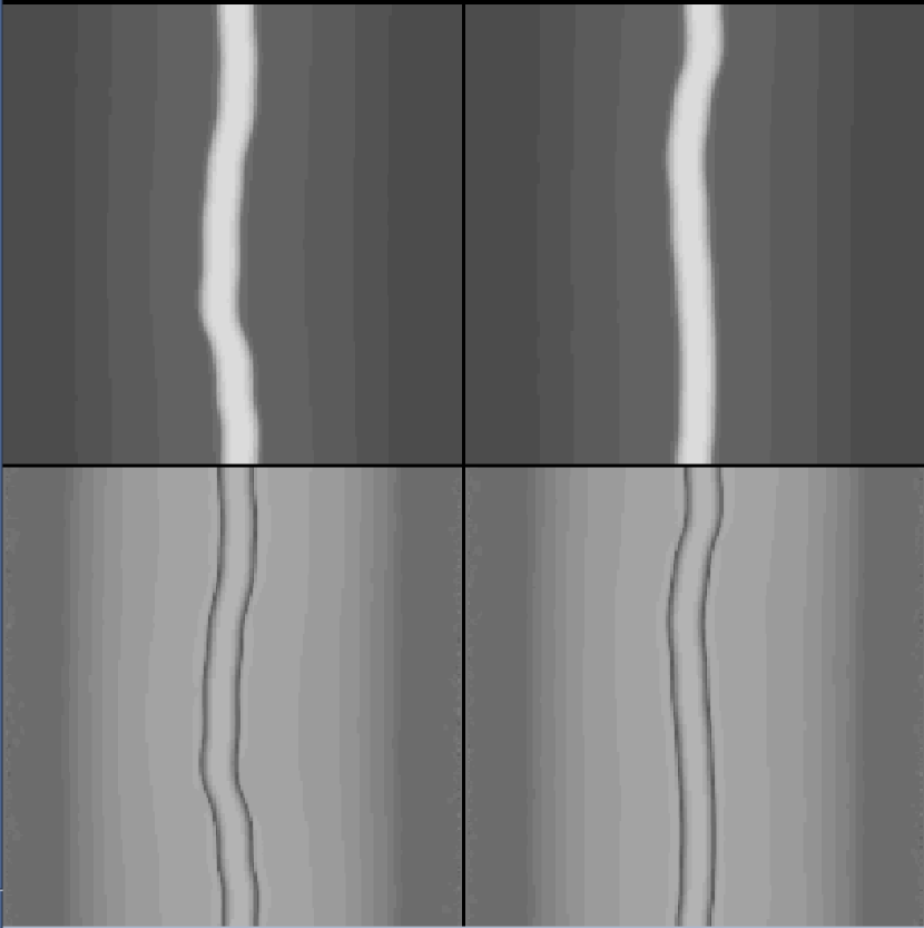
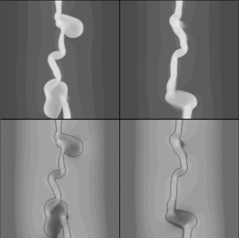
Figure 7: Cross-section views of the density (upper rows) and the pressure (lower rows) at $z=25$ (left columns) and at $z=50$ (right columns) of runs M1.03L64 (left) and M1.03L64hr (right) at $t=106.6$ Myr. The density and pressure ranges are $(\rho_{\rm min},\rho_{\rm max})=(0.34,223){\rm~{}cm}^{-3}$, $(P_{\rm min},P_{\rm max})=(1800,6200)$ K ${\rm~{}cm}^{-3}$ for run M1.03L64 and $(\rho_{\rm min},\rho_{\rm max})=(0.34,370){\rm~{}cm}^{-3}$, $(P_{\rm min},P_{\rm max})=(1190,8100)$ K ${\rm~{}cm}^{-3}$ for run M1.03L64hr. The higher-resolution run has already started to develop turbulence, while the lower-resolution one is only undergoing slab bending at this time.)

With respect to the late stages of the evolution, we have found empirically that as the resolution is increased, the instability in the compressed layer develops earlier. This is shown in fig. 7, which depicts constant-$z$ slices of the density (upper panels) and of the pressure (lower panels) for runs M1.03L64-LZ (left) and M1.03L64-hr-LZ (right) at the last computed step ($t=106$ Myr). It is seen that the instability has already developed in the high-resolution run, but not quite yet in the low-resolution one, although in this run the cold layer is already significantly bent, and presumably turbulence will be generated soon after this time. Since our 3D simulations are still far from resolving the true Field length in the various ISM regimes, the effect of numerical diffusion roughly approaches that of the correct heat conduction as the resolution is increased. Therefore, the observed trend of decreasing turbulence development time with increasing resolution implies that the timescales reported in this paper should be considered upper limits only.

Concerning the structures formed by the turbulence in the compressed layer, once it has developed fully, the main limitation introduced by the limited resolution is that the size of the cold structures will be artificially bounded from below by the numerical cell size, but we expect no other serious limitation. The structures are mainly formed by the turbulent flow, not by TI, and therefore they can in principle form with a variety of sizes, rather than at the characteristic scales of the TI, which indeed are very small.

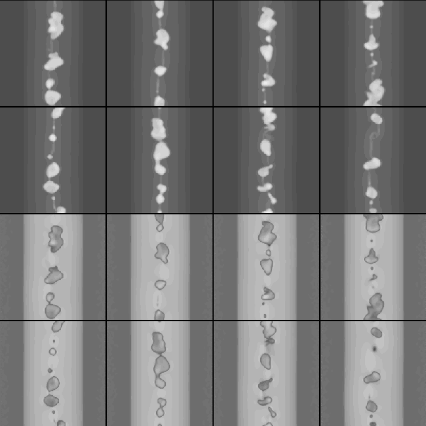
Figure 11: Cross-section views at eight $z$ values, spaced by $\Delta z=25$ grid cells, of the density (upper two rows) and pressure (lower two rows) in run M1.2L32 at $t=20$ Myr. The dynamic ranges of the density and pressure are indicated by the left panels of figs. 13 and 14, respectively. The still image in the printed version corresponds to frame 15 in the animation available in the electronic edition of the Astrophysical Journal. In the animation, the density and pressure frames are reversed.

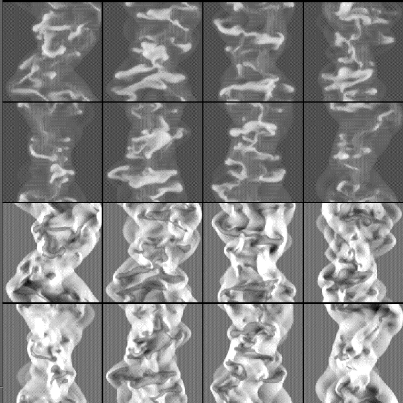
Figure 12: Same as fig. 11 but for run M2.4L16. The dynamic ranges of the density and pressure are indicated by the right panels of figs. 13 and 14, respectively.

Finally, we note that, as seen from figs. 11 and 12, in runs M1.2L32 and M2.4L16, as the turbulent layer thickens, its bounding shock eventually touches the inflow boundary. This happens at times $t=42.6$ Myr for run M1.2L32 (frame 32 in the corresponding animation, fig. 11, with the frame-count starting at frame zero), and $t=7.34$ Myr for run M2.4L16 (frame 11 in fig. 12). At this point, the simulations are in principle not valid anymore, as the interaction of the material in the turbulent layer with the inflowing gas ceases to be followed in full. In practice, however, we have found that the statistical properties of the simulation are not affected by the collision of the shock with the boundary. This fact can be understood because the inflow boundary conditions effectively act as outflow conditions for the material reaching the boundary from the inside of the box, and so effectively this gas just leaves the box as through standard outflow conditions, while fresh gas continues to flow in through these boundaries, and to interact with the gas remaining in the simulation. Thus, in §3.3.3 we discuss various physical and statistical properties both at the time the shocks leave the simulations, and at the time when the statistics become stationary.

3.3 Results

3.3.1 Comparison with the analytical model

The predictions of the analytical model of §2.2.1 can be compared with the results of the 1D numerical simulations, which resolve the layer at not-too-late times, and in which the slab does not become unstable. To be consistent with the hypotheses of the model, we consider times late enough that the outer shock has essentially stopped.

As illustrations, we discuss the cases with $M_{\rm 1,r}=1.03$ and 1.2. The left panel of fig. 8 shows the density field in the central 6 pc of run M1.03L64-1Dhr at times 26.6 Myr and 79.8 Myr. We can see that the right-hand side of the dense cold layer has moved 0.8 pc, from $x=32.3$ pc to $x=33.1$ pc. This gives a velocity $v_{\rm f}=0.015{\rm~{}km~{}s}^{-1}$. We also read the density inside the layer as 255${\rm~{}cm}^{-3}$. The right panel of fig. 8 shows the pressure throughout the entire simulation at $t=26.6$ Myr. The maximum value of the pressure, occurring at the center of the dense layer, is $P_{3}=6653$ K${\rm~{}cm}^{-3}$. This can be compared with the model predictions for $M_{\rm 1,r}=1.03$, which are $P_{3}=6643$ K${\rm~{}cm}^{-3}$, $n_{3}=257{\rm~{}cm}^{-3}$ and $v_{\rm f}=0.014{\rm~{}km~{}s}^{-1}$, in excellent agreement with the measurements.

Figure 9 shows the corresponding comparison in the case $M_{\rm 1,r}=1.2$. In this case, the left panel shows that the front moves from $x=16.20$ pc at $t=13.3$ Myr to $x=16.65$ pc at $t=53.2$ Myr, implying $v_{\rm f}=0.011{\rm~{}km~{}s}^{-1}$. We also read a cold layer density of $n_{3}=338{\rm~{}cm}^{-3}$. In turn, the right panel shows the pressure, whose maximum value is $P_{3}=7734$. For a Mach number $M_{\rm 1,r}=1.2$, our model gives $P_{3}=8160$ K${\rm~{}cm}^{-3}$, $v_{\rm f}=0.0106{\rm~{}km~{}s}^{-1}$ and $n_{3}=378{\rm~{}cm}^{-3}$ (cf. fig. 4). This is again in good agreement with the results of the simulation.

We conclude that the analytical model and the 1D numerical simulations are consistent with each other, giving us confidence in both, and confirming the physical scenario (an outer shock front and an inner condensation front), in which thin sheets form during the initial stages of the compression.

3.3.2 Global evolution

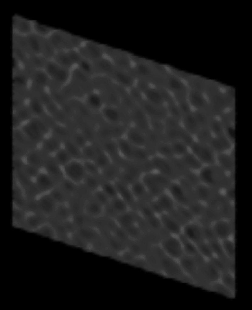
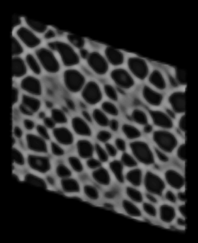
Figure 10: Projection views of the density field in run M1.03L64 at $t=5.33$ Myr (left, corresponding to frame 2 in the animation of the entire evolution available in the electronic edition of the Astrophysical Journal, with the frame-count starting at zero) and at $t=10.67$ Myr (right, frame 4). The thin sheet is seen to fragment into a honeycomb pattern.

In this section we now discuss the evolution of the compressed and the cold layers in runs with various inflow Mach numbers. In the animations of figures 10, 11 and 12 we respectively show the evolution of runs M1.03L64, M1.2L32 and M2.4L16. The spacing between frames in the animations is $\Delta t=0.5$ code time units (cf. Table 1 for the time unit in each run), which corresponds to $\Delta t=$ 2.66, 1.33 and 0.66 Myr, respectively. The animations in figures 11 and 12 show constant-$z$ cross-sections of the simulation at different, equally-spaced $z$ values, with $\Delta z=25$ grid cells, to illustrate the evolution of the thickness and structure of the dense “layer” (which, in the late stages, becomes a turbulent cloud). The animation in fig. 10 shows instead a transluscent projection of the density evolution in run M1.03L64, to illustrate the fragmentation process of the thin dense layer. The still figures of the printed version show selected panels from the animations to also illustrate these features.

From the animations and figures, several points are noticed. In general, we see that, after the formation of the thin cold layer, the latter begins to fragment into a filamentary honeycomb pattern, with denser clumps at the sites where the filaments intersect. Subsequently, the density structures begin to move on the plane of the dense layer, merging and forming larger clumps. However, apparently the random fluctuations in the inflow velocity cause the merging clumps to collide with slight offsets, which therefore cause the layer to thicken and to develop vorticity. Ultimately, the motion in the cold thin layer appears to completely destabilize the entire thick shocked slab, and fully developed turbulence ensues.

In fig. 11 it is interesting to note that the density peaks (“clouds”) appear surrounded by a low-pressure interface in the pressure images. This region probably corresponds in our simulations to a numerical effect, with the pressure gradient being compensated there by numerical diffusion, although in real clouds this may correspond to a conducting interface. This interface, however, is not apparent in the pressure images for run M2.4L16 (fig. 12). These results suggest that sharp phase transitions between the warm and cold gas still exist at $M_{\rm 1,r}=1.2$ (Audit & Hennebelle, 2005), but tend to be erased at $M_{\rm 1,r}=2.4$, as also suggested by the pressure histograms discussed in §3.3.3. Nevertheless, even in run M1.2L32, the pressure in the “clouds” is seen to fluctuate significantly, because of their dynamical origin, and in general they are not all at the same pressure nor at uniform pressure inside.

An important datum of the simulations is the time they require for attaining a saturated turbulent state. This can be defined in practice as the timescale for reaching a stationary shape of the statistical indicators, such as the density and pressure histograms. We find that this occurs at $t\approx 47.9$ Myr for run M1.2L32 (frame 36 in the corresponding animation, fig. 11), and at $t\approx 10.7$ Myr for run M2.4L16 (frame 11 in fig. 12). Run M1.03L64 does not seem to have reached a stationary state by the end of the integration time we have considered, $t=80.1$ Myr. As mentioned in §3.2, these times are larger than those at which the shocks reach the boundary, and therefore in the next section we discuss both.

3.3.3 Properties of the turbulent state

Density and pressure distributions

In this section we concentrate on the cases with $M_{\rm 1,r}=1.2$ and $M_{\rm 1,r}=2.4$, as they are the ones in which significant amounts of turbulence can develop within realistic timescales in the shocked layer. Figure 13a shows the density histograms of run M1.2L32 at $t=42.6$ Myr (solid line, frame 32 in the animation of fig. 11), when the shock touches the boundary, and at $t=47.9$ Myr, when the statistics become stationary (dotted line, frame 36 in the animation). The histograms at the two times are very similar, although the former one contains slightly lower numbers of grid cells with intermediate- and high-densities, indicative of the not yet completely stationary turbulent regime at that time. Similarly, fig. 13b shows the density histograms at the corresponding times for run M2.4L16 ($t=7.37$ Myr, frame 11, solid line, and $t=10.7$ Myr, frame 16, dotted line). The same trends are observed for this run.

The histograms of both runs have narrow and tall peaks at the density of the unperturbed inflowing streams (the density of the warm phase, $n_{1}=0.34~{}{\rm~{}cm}^{-3}$). The histogram of the mildly supersonic run M1.2L32 is significantly bimodal, although it extends to densities $\sim 400$ cm^-3, well into what is normally associated with typical molecular cloud densities. The peak of the high-density maximum of the distribution is between $\sim 50$ and $100~{}{\rm~{}cm}^{-3}$. In contrast, the histogram for the strongly supersonic run M2.4L16 has a less pronounced bimodal character, and extends at roughly constant height to densities typical of the cold phase, to then start decreasing at higher densities, to reach values close to 1000 cm^-3. Thus, a higher inflow Mach number tends to erase the signature of bistability of the flow by increasing its level of turbulence, in agreement with the studies by Sánchez-Salcedo, Vázquez-Semadeni & Gazol (2002), Audit & Hennebelle (2005) and Gazol, Vázquez-Semadeni & Kim (2005).

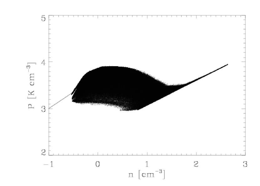
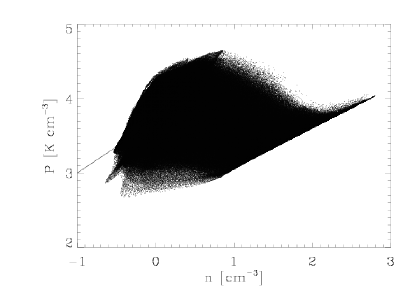
Figure 15: Pressure-versus-density plots of runs M1.2L32 at $t=42.6$ Myr (left) and of run M2.4L16 at $t=7.37$ Myr (right). The solid lines show the locus of the equilibrium pressure as a function of density.

Of particular interest is the pressure distribution in these simulations, as a means to understanding the overpressured nature of molecular clouds. Figures 14a and b show the pressure histograms of runs M1.2L32 (at $t=42.6$ Myr) and run M2.4L16 (at $t=7.37$ Myr). Shown are the histograms for the entire simulation (dotted lines), for gas with densities 10 cm${}^{-3}<n<100$ cm^-3 (dashed lines), which we will refer to as the “intermediate-density” gas (IDG), and for gas with densities $n>100$ cm^-3 (solid lines), which we will refer to as “high-density” gas (HDG). The histograms for all components are normalized to the total number of points. We will generally identify the IDG with the CNM, although we do not use this nomenclature because in some cases the IDG is highly pressurized, and thus warm rather than cold. On the other hand, the HDG can be identified with the “molecular” component, although we will maintain the notation HDG because we do not follow the chemistry nor have cooling appropriate for the molecular gas. The times shown for figs. 14a and b are the same as the eralier times in figures 13a and b. Figures 15a and b in turn show the distribution of points in the simulations in the $(P,\rho)$ plane, overlayed on the $P_{\rm eq}$ vs. $\rho$ curve, at the same times as fig. 14.

Several points are worth noting in these figures. First, again the pressure of the unperturbed inflow gas is noticeable as the sharp peak at $\log P=3.38$ ($P=2400$ K cm^-3) in the pressure histograms of the entire simulations. However, the global shape of the two histograms is very different. The total histogram for run M1.2L32 (fig. 14a) is quite narrow, with a total width of slightly over one order of magnitude, and moreover has a second, wide maximum centered at $P\sim 5000$ K cm^-3. Instead, the total pressure histogram of run M2.4L16 (fig. 14b) extends over two orders of magnitude and has a nearly lognormal shape (except for the sharp peak noted above), rather than the bimodal shape of the $M_{\rm 1,r}=1.2$ run. All of this indicates a more developed state of the turbulence in run M2.4L16.

Focusing on the pressure distributions for the IDG and HDG, we note that, in run M1.2L32, the pressure in the IDG is mostly confined to lower values than those of the HDG, in the range 1000–4000 K cm^-3, with a very low tail extending to $\sim 7000$ K${\rm~{}cm}^{-3}$. The most probable value of the pressure of this gas practically coincides with that of the unperturbed inflowing WNM, with $P\sim 2400$ K cm^-3. The HDG, on the other hand, is systematically overpressured with respect to the IDG and the unperturbed WNM, with $4000\lesssim P/({\rm K~{}cm}^{-3})\lesssim$ 10,000. It is interesting that the broad high-pressure maximum in the total histogram overlaps with the range of pressure values of the “molecular” gas. This maximum corresponds to the shocked, low-density gas that is in transit from the warm to the cold phases, crossing the unstable density range, $0.6\lesssim n\lesssim 7{\rm~{}cm}^{-3}$, as can be seen in fig. 15a. The pressure coincidence between the HDG and the shocked unstable gas strongly suggests that the HDG is in pressure balance with the shocked, compressed gas, rather than with the ambient WNM, explaining its higher-than-average pressure.

In the case of run M2.4L16, some new features arise. Most notably, the pressure distribution of the WNM and the IDG now extend beyond that of the HDG (see also fig. 15b). This is somewhat surprising, and probably indicates that a substantial fraction of the pressure in the shocked gas is converted into kinetic energy of the HDG by the dynamical instabilities, rather than into internal energy. This picture is supported by the fact discussed in the next subsection, that the ratio of turbulent kinetic-to-internal energy density is highest in the HDG in this high-$M_{\rm 1,r}$ run. It is also interesting that the pressure distribution of the HDG extends over a very similar range ($4000\lesssim P/({\rm K~{}cm}^{-3})\lesssim 10000$) as that of the mildly supersonic case M1.2L32, in spite of the much higher pressures present in the IDG and WNM distributions.

Energy densities and rms speeds in the various regimes

Table 2 summarizes the energy densities of the inflowing WNM, the IDG and the HDG for the two runs under consideration. For the IDG and the HDG, the table additionally gives the rms speed, rms Mach number, and mean temperature. The data for each run are given at two times: the time at which the shocks first touch the $x$-boundaries, and the (later) time at which the density and pressure histograms become stationary (cf. §3.3.2). We see that the statistics for the IDG indiceate that indeed it is slightly more turbulent at the later times for both runs, with larger velocity dispersions, rms Mach numbers and lower mean temperatures (indicating larger densities due to stronger compressions). The statistics for the HDG, however, are nearly indistinguishable at the two times.

Note that the velocity statistics reported in Table 2 refer to the total velocity dispersion of these components, and thus includes the bulk motions of the moving dense gas parcels. Although we have not measured it here, it has consistently been reported by various groups (Koyama & Inutsuka, 2002; Heitsch et al., 2005) that the internal velocity dispersion of the dense gas regions is subsonic. We do not attempt these measurments here, and defer the task for future papers using higher resolution simulations.

It can be seen from Table 2 that in run M1.2L32 both the IDG and the HDG have higher internal than kinetic energy densities. The opposite is true for run M2.4L16, in which the kinetic energy density in these two components is 2.5–3.5 times larger than the internal energy density. Note in fact that the kinetic energy density in the turbulent IDG and HDG is larger than that in the inflowing streams. This does not constitute any violation of energy conservation, since the volume occupied by the IDG and the HDG is small compared with that of the diffuse WNM.

Finally, from the rms speed and Mach number data for the IDG and HDG in the two runs we see that their motions are in general transonic (in the IDG) or supersonic (in the HDG) with respect to their own sound speeds. The rms Mach number in the HDG is lower than typical values for molecular clouds, but this can be attributed mainly to the relatively low resolution of the simulations, causing the velocities and the density fluctuations to be somewhat damped at the scales of the dense gas by numerical diffusion. This causes lower velocities and higher temperatures, thus lowering the Mach number. Moreover, we do not model the transition from atomic to molecular hydrogen, so that the simulations do not account for the reduction of the sound speed upon the formation of molecules. But we see that the velocity dispersion, $\sim 1.7~{}{\rm~{}km~{}s}^{-1}$ would correspond to Mach numbers $\sim 8.5$ in molecular gas at $T\sim 10$ K.

4 Discussion and comparison with previous work

4.1 CNM sheet formation at early stages

Our results from both the qualitative analysis and the numerical simulations show that during the early stages of evolution, the collision of WNM streams may form thin sheets of CNM, whose properties are described in §§2.2.1 and 3.3.1 and fig. 4. Since the sheets last the longest at low inflow Mach numbers, we consider the results of simulation M1.03L64-1Dhr, reported in §3.3.1.

According to this simulation, the outward velocity of the cold layer boundary is $v_{\rm s}\sim 0.015$ km s^-1, implying that the layer thickness is

$$\ell=0.0306\left[\frac{t}{1{\rm~{}Myr}}\right]{\rm~{}pc},$$ (14)

and, with a number density $n_{3}\sim 255{\rm~{}cm}^{-3}$, its column density is

$$N_{3}=2.4\times 10^{19}\left[\frac{t}{1{\rm~{}Myr}}\right]{\rm~{}cm}^{-2}.$$ (15)

The pressure in the cold layer is $P_{3}=6650$ K ${\rm~{}cm}^{-3}$, and therefore its temperature is $T\approx 26$ K. These values are interestingly similar to those derived by Heiles & Troland (2003, hereafter HT03) (see also Heiles, 2004) for cloud “A” of Knapp & Verschuur (1972), of $N\sim 0.2\times 10^{20}{\rm~{}cm}^{-2}$, $T\sim 20$ K, $n\sim 150{\rm~{}cm}^{-3}$ and thickness $\sim 0.05$ pc. In general, the column densities in fig. 4 are within the range of the values reported in Table 5 of HT03. These similarities suggest that sheets such as those reported by HT03 can be formed by transonic compressions in the WNM, as modeled by our simulations.

Two important remarks are in order. First, Heiles (2004) assigns to this cloud a characteristic time scale of $\sim 5\times 10^{4}$ yr, on the basis of an observed line-of-sight turbulent velocity component $\sim 1$ km s^-1 and the thickness of 0.05 pc, while our estimates above are for a time of 1 Myr after the compression started. This apparent discrepancy may be resolved as follows. From our fig. 6 we see that, although the velocity at the center of the slab is very close to zero, it rapidly increases in the transition front, since the velocity of the gas right outside the cold layer is close to $3{\rm~{}km~{}s}^{-1}$. Thus, sampling the gas out to sufficiently distant positions from the collision center should pick up higher velocities. We can investigate this effect in the 1D simulations, which by construction are not turbulent, to determine the linewidths that can be produced by the inflow alone.

Our simulations do not yet resolve well the cold slab at 1 Myr, although run M1.03L64-1Dhr begins to resolve it at $t=5.3$ Myr (cf. §3.2). The line profile of the slab at this time can be approximated by the mass-weighted velocity histogram for gas with $T<500$ K, using a velocity resolution of $0.2{\rm~{}km~{}s}^{-1}$ in order to crudely mimic blurring by thermal broadening. The resulting profile is shown in fig. 16. A central line with FWHM $\sim 0.5{\rm~{}km~{}s}^{-1}$ is seen, with broad wings of width $\sim 1{\rm~{}km~{}s}^{-1}$, in reasonable agreement with the observations. Moreover, we have found that the linewidth is nearly invariant over time, as a consequence of the fact that the greatest contribution comes from the material in the interface between the dense slab and its surrounding medium. Thus, we expect the line profile at $t=5.3$ Myr to be a good estimate of that at $t=1$ Myr. These results suggest that the observed linewidths of the thin CNM sheets can be almost entirely accounted for by the accretion onto the sheet. Moreover, since none of our 3D simulations develop turbulence by times as early as $\sim 1$ Myr, these results suggest that the observed linewidths are not representative of internal motions, but of the accretion onto the sheets.

The second remark is that HT03 estimated the number density in the sheets they observed from the spin temperature, assuming a pressure $P=2250$ K${\rm~{}cm}^{-3}$. Our model and simulations both suggest that the sheets are actually at a significantly higher pressure than the mean interstellar value, due first to the outer shock and then to the deceleration towards the center. This would raise their density estimates by factors $\sim 3$, in agreement with the fact that our densities are in general larger, although making the observed sheets even thinner.

If our identification of the cold layers in our simulations with the thin CNM sheets reported by HT03 is correct, then this implies that they can be the “little sisters” of molecular clouds, produced by compressions that are not strong enough to rapidly develop turbulence nor produce very dense gas, with the only difference in interpretation with respect to Heiles (2004) being that the 1-km s^-1 linewidth does not imply rapid destruction of the sheet, but instead just represents the velocity of the gas entering the sheet. The appropriate destruction time is that required for the development of turbulence in the cold layer which, as we have seen, is a rapidly varying function of the inflow Mach number, but is in general greater than 5 Myr in the cases we have investigated.

4.2 Late stages and turbulence

The results of §2.2.2 are complementary to those presented by Koyama & Inutsuka (2002) and Heitsch et al. (2005). In particular, the latter authors presented a physical setup very similar to ours, at higher resolutions in two-dimensions, and recognized three instabilities that may be at play in the problem, namely TI, NTSI and also the Kelvin-Helmholz instability, with the former one working to create the dense cold layer and the latter two working to produce disordered motions. In their study, these authors focused on the competition between these instabilities, the mass distribution of the cold clumps, and the generation of vorticity in the cold gas. In our study, we have focused primarily on the pressure of the cold gas, as a step in understanding the overpressured nature of molecular clouds, the fractions of thermal and kinetic energies in the cold gas, and the rapidity of turbulence development as a function of the inflow Mach number.

In summary, our work, taken together with those previous studies strongly suggests that various physical properties of molecular clouds, such as rms velocities of a few ${\rm~{}km~{}s}^{-1}$, densities of several hundred ${\rm~{}cm}^{-3}$, and thermal pressures several times larger than the mean interstellar values, can be produced during the formation stages of the clouds, without the need for external energy sources, other than the ones that produced the large-scale compression.

5 Summary and conclusions

In this paper we have studied the process of cloud formation by large-scale stream collisions in the WNM, presenting a simple analytical study of the initial stages, and numerical simulations of the whole process. The analytical model and high-resolution 1D simulations show that thin sheets of cold neutral medium can be formed within the shock-bounded layer by transonic compressions ($M_{\rm 1,r}\sim 1$) on timescales $\sim 1$ Myr. These sheets are reminiscent of those reported by Heiles & Troland (2003), with column densities $\sim 2.5\times 10^{19}{\rm~{}cm}^{-2}$, thicknesses $\sim 0.03$ pc, temperatures $\sim 25$ K and pressures $\sim 6500$ K${\rm~{}cm}^{-3}$. In our simulations the sheets have linewidths $\sim 1{\rm~{}km~{}s}^{-1}$, again comparable to the value reported by Heiles (2004), although these linewidths do not correspond to turbulent motions in the layer, but rather to the inflowing speed of the gas. Also, our sheets are at higher pressures than those assumed by Heiles & Troland (2003), implying that their number densities are higher than those authors estimated.

At later times, the simulations show that the boundary of the cold layer becomes dynamically unstable, through an NTS-like instability that occurs even though the flow is always subsonic inside the shocked layer. Eventually, fully developed turbulence arises, on times that can be as short as $\sim 5$ Myr for inflow Mach numbers $M_{\rm 1,r}=2.4$, and as long as over 80 Myr for $M_{\rm 1,r}=1.03$. In this turbulent regime, the highest-density gas (HDG, with $n>100{\rm~{}cm}^{-3}$) is always overpressured with respect to the mean WNM pressure by factors 1.5–5. Since our simulations do not include self-gravity, this result shows that dense, overpressured gas can be readily formed by dynamical compressions in the WNM, possibly explaining at least part of the excess pressure in molecular clouds. The intermediate-density gas (IDG, with $10<n[{\rm cm}^{-3}]<100$) has a significant pressure scatter at a given value of the density, which increases with inflow Mach number, so that at $M_{\rm 1,r}=2.4$ a significant fraction of the IDG has pressures larger than those of the HDG. In general, the ratio of internal to kinetic energy density of the inflowing gas changes as the gas is incorporated into the IDG and the HDG, with a tendency to increase as one considers higher-density gas in the fully turbulent regime. Finally, the density probability distribution tends to lose the bimodal signature of thermal bistability as the inflow Mach number is increased.

Our calculations are not free of caveats, with the most notable ones being our neglect of molecular cooling, thermal conduction, magnetic fields, and self-gravity. The relatively low resolutions we have used imply that the structure within the dense gas is not resolved. Finally, due to somewhat small box sizes used as a compromise between acceptable resolution at the early times and sufficient spatial coverage at the late, turbulent times, the simulations cease to be valid in a strict sense (because the bounding shocks leave the box) before the turbulence becomes stationary, although their statistical properties at later times do not seem to be affected by this fact. We plan to address these shortcomings in future papers.

Our results, together with those of previous groups (Koyama & Inutsuka, 2002; Heitsch et al., 2005) suggest that the turbulence and at least part of the excess pressure in molecular clouds are generated during the compression that forms the clouds themselves, and that the CNM sheets reported by Heiles & Troland (2003) may be formed by the same mechanism, in cases where the compressions are only mildly supersonic.

Table 1: Numerical simulation parameters.

Run name	Dimensionality	$n_{x,y}$	$n_{z}$	$M_{\rm 1,r}$	$v_{1}$	$L_{0}[{\rm pc}]$	$t_{0}[{\rm Myr}]$	$\Delta x$ [pc]	$\Delta t$ [Myr]
M2.4L16	3D	200	200	2.4	23.7	16	$1.33$	0.08	0.67
M1.2L32	3D	200	200	1.2	11.9	32	$2.66$	0.16	1.33
M1.2L32-1D	1D	1000	—	1.2	11.9	32	$2.66$	0.032	—
M1.03L64	3D	200	200	1.03	10.2	64	$5.33$	0.32	2.67
M1.03L64-LZ	3D	200	50	1.03	10.2	64	$5.33$	0.32	—
M1.03L64-hr-LZ	3D	400	50	1.03	10.2	64	$5.33$	0.16	—
M1.03L64-1D	1D	1000	—	1.03	10.2	64	$5.33$	0.064	—
M1.03L64-1D-hr	1D	4000	—	1.03	10.2	64	$5.33$	0.016	—

Table 2: Physical conditions in the turbulent gas.

Run name(@ time)	Component	$e_{\rm th}$ [erg ${\rm~{}cm}^{-3}$]	$e_{\rm k}$ [erg ${\rm~{}cm}^{-3}$]	$u_{\rm rms}$ [km s-1]	$M_{\rm rms}$	$T_{\rm mean}$ [K]
M1.2L32	Inflow	$5.0\times 10^{-13}$	$3.8\times 10^{-13}$
(@ 42.6 Myr)	IDG	$5.6\times 10^{-13}$	$4.7\times 10^{-13}$	1.3	1.25	45.
	HDG	$1.0\times 10^{-12}$	$6.0\times 10^{-13}$	0.72	1.0	21.
(@ 47.9 Myr)	IDG	$5.4\times 10^{-13}$	$5.2\times 10^{-13}$	1.4	1.3	45.
	HDG	$1.0\times 10^{-12}$	$6.4\times 10^{-13}$	0.73	1.1	21.
M2.4L16	Inflow	$5.0\times 10^{-13}$	$1.5\times 10^{-12}$
(@ 7.37 Myr)	IDG	$7.8\times 10^{-13}$	$2.0\times 10^{-12}$	2.8	2.3	92.
	HDG	$1.1\times 10^{-12}$	$3.6\times 10^{-12}$	1.7	2.4	21.
(@ 10.7 Myr)	IDG	$6.8\times 10^{-13}$	$2.4\times 10^{-12}$	3.1	2.6	78.
	HDG	$1.1\times 10^{-12}$	$3.6\times 10^{-12}$	1.7	2.4	21.

Figure 1: Plot of the thermal-equilibrium (TE) value of the pressure versus the number density implied by the piecewise power-law fit to the cooling function given by eq. (4) and the assumption of a constant heating rate. The vertical dotted lines indicate the values of the density that can coexist in pressure equilibrium, with $n_{\rm w}$ and $n_{\rm c}$ being stable equilibria (respectively of the warm and cold phases) and $n_{\rm u}$ being unstable.

Figure 2: Schematic diagram showing the right-hand-side half of the physical system. The warm diffuse gas, whose physical conditions are labeled with subindex “1”, enters from the right, and encounters a shock, initially caused by the collision with the opposite stream, shown in this figure as a wall at the left of the figure. The shock stops after a time of the order of the cooling time. The immediate post-shock values of the physical variables are labeled with subindex “2”. Past the shock, the flow is subsonic all the way through the wall, and constitutes the “shocked layer”. Finally, very near the wall, at times larger than the cooling time, the gas undergoes thermal instability and condenses into a thin layer of cold gas, whose physical variables are labeled with subindex “3”. Velocities in the rest frame of the figure are denoted by $v$, while velocities in the frame of the shock are denoted by $u$. The entire system is symmetric with respect to the wall.

Figure 3: Top: Cooling time given by eq. (11) as a function of the inflow Mach number in the rest frame, $M_{\rm 1,r}$. Bottom: Associated cooling length, computed using the sound speed (solid line) and the inflow speed (dotted line).

Figure 4: Various quantities in the condensed cold layer as a function of the inflow Mach number $M_{\rm 1,r}$, according to the analytical model of §2.2.1: Solid line: volume density in the slab ($n_{3}$). Dotted line: outward speed of cold layer boundary. Dashed line: column density through dense slab after $10^{6}$ yr. Dash-dotted line: Pressure in the cold layer ($P_{3}$).

Figure 5: Profiles of various physical quantities along the central regions of runs M1.03L64-1D (left) and M1.03L64-1D-hr (right) at $t=5.33$ Myr. Shown are the $x$-velocity (solid line), the density (dash-dotted line), temperature (dashed line), and pressure (dotted line). The latter is given in code units, in which $P=2400$ K${\rm~{}cm}^{-3}$ corresponds to a value of 0.144. The cold layer thickness, density and pressure are seen to depend on the resolution at the early stages of evolution.

Figure 6: Same as fig. 5 but for run M1.03L64-1D at $t=16.0$ Myr (left) and run M1.03L64-1Dhr at $t=8.0$ Myr (right). Each run is seen to reach the converged value of the density ($\sim 240{\rm~{}cm}^{-3}$) at a different time.

Figure 8: Left: Number density profile in the centermost region of run M1.03L64-1Dhr at times 26.6 Myr (solid line) and 79.8 Myr (dashed line), allowing measurement of the front expansion velocity $v_{\rm f}$. Right: Pressure profile of the same run over the entire length of the simulation at $t=26.6$ Myr.

Figure 9: Same as fig. 8 but for run M1.2L321D. The right frame shows the pressure field at $t=13.3$ Myr.

Figure 13: Left: Density histograms of run M1.2L32 at $t=42.6$ Myr (solid line), at which the shock touches the $x$-boundaries, and at $t=47.9$ Myr (dotted line). At the former time the simulation is fully self-consistent but the turbulence is not completely stationary yet. At the latter time, the reverse is true. The differences between the two histograms are minimal, and consistent with the suggestion that the statistics are not seriously affected by the shock leaving the simulation during the turbulent stage. Right: Density histograms at the corresponding times for run M2.4L16, $t=7.37$ Myr (solid line) and at $t=10.7$ Myr, dotted line).

Figure 14: Pressure histograms of runs M1.2L32 at $t=42.6$ Myr (left) and of run M2.4L16 at $t=7.37$ Myr (right). The dotted line shows the total histogram, while the dashed line shows the histogram for the intermediate-density gas (IDG, with $10{\rm~{}cm}^{-3}<n<100{\rm~{}cm}^{-3}$) and the solid line shows the high-density gas (HDG, with $n>100{\rm~{}cm}^{-3}$).

Figure 16: Mass-weighted velocity histogram (simulated line-profile) of the gas in run M1.03L641Dhr at temperatures $T<500$ K. The histogram has a velocity resolution of 0.2${\rm~{}km~{}s}^{-1}$. A central line of width $\sim 0.5{\rm~{}km~{}s}^{-1}$ and broad wings with FWHM of $\sim 1{\rm~{}km~{}s}^{-1}$ are observed.

References

- Arons & Max (1975) Arons, J. & Max, C. E. 1975 , ApJ 196, L77
- Audit & Hennebelle (2005) Audit, E. & Hennebelle, P. 2004, A&A 433, 1
- Ballesteros-Paredes & Vázquez-Semadeni (1997) Ballesteros-Paredes, J., & Vázquez-Semadeni, E. 1997, in “Star Formation, Near and Far. 7th Annual Astrophysics Conference in Maryland”, ed. S. Holt and L. Mundy (New York: AIP Press), 81
- Ballesteros-Paredes, Hartmann & Vázquez-Semadeni (1999) Ballesteros-Paredes, J., Hartmann, L. & Vázquez-Semadeni, E. 1999, ApJ 527, 285
- Ballesteros-Paredes, Vázquez-Semadeni & Scalo (1999) Ballesteros-Paredes, J., Vázquez-Semadeni, E., & Scalo, J. 1999, ApJ, 515, 286
- Bate, Bonnell & Bromm (2003) Bate, M. R., Bonnell, I. A., & Bromm, V. 2002, MNRAS 336, 705
- Begelman & McKee (1990)
- Bergin et al. (2004) Bergin, E. A., Hartmann, L. W., Raymond, J. C. & Ballesteros-Paredes, J., 2004, ApJ 612, 921
- Blitz (1991) Blitz, L. 1991, in The Physics of Star Formation and Early Stellar Evolution, NATO Advanced Science Institutes (ASI) Series C, Vol. 342, ed. C. J. Lada and N. D. Kylafis., (Dordrecht: Kluwer), 3
- Blitz & Williams (1999) Blitz, L. & Williams, J. P. 1999, in The Origin of Stars and Planetary Systems, ed. C. J. Lada and N. D. Kylafis (Dordrecht: Kluwer), 3
- Bourke et al. (2001) Bourke, T. L., Myers, P. C., Robinson, G., Hyland, A. R. 2001, ApJ 554, 916
- Brunt (2003) Brunt, C. M., 2003, ApJ, 583, 280
- Clark & Bonnell (2004) Clark, P.C. & Bonnell, I.A. 2004, MNRAS 347, L36
- Clark & Bonnell (2005) Clark, P.C. & Bonnell, I.A. 2005, MNRAS 361, 2
- Clark et al. (2005) Clark, P. C., Bonnell, I. A., Zinnecker, H. & Bate, M. R. 2005, MNRAS 359, 809
- Crutcher (1999) Crutcher, R. M. 1999, ApJ 520, 706
- Crutcher (2004) Crutcher, R. 2004, ApSS 292, 225, in “Magnetic Fields and Star Formation: Theory versus Observations”, eds. Ana I. Gomez de Castro et al, (Dordrecht: Kluwer Academic Press)
- Elmegreen (1991) Elmegreen, B. G. 1991, in The Physics of Star Formation and Early Stellar Evolution, ed. C.J. Lada and N. D. Kylafis (Dordrecht: Kluwer), 35
- Elmegreen (1993) Elmegreen, B. G. 1993, ApJ 419, L29
- Elmegreen (2000) Elmegreen, B. G. 2000, ApJ 530, 277
- Field (1965) Field, G. B., 1965, ApJ 142, 531
- Field, Goldsmith & Habing (1969) Field, G. B., Goldsmith, D. W., & Habing, H. J. 1969, ApJ,155, L149
- Franco & Cox (1986) Franco, J. & Cox, D. P. 1986, PASP 98, 1076
- Gazol, Vázquez-Semadeni & Kim (2005) Gazol, A. Vázquez-Semadeni, E. & Kim, J. 2005, ApJ, in press
- Hartmann, Ballesteros-Paredes & Bergin (2001) Hartmann, L., Ballesteros-Paredes, J., & Bergin, E. A. 2001, ApJ, 562, 852
- Hartmann (2003) Hartmann, L. 2003, ApJ 585, 398
- Heiles & Troland (2003) Heiles, C. & Troland, T. H. 2003, ApJ, 586, 1067
- Heiles (2004) Heiles, C. 2004, in Milky Way Surveys: The Structure and Evolution of our Galaxy, Proceedings of ASP Conference #317, ed. D. Clemens, R. Shah & T. Brainerd (San Francisco: Astronomical Society of the Pacific) , 323
- Heitsch, Mac Low & Klessen (2001) Heitsch, F., Mac Low, M. M., & Klessen, R. S. 2001, ApJ, 547, 280
- Heitsch et al. (2005) Heitsch, F., Burkert, A., Hartmann, L., Slyz, A. D. & Devriendt, J. E. G. 2005, ApJL, submitted (astro-ph/0507567)
- Hennebelle & Pérault (1999) Hennebelle, P., & Pérault, M. 1999, A&A, 351, 309
- Hennebelle & Pérault (2000) Hennebelle, P., & Pérault, M. 2000, A&A, 359, 1124
- Hunter et al. (1986) Hunter, J. H., Jr., Sandford, M. T., II, Whitaker, R. W., Klein, R. I. 1986, ApJ, 305, 309
- Inutsuka & Koyama (2004) Inutsuka, S.-I. & Koyama, H. 2004, RMAA, Ser. Conf. 22, 26
- Jenkins & Tripp (2001) Jenkins, E. B. & Tripp, T. M. 2001, ApJ, 137, 297
- Klein & Woods (1998) Klein, R. I. & Woods, D. T. 1998, ApJ, 497, 777
- Klessen, Heitsch & Mac Low (2000) Klessen, R. S., Heitsch, F., & MacLow, M. M. 2000, ApJ, 535, 887
- Knapp & Verschuur (1972) Knapp, G. R. & Verschuur, G. L. 1972, AJ, 77, 717
- Koyama & Inutsuka (2002) Koyama, H. & Inutsuka, S.-I. 2002, ApJ, 564, L97
- Koyama & Inutsuka (2004) Koyama, H. & Inutsuka, S.-I. 2004, ApJ, 602, L25
- Kulkarni & Heiles (1987) Kulkarni, S. R. & Heiles, C. 1987, in Interstellar Processes, ed. D. J. Hollenbach & H. A. Thronson (Dordrecht: Reidel), 87
- Langer, Chanmugam & Shaviv (1981) Langer, S. H., Chanmugam, G. & Shaviv, G. 1981, ApJ, 245, L23
- Larson (1981) Larson, R. B. 1981, MNRAS, 194, 809
- Lazarian & Beresnyak (2005) Lazarian, A. & Beresnyak, A. 2005, in The Magnetized Plasma in Galaxy Evolution, eds. K. Chycy, K. Otmianowska-Mazur, M. Soida, and R.-J. Dettmar, (Krakow: Jagiellonian University), 56
- Li et al. (2004) Li, P. S., Norman, M. L., Mac Low, M.-M. & Heitsch, F. 2004, ApJ 605, 800
- Li & Nakamura (2004) Li, Z.-Y., & Nakamura, F. 2004, ApJ, 609, L83
- Mac Low (1999) Mac Low, M.-M. 1999, ApJ, 524, 169
- Mac Low et al. (1998) Mac Low, M.-M., Klessen, R. S., Burkert, A., & Smith, M. D. 1998, Phys. Rev. Lett., 80, 2754
- Mac Low & Klessen (2004) Mac Low, M.-M., & Klessen, R. S. 2004, Rev. Mod. Phys. 76, 125
- Maddalena & Thaddeus (1985) Maddalena, R J., & Thaddeus, P. 1985, ApJ, 294, 231
- Maloney (1990) Maloney, P. 1990, ApJ, 348, L9
- McCray, Stein & Kafatos (1975) McCray, R. Stein, R. F., & Kafatos, M. 1975, ApJ, 196, 565
- McKee & Ostriker (1977) McKee, C.F. & Ostriker, J.P. 1977, ApJ, 218, 148
- McKee et al. (1993) McKee, C. F., Zweibel, E. G., Goodman, A. A., & Heiles, C. 1993, in Protostars and Planets III, ed. E. H. Levy & Jonathan I. Lunine (Tucson: University of Arizona Press), 327
- Meerson (1996) Meerson, B. 1996, Rev. Mod. Phys., 68, 215
- Myers & Goodman (1988) Myers, P. C. & Goodman, A. A. 1988, ApJ 326, L27
- Nakamura & Li (2005) Nakamura, F. & Li, Z.-Y. 2005, ApJ, in press (astro-ph/0502130)
- Padoan (1995) Padoan, P. 1995, MNRAS, 277, 377
- Padoan & Nordlund (1999) Padoan, P. & Nordlund, Å. 1999, ApJ 526, 279
- Padoan & Nordlund (2002) Padoan, P. & Nordlund, Å. 2002, ApJ, 576, 870
- Pittard et al. (2005) Pittard, J. M., Dobson, M. S., Durisen, R. H., Dyson, J. E., Hartquist, T. W., & O’Brien, J. T. 2005, A&A, 438, 11
- Pringle, Allen & Lubow (2001) Pringle, J. E., Allen, R. J., Lubow, S. H. 2001, MNRAS, 327, 663
- Ryu et al. (1993) Ryu, D., Ostriker, J. P., Kang, H. & Cen, R. 1993, ApJ, 414, 1
- Sánchez-Salcedo, Vázquez-Semadeni & Gazol (2002) Sánchez-Salcedo, F. J., Vázquez-Semadeni, E., & Gazol, A. 2002, ApJ, 577, 768
- Sasao (1973) Sasao, T. 1973, PASJ, 25, 1
- Scalo et al. (1998) Scalo, J., Vázquez-Semadeni, E., Chappell, D., & Passot, T. 1998, ApJ, 504, 835
- Shu (1992) Shu, F. 1992, The Physics of Astrophysics, II. Gas Dynamics (Mill Valley: University Science Books)
- Spaans & Silk (2000) Spaans, M., & Silk, J. 2000, ApJ, 538, 115
- Stevens et al. (1992) Stevens, I. R., Blondin, J. M., & Pollock, A. M. T. 1992, ApJ, 386, 265
- Stone, Ostriker & Gammie (1998) Stone, J. M., Ostriker, E. C., & Gammie, C. F. 1998, ApJ, 508, L99
- Vázquez-Semadeni, Passot & Pouquet (1996) Vázquez-Semadeni, E., Passot, T., & Pouquet, A. 1996, ApJ, 473, 881
- Vázquez-Semadeni, Gazol & Scalo (2000) Vázquez-Semadeni, E., Gazol, A., & Scalo, J. 2000, ApJ, 540, 271
- Vázquez-Semadeni, Ballesteros-Paredes & Klessen (2003a) Vázquez-Semadeni, E., Ballesteros-Paredes, J. & Klessen, R. 2003a, ApJ, 585, L131
- Vázquez-Semadeni et al. (2003b) Vázquez-Semadeni, E., Gazol, A., Sánchez-Salcedo, Passot, T. & F. J.. 2003b, in Turbulence and Magnetic Fields in Astrophysics, Lecture Notes in Physics, vol. 614, ed. E. Falgarone, and T. Passot, (Berlin: Springer), 213
- Vázquez-Semadeni et al. (2005) Vázquez-Semadeni, E., Kim, J., Shadmehri, M., & Ballesteros-Paredes, J. 2005, ApJ, 618, 344
- Vishniac (1994) Vishniac, E. T. 1994, ApJ, 428, 186
- Walder & Folini (1998) Walder, R. & Folini, D. 1998 A&A, 330, L21
- Walder & Folini (2000) Walder, R. & Folini, D. 2000, ApSS, 274, 343
- Wolfire et al. (1995) Wolfire, M. G., Hollenbach, D., McKee, C. F., Tielens, A. G. G. M. & Bakes, E. L. O. 1995, ApJ, 443, 152
- Zuckerman & Palmer (1974) Zuckerman, B. & Palmer, P. 1974, ARA&A, 12, 279