Abundances in the high-redshift Intergalactic Medium

Abstract

The enrichment of the intergalactic medium (IGM) with heavy elements provides us with a record of past star formation and with an opportunity to study the interactions between galaxies and their environments. We summarize current data analysis methods and observational constraints on abundances in the diffuse, high-redshift ($z>2$) IGM. This review is targeted at interested outsiders and attempts to answer the following questions: Why should you care? What do we want to measure? How do we do it? What do we know? What are the common misconceptions?

1 Introduction

The enrichment of the tenuous gas in between galaxies with elements heavier than helium, which are formed in stars, provides us with an archaeological record of past star formation and with a laboratory to study the interactions between galaxies and their environments. The chemical composition of the intergalactic medium (IGM), which contains most of the baryons in the universe and fills nearly all of space, is of particular interest because it is linked to a number of issues central to astrophysical cosmology.

The IGM comprises the baryonic reservoir from which galaxies form. The rate at which the gas can dissipate energy as it undergoes gravitational collapse is sensitive to the abundance of heavy elements. The IGM metallicity therefore helps determine the rate of galaxy formation as well as the masses of the stars that are formed. For example, the collapse of metal-free gas may result in the formation of supermassive, so-called Population III stars, whereas gas with a small amount of metals will form stars with an ordinary mass function.

It has long been realized that feedback from star formation, though poorly understood, is key to the success of theories of galaxy formation. Models of galaxies that do not include feedback processes, form stars too efficiently and do not resemble observed galaxies. The energy and momentum that is deposited into the interstellar medium by massive stars, is thought to drive supersonic outflows into intergalactic space which carry heavy elements with them. We can therefore study these galactic winds through the distribution of metals in the IGM.

The evolution of the IGM metallicity provides important constraints on the cosmic star formation history, particularly at very high redshift where the rate of star formation cannot yet be measured directly. Because gravity and the expansion of the universe make it progressively more difficult for outflows from galaxies to reach the low-density IGM, regions away from galaxies are promising places to search for the nucleosynthetic signature of the first generations of stars. For example, relative abundances of different heavy elements can be used to infer the initial mass function of the stars that produced them.

The ionization balance of heavy elements is sensitive to the physical conditions in the gas and can be used to constrain the gas density, temperature, and the spectrum of the ionizing radiation to which it is exposed. Near galaxies that are known to be driving winds, this kind of information can help us study the physics of the outflows as well as of radiative feedback processes. On larger scales, measurements of the spectral shape of the background radiation can constrain the relative amounts of energy produced by stars and by accretion onto black holes.

Given the wealth of information contained in IGM abundances, it is not surprising that considerable efforts have been spent into mining this information. In recent years progress has been particularly fast due to several factors. First, the advent of high-resolution spectrographs on ground-based 8m-class telescopes as well as on space telescopes, has allowed us to obtain exquisite absorption spectra of a number of quasars, which can fully resolve the H i (though not quite the metal) lines at a signal-to-noise of $\sim 10^{2}$. Since each such spectrum allows identification of hundreds of absorption features, much can be learned from relatively modest samples of quasars. Second, it has become clear that the low-density IGM is governed by simple physics. On large scales the density fluctuations are only mildly non-linear and the gas traces the dark matter, whereas on smaller scales gas pressure needs to be taken into account. The relative simplicity of the physics governing the low-density IGM allows us to make detailed theoretical predictions by generating synthetic absorption spectra from large-scale, cosmological simulations. Third, the availability of high-quality data and the need to analyze vast numbers of realistic, synthetic spectra, has stimulated the development of powerful, automated, statistical techniques that can be used to study absorption that is weak compared to the noise (which for many ions consists of contamination by other lines).

This review focuses on abundances in the diffuse IGM at redshift $z>2$. For our purposes, Lyman limit systems (i.e., column densities $N_{\rm HI}>10^{17}~{}{\rm cm}^{-2}$) are galaxies rather than intergalactic. These systems are much more difficult to model than the diffuse IGM, but they have the advantage that more elements can be detected. Abundances in these systems are reviewed by Prochaska (this volume). This review provides neither a historical overview of the subject, nor a complete list of references. Instead, I have opted to use the limited space available to me to provide answers to a few basic questions that interested readers with little specialized knowledge may have about abundances in the IGM: Why should I care? What do we want to measure? How do we do it? What do we know already (as of July 2005)? What are the common misconceptions and which claims should I take with a grain of salt? The first question was addressed in this section, the others will come next.

2 What do we want to measure?

Depending on the enrichment mechanism, the abundances of intergalactic metals could depend on various environmental factors, such as the gas density, temperature, and the distance to particular types of galaxies. The abundances are expected to be stochastic, so we need to measure the probability distribution function (pdf), not just the mean. Thus, we would like to know, for each element, the pdf of its abundance as a function of both time and environment.

We would also like to know the fraction of the volume (i.e., the volume filling factor) and of the mass that has an abundance higher than some minimum value. Assuming we know the pdf of the density field, e.g. from theory, the filling factors can be obtained from the pdf of the abundance as a function of density, which makes the density a particularly interesting parameter.

3 How do we do it?

There are two fundamental problems that we need to overcome in order to measure abundances in the diffuse IGM: the intergalactic gas has a very low density, $n_{\rm H}\sim 10^{-6}-10^{-3}~{}{\rm cm}^{-3}$ for $z\lesssim 6$, and the abundances of heavy elements are typically very low, $Z\lesssim 10^{-2}~{}Z_{\odot}$. The low density of heavy elements has two important consequences. First, it is very difficult to detect intergalactic heavy elements, particularly in the space-filling low-density IGM. Second, the IGM is highly ionized by the background radiation from galaxies and quasars, which means that we need to know the ionization balance in order to convert ion abundances into heavy element abundances.

3.1 Strategy

To (partly) overcome the detection problem, the community has adopted the strategy outlined below.

1. Use absorption rather than emission. The optical depth is proportional to the density, whereas the emissivity scales as the density squared. Hence, absorption studies are much less biased to high-density regions. The great disadvantage of absorption studies is the need for a bright background source. The background sources of choice are the most luminous quasars, because these are the brightest sources that can be observed over cosmological distances. Because quasars are effectively point sources, this does have the unfortunate consequence that the information is one-dimensional.

2. Use lots of time on the largest telescopes. Using 8m class telescopes, it is currently feasible to obtain spectra with a resolution $\Delta v\sim 10~{}{\rm km}\,{\rm s}^{-1}$ ($R\sim 30,000$) and a signal-to-noise ratio ${\rm S}/{\rm N}\sim 10^{2}$. Comparison of this resolution with the thermal line width,

   $$b\equiv\left({2kT\over m}\right)^{1/2}\approx 12.8\left({m_{\rm H}\over m}\right)^{1/2}\left({T\over 10^{4}\,{\rm K}}\right)^{1/2}~{}{\rm km}\,{\rm s}^{-1},$$ (1)

   where $T\sim 10^{4}~{}{\rm K}$ is the natural temperature for a photo-ionized hydrogen/helium plasma, shows that H i lines can be fully resolved, but that the metal lines are typically instrumentally broadened.

3. Observe in the rest-frame ultraviolet, which is where many of the strongest transitions lie of the ions of interest. If we want to use ground-based telescopes, this limits us to the redshift range $z\sim 1.5-6$ with $z\sim 2.5-3.5$ being optimal. Coincidentally, for this redshift range the information content per quasar spectrum is close to maximum because the H i Ly$\alpha$ forest is already thick enough to produce many absorption lines per unit redshift, yet still thin enough that most of these lines are not saturated (note that the thinning of the forest is mostly driven by the universal expansion). Fortunately, this redshift range is also intrinsically very interesting because it corresponds to the epoch at which quasar activity and the star formation rate were (close to) maximum. Given these lucky coincidences, it is perhaps not surprising that most of the work on IGM abundances has focused on $z\sim 2-4$, which is why this review focuses on this epoch. This is not to say that lower and higher redshift work is uninteresting. Observations at $z<1.5$ (which need to be done from space) are for example important because they cover most of cosmic history and observations at $z>5$ are important because they can tell us about reionization and the first generations of galaxies.

4. Focus on the transitions that can be detected most easily because they are strong, occur in ions that are abundant, are part of a multiplet (which eases identification), and/or fall in regions of the spectrum that are relatively free from contamination. Since most of the absorption lines are due to H i along the line of sight to the quasar, the level of contamination worsens progressively when we move from rest-frame wavelength $\lambda>\lambda_{{\rm Ly}\alpha}$ to $\lambda_{{\rm Ly}\beta}<\lambda<\lambda_{{\rm Ly}\alpha}$ to $\lambda_{{\rm LL}}<\lambda<\lambda_{{\rm Ly}\beta}$ to $\lambda<\lambda_{{\rm LL}}$, where $(\lambda_{\rm LL},\lambda_{{\rm Ly}\beta},\lambda_{{\rm Ly}\alpha})\approx(912,1026,1216)$ Å. The metal transitions that have so far been studied (in more than a few systems) are, in order of ease of detection, C iv (1548, 1551), Si iv (1394, 1403), O vi (1032, 1038), C iii (977), and Si iii (1207).

5. Aim to detect metal absorption statistically rather than by eye. Traditionally, absorption line systems have been identified by eye, and then deblended into Voigt profile components characterized by their redshift $z$, line width $b$, and column density $N$. This approach is well-suited for strong absorbers that are relatively free from contamination, but too insensitive and time-consuming for the analysis of large data sets and for studying absorption that is weak compared to the noise/contamination. The statistical technique that has been used most widely, namely the so-called pixel optical depth (POD) technique, will be described in §3.2.

6. Use synthetic absorption spectra drawn from large-scale hydrodynamical simulations to test methods and to help guide the interpretation. This approach was first applied to the H i Ly$\alpha$ forest and has been instrumental for the acceptance and development of the current physical picture of the forest. In recent years, studies of intergalactic metals have used cosmological simulations to test methods, to measure abundances by comparing observed spectra to simulated ones, and to make ab-initio predictions. Given the complexity of searching for a weak signal, which can be due to gas with varying physical properties, in noisy data, the use of simulations to make measurements is often essential. However, it is important to keep in mind that this approach has the disadvantage that the measurements are subject to the numerical and physical validity of the simulations.

3.2 The pixel optical depth technique

The pixel optical depth (POD) technique was pioneered by Cowie & Songaila (1998) and developed extensively by Aguirre, Schaye, & Theuns (2002). It is fast, sensitive, and automated, making it particularly well-suited for the analysis of (both weak and strong) absorption in large data sets and simulations. Its main drawback is that the interpretation of the results is not straightforward when the absorption is weak, an issue that I will come back to in §5.3.

The key steps in the POD search are:

1. Compute arrays of apparent pixel optical depths,

   $$\tau_{\rm app}(z)=-\ln{F(z)\over F_{\rm cont}(z)},$$ (2)

   where $F$ and $F_{\rm cont}$ are the transmitted flux in the pixel and the local continuum, respectively. We refer to these PODs as apparent because they may be affected by contamination, noise, continuum fitting errors, etc. Sophisticated methods have been developed to recover better estimates of the true optical depths. These methods take advantage of the fact that many ions generate multiplets (e.g., H i) or doublets (e.g., C iv, N v, O vi, and Si iv), with known optical depth ratios between the transitions. Algorithms have been developed to reject strong contamination (Aguirre et al. 2002), correct for saturation (relevant for H i; Cowie & Songaila 1998; Aguirre et al. 2002), correct for contamination by higher order H i Lyman lines (relevant for C iii and O vi; Aguirre et al. 2002), and to correct for self-contamination (relevant for C iv and Si iv; Aguirre et al. 2002).

2. Choose a “base” and a “target” transition and bin the pixel pairs according to the recovered POD of the former (e.g., C iv as a function of H i). The method is most sensitive if the two transitions occur in similar gas phases and if the base transition is more easily detectable than the target transition. The combinations that have so far proved to be most useful are C iv(H i) (Cowie et al. 1998), O vi(H i) (Schaye et al. 2000), Si iv(C iv) (Aguirre et al. 2004), C iii(C iv) (Schaye et al. 2003), and Si iii(Si iv) (Aguirre et al. 2004).

3. Compute the median (or any other percentile) of the target transition POD as a function of the binned base transition POD. Errors can for example be computed by cutting the redshift range in chunks (that are larger than the scale on which PODs are correlated) and bootstrap resampling the chunks. A correlation between the median target PODs and the base optical depth reflects a detection. The use of non-parametric statistics (such as the median) increases the robustness of the method, which is important given the imperfect recovery of the PODs. The method can be generalized to measure the full distribution of target optical depths by simultaneously measuring multiple percentiles (Schaye et al. 2003).

4. Determine the noise level (which includes contamination) and, optionally, subtract its contribution to the optical depth. For example, if the median $\tau_{\rm CIV}\rightarrow C$ as $\tau_{\rm HI}\rightarrow 0$, then this indicates that $C$ is the median noise level. We can attempt to correct for the noise contribution by subtracting $C$ from the median target PODs. Note, however, that the validity of this correction depends on the distribution of the true optical depths (it is only strictly valid if the distribution of true PODs is much narrower than that of the noise, see also §5.3).

3.3 Ionization corrections

We want to know elemental abundances, but we can only measure ion abundances. This is both a curse and a blessing. It is a curse because we need to correct for ionization if we are interested in the abundances of heavy elements. Uncertainties in the ionization balance are currently the limiting factor in the study of intergalactic abundances. However, the fact that the observables depend on the ionization balance is also a blessing because it means that we can constrain the physical conditions in the gas and that we can measure abundances for different gas phases.

The ionization balance depends in general on the following parameters:

1. The radiation field. It is helpful to split this free function into an overall normalization and a spectral shape. If, as is usually done, we assume that the radiation field is uniform, then the normalization is measurable in the form of the H i ionization rate (which determines the mean H i Ly$\alpha$ absorption). The spectral hardness, which depends mainly on the relative contributions of stars and quasars, as well as on the ionization balance of helium, is currently the main source of uncertainty in studies of intergalactic abundances. We either have to choose a model UV background (based on observations of galaxies and quasars), in which case we can measure relative abundances, or we have to assume that we know the relative abundances in which case we can constrain the spectral shape. It is, however, possible to get interesting constraints on both if we allow for some weak priors. For example, Aguirre et al. (2004) find that the prior ${\rm Si/C}<10{\rm(Si/C)}_{\odot}$ rules out a UV background dominated by quasars, while even extremely soft backgrounds result in an overabundance of Si relative to C. Naturally, by observing more ions, we can draw interesting conclusions using fewer and/or weaker assumptions.

2. The gas density. We can measure the gas density from the H i optical depth since $n_{\rm HI}\propto\rho^{2}\Gamma_{\rm HI}^{-1}$ in photo-ionization equilibrium and the H i ionization rate $\Gamma_{\rm HI}$ can be measured. If we use $\tau_{\rm HI}$ as the base optical depth, we can convert a plot of $\tau_{i}(\tau_{\rm HI})$ into a plot of the corresponding elemental abundance as a function of density, $Z_{i}(\rho)$. We can perform consistency checks because ratios like C iii/C iv and Si iii/Si iv are sensitive to the gas density in photo-ionization equilibrium (Schaye et al. 2003; Aguirre et al. 2004).

3. The temperature. If the gas is very hot and/or dense, then collisional ionization may dominate over photo-ionization, in which case the ionization balance will depend only on the temperature. If photo-ionization dominates, then the ion fractions are still weakly dependent on the temperature because the recombination rates are. However, as long as $T\sim 10^{4}~{}{\rm K}$, as is usually assumed, the temperature is not the main source of uncertainty in the analysis.

   There are several ways in which we can constrain the temperature from above. Line widths are most widely used, but the spectral resolution of current observations is generally insufficient to rule out collisional ionization of heavier elements such as Si. Ratios like C iii/C iv and Si iii/Si iv can be used to rule out temperatures sufficient for collisional ionization to dominate (Schaye et al. 2003; Aguirre et al. 2004).

4. The ionization history. It is usually assumed that the gas is in ionization equilibrium. Without this assumption it is impossible to correct for ionization because we would need to know the history of the gas to compute the ionization balance. Ionization equilibrium should be an excellent approximation for hydrogen, because the photo-ionization timescale is only of order ten thousand years. However, for the ions with ionization energies that exceed that of hydrogen the relevant time scales can be much greater. Moreover, if heavy elements are carried by supersonic flows, then much of the enriched gas may be shocked to high temperatures and subsequent rapid cooling could then give rise to deviations from ionization equilibrium.

Note that it is likely that all of the assumptions on which the ionization corrections are based, break down near galaxies with high star formation rates or active nuclei. For example, radiation from local sources is likely to be important for many of the stronger metal line systems (Schaye 2004).

4 What do we know?

Before summarizing recent results on abundances at $z>2$, it is useful to look at three equations that can help us interpret the observational results. Assuming local hydrostatic equilibrium, which is likely to be a good approximation for overdense gas, and photo-ionization equilibrium, we can relate the H i column density to the gas density (Schaye 2001):

$$N_{\rm HI}\sim 10^{13.5}~{}{\rm cm}^{-2}\left({\rho\over\left<\rho\right>}\right)^{3/2}\left({1+z\over 4}\right)^{9/2}\left({\Gamma_{\rm HI}\over 10^{-12}~{}{\rm s}^{-1}}\right)^{-1}\left({T\over 10^{4}~{}{\rm K}}\right)^{-0.26}$$ (3)

For a thermal line profile, $\tau(v)=N{c\sigma\over\sqrt{\pi}b}e^{-v^{2}/b^{2}}$, where $c$ and $\sigma$ denote the speed of light and the cross-section for absorption respectively, the optical depth at the line center is given by

$$\tau_{\rm c}=\left({f\lambda_{0}\over f_{{\rm Ly}\alpha}\lambda_{0,{\rm Ly}\alpha}}\right)\left({N\over 10^{13.5}~{}{\rm cm}^{-1}}\right)\left({b\over 24~{}{\rm km}\,{\rm s}^{-1}}\right)^{-1},$$ (4)

where $f$ and $\lambda_{0}$ are the oscillator strength and rest wavelength, respectively. For gas with densities below the cosmic mean, pressure forces play no role because the Jeans scale exceeds the sound horizon. Therefore, the absorption due to gas of very low densities is better described by the fluctuating Gunn-Peterson approximation,

$$\tau_{\rm HI,GP}\sim\left({\rho\over\left<\rho\right>}\right)^{2}\left({1+z\over 4}\right)^{9/2}\left({\Gamma_{\rm HI}\over 10^{-12}~{}{\rm s}^{-1}}\right)^{-1}\left({T\over 10^{4}~{}{\rm K}}\right)^{-0.76}.$$ (5)

Soon after the advent of the HIRES echelle spectrograph at the Keck telescope, it became clear that for about half of all absorbers with $N_{\rm HI}>10^{14.5}~{}{\rm cm}^{-2}$ the associated C iv is detectable with $N_{\rm CIV}/N_{\rm HI}\sim 10^{-2.5}$ (Cowie et al. 1995). The highest quality spectra available (S/N$\sim 300$ for C iv), show no evidence for a turnover in the column density distribution down to $N_{\rm CIV}\sim 10^{11.7}~{}{\rm cm}^{-2}$ (Ellison et al. 2000). Using pixel optical depth techniques (see §3.2), it is possible to obtain statistical detections of C iv down to $\tau_{\rm HI}\sim 1$ (e.g., Cowie & Songaila 1998; Ellison et al. 2000; Schaye et al. 2003; Aracil et al. 2004) and down to somewhat lower H i optical depths for O vi (e.g., Schaye et al. 2000; Aracil et al. 2004, but see Pieri & Haehnelt 2004). However, it is unclear what fraction of these low-$\tau_{\rm HI}$ pixels has associated metal absorption (see §5.3).

Both simple photo-ionization models and comparisons with hydrodynamical simulations assuming a uniform metallicity, have shown that the observations imply a low IGM metallicity, $Z\lesssim 10^{-2}Z_{\odot}$ (e.g., Cowie et al. 1995; Haehnelt et al. 1996; Songaila & Cowie 1996; Hellsten et al. 1997; Rauch et al. 1997; Davé et al. 1998). Recent studies have dropped the assumption of a uniform metallicity and used H i dependent ionization corrections to recover the pdf of the metallicity as a function of density from large samples of quasar spectra. Schaye et al. (2003) used the POD technique and estimated densities using calibrated hydrodynamical simulations. They found that the abundance of carbon is a strongly increasing function of density, but not of time (see Fig. 1). The size of the gradient is sensitive to the hardness of the UV background, but the conclusion that evolution is weak between $z=4$ and 2 is not. Integrating over the full distribution, they found that the contribution of photo-ionized gas with density $-0.5<\log\rho/\left<\rho\right><2.0$ to the cosmic carbon abundance is $[{\rm C}/{\rm H}]=-2.8\pm 0.1$ for their fiducial UV background from galaxies and quasars, and about 0.5 dex higher for a pure quasar background. Independent of the model for the UV background, they found that the distribution is highly inhomogeneous and can be fit by a lognormal distribution of width $\sim 0.75$ dex. These results were confirmed by Simcoe et al. (2004), who used Voigt profile decompositions rather than PODs and who estimated the densities using the analytic model of Schaye (2001) instead of hydrodynamical simulations.

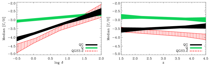
Figure 1: Shaded regions enclose the $1\sigma$ confidence contours for fits to the carbon abundance as a function of overdensity $\delta\equiv\rho/\left<\rho\right>-1$ and redshift for $z=3$ (left) and $\log\delta=0.5$ (right). Results are shown for the fiducial UV background model (QG) for galaxies and quasars, as well as for a pure quasar background (Q) and for a model in which the flux was reduced by a factor 10 above 4 Ryd to mimic incomplete He ii reionization (QGS3.2). Figure taken from Schaye et al. (2003).

Metal lines are clustered on scales up to $\sim 10^{3}~{}{\rm km}\,{\rm s}^{-1}$ (e.g., Pichon et al. 2003; Boksenberg et al. 2003) and their autocorrelation exceeds that expected for a metal distribution that depends only on the density (Scannapieco et al. 2005). Adelberger et al. (2003, 2005) found that the cross-correlation between C iv lines and Lyman-break galaxies increases with $N_{\rm CIV}$ and becomes comparable to the galaxy autocorrelation for $N_{\rm CIV}\gtrsim 10^{12.5}~{}{\rm cm}^{-2}$, which suggests that the strongest C iv lines arise in gas that is directly associated with the galaxies. Motivated by these findings, Pieri, Schaye, & Aguirre (2005) showed that the abundances of C and O depend on both the gas density and the proximity to highly-enriched regions (and thus galaxies). Pieri et al. also found that the parameter “galaxy proximity” can account for part of the scatter in the abundance of carbon at fixed $\tau_{\rm HI}$.

Songaila (2001) found no evidence for evolution in the column density distributions of C iv and Si iv from $z\approx 5$ to 2, although the constraints are poor for $z>4$. The integral of the distribution is insensitive to weak lines and was found to be roughly constant over the same redshift range (Songaila 2001; Pettini et al. 2003; but see Songaila 2005). Although these observations cannot tell us about the evolution of the elemental abundances (see §5.2), they do provide a lower limit to the metallicity of the universe at $z\approx 5$ of $[{\rm C}/{\rm H}]\approx-4$.

Aguirre et al. (2004) compared POD statistics of observed spectra with those of spectra drawn from hydro simulations that use the carbon distribution measured by Schaye et al. (2003), but a variable Si/C ratio. They found that Si is overabundant relative to C and that a single Si/C ratio can reproduce the full distribution of Si iv/C iv. The exact overabundance of Si is sensitive to the hardness of the UV background. It becomes unphysically high for a quasar background, and remains $\gtrsim 0.5$ dex for a background dominated by galaxies. For a soft background, and according to an analysis of O v even for a quasar background (Telfer et al. 2002), O is also inferred to be overabundant relative to C (Bergeron et al. 2002; Simcoe et al. 2004).

Using the POD technique it is possible to detect C iii and Si iii (Songaila 1998). Schaye et al. (2003) and Aguirre et al. (2004) demonstrated that the observed ratios C iii/C iv and Si iii/Si iv rule out temperatures high enough for collisional ionization to dominate, but agree with the predictions for warm, photo-ionized gas. These ratios are also sensitive to the density of photo-ionized gas and the agreement between predictions and observations confirms that the H i absorption arises in the same gas phase as the associated metal absorption. For O vi, on the other hand, the situation is more complicated. At $z\lesssim 2.5$, O vi is detectable in a large fraction of absorbers with $N_{\rm HI}\gtrsim 10^{14}~{}{\rm cm}^{-2}$ and for many of these the observed line widths rule out collisional ionization (Carswell et al. 2002; Bergeron et al. 2002). However, the much rarer O vi systems with $N_{\rm HI}>10^{15}~{}{\rm cm}^{-2}$ often show evidence for a complex, multiphase structure (e.g., Carswell et al. 2002, Simcoe et al. 2002), and the O vi line widths are suggestive of collisional ionization ($T\gtrsim 10^{5}~{}{\rm K}$, Simcoe et al. 2002). Interestingly, a fraction of the O vi associated with low $N_{\rm HI}$ absorbers appear to be metal-rich and too compact to be self-gravitating (Carswell et al. 2002; Bergeron et al. 2002).

5 What are the common misconceptions?

In this section I will discuss a number of common interpretations and claims that, in my opinion, deserve more scepticism than is generally appreciated.

5.1 Gas density

The density at a given point in space depends on the smoothing scale that is used. For example, the density at the point that coincides with the location of this page, will differ enormously depending on whether we smooth over a scale of 1 cm, 1 AU, or 1 Mpc. Therefore, density and volume filling factors are meaningless unless we specify a smoothing scale. Moreover, unless the heavy and light elements are fully mixed, the density of metals and the density of the gas will not have the same dependence on smoothing scale. Unfortunately, smoothing scales are almost never specified, thereby severely limiting the potential usefulness of much of the theoretical and observational literature.

Studies that estimate the density from the column density of fully-resolved H i Ly$\alpha$ lines, effectively smooth their densities on scales corresponding to the sizes of the absorbers, which, for overdense absorbers, should typically be close to the local Jeans length and will therefore depend on the density itself (Schaye 2001):

$$L\sim 1.0\times 10^{2}~{}{\rm kpc}\left({N_{\rm HI}\over 10^{14}~{}{\rm cm}^{-2}}\right)^{-1/3}\left({T\over 10^{4}~{}{\rm K}}\right)^{0.41}\left({\Gamma_{\rm HI}\over 10^{-12}~{}{\rm s}^{-1}}\right)^{-1/3}.$$ (6)

Studies that use the H i Ly$\alpha$ optical depth to estimate the density will effectively smooth the density field twice: once as for column densities and then again on the thermal broadening scale ($\sim 2b/H(z)$). Using equation (1) and the high-redshift approximation $H\propto(1+z)^{3/2}$ for the Hubble parameter, we obtain

$$L_{\rm th}\sim 58~{}h^{-1}\,{\rm kpc}~{}\left({m_{\rm H}\over m}\right)^{1/2}\left({T\over 10^{4}\,{\rm K}}\right)^{1/2}\left({1+z\over 4}\right)^{-3/2}.$$ (7)

Note that in this case the smoothing length depends on the mass of the ion being ionized, which complicates the interpretation. One way to solve this problem is to smooth the spectrum on the thermal scale of the lightest element (e.g., Aguirre et al. 2004). Naturally, if the H i lines are not resolved, then the smoothing scale will be set by the spectral resolution.

5.2 Evolution

Observations suggest that the global densities of C iv (i.e., $\Omega_{\rm CIV}$) and Si iv have not evolved significantly from $z=5$ to $z=2$ (Songaila 2001: Pettini et al. 2003, but see Songaila 2005). These observations are widely quoted to support the idea that the IGM was enriched by small galaxies at very high redshift. However, there are two reasons why the evolution of $\Omega_{\rm CIV}$ (and similarly $\Omega_{\rm SiIV}$) does not tell us much about the evolution of the IGM metallicity. First, the integral over the observed C iv column density distribution diverges at high $N_{\rm CIV}$ if we extrapolate to high column densities. Thus, very large quasar samples are needed to constrain $\Omega_{\rm CIV}$. Moreover, even if such samples were available, they would probe the evolution of the number density of the strongest C iv systems, which are usually associated with Lyman limit systems rather than the diffuse IGM. Second, ionization corrections can be as large as a factor 10 (Schaye et al. 2003). If, as expected for the diffuse IGM, these corrections depend on redshift, then the evolution of $\Omega_{\rm CIV}$ will tell us very little about the evolution of $\Omega_{\rm C}$.

Schaye et al. (2003) did correct for ionization and did not find any evidence for evolution in the distribution of carbon in the diffuse IGM from $z\approx 4$ to 2 for any of their UV background models. However, at $2\sigma$ confidence their results still allow a factor of 2 increase in the abundance of carbon. Considering that the age of the universe roughly doubles from $z=4$ to 2, it is clear that better measurements are needed before we can draw strong conclusions about the epoch of IGM enrichment.

5.3 Percentiles

Suppose that the median C iv optical depth or column density corresponding to some H i bin significantly exceeds the median noise/contamination level, i.e., carbon is detected. What does this imply for the fraction of the absorbers (with the corresponding H i strength) that are enriched? Nearly all studies in the literature have assumed either that all are enriched to this median level, or that 50% of the absorbers are enriched to a level greater than the median. The truth is, however, that we simply do not know. It is possible that the common interpretations are correct, but it is also possible that only a small fraction of the absorbers contain carbon.

Take, for example, a sample of 100 absorbers, all but one of which are metal-free. The median metal abundance will in that case be consistent with zero. Now take a sample of $10^{6}$ absorbers of which 99% are again metal-free. The median can in that case be measured precisely and may significantly exceed the median noise level, but it would clearly be wrong to conclude that at least 50% of the absorbers are enriched. On the other hand, if the observed median C iv strength would exceed the 99.9th percentile of the noise pdf, then the conclusion that at least 50% of the absorbers contain carbon would be justified. These examples show that it is possible to recover information on the filling factor of metals, but that this requires a very careful analysis if the observed metal abundances are close to the detection limit. Up till now, such an analysis has not been carried out and consequently we have no strong constraints on the filling factor of enriched, low-density gas (which dominates the overall filling factor).

5.4 Incompleteness corrections

Observed distributions of column densities are often “corrected” for incompleteness. For example, Monte Carlo simulations have been used to estimate the amount of metal absorption in the form of lines (e.g., Ellison et al. 2000) and pixels (e.g., Songaila 2005) that has been missed due to noise and/or line blending. This procedure is arbitrary because one has to decide down to which column density incompleteness corrections are applied. It is also model-dependent because one has to assume an input distribution for the Monte Carlo simulations. Thus, it is important to check whether observational results have been “corrected” for incompleteness or whether they represent true detections.

5.5 Metal inventory

It is necessary to know the ionization balance in order to convert observed ion abundances into elemental abundances. However, metals residing in gas which is very hot, $T>>10^{5}~{}{\rm K}$, will be so highly ionized that they are essentially invisible in rest-frame ultraviolet absorption spectra. It is therefore important to note that current observational constraints apply only to the warm, $T\sim 10^{4}-10^{5}~{}{\rm K}$, IGM. We cannot rule out the possibility that significant amounts of intergalactic metals are hidden in hot, collisionally ionized gas.

6 Conclusions

The low densities and metallicities that are characteristic of the diffuse IGM make it very difficult to detect heavy elements. Once detected, the interpretation is complicated by the large ionization corrections that are needed to convert observed ion abundances into elemental abundances. Despite these challenges, tremendous progress has been made, driven by the quality of the quasar spectra delivered by echelle spectrographs on 8m-class telescopes, the availability of increasingly realistic hydrodynamical simulations, and the development of sophisticated statistical techniques.

Analyses of absorption by H i, C iii, C iv, O vi, Si iii, and Si iv have revealed that the distribution of metals is highly inhomogeneous, that the metallicity of the IGM is a strong function of the environmental parameters density and proximity to galaxies, that there is not much room for evolution from $z\sim 4$ to 2, and that a substantial reservoir of metals was already in place by $z=5$. We also know that Si, and probably also O, is highly overabundant relative to carbon. While most of the enriched gas clouds are found to be photo-ionized and metal-poor, there is some evidence for hot, collisionally ionized oxygen, particularly at high densities, and there exist some metal-rich clouds which are too compact to be self-gravitating.

Although we have already learned a lot, it is clear that we have only just begun to extract the wealth of information contained even in existing observations. As methods, models, and instruments continue to improve, so will our understanding of the chemical composition of the universe.