The Star Formation Threshold in NGC 6822

Abstract

We investigate the star formation threshold in NGC 6822, a nearby Local Group dwarf galaxy, on sub-kpc scales using high-resolution, wide-field, deep Hi, H$\alpha$ and optical data. In a study of the Hi velocity profiles we identify a cool and warm neutral component in the Interstellar Medium of NGC 6822. We show that the velocity dispersion of the cool component ($\sim 4$ $\,\mbox{km}\,\mbox{s}^{-1}$) when used with a Toomre-$Q$ criterion gives an optimal description of ongoing star formation in NGC 6822, superior to that using the more conventional dispersion value of $6$ $\,\mbox{km}\,\mbox{s}^{-1}$. However, a simple constant surface density criterion for star formation gives an equally superior description. We also investigate the two-dimensional distribution of $Q$ and the star formation threshold and find that these results also hold locally. The range in gas density in NGC 6822 is much larger than the range in critical density, and we argue that the conditions for star formation in NGC 6822 are fully driven by this density criterion. Star formation is local, and in NGC 6822 global rotational or shear parameters are apparently not important.

1. Introduction

In many galaxies, star formation as traced through H$\alpha$ emission is usually only found in the inner parts, whereas the Hi disk is seen to extend to much larger radii. The presence of lower column density gas at large radii, coupled with the absence of obvious star formation there has led to the concept of a star formation threshold: below a certain critical density (which can be constant or varying with radius, depending on the assumptions made) gas is unable to turn into stars. The idea of a star formation threshold has been pursued both observationally and theoretically. For example, Skillman (1987) found that a constant Hi column density value of $\sim 10^{21}$ cm^-2 separated higher column density star forming regions from lower density inert regions. Kennicutt (1989) and more recently Martin & Kennicutt (2001) developed the idea of a star formation threshold originating in the Toomre $Q$ parameter describing gravitational instabilities in a gaseous, rotating disk (see also Quirk 1972). This description is based on comparisons of azimuthally averaged CO/Hi and H$\alpha$ profiles, and thus provides a global picture of the threshold. Note that in some galaxies isolated Hii regions are found in regions with gas densities below the (azimuthally averaged) threshold value (e.g. Ferguson et al. 1998): these may occur at positions where the local conditions are favourable to star formation. The recent discovery of recent star formation in the outer disks of M83 (Thilker et al., 2005) and NGC 4625 (Gil de Paz et al., 2005) additionally suggests that H$\alpha$ may not be a complete tracer of ongoing star fomation in disk galaxies. Other evidence for extended star formation in irregular dwarf galaxies by tracing blue “clumps” is presented in Parodi & Binggeli (2003).

In this paper we investigate the star formation threshold in NGC 6822. In a companion paper [de Blok & Walter 2005 (Paper I)] we have presented high-resolution Hi, H$\alpha$ and optical datasets that give for the first time a detailed picture of the distribution of gas, recent star formation and the resolved stellar population in this galaxy.

We refer to Paper I for a description and presentation of these data. In summary, the Hi data set consists of an 8-pointing mosaic obtained with the Australia Telescope Compact Array. The data have a spatial resolution of $42^{\prime\prime}\times 12^{\prime\prime}$ and a velocity resolution of 1.6 $\,\mbox{km}\,\mbox{s}^{-1}$and show the presence of an extended Hi disk. The optical data consists of $B$, $R_{C}$, and $I$ observations obtained with Suprime-Cam on the Subaru telescope. These resolve the stellar population in NGC 6822. By isolating stars with $(B-R)<0.75$ and $18\lesssim m_{B}\lesssim 26$ (no extinction corrections applied), we show the presence of a young, blue population spread throughout the entire extended Hi disk in a highly structured fashion. This population consists of main sequence stars with luminosities $-7\lesssim B\lesssim+1$, corresponding to O to A stars with main-sequence life-times from $\sim 1$ to $\sim 100$ Myr. Our wide-field H$\alpha$ data (obtained with the Widefield Camera on the Isaac Newton Telescope) show the presence of several hitherto unknown Hii regions in the outer HI disk.

Here we bring these data sets together in a study of the star formation threshold. In many ways NGC 6822 is an ideal galaxy for testing the various explanations and incarnations of the star formation threshold. It is a nearby Local Group dwarf galaxy unaffected by the presence of a bulge or spiral arms that could complicate the interpretation of its dynamics. Its small distance of only 490 kpc enables us to study the Interstellar Medium (ISM) and the stellar population on scales of $\sim 100$ pc or less, i.e., the scale of Giant Molecular Clouds.

In the next section we discuss various observational and theoretical interpretations of the threshold. Section 3 deals with the decomposition of the Hi velocity profiles and the identification of a cool and warm component of the neutral ISM in NGC 6822. Section 4 discusses the radial as well as the two-dimensional distribution of the star formation threshold. We summarise our results in Sect. 5.

2. Interpretations of the star formation threshold

The most popular explanation of the star formation threshold is based on the Toomre $Q$ parameter. This parameter is defined as

$$Q(r)={{c_{s}\kappa}\over{\pi G\Sigma_{g}}},$$ (1)

where $c_{s}$ is the sound speed in the gas, $G$ the gravitational constant, $\Sigma_{g}$ the surface density of the gas and $\kappa$ is the epicyclic frequency, defined as $\kappa^{2}=2(V/R)^{2}[1+(R/V)(dV/dR)]$. Itself, $\kappa$ is a function of the rotation curve $V(R)$. In this picture, a disk will be unstable against radial perturbations if $Q<1$, and one can define a critical density for star formation

$$\Sigma_{c}=\alpha{{c_{s}\kappa}\over{\pi G}}.$$ (2)

The constant $\alpha$ is used to reconcile the model with the observations. In most analyses, including this one, the one-dimensional velocity dispersion $\sigma$ is used instead of $c_{s}$. Schaye (2004) makes the explicit correction $c_{s}=\sigma\sqrt{\gamma}$, where $\gamma=5/3$ is the ratio of specific heats for an adiabatic mono-atomic gas. We prefer to use $\sigma$, keeping in mind that the sound speed correction is taken up into the value of $\alpha$.

In essence, Eqs. (1) and (2) describe the ability of perturbations to rotate around their centre, and thus their stability against collapse. Kennicutt (1989) applied this prescription to a number of spiral galaxies and compared the radial distributions of the ratio of the critical density $\Sigma_{c}$ and the neutral gas density $\Sigma_{g}$ with the distribution of H$\alpha$ in 15 spiral galaxies. He found that for a value of $\alpha=0.63$ he could correctly describe the steep drop-off in star formation at the H$\alpha$ truncation radius for most galaxies. This work was later extended and confirmed by Martin & Kennicutt (2001) who studied a sample of 32 nearby spiral galaxies. Exceptions do exist though: Martin & Kennicutt (2001) point out that a few nearby spirals with active and organised star formation (e.g. NGC 2403 and M33) have sub-critical densities throughout their disks.

In the context of a critical threshold, star formation is often thought to be self-regulatory and striving for a $Q\sim 1$ situation. Regions where $Q<1$ will form stars, diminishing the local gas density, and increasing the local velocity dispersion due to mechanical stirring and true heating. All this will eventually quench star formation. A new build-up of gas, e.g. due to nearby star formation, can then restart the whole process again.

The critical threshold is also used to explain the low star formation rate found in LSB galaxies. van der Hulst et al. (1993) found that in these galaxies the gas surface densities were below the critical density over most of their disks. Local density enhancements were thought to provide the necessary instability for stochastic star formation.

An alternative description of the threshold is given by Hunter, Elmegreen & Baker (1998). They analysed a sample of dwarf and irregular galaxies and needed a value of $\alpha$ which was a factor $\sim 2$ lower than the Kennicutt (1989) value to explain their results in the context of a $Q$ parameter (though part of this difference is due to the different velocity dispersion value they used). They argue that for their galaxies the local shear rate gives a much better description of the ability of perturbations to collapse. This shear threshold is defined in a similar way as the threshold in Eq. (2), with $\kappa$ replaced by $\pi A$, where $A=-0.5\,R\,(d\Omega/dR)$, one of the Oort constants, where $\Omega$ is the angular speed.

Much effort has also been put into finding a physical basis for the star formation threshold. The most promising one seems to involve the phase structure of the ISM, as pointed out by Elmegreen & Parravano (1994), and emphasized by Gerritsen & Icke (1997); Hunter et al. (1998, 2001); Billett et al. (2002) and Elmegreen (2002). Recently, several of the observational and theoretical strands were drawn together in a paper by Schaye (2004). Its major points that are relevant for the current analysis can be summarised as follows.

The main conclusion from Schaye (2004) is that star formation can only happen if the ISM contains a cool phase (see also Taylor & Webster 2005). The transition to a cool phase is associated with a steep drop in the thermal velocity dispersion, which causes instabilities on a wide range of scales, and is the physical cause for the drop in $Q$ at the critical radius in the models. This implies that in determining $Q$ the relevant parameter is the thermal velocity dispersion of the cool phase of ISM. The dispersion that is usually used, as derived from straight-forward second-moment maps, is predominantly caused by the warm neutral ISM, and will therefore usually be higher than that of the cool component. The simple second-moment velocity dispersion values are therefore not necessarily applicable to a star formation threshold analysis.

In local hydrostatic equilibrium with only a warm phase present, there is a direct relationship between density, surface density and pressure. For fixed temperature, gas fraction, metallicity and UV field the formation of a cool phase depends only on density, and therefore surface density. Flaring of the disk is, in these models, only expected to occur beyond the critical radius, where the temperature increases steeply; for the purposes of this discussion the scale height of the disk is thus constant within the critical radius. In the models, the drop in velocity dispersion thus occurs at a fixed critical surface density. This surface density agrees with the values derived observationally. Rotation (i.e. Coriolis force and shear) cannot prevent a cool phase from forming within the critical radius: the rotation curve and epicyclic frequency change smoothly across this radius. As the threshold therefore only depends on surface density, it must be a local phenomenon. Any peak that exceeds the critical surface density has the potential to form stars, regardless of its position. As Schaye (2004) notes, the model predicts its own demise: once stars form, feedback in a complex multi-phase ISM is not well described by a simple model. One should thus not necessarily expect the critical density recipe to work in regions of active starformation. In the models, the critical hydrogen surface density for star formation is $\log(N_{H})\simeq 20.75$ ($\sim$ 4.5 $M_{\odot}$ pc^-2), but depends slightly on metallicity, ambient radiation field, and gas fraction.

Lastly, the reason why the conventional interpretation of the threshold with its (too high) constant velocity dispersion does yield correct values for the critical radii, is shown in Fig. 3 of Schaye (2004). The change in $Q$ with radius is shown there, both for the choice of velocity dispersion motivated by the model, as well as the conventional assumption of a constant velocity dispersion. The latter choice gives a $Q$ that increases gradually with radius, and at the critical radius intersects the steeply dropping model $Q$ value. As the drop in this “true” $Q$ is so steep and sudden, the conventional $Q$ curve will always intersect it at the critical radius, independent of the choice of observed velocity dispersion. It will furthermore do this at $Q=1/\alpha$. Choosing the appropriate value for the velocity dispersion (namely that of the cool phase), and making the correction for the sound speed (see Sec. 2) makes the intersection happen at $Q=1$. For example, the Kennicutt (1989) value of $\alpha=0.63$ was derived assuming a dispersion of 6 $\,\mbox{km}\,\mbox{s}^{-1}$. Correcting this for the sound speed, yields $\alpha\simeq 0.5$. Using a lower velocity dispersion of $3-4$ $\,\mbox{km}\,\mbox{s}^{-1}$, as appropriate for the cool phase, leads to $\alpha\simeq 1$.

In summary, an increase in density in the warm phase leads to an onset of a cool phase, accompanied by a steep drop in velocity dispersion, resulting in a lower value of $Q$. This occurs at a fixed surface density, and does not depend on rotation. The star formation threshold is a local phenomenon.

3. HI profiles and velocity dispersion

The integrated Hi map and the velocity field of NGC 6822 are presented in Paper I (see also Weldrake et al. 2003). They show an extended Hi disk characterized by the presence of the NW companion — a dwarf galaxy interacting with the main body of NGC 6822 — and a super-giant shell, presumably caused by the effects of star formation, dominating the SE part of the disk. The velocity field shows that the galaxy is in regular solid-body rotation.

From the Hi data presented in Paper I we can also derive a second-moment map (where the second moment is defined as $\sqrt{\langle V^{2}\rangle-\langle V\rangle^{2}}$). This map is shown in Fig. 1. It should be compared with the integrated HI map and velocity field as well as the maps of the stellar distribution presented in Paper I. The highest second-moment values ($>8$ $\,\mbox{km}\,\mbox{s}^{-1}$) are found in the region roughly corresponding with the optically prominent part of the disk, whereas the NW companion, the large hole and the SE tidal tail are characterised by values $<8$ $\,\mbox{km}\,\mbox{s}^{-1}$. The median second-moment value in the Hi disk is 6.7 $\,\mbox{km}\,\mbox{s}^{-1}$. For simple, single-component Gaussians, these second-moment values can be directly interpreted as physical dispersion values. However, for more complicated profiles, second-moment values, even though often still called “dispersions”, should be treated with care. For non-Gaussian or multi-component profiles (which are ubiquitous in NGC 6822 as we will show below) the interpretation of second-moment values as dispersions is not always unambiguous. Furthermore, in a multi-phase medium with star formation the measured velocity dispersion is the sum of the dispersions of the cool and warm phase with additional input from star formation and turbulence. As the relevant dispersion value to use in a star formation threshold analysis is that of the cool phase of the ISM, using the second-moment values will likely result in significant over-estimates. A simple second-moment analysis is not sufficient for the current investigation, and a more precise analysis of the HI velocity profiles is needed.

3.1. High-velocity gas

In order to study the threshold for star formation by means of the Hi velocity profiles it is essential to concentrate only on those parts of the galaxy where the analysis is valid. Regions where the ISM is heavily disturbed are less suited, as the velocity dispersion is less likely to reflect the intrinsic state of the ISM, but rather bulk motions of gas along the line of sight. Disturbed gas can usually be identified by velocities that significantly deviate from the local rotation velocity.

To locate this high-velocity (HV) gas in NGC 6822 we have used the data cube presented in Paper I, and isolated all emision brighter than 3 times the RMS noise level and more than 18 km s^-1 (or 3$\sigma$, assuming $\sigma=6$ km s^-1) away from the local rotation velocity.

The top-left panel in Fig. 2 shows the location of this HV gas overlaid on the normal Hi surface density map of NGC 6822. We distinguish between HV gas with positive and negative deviation from the rotation velocity, but Fig. 2 shows that the majority of the HV gas has a positive deviation.

The top-centre and top-right panels in Fig. 2 compare the position of the HV gas with the distributions of the H$\alpha$ emission and the young, blue population (as described in Sect. 1 and Paper I), respectively. It is obvious that most of the HV gas is associated with H$\alpha$, though not necessarily with the strongest emission. This contrasts with the distribution of the young, blue stars, which seems to be anti-correlated with the HV emission. The H$\alpha$ emission has a clear minimum at the positions of the two most prominent concentrations of blue stars at the tips of the central bar-like structure. These correlations could indicate a rapid infall of any HVC gas back into the disk, or may be an indication for ionization of the gas.

The most prominent HV feature is a partially ring-like structure found in the southern part of the disk. Its signature is consistent with that of chimney due to star formation. The proximity to the so-called Blue Plume (indicated in the top-right panel in Fig. 2), one of the most active regions of star formation in NGC 6822, make it likely that the combined effects of star formation in this area have caused this feature. The similarity in size between the Plume and the chimney supports this idea. If this association is correct, then the chimney is not caused by a single star cluster, but by a large conglomerate of young stars $\sim 0.5$ kpc in diameter.

The bottom panel shows a number of cross-cuts in the form of position-velocity diagrams. As we step along the slices from north to south we first see the appearance of a single component of HV gas, which then splits up in what appear to be two walls of a chimney (slice 5), which then merge again into a single component. Beyond this, there is an extended tail of HV gas which in projection extends beyond the Hi disk, but which in reality is likely to have been removed vertically from the chimney.

If the latter is the case, and given that the deviation with respect to the rotation velocity is positive, the assumption that the gas is still positioned more or less over the chimney, then leads to the conclusion that the HV gas is situated on the far side of the disk. This would mean that the southern part of the disk of NGC 6822 is the part closest to us. We can use the average inclination and PA values as given in Weldrake et al. (2003) ($i\simeq 60^{\circ}$ and PA $\simeq 135^{\circ}$) to show that the HV gas plume must then be $\sim 170$ pc above the disk. Comparing with the value for the Hi scale height of 0.28 kpc derived in de Blok & Walter (2000), shows that this gas is still close to the disk, and will most likely fall back.

3.2. Profile Decompositions

To extract the Hi velocity profiles we Hanning-smoothed the cube to reduce the impact of Galactic residuals, and regridded to a pixel size of $48^{\prime\prime}$, thus ensuring that every spatial pixel contains an independent profile. To isolate the positions containing sufficient signal for this analysis, we restrict ourselves to profiles whose peak flux is four or more times the RMS noise per channel.

Profiles were fitted with both a one-component and a two-component Gaussian model. The majority of the profiles turned out to be non-Gaussian. A comparison between the goodness-of-fit parameters of both sets of fits showed that of the 732 profiles, 241 could be fitted equally well with either one or two components (that is to say, their reduced $\chi^{2}$-values agreed to within 10 percent). For 438 profiles the two-component fit produced significantly lower reduced $\chi^{2}$ values than the single component fit (i.e. a difference larger than 10 percent). For 53 profiles a one-component fit was preferred. The formal error in the dispersion for the two-component fits is $\sim 0.6$ $\,\mbox{km}\,\mbox{s}^{-1}$, much less than the dispersions measured.

Figure 3 compares the quality of the one- and two-component fits. The dots indicate the positions of the profiles. The profiles where the two-component fit is preferred are spread across most of the galaxy. Profiles where a one-component fit performs better are only found in the SE tidal arm. This is also the region where residual Galactic foreground emission affects the velocity profiles significantly (cf. Fig. 2 in Paper I), and this, rather than any physical explanation, is the cause of the better performance of the one-component fits. In the following we will therefore stay clear of a physical interpretation of the profiles in the tidal arm.

The profiles where one- and two-component fits perform equally well tend to be found towards the outer parts of the disk, notably the northern edge of the NW companion and the eastern rim of the supergiant shell. However, there is no clear correlation between the presence of e.g. star forming regions and number of components. The only obvious conclusion one might draw is that the two-component fits tend to be preferred in regions with a higher blue stellar surface density (compare Fig. 3 with the top-right panel of Fig. 2).

Figure 4 shows a representative subset of profile shapes. Most of them are non-Gaussian and seem to consist of a narrow component superimposed on a broader one (e.g. the profiles in the bottom-right of Fig. 4), while others are asymmetric (top-left) or even double-peaked (bottom-left).

Figure 5 shows an example of a profile where a two-component model is clearly preferred. Inspection of the individual fit-components shows that one is characterized by a large velocity dispersion $\sigma\sim 12$ km s^-1, while the other has a narrow dispersion $\sigma\sim 5$ km s^-1. This is a general feature of the profiles: for the majority a decomposition using a two-component Gaussian model results in a broad and a narrow component.

Figure 6 shows histograms of the velocity dispersions of both components, superimposed on the distribution derived from a one-component Gaussian fit. The latter is very close to the distribution of dispersions one would derive from the second-moment map (Fig. 1). The narrow component in Fig. 6 has a mean velocity dispersion value of 4.4 km s^-1 with an RMS of 1.8 km s^-1. The broad component has a mean of 8.2 km s^-1 with an RMS of 2.4 km s^-1. There is some overlap between the two components, this is mostly due to profiles that are double peaked (such as the ones in the centre-left of Fig. 4). Here the fit does not capture narrow and broad components but rather traces the bulk motion of gas clouds along the line of sight due to e.g. effects of star formation.

The small size of the beam with respect to that of the galaxy (48^′′ equals 110 pc at the NGC 6822 distance) and the shallow rotation curve rule out that we are looking at lines that are rotationally broadened. With an inclination of $\sim 60^{\circ}$ the maximum projected beam size in the plane of NGC 6822 is 220 pc, small enough to rule out that we are looking at kinematically uncorrelated components within the beam. Due to the peak flux cut-off used in making the fits, the total Hi mass recovered by the fits is smaller than the total Hi mass of NGC 6822. The two component fits retrieve 71 per cent of the total mass, or $9.5\cdot 10^{7}$ $M_{\odot}$. Of the recovered mass, 29 per cent (or $2.8\cdot 10^{7}$ $M_{\odot}$) forms the narrow dispersion component, while 71 per cent ($6.7\cdot 10^{7}$ $M_{\odot}$) is found in the broad dispersion component.

Most of the overlap between the histograms in Fig. 6 is due to double-peaked profiles. Based on Fig. 6 we thus introduce an alternative division between the narrow and broad component by defining as “narrow” all those profiles with $\sigma\leq 6$ km s^-1 and as “broad” those with $\sigma>6$ km s^-1. Using this alternative definition 19 per cent of the retrieved Hi (or $1.8\cdot 10^{7}$ $M_{\odot}$) forms the narrow dispersion component, while 81 per cent ($7.7\cdot 10^{7}$ $M_{\odot}$) is found in the broad dispersion component. These ratios are very similar to the ratios found in previous studies of broad and narrow components in dwarf galaxies (e.g., Young & Lo 1996, 1997).

3.3. Broad and narrow components

Figure 7 shows the distribution of the narrow and broad components, using the 6 km s^-1 definition. The lack of emission in the SE corner (corresponding to the location of the tidal tail) is due to the presence of residual Galactic foreground emission making the interpretation of the fits there problematic (cf. Fig. 3). In the following we will concentrate on the emission in the other, unaffected parts of the area. The broad component seems more widely, and more continuously distributed. A slight anti-correlation between the components seems present: most (though not all) of the high-column density narrow dispersion emission is found at positions of lower broad-dispersion intensity, and vice versa.

Figure 7 should be interpreted with care though, and compared with Fig. 2. In most of the disk the decomposition in two components reflects the local state of the neutral gas component, but as Fig. 2 shows, in regions in the central parts of the disk where double-peaked profiles are found, the interpretation is less straight-forward. For example, the prominent peak in the low-dispersion component around $(\alpha,\delta)=$ $19^{h}44^{m}50,-14^{\circ}55^{\prime}40^{\prime\prime}$ occurs in a region where a significant high-velocity gas component is present (see Sect. 3.1).

In all of this it should be kept in mind that the resolution of the data and the rebinning to 48^′′ may lead to an underestimate of the importance of the narrow dispersion component, as does the complex velocity structure in the inner parts.

The narrow dispersion component has a patchy distribution but is generally found throughout the star forming disk. Fig. 7 also compares the distribution of the narrow dispersion component with that of the H$\alpha$ emission and the blue stars. Except for the aforementioned prominent peak where interpretation is made difficult by the presence of high-velocity gas, every other low-dispersion peak has a compact H$\alpha$ region in its direct environment (though the reverse is not always true). This even holds for the low surface brightness H$\alpha$ regions in the NW companion and on the SE rim of the giant hole. The narrow dispersion component also seems to avoid regions of high densities of young stars.

In the following we will associate the narrow dispersion component we have identified in NGC 6822 with the cool phase of the neutral ISM. We will adopt an average value of 4 $\,\mbox{km}\,\mbox{s}^{-1}$ as the velocity dispersion of the cool component in our analysis of the star formation threshold (see Fig. 6).

4. The Critical Density

4.1. Radial Distributions of Critical Density

Figure 8 compares the radial distribution of the neutral gas with that of the critical density as defined in Kennicutt (1989) and the shear critical density investigated in Hunter et al. (1998). For both we have used the $12^{\prime\prime}$ rotation curve and Hi surface density profile presented in Weldrake et al. (2003). The gas density was derived from the inclination-corrected Hi surface density profile by multiplying the latter with 1.4 to correct for the presence of helium and metals. We show the critical densities for a dispersion value $\sigma=6$ $\,\mbox{km}\,\mbox{s}^{-1}$, used in much previous work and consistent with values derived from a simple second-moment analysis, and a value of 4 $\,\mbox{km}\,\mbox{s}^{-1}$, as derived above for the cool neutral ISM component in NGC 6822.

Additionally we show the Schaye (2004) critical density $\log(N_{H})=20.75$, also corrected for He and metals. We compare these with the radial distributions of H$\alpha$ and the number density of blue stars. The radial profiles were derived using the same tilted ring parameters that were used to derive the rotation curve.

There a few things to note: the distribution of H$\alpha$ is fairly constant in the inner part of NGC 6822, then drops suddenly at $R\simeq 2.0$ kpc, and runs out at $R\simeq 2.7$ kpc. The NW companion is visible as a very slight rise around $\sim 4.4$ kpc. The distribution of the number density of blue stars changes more gradually and only reaches zero level at the edge of the Hi disk. Note that the shape of the blue stars profile is very similar to that of the Hi profile. This will be discussed briefly below. Qualitatively the difference between the shape of the H$\alpha$ profile and that of the blue stellar surface density profile bears a striking resemblance with the discrepancy between the H$\alpha$ and GALEX UV profiles in M83 (Thilker et al., 2005), suggesting that the surface density of blue stars is a good proxy for the UV surface brightness in NGC 6822. Future UV observations will have to confirm this.

Both the Toomre-$Q$ and the shear interpretations of the critical density yield very similar profiles. The exact value of the critical density in the shear interpretation is slightly uncertain though, due to different definitions used by different authors. The definition used in Hunter et al. (1998) results in values that are $\sim 20$ per cent lower than those derived using the Schaye (2004) definition. Here we plot only the latter.

The interpretation of these profiles depends on the value of the velocity dispersion used. If we assume $\sigma=6$ $\,\mbox{km}\,\mbox{s}^{-1}$, then we would conclude that the disk is stable against star formation everywhere. This would make NGC 6822 comparable with the LSB galaxies studied by van der Hulst et al. (1993). A physical interpretation of this result would be that just as in the LSB galaxies, local density enhancements should provide the trigger for star formation. These enhancements would be averaged out in a radial profile, giving the impression of an entirely stable disk.

Assuming $\sigma=4$ $\,\mbox{km}\,\mbox{s}^{-1}$, leads to a lower critical density. For radii $R<2$ kpc both the Kennicutt (1989) and Hunter et al. (1998) critical densities follow the gas density rather closely. In this case a possible physical interpretation would be that star formation is self-regulating, and strives for a $Q\sim 1$ situation. At $R\gtrsim 2.5$ kpc the gas profile rapidly falls away from the critical density profiles. Clearly, the outer disk is strongly sub-critical for both values of $\sigma$, at least in the azimuthally averaged formulation of the star formation threshold.

Note that for the 4 $\,\mbox{km}\,\mbox{s}^{-1}$ case, the gas profile starts to drop away from the Toomre-$Q$ critical density at the same radii as where the H$\alpha$ runs out (between 2.0 and 2.2 kpc). This is very close to the radius where the gas surface density curve crosses the Schaye (2004) critical surface density value. For $\sigma=4$ $\,\mbox{km}\,\mbox{s}^{-1}$, both the Kennicutt (1989) and Schaye (2004) indicators of the threshold thus give identical results, at least where the critical radius is concerned. Note that over the radial range examined here the variation in gas surface density (a factor $\sim 20$) is much larger than the variation in critical density (a factor $\sim 2.5$). This implies that variations in gas surface density are potentially more important in determining $\Sigma_{g}/\Sigma_{c}$ than variations in the critical density itself. In the following we will restrict ourselves to the Kennicutt (1989) threshold.

Lastly, a word of caution: as was stressed by Schaye (2004), his model implies its own failure: when stars form, complex feedback effects and the presence of a many-phase ISM, invalidate many of the basic assumptions behind it. The star formation threshold in all its incarnations should only be regarded as a tool that indicates where there is potential for star formation on intermediate and large scales ($\gtrsim 0.5$ kpc or so). Precise predictions on where the next star forming region will form are beyond its scope.

4.2. Blue stars and HI surface density

In the previous sub-section we commented on the remarkable similarity between the shapes of the radial Hi profile and the radial blue stellar surface density profile. Here we emphasise that similarity in a brief digression from our main star formation threshold topic.

Figure 9 shows the inclination-corrected and helium-corrected gas surface density profile, as well as the inclination-corrected radial profile of the blue stellar surface density. It is clear that the stellar surface density decreases much more rapidly than the gas surface density profile, perhaps indicating a decreased star formation efficiency at lower gas densities.

A simple linear scaling shows however that the shapes of these curves are actually virtually identical. Applying a scaling of the form $\log(\sigma_{\rm stars}^{\rm scaled})=0.49\log(\sigma_{\rm stars})+0.77$ to the stellar surface density curve yields a very good match to the gas surface density profile, with a RMS scatter of only 0.067 in $\log\sigma$, equivalent to 15 per cent. This scaling is equivent to a Schmidt-type law of the form $\sigma_{\rm stars}=0.027\cdot\sigma_{\rm gas}^{2.04}$. It is remarkable that the scatter in this relation is so low and holds over 3 orders of magnitude in stellar surface density, given the many intermediate steps needed to go from an Hi disk to a young star (i.e. molecular cloud formation, collapse, etc). Alternatively, this well-defined similarity between stellar surface density and Hi surface density might indicate that Hi and star formation are more intimately related than usually assumed (see e.g. Allen 2001).

A similar but less well-defined relation holds between the surface brightness of the young stellar population and the Hi surface density (Fig. 9). The scaling does however only work for $R<3.2$ kpc; the blue stars in the NW companion have a surface brightness that is over a magnitude brighter than one would derive on the basis of the scaling. Applying the scaling $\log(\sigma_{\rm stars}^{\rm scaled})=-0.19\cdot\mu_{\rm stars}+5.1$, we find that for radii $R<3.2$ kpc the RMS scatter is 0.089 in $\log\sigma$ ($\sim 22$ per cent). The relation between the total surface brightness and the Hi surface density shows the expected declines in densities towards the outer parts, but does not show the tight coupling described above.

It is remarkable that in NGC 6822 we can so clearly distinguish these various aspects of star formation: the inner parts show a well-defined Schmidt-type law, where the surface density of young stars is directly related to the Hi surface density, with the outer parts showing a pronounced star formation threshold. The latter is particularly well-defined when one considers the local densities of gas and stars. This is what we will return to now.

4.3. Two-dimensional thresholds

With some assumptions we can investigate the local conditions for star formation, i.e., we can extend the one-dimensional star formation threshold to a two-dimensional equivalent. As Eq. (1) shows, the relevant parameters are $\kappa$ and $c_{s}$ (or $\sigma$, remarks below Eq. 2 in Sect. 2). For the dispersion we can either assume a constant value of 4 or 6 $\,\mbox{km}\,\mbox{s}^{-1}$, or use the second-moment map shown in Fig. 1 (though as discussed in the previous sections, the last two choices may not be as appropriate; here we show them only as a comparison with the 4 $\,\mbox{km}\,\mbox{s}^{-1}$ results).

To determine $\kappa$ we would ideally use the velocity field to measure $V$ as a function of radius and position angle, i.e. $V=V(R,\phi)$, and so determine a local $\kappa$ to calculate a local critical density. Unfortunately, due to the well-known projection effects, we can in practice only do this with sufficient accuracy in a relatively small angular range around the major axis. The rotational signal at other position angles becomes too small, and even vanishes near the minor axis.

To determine a local threshold we thus have to make the assumption that $\kappa(R,\phi)=\kappa(R)$, and use the azimuthally averaged tilted ring rotation curve. This potentially limiting assumption is however more than compensated for by the fact that we can use the two-dimensional Hi distribution to compute $\Sigma_{g}/\Sigma_{c}$. Furthermore, the fact that an azimuthally averaged rotation curve could be constructed with fairly small errorbars (see Weldrake et al. 2003) already indicates that azimuthal variations are not large, and certainly not large enough to dominate over azimuthal variations in Hi surface density.

We have computed maps of the local ratios of $\Sigma_{g}/\Sigma_{c}$. Figure 10 shows $\Sigma_{g}/\Sigma_{c}=1$ contours overlaid on the Hi surface density map for the cases of constant velocity dispersions $\sigma=4$ and 6 km s^-1, as well as a variable dispersion derived from the second-moment map in Fig. 1.

The conclusions are similar to the azimuthally averaged case discussed above. For the $\sigma=6$ $\,\mbox{km}\,\mbox{s}^{-1}$ case, only a small fraction of the disk (mostly towards the edge of the Hi disk) is unstable to star formation. The variable dispersion case does not improve matters, the higher dispersions in the inner part of the galaxy make the gas there apparently more stable against collapse.

In the constant dispersion cases, and most prominently for the 4 $\,\mbox{km}\,\mbox{s}^{-1}$ case, a much larger fraction of the disk now has the potential to participate in star formation. As the surface density criterion is a local criterion it can also be applied to the NW companion, even though it is an independent system. We see that the NW companion is indeed unstable to star formation, as confirmed by the presence of H$\alpha$ and young stars there.

In the following we will restrict ourselves to the constant dispersion thresholds. In Fig. 11 we compare the distribution of $\Sigma_{g}/\Sigma_{c}$ with those of H$\alpha$ and the blue stars as well. The left panels show $\Sigma_{g}/\Sigma_{c}=1$ contours for a 6 $\,\mbox{km}\,\mbox{s}^{-1}$ dispersion. The right-hand panels show the same for a 4 $\,\mbox{km}\,\mbox{s}^{-1}$ dispersion. Overall, the 4 $\,\mbox{km}\,\mbox{s}^{-1}$ contours give a much better description of the locations of (recent) star formation activity than the 6 $\,\mbox{km}\,\mbox{s}^{-1}$ contours. Note the anticorrelation between blue star density and unstable regions for the 6 $\,\mbox{km}\,\mbox{s}^{-1}$ case. Overall, the threshold seems to work best in the outermost parts. Formally speaking the epicycle frequency diverges at small $R$ and the assumption that the disk is thin breaks down. de Blok & Walter (2000) derive a scale height of 0.28 kpc for NGC 6822, meaning that for $R\lesssim 0.5$ kpc the threshold analysis is not valid.

The right-hand panels of Fig. 11 also show the surface density threshold described in Schaye (2004). Plotted is the $\log(N_{HI})=20.75$ surface density contour (corrected for inclination and assuming that Hi is the main component of the H distribution). The unstable area comfortably encompasses the H$\alpha$ and blue stars. Note the very good correspondence with the 4 $\,\mbox{km}\,\mbox{s}^{-1}$ dispersion contours (although the surface density criterion seems to perform slightly better in the inner parts compared with the distribution of blue stars). Just as in the azimuthally averaged picture, we again see that the critical radii in both cases become equivalent when the proper choice for velocity dispersion is made. Also note that the critical radius as defined here corresponds very closely with the edge of the Hi disk.

We can investigate whether these conclusions also hold locally by looking at the pixel-to-pixel correlations between the various components. We have regridded the HI, H$\alpha$ as well as the critical density and blue star density images to a common pixel size of 12^′′.

The left panel in Fig. 12 shows the local correlation between Hi and H$\alpha$ on scales of $12^{\prime\prime}$ ($\sim$ 30 pc). The 1$\sigma$ noise in the background sky level is indicated in the figure. Again we see clear evidence of a well-defined star formation threshold. At $\log(N_{HI})\approx 20.9$ (20.7 after inclination correction) the maximum H$\alpha$ flux per pixel suddenly increases sharply (roughly 1 dex over only 0.15 dex increase in Hi column density). At lower densities only very marginal amounts of H$\alpha$ are present. The arrow in the left panel indicates the predicted value of the Schaye (2004) threshold with the associated errorbars indicated. There is again good agreement between observed and predicted values.

The centre panel shows the pixel-to-pixel relation between $\Sigma_{g}/\Sigma_{c}$ and H$\alpha$, assuming $\sigma=4$ $\,\mbox{km}\,\mbox{s}^{-1}$. Again, the two threshold alternatives yield very similar results. In the right panel in Fig. 12 we show the relation between $\Sigma_{HI}$ and $\Sigma_{c}$. Both axes span the same range, but we see that the variation in critical density is much smaller (by a factor $\sim 200$) than that in Hi density. This behaviour was already discussed for the azimuthally averaged case, but is now also seen to hold locally.

These results again show that changes in $\Sigma_{g}/\Sigma_{c}$ are completely dominated by changes in $\Sigma_{g}$ and that, at least in the case of NGC 6822, the gas density seems to be the ultimate driver for star formation, independent of rotation. Interpreting this in the framework of the Schaye (2004) models, the relevant value of $Q$ is completely determined by $\sigma$, and its steep drop at the onset of the cool phase. The variation in the other parameters that form $Q$ are not important.

5. Summary

We have presented a comprehensive analysis of the star formation threshold in the Local Group dwarf galaxy NGC 6822. The absence of complicating spiral density waves, bar motions, strong shear, etc., make NGC 6822 an ideal target for such a study. The proximity of the galaxy furthermore allows us to investigate the threshold at very high spatial resolution ($<100$ pc).

Regions with High Velocity gas (i.e., with velocities deviating more than 18 km s^-1 from the rotation velocity) were found to be in the vicinity of current star formation (as traced through H$\alpha$) although no one-to-one correspondence exists. This is exemplified by the presence of an Hi ‘chimney’ for which no single parental cluster/association can be easily identified, although it is likely that the combined effects of a larger-scale region of recent star-formation may have created this feature.

The cool and warm phases of the Hi are identified by fitting two-component Gaussians to the Hi profiles. In doing so we find two components, one broad component with a mean dispersion of 8 km s^-1 and a narrow component at 4 km s^-1. A comparison with the H$\alpha$ maps shows that every region with a dominant low-dispersion Hi peak has a compact Hii region in its immediate environment.

We have compared various descriptions of the star formation threshold (Toomre-$Q$, shear, constant density threshold) to radial averages of the Hi and ongoing star formation (as traced by H$\alpha$) and find that of the thresholds that are based on the dynamics of the galaxy, the Toomre criterion with a low velocity dispersion of 4 km s^-1 (our ‘cool’ component) fits the distribution of star formation in NGC 6822 best. However, the predictions of that model are virtually identical to those of the model assuming a simple constant star formation surface density threshold of $\log N_{HI}=20.75$.

Part of the agreement is due to the fact that the critical density $\Sigma_{\rm crit}$ as derived through, e.g., the Toomre criterion, has a much smaller dynamic range than the measured gas surface densities $\Sigma_{\rm gas}$. Changes in the ratio $\Sigma_{\rm crit}/\Sigma_{\rm gas}$ are thus completely dominated by the change in $\Sigma_{\rm gas}$. For the radial profiles, we also find a striking correspondence between the Hi density and the number density of blue stars, showing that these two components are intimately linked to each other in NGC 6822.

Our data also allow us, for the first time, to calculate high-resolution two-dimensional maps of the critical density in NGC 6822. Our finding is similar to those for the radial profiles, in the sense that a Toomre criterion (using a dispersion of 4 km s^-1) gives very similar results compared to a simple star formation threshold of $\log(N_{HI})=20.75$, also locally. This emphasizes that the star formation threshold in NGC 6822 does not depend on rotation but is a purely local phenomenon. One needs to keep in mind though that the current analysis was done for one dwarf galaxy only. Even though the observations are exquisite in the details they show, results drawn from this study will need to be confirmed by similar analyses on other dwarf galaxies.

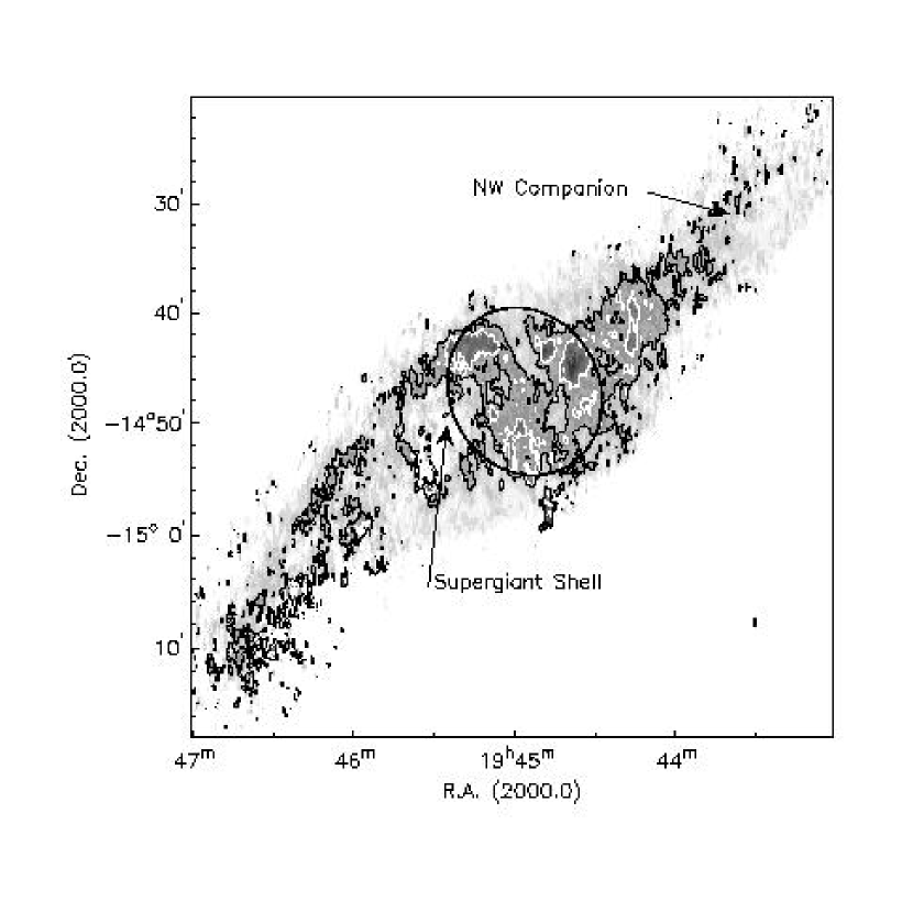
Figure 1.— Second moment map derived from the Hi data cube. Grayscales run from 5 $\,\mbox{km}\,\mbox{s}^{-1}$ (white) to 15 $\,\mbox{km}\,\mbox{s}^{-1}$ (black). The maximum values occuring in this map is 18.3 $\,\mbox{km}\,\mbox{s}^{-1}$. The black contour indicates 8 $\,\mbox{km}\,\mbox{s}^{-1}$. The white contour indicates 10 $\,\mbox{km}\,\mbox{s}^{-1}$. Here the entire data set has been used, and no attempt has been made to correct for e.g. the presence of high-velocity gas or asymmetric profiles. The beam of $42.4^{\prime\prime}\times 12^{\prime\prime}$ is indicated in the lower-right corner. For orientation, the large central ellipse indicates the approximate $R_{25}$ extent as given in the RC3. This defines the conventional optical extent of NGC 6822.

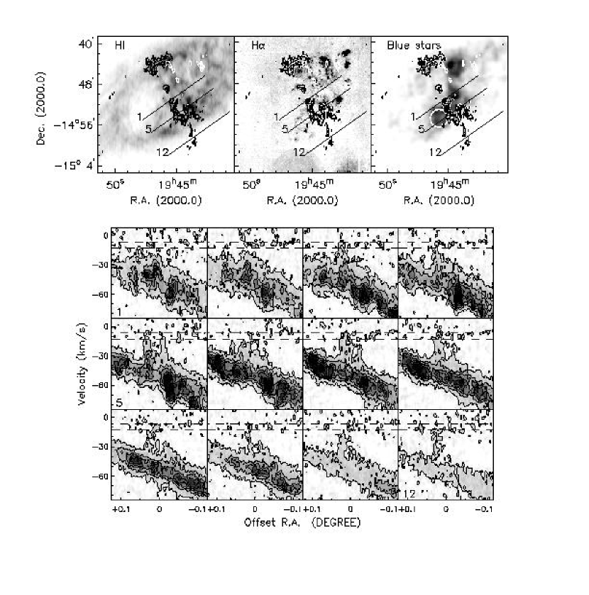
Figure 2.— High-velocity gas in NGC 6822. The top panels show the location of all gas deviating more than $18$ $\,\mbox{km}\,\mbox{s}^{-1}$ from the rotation velocity. Black contours indicate positive deviation, white contours negative deviation. The top-left panel shows the HV gas superimposed on the total Hi map. The top-centre panel shows the HV gas superimposed on the H$\alpha$ map. The top-right shows the HVC component superimposed on the surface density of blue stars. The location of the Blue Plume (see text) has been indicated with the white circle. The bottom mosaic shows position-velocity slices along the lines indicated in the top panels. The top-left slice corresponds with line 1, the bottom-right one with line 12. The intermediate slices are equally spaced between these two limits. Slices are integrated over 12^′′ and have a position angle of $125^{\circ}$. The horizontal dashed lines in the position-velocity diagrams indicate velocities with possible Galactic contamination. The lowest contour level is $2\sigma$, and contours increase in steps of $4\sigma$.

Figure 3.— Comparison of the quality of one- and two-component Gaussian fits to the Hi velocity profiles. Filled black dots indicate the positions where a two-component fit is preferred. The open circles indicate profiles where a one-component fit is preferred. The grey circles show the positions where one- and two-component fits perform equally well. The preference for one-component fits in the tidal arm is an artefact of residual galactic emission affecting the two-component fits. Offsets are with respect to position $(\alpha,\delta)=(19^{h}44^{m}09^{s},-14^{\circ}50^{m}54.0^{s}$).

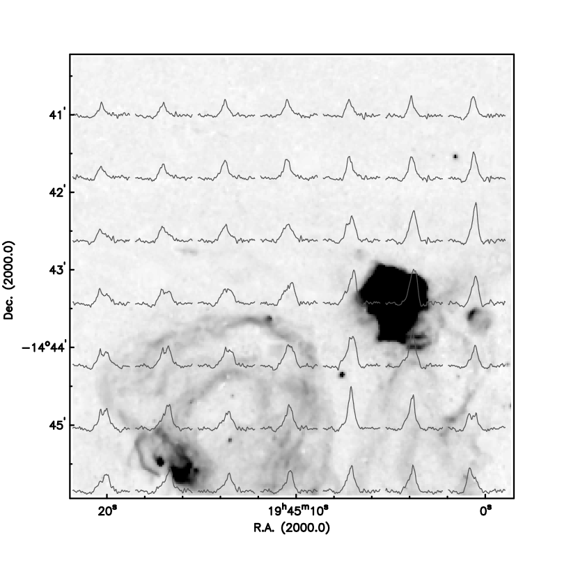
Figure 4.— Examples of Hi profiles. Their position in the diagram corresponds with their position on the sky. For comparison the corresponding local H$\alpha$ emission is shown as a grayscale background image. Profiles are plotted from -126 (left) to +35 (right) $\,\mbox{km}\,\mbox{s}^{-1}$.

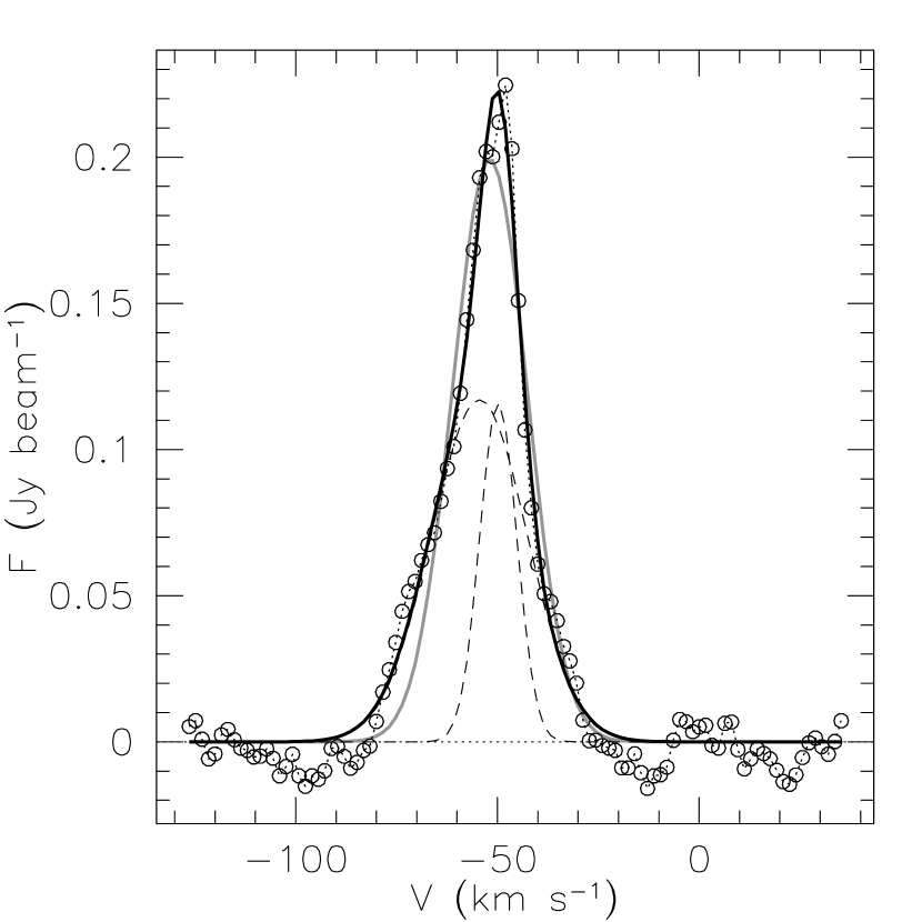
Figure 5.— Example of a non-Gaussian profile, at position ($\alpha$, $\delta$) = (19^h46^m05.25^s, $-14^{\circ}$45^′10.4^′′). Open circles represent the data, the grey thick line a one-component Gaussian fit, the black thick line a two-component Gaussiaun fit. The individual components are shown are thin dashed curves. The broad component has a dispersion of 11.9 $\,\mbox{km}\,\mbox{s}^{-1}$, the narrow component a dispersion of 4.6 $\,\mbox{km}\,\mbox{s}^{-1}$.

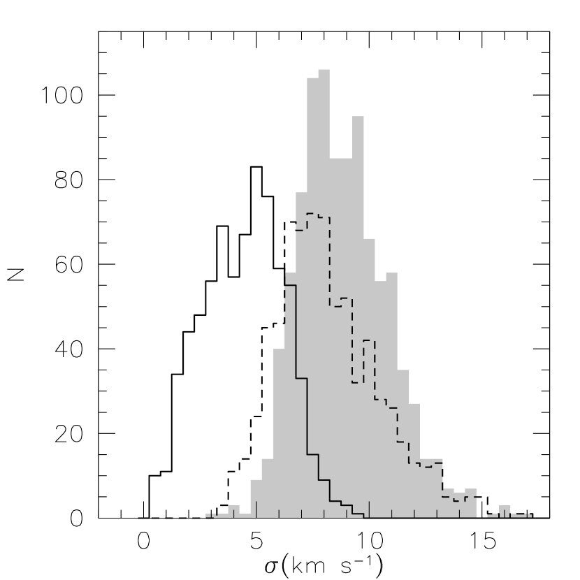
Figure 6.— Histogram of the dispersions derived from the one-component Gaussian fits (grey histogram) and from the two-component fit, with the broad component shown as the dashed-line histogram and the narrow component as the full-line histogram.

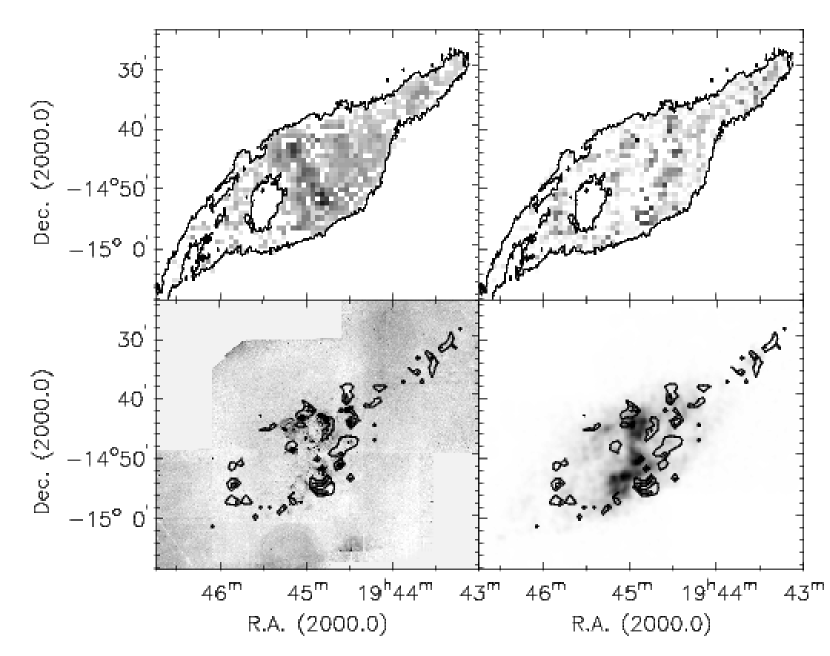
Figure 7.— Distribution of the cool and warm neutral components of the ISM. The top-left panel shows the distribution of the warm, broad-dispersion component, with the grayscale running from 0 to $3.2\cdot 10^{21}$ cm^-2. The contour shows the $5\cdot 10^{20}$ cm^-2 level of the total Hi column density distribution. The top-right panel shows the distribution of the cool narrow-linewidth component. The grayscale runs from 0 to $1.7\cdot 10^{21}$ cm^-2. The contour again shows the $5\cdot 10^{20}$ cm^-2 level of the total Hi column density distribution. The bottom left panel compares the distribution of the cool component (contours) with that of the H$\alpha$ (grayscale). The bottom-right panel shows the distribution of the cool component as contours overplotted on the surface density of the blue stars. For clarity we only show the peaks in the cool-component column density. In the bottom panels the contours start at $4\cdot 10^{20}$ cm^-2 and increase in steps of $5\cdot 10^{20}$ cm^-2.

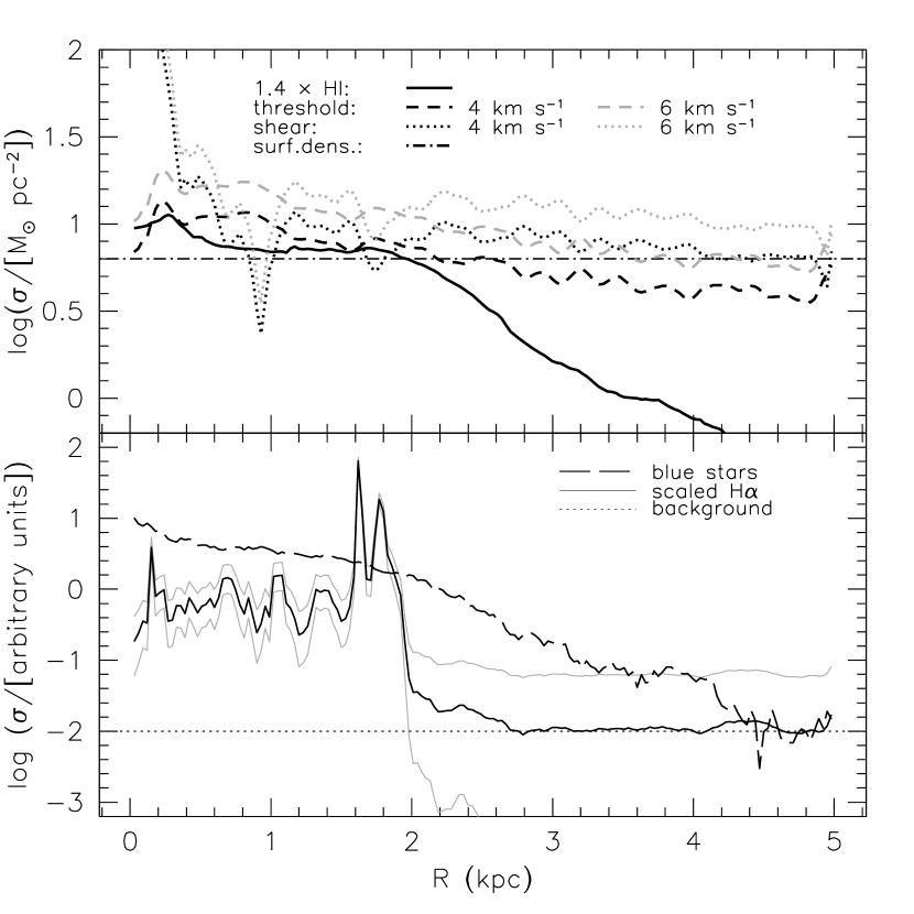
Figure 8.— Comparison of the radial distributions of star-formation threshold related properties. In the top panel, the full line shows the gas surface density (corrected for helium and inclination). The dotted lines shows the critical density derived using the Schaye (2004) version of the Hunter et al. (1998) critical density. The dashed lines show the Kennicutt (1989) critical densities. The grey critical density curves assume $\sigma=6$ $\,\mbox{km}\,\mbox{s}^{-1}$, the black critical density curves assume $\sigma=4$ $\,\mbox{km}\,\mbox{s}^{-1}$. The dash-dotted line indicates the Schaye (2004) critical density $\log(N_{H})=20.75$ (corrected for helium). The bottom panel shows the radial distribution of H$\alpha$ (with the 1$\sigma$ uncertainty due to noise in the sky background indicated by the gray lines) and blue star density. The normalized background levels are also indicated.

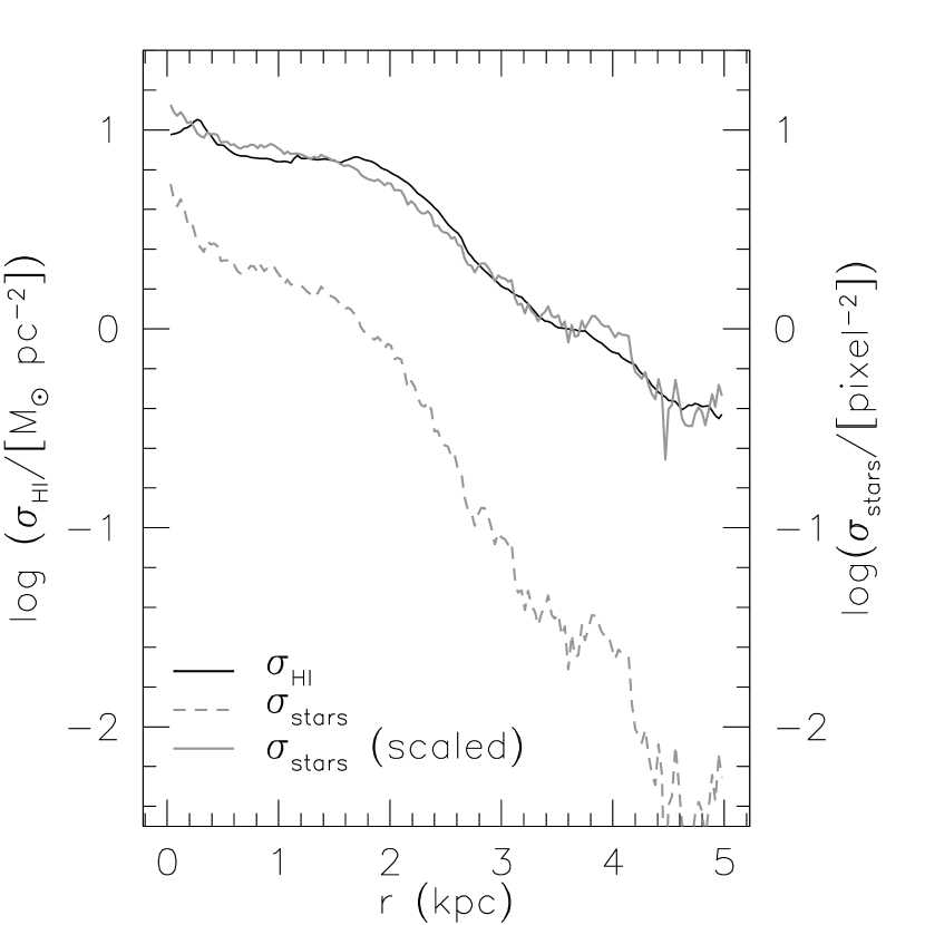
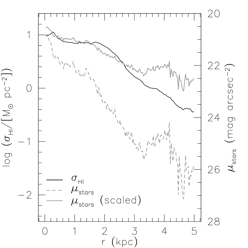
Figure 9.— Comparison of the surface densities of gas and blue stars. The left panel shows the inclination-corrected gas surface density (also corrected for helium) as the black line. The dashed grey curve shows the logarithmic radial surface density of blue stars, also corrected for inclination. The full grey curve shows the scaled stellar surface density using a scaling $\log(\sigma_{\rm stars}^{\rm scaled})=0.49\log(\sigma_{\rm stars})+0.77$. The RMS scatter of the scaled stellar curve with respect to the gas curve is 0.067 in $\log\sigma$. The right panel shows a similar relation between the gas surface density and the inclination-corrected surface brightness of the blue stars. The black curve again shows the logarithmic gas surface density. The dashed curve shows the radial surface brightness profile of the blue stars (with the scale along the righthand axis). The grey full curve shows the scaled surface brightness curve $\log(\sigma_{\rm stars}^{\rm scaled})=-0.19\cdot\mu_{\rm stars}+5.1$. Here only radii $R<3$ kpc were used for the scaling.

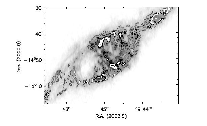
Figure 10.— Comparison of the two-dimensional Kennicutt (1989) star formation thresholds. The grayscale image shows the total Hi map. The contours enclose the regions predicted to be unstable to star formation. Various assumptions for the velocity dispersion are shown. The white contours have been computed using the variable dispersion as shown in the second-moment map. The black contours enclose the unstable regions computed assuming a constant dispersion of 6 $\,\mbox{km}\,\mbox{s}^{-1}$. The grey contours enclose the unstable regions computed using a dispersion of 4 $\,\mbox{km}\,\mbox{s}^{-1}$.

Figure 11.— Comparison of the various local star formation threshold predictions. The left column shows predictions for a $\sigma=6$ $\,\mbox{km}\,\mbox{s}^{-1}$ Toomre-$Q$ threshold. The black contour encloses unstable $\Sigma_{g}/\Sigma_{c}\geq 1$ regions. The black contour in the right column shows the prediction for a Toomre-$Q$ threshold assuming $\sigma=4$ $\,\mbox{km}\,\mbox{s}^{-1}$. The grey contour in the right column shows the critical Schaye (2004) surface density $\log(N_{HI})=20.75$. The top row compares the predictions with the total Hi distribution (grayscales). The centre panels compare with the H$\alpha$ distribution, the bottom panels with the blue star surface density distribution (both in grayscales). Note the good correspondence between the surface density and the Toomre-$Q$ predictions in the right-hand column.

Figure 12.— Pixel-to-pixel correlations. The left panel shows the correlation between H$\alpha$ and Hi surface density. The arrow indicates the $\log(N_{HI})=20.75$ level (corrected for inclination) with the associated uncertainty, as described in Schaye (2004). The full horizontal line indicates the average background level, the dotted lines the 1$\sigma$ noise in the background level. The centre panel shows the correlation between H$\alpha$ intensity and $\Sigma_{g}/\Sigma_{c}$. Lines are as in the top-left panel. The right panel shows the correlation between Hi column density and critical density $\Sigma_{c}$.

References

- Allen (2001) Allen, R. J. 2001, ASP Conf. Ser. 240: Gas and Galaxy Evolution, 240, 331
- Billett et al. (2002) Billett, O. H., Hunter, D. A., & Elmegreen, B. G. 2002, AJ, 123, 1454
- de Blok & Walter (2000) de Blok, W. J. G. & Walter, F. 2000, ApJ, 537, L95
- de Blok & Walter (2005) de Blok, W. J. G. & Walter, F. 2005, in preparation
- Elmegreen (2002) Elmegreen, B. G. 2002, ApJ, 577, 206
- Elmegreen & Parravano (1994) Elmegreen, B. G., & Parravano, A. 1994, ApJ, 435, L121
- Ferguson et al. (1998) Ferguson, A. M. N., Wyse, R. F. G., Gallagher, J. S., & Hunter, D. A. 1998, ApJ, 506, L19
- Gerritsen & Icke (1997) Gerritsen, J. P. E., & Icke, V. 1997, A&A, 325, 972
- Gil de Paz et al. (2005) Gil de Paz, A., et al. 2005, ApJ, 627, L29
- Hunter et al. (1998) Hunter, D. A., Elmegreen, B. G., & Baker, A. L. 1998, ApJ, 493, 595
- Hunter et al. (2001) Hunter, D. A., Elmegreen, B. G., & van Woerden, H. 2001, ApJ, 556, 773
- Kennicutt (1989) Kennicutt, R. C. 1989, ApJ, 344, 685
- Martin & Kennicutt (2001) Martin, C. L., & Kennicutt, R. C. 2001, ApJ, 555, 301
- Parodi & Binggeli (2003) Parodi, B.R., & Binggeli, B. 2003, A&A, 398, 501
- Quirk (1972) Quirk, W. J. 1972, ApJ, 176, L9
- Schaye (2004) Schaye, J. 2004, ApJ, 609, 667
- Skillman (1987) Skillman, E.D. 1987, in Star Formation in Galaxies, edited by C.J. Lonsdale Persson (NASA Conf. Pub. CP-2466), p. 263
- Taylor & Webster (2005) Taylor, E.N., Webster, R.L. 2005, ApJ, in press (astro-ph/0501514)
- Thilker et al. (2005) Thilker, D. A., et al. 2005, ApJ, 619, L79
- van der Hulst et al. (1993) van der Hulst, J. M., Skillman, E. D., Smith, T. R., Bothun, G. D., McGaugh, S. S., & de Blok, W. J. G. 1993, AJ, 106, 548
- Weldrake et al. (2003) Weldrake, D. T. F., de Blok, W. J. G., & Walter, F. 2003, MNRAS, 340, 12
- Young & Lo (1997) Young, L. M., & Lo, K. Y. 1997, ApJ, 490, 710
- Young & Lo (1996) Young, L. M., & Lo, K. Y. 1996, ApJ, 462, 203