Observational Constraints on Silent Quartessence

Abstract

We derive new constraints set by SNIa experiments (‘gold’ data sample of Riess et al.), X-ray galaxy cluster data (Allen et al. Chandra measurements of the X-ray gas mass fraction in 26 clusters), large scale structure (Sloan Digital Sky Survey spectrum) and cosmic microwave background (WMAP) on the quartessence Chaplygin model. We consider both adiabatic perturbations and intrinsic non-adiabatic perturbations such that the effective sound speed vanishes (Silent Chaplygin). We show that for the adiabatic case, only models with equation of state parameter $|\alpha|\lesssim 10^{-2}$ are allowed: this means that the allowed models are very close to $\Lambda$CDM. In the Silent case, however, the results are consistent with observations in a much broader range, $-0.3<\alpha<0.7$.

I Introduction

Two of the major puzzles of contemporary cosmology are the nature of dark matter and of dark energy, the two big players in the cosmic arena. So far, the only knowledge of these components refers to their density fraction and to their equation of state, and even on these numbers we still have a large uncertainty. Greater still is the ignorance of their clustering properties: although we assume that essentially all the dark matter clusters in observable objects and all the dark energy does remain quite homogeneous, this is to a large extent only a simplification rather a consequence of observations.

It is therefore no surprise that many works are currently devoted to the possibility of merging the two puzzles into a single one: that is, finding a single origin for both dark matter and dark energy. A possibility is to assume an interaction between dark matter and dark energy ame or to fit both into a single complex field maibon . However, these models still contain two separate fields that account ultimately for the two components. On a different level lies the hypothesis that there is a single fluid that behaves as dark matter or dark energy according to the background or the local density. Since there is only one unifying dark-matter-energy component, besides baryons, photons and neutrinos, this model is usually referred to as quartessence mak03a . A phenomenological prototype of quartessence models is the generalized Chaplygin model kam ; bil ; ben , an exotic fluid with an inverse power law homogeneous equation of state (EOS), $\overline{p}=-M^{4(\alpha+1)}/\overline{\rho}^{\alpha}$, where $M$ has dimension of mass and $\alpha>-1$ is a dimensionless parameter ($\alpha=1$ is the original Chaplygin gas). Such equation of state leads to a component which behaves as dust in the past and as cosmological constant in the future. For $\alpha=0$ the model reduces to $\Lambda$CDM ave03 .

For a wide range of values of the parameter $\alpha$, the quartessence Chaplygin model is compatible with several cosmological tests that involve only the background metric mak03b . Nevertheless, problems may occur when one considers perturbations. For instance, the CMB anisotropies spectrum is strongly suppressed with respect to $\Lambda\mathrm{CDM}$ CF . Further, it was shown that, unless $\alpha$ is very much close to $\alpha=0$, the mass power spectrum presents strong instabilities and oscillations sand . A quantitative CMB analysis afbc (see also BD for a pre-WMAP analysis of the generalized Chaplygin gas as dark energy) found that the parameter $\alpha$ should be small ($\alpha<0.2$ at 95% CL), even including an additional CDM component, and smaller still without the latter. We will show below that in fact this limit reduces to $|\alpha|<0.01$. It is clear that this strong limit is due to the finite sound speed of the Chaplygin fluid: when it is sufficiently large and positive, it prevents clustering on small scales and therefore introduces a cut in the power spectrum which is at odds with observations; when it is negative, on the other hand, the clustering at small scales is enhanced beyond control.

It is important to stress, however, that unlike the background tests, the perturbation analysis need further assumptions beyond the equation of state. In reis03b , it was shown that it is possible to avoid the mass power spectrum problem if, for instance, pressure perturbation vanishes. This can be done by introducing a special type of intrinsic entropy perturbation such that the effective sound speed hu of the cosmic fluid vanishes (we denote this as silent perturbations). We call the Chaplygin quartessence model with vanishing pressure perturbation Silent Chaplygin and refer to the standard case as adiabatic Chaplygin.

The main goal of this paper is to show that, unlike adiabatic Chaplygin, Silent Chaplygin is consistent with CMB data for a wide range of parameters. Besides CMB, we also consider consistency of Silent Chaplygin with current data from large scale structure, from type Ia supernovae (SNIa) and baryon fraction in galaxy clusters. Using the latest data sets, we review all these tests using a careful treatment, presenting the outcome of a combined analysis of the data for both Silent and adiabatic Chaplygin.

II Basic equations

In this section we give a brief and basic description of the model. The conservation equation for the generalized Chaplygin gas component in a Robertson-Walker metric is solved by

$$\overline{\rho}_{Ch}=\overline{\rho}_{Ch0}[-w_{0}+\frac{1+w_{0}}{a^{3(\alpha+1)}}]^{\frac{1}{1+\alpha}},$$ (1)

where $a$ is the scale factor ($a=1$ today) and $w_{0}=-\frac{M^{4}}{\overline{\rho}_{Ch0}^{\alpha+1}}$ is the present equation of state.

The equation-of-state parameter ($w=\overline{p}/\overline{\rho}$) and the adiabatic sound velocity ($c_{s}^{2}=d\overline{p}/d\overline{\rho}$) for the Chaplygin gas, are given by

$$w_{Ch}(a)=\frac{w_{0}}{-w_{0}+(1+w_{0}){a^{-3(\alpha+1)}}}$$ (2)

and

$$c_{sCh}^{2}(a)=-\alpha\,w_{Ch}(a).$$ (3)

From the equation above, it is clear that at early times, when $a\rightarrow 0,$ we have $w_{Ch}\rightarrow 0$, and the fluid behaves as non relativistic matter. At late times, when $a\gg 1$, we obtain $w_{Ch}\rightarrow-1$. Further, the adiabatic sound speed has maximum value when the equation of state parameter is minimum. Therefore, the epoch of cosmic acceleration, in these models, coincides with that of large $c_{s}^{2}$. As remarked in reis05 , this is a characteristic of all unified models in which the equation of state is convex, i.e., is such that $\frac{d^{2}\overline{p}}{d\overline{\rho}^{2}}=\frac{dc_{s}^{2}}{d\overline{\rho}}<0$. However, this property is not mandatory for a general fluid. Models with concavity changing equations of state, may have $c_{s}^{2}$ negligibly small when the energy density reaches its minimum value. This is an important property that must be considered in constructing acceptable adiabatic quartessence models makler05 .

The perturbation equations for a fluid with equation of state $w$ and adiabatic sound speed $c_{s}^{2}$ in synchronous gauge are (for the sake of simplicity, here we neglect baryons and radiation, and we assume that both spatial curvature and the anisotropic perturbation vanish)

$$\delta^{\prime}=-3(w\Gamma+c_{s}^{2}\delta-w\delta)-(1+w)(\theta+\frac{h_{L}^{\prime}}{2})$$ (4)

$$\theta^{\prime}=\frac{k^{2}}{(1+w)\mathcal{H}^{2}}(w\Gamma+c_{s}^{2}\delta)+(3c_{s}^{2}-1-\frac{\mathcal{H}^{\prime}}{\mathcal{H}})\theta$$ (5)

$$h_{L}^{\prime}=\frac{2k^{2}\eta}{{}^{\mathcal{H}^{2}}}+3\delta\Omega$$ (6)

$$\eta^{\prime}=\frac{3(1+w)\mathcal{H}^{2}\theta\Omega}{2k^{2}}$$ (7)

where derivatives are with respect to $\log a$. Here $\delta$ is the density contrast, $\Omega$ is the density parameter, $h_{L}$ and $\eta$ are metric perturbations, $\theta$ is the divergence of the velocity perturbation, $\Gamma$ is the entropy perturbation and $\mathcal{H}\equiv da/d\tau$, $\tau$ being the conformal time. To these equations, we must add the equations for baryons and relativistic fluid. The assumption of a silent universe requires that reis03b

$$\delta p=\overline{p}\Gamma+c_{s}^{2}(\delta\rho)=0$$

so that

$$\Gamma=-\frac{c_{s}^{2}}{w}\delta$$

We adopt therefore these equations with $w=w_{Ch}$ and $c_{s}=c_{sCh}$. With this choice, $\Gamma=\alpha\delta$ and models with $\alpha=0$ are both, silent and adiabatic.

III Observational constraints

In the subsections below, we will derive constraints on the parameters $\alpha$ and $w_{0}$ from four data sets: SNIa, X-ray cluster gas fraction, SDSS power spectrum and CMB.

III.1 SNIa

The luminosity distance of a light source is defined in such a way as to generalize to an expanding and curved space the inverse-square law of brightness valid in a static Euclidean space,

$$d_{L}=\left(\frac{L}{4\pi\mathcal{F}}\right)^{1/2}.$$ (8)

In Eq. (8), ${L}$ is the absolute luminosity and $\mathcal{F}$ is the measured flux.

For a source of absolute magnitude $M$, the apparent bolometric magnitude $m(z)$ can be expressed as

$$m(z)= M-5\log H_{0}+25+5\log D_{L}$$

$$= M+42.3841-5\log h\,+5\log D_{L},$$ (9)

where $D_{L}$ is the luminosity distance in units of $H_{0}^{-1}$(we are using $c=1$),

$$D_{L}=\int_{0}^{z}\left[E\left(z^{\prime}\right)\right]^{-1}dz^{\prime}\,,$$ (10)

where

$$E^{2}\left(z\right)=\left\{\omega_{b}h^{-2}\left(1+z\right)^{3}\right.$$

$$+\left.(1-\omega_{b}h^{-2})\left[-w_{0}+(1+w_{0})\left(1+z\right)^{3\left(1+\alpha\right)}\right]^{\frac{1}{(1+\alpha)}}\right\}.$$ (11)

Here, $z$ is the redshift, $\omega_{b}=\Omega_{b}h^{2}$, and $h$ is the Hubble constant in units of $100km/sMpc^{-1}$.

For the SNIa analysis, we use the ‘gold’ data set of Riess et al. riess04 . The data in this sample is given in terms of the extinction corrected distance modulus, $\mu_{0}=m-M$. To obtain the likelihood of the parameters, we use a $\chi^{2}$ statistics such that,

$$\chi^{2}(\alpha,w_{0},h,\omega_{b})=$$

$$\sum\limits_{i=1}^{157}\left(\frac{\mu_{0,i}-42.3841+5\log h\,-5\log D_{L}(z_{i,}\alpha,w_{0},h,\omega_{b})}{\sigma_{\mu_{0,i}}}\right)^{2}.$$ (12)

In (12), $\sigma_{\mu_{0,i}}$ are the estimated errors in the individual distance moduli, including uncertainties in galaxy redshift and also taking into account the dispersion in supernovae redshift due to peculiar velocities (see riess04 for details). To determine the likelihood of the parameters $\alpha$ and $w_{0}$, we marginalize the likelihood function over $h$ and $\omega_{b}$. We use two different priors in this work. We consider flat priors when combining the SNIa and clusters results with CMB, while in this and in the next subsection we adopt Gaussian priors such that $h=0.72\pm 0.08$ hst and $\omega_{b}=0.0214\pm 0.002$ kir03 . The results of our SNIa analysis are displayed in Fig. 1. In the figure, we show $68\%$ and $95\%$ confidence level contours in the $(\alpha,$ $w_{0})$ plane.

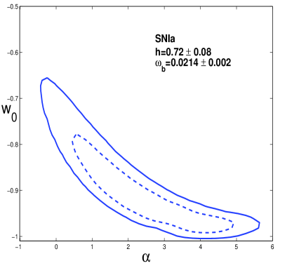
Figure 1: Constant confidence contours ($68\%$ and $95\%$) in the ($\alpha,w_{0}$) plane allowed by SNIa data, as described in the text

III.2 X-ray Cluster Gas Fraction

Clusters of galaxies are the most recent large-scale structures formed and the largest gravitationally bound systems known. Therefore, the determination of their matter contents is important since cluster properties should approach those of the Universe as a whole. By measuring the baryon mass fraction $\Omega_{b}/\Omega_{m}$ in rich clusters, and combining this ratio with $\Omega_{b}$ determinations from primordial nucleosynthesis, constraints on $\Omega_{m}$ can be placed white . Further, by assuming that baryon mass fraction in clusters of galaxies is independent of redshift, it is also possible to constrain the geometry and, consequently, the dark energy density. A method based on this idea was suggested by Sasaki sasaki and Pen pen and further developed and applied by Allen, Schmidt, and Fabian allen02 .

In this section we use the new data set of Allen et al. allen04 to constraint the Chaplygin models. These authors extracted from Chandra observations the x-ray gas mass fraction ($f_{\text{gas}}$) of twenty six massive, dynamically relaxed galaxy clusters, with redshifts in the range $0.08<z<0.9$, and that have converging $f_{\text{gas}}$ within a radius $r_{2500}$ (radius encompassing a region with mean mass density $2500$ times the critical density of the Universe at the cluster redshift).

To determine the confidence region of the parameters of the model, we use the following $\chi^{2}$ function in our computation:

$$\chi^{2}(\alpha,w_{0},h,\omega_{b},b)=\sum\limits_{i=1}^{26}\frac{\left[f_{\text{gas}}^{\text{mod}}(z_{i},\alpha,w_{0},h,\omega_{b},b)-f_{\text{gas},i}\right]^{2}}{\sigma_{f_{\text{gas},i}}^{2}}\,,$$ (13)

where $z_{i}$, $f_{\text{gas},i}$, and $\sigma_{f_{\text{gas},i}}$ are, respectively, the redshifts, the SCDM ($h=0.5$) best-fitting values, and the symmetric root-mean-square errors for the 26 clusters as given in allen04 . In Eq. (13), $f_{\text{gas}}^{\text{mod}}$ is the model function allen02

$$f_{\text{gas}}^{\text{mod}}=\frac{b\omega_{b}h^{-2}}{(1+0.19\sqrt{h})\Omega_{m}^{\text{eff}}}\left(\frac{h}{0.5}\frac{d_{A}^{\text{EdS}}}{d_{A}^{\alpha,A}}\right)^{3/2}\,.$$ (14)

Here, $d_{A}=(1+z)^{-2}d_{L}$ is the angular diameter distance to the cluster, $b$ is a bias factor that takes into account the fact that the baryon fraction in clusters could be lower than for the Universe as a whole and

$$\Omega_{m}^{\text{eff}}=(1-\omega_{b}h^{-2})\left(1+w_{0}\right)^{1/\left(1+\alpha\right)}+\omega_{b}h^{-2}\,.$$ (15)

is the effective matter density parameter mak03b . In our computations, we first marginalize analytically over the bias factor assuming that it is Gaussian-distributed with $b=0.824\pm 0.089$ allen04 ; rapetti . To determine the likelihood of the parameters $\alpha$ and $w_{0}$, we next marginalize the likelihood function over $h$ and $\omega_{b}$. As remarked before, we assume here a Gaussian prior such that $h=0.72\pm 0.08$ hst and $\omega_{b}=0.0214\pm 0.002$ kir03 .

In Fig. 2, we show the $68\%$ and $95\%$ confidence contours on the parameters $\alpha$ and $w_{0}$ determined from the Chandra data.

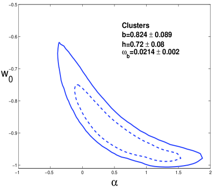
Figure 2: Constant confidence contours ($68\%$ and $95\%$) in the ($\alpha,w_{0}$) plane from cluster $f_{gas}$ data as described in the text.

III.3 CMB

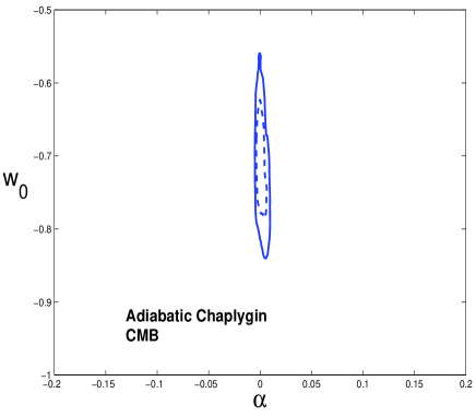
Figure 3: Constant confidence contours ($68\%$ and $95\%$) in the ($\alpha,w_{0}$) plane allowed by CMB, as described in the text.

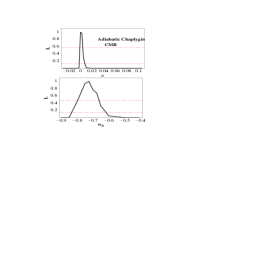
Figure 4: CMB likelihood functions for $\alpha$ and $w_{0}$ in the adiabatic case. The horizontal lines mark the 68$\%$ and 95$\%$ c.l., top to bottom.

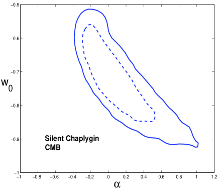
Figure 5: Constant confidence contours ($68\%$ and $95\%$) in the ($\alpha,w_{0}$) plane allowed by CMB, as described in the text

Here we compare the model to the combined temperature and polarization power spectrum estimated by WMAP hin . To derive the likelihood we adopt a version of the routine described in Verde et al. verde , which takes into account all the relevant experimental properties (calibration, beam uncertainties, window functions, etc).

Our theoretical model depends on two Chaplygin parameters, four cosmological parameters and the overall normalization $N$:

$$\alpha,w_{0},n_{s},h,\omega_{b},\tau,N.$$ (16)

The overall normalization has been integrated out numerically. We calculate the theoretical $C_{\ell,t}$ spectra by a modified parallelized CMBFAST sel code that includes the full set of perturbation equations CF ; afbc with the addition of non-adiabatic pressure perturbations. We do not include gravitational waves and the other parameters are set as follows: $T_{cmb}=2.726K,$ $Y_{He}=0.24,N_{\nu}=3.04$.

We evaluated the likelihood on a unequally spaced grid of roughly $50,000$ models (for each normalization) with the following top-hat broad priors: $w_{0}\in(-1,-0.5),$ $\quad\alpha\in(-0.8,1.5),\quad$ $n_{s}\in(0.8,1.2),$ $\quad\omega_{b}\in(0.02,0.025),\quad$ $\tau\in(0.,0.3)$. For the Hubble constant we adopted the top-hat prior $h\in(0.6,0.8);$ we also employed the HST result hst $h=0.72\pm 0.08$ (Gaussian prior).

In Fig. 3, we show the confidence region on $\alpha,w_{0}$ in the adiabatic case, after marginalization over all the other parameters with flat priors: as it can be seen, this is the most stringent test among those studied in this paper. As anticipated, it restricts $\alpha$ to be very close to 0: in other words, observations of CMB demands that the background of adiabatic Chaplygin be almost indistinguishable from $\Lambda$CDM. In Fig. 5 we contrast this result with the silent case: now the allowed region for $\alpha$ widens a lot, encompassing values close to unity. What is particularly interesting is that even with $\alpha=1$, Silent Chaplygin is consistent at the 2$\sigma$ level, while it was obviously ruled out in the adiabatic case. In Figs. 4 and 6. we show the one-dimensional likelihood for $\alpha$ and $w_{0}$, with marginalization over all the other parameters.

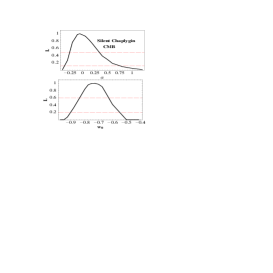
Figure 6: CMB likelihood functions for $\alpha$ and $w_{0}$ in the silent case. The horizontal lines mark the 68$\%$ and 95$\%$ c.l., top to bottom.

III.4 Large scale structure

The results of Sandvik et al. (2004) sand have shown that the matter power spectrum of adiabatic Chaplygin is plagued by strong instabilities and oscillations for any $\alpha$ significantly different from zero, leading to a stringent upper limit to $|\alpha|$. In reis03b , it has been shown that these problems do not occur for the silent model. To test this in a more quantitative way we perform here a simplified likelihood analysis with the following procedure. We compared the baryon spectra of the silent case to the matter power spectrum of Sloan Digital Sky Survey (SDSS) as obtained in Tegmark et al. (2004) teg04 , cutting at $k=0.02h/$Mpc, using the likelihood routine provided by M. Tegmark tegweb , and marginalizing over the amplitude (i.e., we are comparing only the slope of the spectrum, not its absolute value). In order to save computer time we restricted ourselves to a subset of parameters, fixing $\omega_{b}=0.023$, $n_{s}=1$ and $h=0.7$. As we show in Fig. 7, the results are rather similar to the CMB case. Since we used only a very small subset of the whole parameters space we will not include the SDSS likelihood in the combined likelihood of the next section. The loss in constraining power is acceptable since one can easily see that the CMB and the SDSS confidence regions are overlapping to a good extent. Moreover, extending the range of parameters as in the CMB case the SDSS constraints would become weaker and would not add much to the information from the CMB.

We also calculated the baryon fluctuation variance $\sigma_{8}$ (i.e. the absolute normalization of the spectrum) for the same subset of parameters. In Fig. 8 we show the contour plots of the likelihood assuming a Gaussian distribution of the observed $\sigma_{8}$ with $\sigma_{8}=0.9\pm 0.1$. This test is meant to be only qualitative since the value of $\sigma_{8}$ that is derived from data is strongly degenerate with $\Omega_{m}$ and with the bias factor and/or it depends on calibration obtained with $N$-body simulations based on some specific cosmological model. We only notice that for the Silent Chaplygin case there exists a large region in our parameter space which accounts for values of $\sigma_{8}$ which are consistent with the standard estimation. It is nevertheless interesting to note that the $\sigma_{8}$ analysis shows preference for lower values of $w_{0}$ (for a fixed $\alpha$) than the CMB test. This could help to further reduce the parameters space.

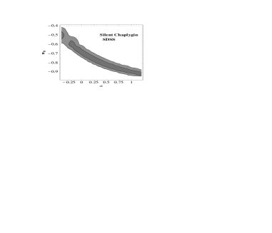
Figure 7: SDSS likelihood functions at 68$\%$ and 95 $\%$ c.l. for $\alpha$ and $w_{0}$ in the silent case.

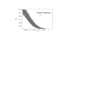
Figure 8: Likelihood function for $\sigma_{8}$ at 68$\%$ and 95 $\%$ c.l. for $\alpha$ and $w_{0}$ in the silent case.

IV Combined Constraints and Conclusion

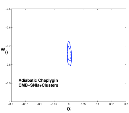
Figure 9: Constant confidence contours ($68\%$ and $95\%$) in the ($\alpha,w_{0}$) plane allowed by SNIa, clusters and CMB, as described in the text.

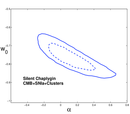
Figure 10: Constant confidence contours ($68\%$ and $95\%$) in the ($\alpha,w_{0}$) plane allowed by SNIa, clusters and CMB, as described in the text

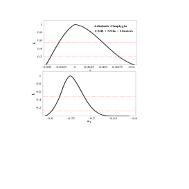
Figure 11: Likelihood functions for $\alpha$ and $w_{0}$ in the adiabatic case for SNIa, clusters and CMB. The horizontal lines mark the 68$\%$ and 95$\%$ c.l., top to bottom.

Figure 12: Likelihood functions for $\alpha$ and $w_{0}$ in the silent case for SNIa, clusters and CMB. The horizontal lines mark the 68$\%$ and 95$\%$ c.l., top to bottom. For comparison, we plot as dotted lines the combined likelihood functions of the adiabatic case.

Here we present a combined analysis of the constraints discussed in the previous section. In Fig. 9 we display the allowed region of the parameters $w_{0}$ and $\alpha$ from a combination of data from SNIa, clusters and CMB in adiabatic Chaplygin. The constraints on the parameter $\alpha$ are roughly the same as those obtained from CMB alone. Only models with $\alpha$ very close to the $\Lambda$CDM limit are allowed. Although including SNIa and clusters in the CMB analysis almost do not affect the constraints on $\alpha$, they tighten the constraints on the parameter $w_{0}$, reducing even more the allowed region of the parameters space in the adiabatic case. The final result (95% c.l.) for the adiabatic case is

$$-0.005<\alpha<.01,\quad-0.8<w_{0}<-0.7.$$ (17)

In contrast, in Fig. 10, the Silent Chaplygin model is consistent with the observables considered here for a wide range of parameters. The constraints in the silent case are (95% c.l.)

$$-0.25<\alpha<0.5,\quad-0.87<w_{0}<-0.68,$$ (18)

with a remarkable fifty-fold extension in the range of $\alpha$. The one-dimensional likelihood functions are shown in Figs. 11 and 12.

The idea of unifying dark matter and dark energy through a single component has motivated many works in the last few years. Most of these investigations concentrated their efforts in analyzing the generalized Chaplygin fluid, that is considered the prototype of the quartessence models. After the results of CF ; sand ; afbc , it became clear that adiabatic Chaplygin, as quartessence, is ruled out unless the parameter $\alpha$ is very close to zero. In the present paper we confirmed this result by using current CMB data, extending the quantitative results of afbc to quartessence models. In fact, for an effective sound speed different from zero, any quartessence model with a convex EOS will suffer the same kind of problem reis05 . There are two simple ways to get around this problem: choosing an EOS not convex makler05 or introducing entropic perturbations as we did in this paper. This shows that indeed quartesence models of the Chaplygin type (one fluid, two parameters) can be considered as real alternatives to $\Lambda$CDM (two fluids, one parameter). It is clear however that these phenomenological models should be further investigated: the challenge is to connect them to a more fundamental theory.

Finally, we remark that one possible source of problems for Silent Chaplygin is lensing skewness reis04 . It would be remarkable if higher-order or non-linear effects would prove necessary to rule out, or strongly constrain, these models.

- (1) L. Amendola, Phys. Rev. D 62, 043511, (2000).
- (2) R. Mainini & S.A. Bonometto, Phys. Rev. Lett. 93, 121301 (2004).
- (3) M. Makler, S.Q. Oliveira & I. Waga, Phys. Lett. B 555, 1 (2003).
- (4) A. Kamenshchik, U. Moschella & V. Pasquier, V., 2001, Phys. Lett. B 511, 265 (2001).
- (5) N. Bilić, G.B. Tupper & R.D. Viollier, Phys. Lett. B 535, 17 (2002).
- (6) M.C. Bento, O. Bertolami & A.A. Sen, Phys. Rev. D 66 , 043507 (2002).
- (7) P.P. Avelino, L.M.G. Beça, J.P.M. de Carvalho & C.J.A.P. Martins, JCAP 09, 002 (2003).
- (8) M. Makler, S.Q. Oliveira & I. Waga, Phys. Rev. D 64, 123521 (2003); A. Dev, D. Jain & J.S. Alcaniz, Astron. Astrophys. 417, 847 (2004); R. Colistete Jr. & J.C. Fabris, Class. Quant. Grav. 22, 2813 (2005); M.C. Bento, O. Bertolami, N.M.C. Santos, A.A. Sen, Phys. Rev. D 71, 063501 (2005).
- (9) D. Carturan & F. Finelli, Phys. Rev. D 68, 103501 (2003).
- (10) H. Sandvik, M. Tegmark, M. Zaldarriaga & I. Waga, Phys. Rev. D 69, 123524 (2004).
- (11) L. Amendola, F. Finelli, C. Burigana & D. Carturan, JCAP 07, 005 (2003).
- (12) R. Bean & O. Dore, Phys. Rev. D 68, 023515 (2003).
- (13) R.R.R. Reis, I. Waga, M.O. Calvão & S.E. Jorás, Phys. Rev. D 68, 061302(R) (2003).
- (14) W. Hu, Astrophys. J. 506, 485 (1998).
- (15) R.R.R. Reis, M. Makler & I. Waga, Class. Quant. Grav. 22, 353 (2005).
- (16) M. Makler, R. R. R. Reis, L. Amendola & I. Waga, in preparation
- (17) A.G. Riess et al., Astrophys. J. 607, 665 (2004).
- (18) W. Freedman et al., Astrophys. J. 553, 47 (2001).
- (19) D. Kirkman et al., Astrophys. J. Suppl., 149, 1 (2003).
- (20) S.D.M. White & C. S. Frenk, Astrophys. J. 379, 52 (1991); S.D.M. White, J.F. Navarro, A.E. Evrard & C. Frenk, Nature (London) 366, 429 (1993).
- (21) S. Sasaki, Publ. Astron. Soc. Jpn., 48, L119 (1996).
- (22) U. Pen, New Astronomy 2, 309 (1997).
- (23) S.W. Allen, R.W. Schmidt & A.C. Fabian, Mont. Not. R. Astron. Soc. 334, L11 (2002).
- (24) S.W. Allen et al., Mont. Not. R. Astron. Soc. 353, 457 (2004).
- (25) D. Rappeti, S.W. Allen & J. Weller, Mont. Not. R. Astron. Soc. 360, 555 (2005).
- (26) G. Hinshaw et al. [WMAP collaboration], Astrophys. J. Suppl. 148, 135 (2003).
- (27) L. Verde et al. [WMAP collaboration], Astrophys. J. Suppl. 148, 195 (2003).
- (28) M. Tegmark, et al. [the SDSS collaboration], Phys. Rev. D 69, 103501 (2004); M. Tegmark, et al. [the SDSS collaboration], Astrophys. J. 606, 702 (2004).
- (29) http://space.mit.edu/home/tegmark/sdss.html
- (30) U. Seljak & M. Zaldarriaga, Ap. J. 469, 437 (1996).
- (31) R.R.R. Reis, M. Makler & I. Waga, Phys. Rev. D 69, 101301(R) (2004).