Testing Primordial Non-Gaussianity in CMB Anisotropies

Abstract

Recent second-order perturbation computations have provided an accurate prediction for the primordial gravitational potential, $\Phi(\mathbf{x})$, in scenarios in which cosmological perturbations are generated either during or after inflation. This enables us to make realistic predictions for a non-Gaussian part of $\Phi(\mathbf{x})$, which is generically written in momentum space as a double convolution of its Gaussian part with a suitable kernel, $f_{\rm NL}(\mathbf{k}_{1},\mathbf{k}_{2})$. This kernel defines the amplitude and angular structure of the non-Gaussian signals and originates from the evolution of second-order perturbations after the generation of the curvature perturbation. We derive a generic formula for the CMB angular bispectrum with arbitrary $f_{\rm NL}(\mathbf{k}_{1},\mathbf{k}_{2})$, and examine the detectability of the primordial non-Gaussian signals from various scenarios such as single-field inflation, inhomogeneous reheating, and curvaton scenarios. Our results show that in the standard slow-roll inflation scenario the signal actually comes from the momentum-dependent part of $f_{\rm NL}(\mathbf{k}_{1},\mathbf{k}_{2})$, and thus it is important to include the momentum dependence in the data analysis. In the other scenarios the primordial non-Gaussianity is comparable to or larger than these post-inflationary effects. We find that WMAP cannot detect non-Gaussian signals generated by these models. Numerical calculations for $l>500$ are still computationally expensive, and we are not yet able to extend our calculations to Planck’s angular resolution; however, there is an encouraging trend which shows that Planck may be able to detect these non-Gaussian signals.

I Introduction

Inflation is a building-block of the standard model of modern cosmology. It is widely believed that there was an early stage in the history of the Universe – before the epoch of primordial nucleosynthesis – when the expansion rate of the Universe was accelerated. Such a period of cosmological inflation can be attained if the energy density of the Universe is dominated by the vacuum energy density associated with the potential of a scalar field, called the inflaton lrreview . Inflation has become so popular also because of another compelling feature. It provides a causal mechanism for the production of the first density perturbations in the early Universe which are the seeds for the Large-Scale Structure (LSS) of the Universe and for the Cosmic Microwave Background (CMB) temperature and polarization anisotropies that we observe today. In the inflationary picture, primordial density and gravity-wave fluctuations were created from quantum fluctuations and then left the horizon during an early period of superluminal expansion of the Universe, with the amplitude “frozen-in”. Perturbations at the surface of last scattering are observable as temperature and polarization anisotropies in the CMB. The inflationary paradigm has been tested carefully by the data of the Wilkinson Microwave Anisotropy Probe (WMAP) mission bennett/etal:2003b . The WMAP collaboration has produced a full-sky map of the angular variations of the CMB with unprecedented accuracy. The WMAP data confirm the inflationary mechanism as responsible for the generation of curvature (adiabatic) superhorizon fluctuations ex . Since the primordial cosmological perturbations are tiny, the generation and evolution of fluctuations during inflation has been studied within linear perturbation theory. Within this approach, the primordial density perturbation field is a Gaussian random field; in other words, its Fourier components are uncorrelated and have random phases. Despite the simplicity of the inflationary paradigm, the mechanism by which cosmological adiabatic perturbations are generated is not yet fully established. In the standard slow-roll scenario associated with one-single field models of inflation, the observed density perturbations are due to fluctuations of the inflaton field itself when it slowly rolls down along its potential. When inflation ends, the inflaton oscillates about the minimum of its potential and decays, thereby reheating the Universe. As a result of the fluctuations each region of the Universe goes through the same history but at slightly different times. The final temperature anisotropies are caused by inflation lasting for different amounts of time in different regions of the Universe leading to adiabatic perturbations lrreview .

An alternative to the standard scenario is represented by the curvaton mechanism Mollerach ; curvaton1 ; LW2 ; curvaton3 ; LUW where the final curvature perturbations are produced from an initial isocurvature perturbation associated with the quantum fluctuations of a light scalar field (other than the inflaton), the curvaton, whose energy density is negligible during inflation. The curvaton isocurvature perturbations are transformed into adiabatic ones when the curvaton decays into radiation, much after the end of inflation.

Recently, other mechanisms for the generation of cosmological perturbations have been proposed, see komreview for a comprehensive review. For instance, the inhomogeneous reheating scenario gamma acts during the reheating stage after inflation if superhorizon spatial fluctuations in the decay rate of the inflaton field are induced during inflation, causing adiabatic perturbations in the final reheating temperature in different regions of the Universe. Alternatively, curvature perturbations may be created because of the presence of broken symmetries during inflation val .

Testing the Gaussianity of the primordial fluctuations provides a powerful tool to discriminate between different scenarios for the generation of the cosmological perturbations which would be indistinguishable otherwise komreview . Non-Gaussianity is a deviation from a pure Gaussian statistics, i.e., the presence of higher-order connected correlation functions of CMB anisotropies. The angular $n$-point correlation function is a simple statistic characterizing a clustering pattern of fluctuations on the CMB. If the fluctuations are Gaussian, then the two-point correlation function specifies all the statistical properties of higher-order correlation functions, for the two-point correlation function is the only parameter in a Gaussian distribution. If it is not Gaussian, then we need higher-order correlation functions to determine the statistical properties. For instance, a non-vanishing three-point function of scalar perturbations, or its Fourier transform, the bispectrum, is an indicator of non-Gaussian features in the cosmological perturbations. The importance of the bispectrum comes from the fact that it represents the lowest order statistics able to distinguish non-Gaussian from Gaussian perturbations. An accurate calculation of the primordial bispectrum of cosmological perturbations has become an extremely important issue, as a number of present and future experiments, such as WMAP and Planck, will allow us to constrain or detect non-Gaussianity of CMB anisotropy with high precision.

In order to compute and keep track of the non-Gaussianity of the cosmological perturbations throughout the different stages of the evolution of the Universe, one has to perform a perturbation around the homogeneous background up to second order. Recent studies have been able to characterize the level of non-Gaussianity predicted in the various scenarios for the generation of the cosmological perturbations komreview ; acqua ; maldacena ; BMR2 ; BMR3 ; BMR4 ; BMR5 ; BMR6 ; lythetal .

On large scales the second-order, gauge-invariant expression for the temperature anisotropies reads BMR5 ; komreview ; BMR6

$$\frac{\Delta T_{2}}{T}=\frac{1}{18}\Phi_{\rm L}^{2}-\frac{{\mathcal{K}}}{10}-\frac{1}{10}\left(\zeta_{2}-2\zeta_{\rm L}^{2}\right)\,,$$ (1)

where $\Phi_{\rm L}$ represents the gauge-invariant gravitational potential at linear order, $\zeta_{\rm L}$ is the linear gauge-invariant comoving curvature perturbation, $\zeta_{2}$ is the second-order gauge-invariant comoving curvature perturbation, and

$${\mathcal{K}}\equiv 10\nabla^{-4}\partial_{i}\partial^{j}(\partial^{i}\Phi_{\rm L}\partial_{j}\Phi_{\rm L})-\nabla^{-2}\left(\frac{10}{3}\partial^{i}\Phi_{\rm L}\partial_{i}\Phi_{\rm L}\right).$$ (2)

It shows that there are two contributions to the final nonlinearity in the large-scale temperature anisotropies. The third term, $\left(\zeta_{2}-2\zeta_{\rm L}^{2}\right)$, comes from the “primordial” conditions set during or after inflation. They are encoded in the curvature perturbation $\zeta$ which remains constant once it has been generated. The remaining part of Eq. (1) describes the post-inflation processing of the primordial non-Gaussian signal due to the nonlinear gravitational dynamics, including also second-order corrections at last scattering to the Sachs-Wolfe effect. Thus, the expression in Eq. (1) allows us to separate the primordial contribution to non-Gaussianity from that arising after inflation.

While the nonlinear evolution after inflation is the same in each scenario, the primordial term will depend on the particular mechanism generating the perturbations. We may parametrize the primordial non-Gaussianity in the terms of the conserved curvature perturbation (in the radiation or matter dominated epochs) $\zeta_{2}=2a_{\rm NL}\left(\zeta_{\rm L}\right)^{2}$, where $a_{\rm NL}$ depends on the physics of a given scenario. Within the standard scenario where cosmological perturbations are due to the inflaton the primordial contribution to the non-Gaussianity is given by $a_{\rm NL}=1-\frac{1}{4}(n_{\zeta}-1)$ acqua ; maldacena ; BMR2 , where the spectral index is expressed in terms of the usual slow-roll parameters as $n_{\zeta}-1=-6\epsilon+2\eta$ lrreview . In the curvaton case $a_{\rm NL}=(3/4r)-r/2$, where $r\approx(\rho_{\sigma}/\rho)_{\rm D}$ is the relative curvaton contribution to the total energy density at curvaton decay komreview . In the minimal picture for the inhomogeneous reheating scenario, $a_{\rm NL}=1/4$.

¿From Eq. (1) one can extract the nonlinearity parameter $f_{\rm NL}$ which is usually adopted to phenomenologically parametrize the non-Gaussianity level of cosmological perturbations and has become the standard quantity to be observationally constrained by CMB experiments ks ; k . The comparison between our expression [Eq. (1)] and that in the previous work ks ; k can be made through the Sachs-Wolfe formula, $\Delta T/T=-(1/3)\Phi$, where $\Phi$ is Bardeen’s gauge-invariant potential, which is conventionally expanded as (up to a constant offset, which only affects the temperature monopole)

$$\Phi=\Phi_{\rm L}+f_{\rm NL}\star\Phi_{\rm L}^{2}\,.$$ (3)

Here the $\star$-product (convolution) makes explicit the fact that the nonlinearity parameter has a non-trivial scale dependence komreview . Therefore, using $\zeta_{\rm L}=-(5/3)\Phi_{\rm L}$ during matter domination, from Eq. (1) we may define the nonlinearity parameter in momentum space

$$f_{\rm NL}({\bf k}_{1},{\bf k}_{2})=-\left[\frac{5}{3}\left(1-a_{\rm NL}\right)+\frac{1}{6}-\frac{3}{10}{\mathcal{K}}\right]\,,$$ (4)

where

$${\mathcal{K}}=\frac{10\,({\bf k}_{1}\cdot{\bf k}_{3})({\bf k}_{2}\cdot{\bf k}_{3})}{k^{4}_{3}}-\frac{10({\bf k}_{1}\cdot{\bf k}_{2})}{3k^{2}_{3}},$$ (5)

and ${\bf k}_{3}+{\bf k}_{1}+{\bf k_{2}}=0$ and $k_{3}=\left|{\bf k}_{3}\right|$. Notice that in the “squeezed” limit first discussed by Maldacena maldacena , where one of the wavenumbers is much smaller than the other two, e.g. $k_{1}\ll k_{2,3}$, the momentum dependence of the kernel disappears.

The fact that the nonlinearity parameter has a scale (momentum) dependence, that is that $f_{\rm NL}$ is not simply a number, may call for a reanalysis of the tests performed so far of the non-Gaussianity in the primordial cosmological perturbations ks ; k . This is because previous studies have been done when theoretical predictions for the nonlinearity parameters in the various scenarios (including the standard case in which perturbations are generated by the inflaton field) were not available and therefore $f_{\rm NL}$ was assumed phenomenologically to be a constant.

The observational capability of determining the nonlinearity parameter $f_{\rm NL}$ is the subject of a long project of which this paper represents the first step. Starting from a generic expression for the gravitational potential, we first derive the generic expression for the primary CMB angular bispectrum. This formula generalizes the one provided by Komatsu and Spergel ks who worked with a constant $f_{\rm NL}$ in momentum space. We then estimate the expected signal-to-noise ratio for detecting primary non-Gaussianity at WMAP angular resolution. While we show that the primary non-Gaussian signal generated in standard scenarios of inflation cannot be detected by WMAP, our predicted signal-to-noise ratio shows a trend which, if maintained at higher angular resolution, should allow detection of the non-Gaussian signals by the future Planck mission even in the standard single-field scenario of inflation – in this case, $f_{\rm NL}$ is dominated by the post-inflationary evolution, rather than the primordial contribution from inflation.

The paper is organized as follows. In section II we give some basic definitions and we compute analytically the CMB angular bispectrum arising from a primordial potential of the kind described by equation (4); in section III we present our numerical predictions for the primary angular bispectrum, and discuss detectability with the current and future experiments; section IV contains our concluding remarks.

II The CMB angular bispectrum

II.1 Basics

The CMB angular bispectrum is defined by

$$B_{\ell_{1}\ell_{2}\ell_{3}}^{m_{1}m_{2}m_{3}}=\left\langle a_{\ell_{1}m_{1}}a_{\ell_{2}m_{2}}a_{\ell_{3}m_{3}}\right\rangle\;\;,$$ (6)

where we have expanded the observed CMB temperature fluctuations into spherical harmonics, and we have defined the multipoles $a_{\ell m}$

$$a_{\ell m}=\int d^{2}\hat{n}\frac{\Delta T\left(\hat{n}\right)}{T}Y_{\ell m}^{*}\;.$$ (7)

We find it convenient to split the multipoles $a_{\ell m}$ into a Gaussian part $a_{\ell m}^{\rm L}$ and a non-Gaussian part $a_{\ell m}^{\rm NL}$:

$$a_{\ell m}=a_{\ell m}^{\rm L}+a_{\ell m}^{\rm NL}\;.$$ (8)

By ignoring second-order terms in $a_{\ell m}^{\rm NL}$, we obtain

$$B_{\ell_{1}\ell_{2}\ell_{3}}^{m_{1}m_{2}m_{3}}=\left\langle a_{\ell_{1}m_{1}}^{\rm L}a_{\ell_{2}m_{2}}^{\rm L}a_{\ell_{3}m_{3}}^{\rm NL}\right\rangle+\left(\begin{array}[]{c}\ell_{3}\leftrightarrow\ell_{1}\\ \ell_{2}\leftrightarrow\ell_{3}\end{array}\right)+\left(\begin{array}[]{c}\ell_{3}\leftrightarrow\ell_{2}\\ \ell_{1}\leftrightarrow\ell_{3}\end{array}\right)\;.$$ (9)

The rotational invariance of the CMB sky implies that $B_{\ell_{1}\ell_{2}\ell_{3}}^{m_{1}m_{2}m_{3}}$ can always be decomposed as

$$B_{\ell_{1}\ell_{2}\ell_{3}}^{m_{1}m_{2}m_{3}}=\left(\begin{array}[]{ccc}\ell_{1}&\ell_{2}&\ell_{3}\\ m_{1}&m_{2}&m_{3}\end{array}\right)B_{\ell_{1}\ell_{2}\ell_{3}}\;.$$ (10)

Where $B_{\ell_{1}\ell_{2}\ell_{3}}$ is the angle-averaged bispectrum and the matrix is the Wigner $3j$ symbol. The presence of the Wigner $3j$ symbol ensures that the bispectrum satisfies the selection rules, $m_{1}+m_{2}+m_{3}=0$, $\ell_{1}+\ell_{2}+\ell_{3}=$ even, and the triangle conditions, $|\ell_{i}-\ell_{j}|\leq\ell_{k}\leq\ell_{i}+\ell_{j}$ for all permutation of indices $i,j,k$.

As we have mentioned in the Introduction, in the various scenarios for the generation of the cosmological perturbations, the non-Gaussian part of the primordial gravitational potential can be expressed in Fourier space as a double convolution,

$$\Phi_{\rm NL}(\mathbf{k_{3}})=\frac{1}{(2\pi)^{3}}\int\!d^{3}k_{1}\,d^{3}k_{2}\,\delta^{(3)}\,(\mathbf{k_{1}+k_{2}-k_{3}})\,\Phi_{\rm L}(\mathbf{k_{1}})\,\Phi_{\rm L}(\mathbf{k_{2}})f_{\rm NL}(\mathbf{k_{1}},\mathbf{k_{2}},\mathbf{k_{3}})\;,$$ (11)

where $\Phi_{\rm L}({\bf k})$ is a Gaussian random field representing the Gaussian part of the primordial potential; the kernel, $f_{\rm NL}(\mathbf{k_{1}},\mathbf{k_{2}},\mathbf{k_{3}})$, in equation (11) can be written, without loss of generality, as:

$$f_{\rm NL}(\mathbf{k_{1}},\mathbf{k_{2}},\mathbf{k_{3}})=\sum_{n=0}^{N}\frac{c_{n}(k_{1},k_{2})(\hat{k}_{1}\cdot\hat{k}_{2})^{n}}{k_{3}^{2n}}\;;$$ (12)

in the following we are going to expand $f_{\rm NL}(\mathbf{k_{1}},\mathbf{k_{2}},\mathbf{k_{3}})$ in Legendre polynomials in terms of the angle between $\mathbf{k_{1}}$ and $\mathbf{k_{2}}$:

$$f_{\rm NL}(\mathbf{k_{1}},\mathbf{k_{2}},\mathbf{k_{3}})=\sum_{\ell=0}^{N}f_{\ell}(k_{1},k_{2},k_{3})P_{\ell}(\hat{k}_{1}\cdot\hat{k}_{2})\;.$$ (13)

The multipoles of the harmonic expansion of the (today observed) CMB temperature anisotropies are related to the primordial potential $\Phi(\mathbf{k})$, the relation between the two quantities being described by the linear radiation transfer functions, $\Delta_{\ell}(k,\tau_{0})$:

$$a_{\ell m}=(-i)^{\ell}\int\!\frac{d^{3}k}{(2\pi)^{3}}\,\Phi(\mathbf{k})\,\Delta_{\ell}(k,\tau_{0})\,Y_{\ell m}^{*}(\hat{k})\;,$$ (14)

where we are evolving the primordial perturbations up to the present time $\tau_{0}$. In the following we write simply $\Delta_{\ell}(k)$ instead of $\Delta_{\ell}(k,\tau_{0})$.

The primordial potential is the sum of a linear and a nonlinear part: $\Phi(\mathbf{k})=\Phi_{\rm L}(\mathbf{k})+\Phi_{\rm NL}(\mathbf{k})$, where the non-Gaussian part is given by formula (11); accordingly, we can split also the temperature fluctuation and the multipoles $a_{\ell m}$ into Gaussian and non-Gaussian components. Our aim in the next section will be to calculate the CMB angular bispectrum, starting from the bispectrum of the primordial gravitational potential which is, by definition $\left\langle\Phi_{\rm L}(\mathbf{k_{1}})\Phi_{\rm L}(\mathbf{k_{2}})\Phi_{\rm NL}(\mathbf{k_{3}})\right\rangle+$ cyclic permutations.

II.2 Analytic formula of the primary bispectrum with arbitrary kernel

Let us first fix the notation by explicitly writing Eq. (14) for $a_{\ell_{1}m_{1}}^{\rm L}$, $a_{\ell_{2}m_{2}}^{\rm L}$ and $a_{\ell_{3}m_{3}}^{\rm NL}$:

$$a_{\ell_{1}m_{1}}^{\rm L} = (4\pi)(-i)^{\ell_{1}}\!\int\!\frac{d^{3}k_{1}}{(2\pi)^{3}}\,\Phi_{\rm L}(\mathbf{k_{1}})\,Y_{\ell_{1}m_{1}}^{*}(\hat{k}_{1})\,\Delta_{\ell_{1}}(k_{1})\;,$$ (15)

$$a_{\ell_{2}m_{2}}^{\rm L} = (4\pi)(-i)^{\ell_{2}}\!\int\!\frac{d^{3}k_{2}}{(2\pi)^{3}}\,\Phi_{\rm L}(\mathbf{k_{2}})\,Y_{\ell_{2}m_{2}}^{*}(\hat{k}_{2})\,\Delta_{\ell_{2}}(k_{2})\;.$$ (16)

$$a_{\ell_{3}m_{3}}^{\rm NL} = (4\pi)(-i)^{\ell_{3}}\!\int\!\frac{d^{3}k_{3}}{(2\pi)^{3}}\,\Phi_{\rm NL}(\mathbf{k_{3}})\,Y_{\ell_{3}m_{3}}^{*}(\hat{k}_{3})\,\Delta_{\ell_{3}}(k_{3})\;.$$ (17)

Now, putting together Eqs. (15), (16) and (17), and using (9), we find

$$B_{\ell_{1}\ell_{2}\ell_{3}}^{m_{1}m_{2}m_{3}} = (4\pi)^{3}(-i)^{\ell_{1}+\ell_{2}+\ell_{3}}\int\!\frac{d^{3}k_{1}}{(2\pi)^{3}}\frac{d^{3}k_{2}}{(2\pi)^{3}}\frac{d^{3}k_{3}}{(2\pi)^{3}}\left\langle\Phi_{\rm L}(\mathbf{k_{1}})\Phi_{\rm L}(\mathbf{k_{2}})\Phi_{\rm NL}(\mathbf{k_{3}})\right\rangle$$ (22)

$$\times \Delta_{\ell_{1}}(k_{1})\,\Delta_{\ell_{2}}(k_{2})\,\Delta_{\ell_{3}}(k_{3})\,Y_{\ell_{1}m_{1}}^{*}(\hat{k}_{1})\,Y_{\ell_{2}m_{2}}^{*}(\hat{k}_{2})\,Y_{\ell_{3}m_{3}}^{*}(\hat{k}_{3})$$

$$+ \left(\begin{array}[]{c}\ell_{3}\leftrightarrow\ell_{1}\\ \ell_{2}\leftrightarrow\ell_{3}\end{array}\right)+\left(\begin{array}[]{c}\ell_{3}\leftrightarrow\ell_{2}\\ \ell_{1}\leftrightarrow\ell_{3}\end{array}\right)\;.$$

The component $\left\langle\Phi_{\rm L}(\mathbf{k_{1}})\Phi_{\rm L}(\mathbf{k_{2}})\Phi_{\rm NL}(\mathbf{k_{3}})\right\rangle$ of the $\Phi(\mathbf{k})$-field bispectrum can be easily calculated:

$$\left\langle\Phi_{\rm L}(\mathbf{k_{1}})\Phi_{\rm L}(\mathbf{k_{2}})\Phi_{\rm NL}(\mathbf{k_{3}})\right\rangle=2(2\pi)^{3}\delta^{(3)}\,(\mathbf{k_{1}+k_{2}+k_{3}})f_{\rm NL}(\mathbf{k_{1}},\mathbf{k_{2}},\mathbf{k_{3}})P(k_{1})P(k_{2}),$$ (23)

and we obtain

$$B_{\ell_{1}\ell_{2}\ell_{3}}^{m_{1}m_{2}m_{3}} = (4\pi)^{3}(-i)^{\ell_{1}+\ell_{2}+\ell_{3}}\int\!\frac{d^{3}k_{1}}{(2\pi)^{3}}\frac{d^{3}k_{2}}{(2\pi)^{3}}\frac{d^{3}k_{3}}{(2\pi)^{3}}2(2\pi)^{3}\delta^{(3)}\,(\mathbf{k_{1}+k_{2}+k_{3}})f_{\rm NL}(\mathbf{k_{1}},\mathbf{k_{2}},\mathbf{k_{3}})$$ (28)

$$\times P(k_{1})P(k_{2})\Delta_{\ell_{1}}(k_{1})\,\Delta_{\ell_{2}}(k_{2})\,\Delta_{\ell_{3}}(k_{3})\,Y_{\ell_{1}m_{1}}^{*}(\hat{k}_{1})\,Y_{\ell_{2}m_{2}}^{*}(\hat{k}_{2})\,Y_{\ell_{3}m_{3}}^{*}(\hat{k}_{3})$$

$$+ \left(\begin{array}[]{c}\ell_{3}\leftrightarrow\ell_{1}\\ \ell_{2}\leftrightarrow\ell_{3}\end{array}\right)+\left(\begin{array}[]{c}\ell_{3}\leftrightarrow\ell_{2}\\ \ell_{1}\leftrightarrow\ell_{3}\end{array}\right)\;.$$

The Dirac delta function $\delta^{(3)}\,(\mathbf{k_{1}+k_{2}+k_{3}})$ can now be written as

$$\delta^{(3)}\,(\mathbf{k_{1}+k_{2}+k_{3}})=\int\frac{d^{3}r}{(2\pi)^{3}}e^{i\mathbf{k_{1}\cdot r}}e^{i\mathbf{k_{2}\cdot r}}e^{i\mathbf{k_{3}\cdot r}}\;,$$ (29)

and the plane waves can be expanded according to the Rayleigh formula

$$e^{i\mathbf{k\cdot x}}=(4\pi)\sum_{\ell}\sum_{m}(i)^{\ell}j_{\ell}(kx)Y_{\ell m}(\hat{k})Y_{\ell m}^{*}(\hat{x})\;.$$ (30)

In this way we can make the substitution

$$\!\!\!\!\!\!\!\!\!\!\!\!\!\!\!\!\!\!\!\!\!\!\!\!\!\!\!\!\!\!\!\!\!\!\!\!\!\!\!\!\!\!\!\!\!\!\!\!\!\!\!\delta^{(3)}\,(\mathbf{k_{1}+k_{2}+k_{3}})=8\sum_{\ell_{1}^{\prime}\ell_{2}^{\prime}\ell_{3}^{\prime}}\,\sum_{m_{1}^{\prime}m_{2}^{\prime}m_{3}^{\prime}}(i)^{\ell_{1}^{\prime}+\ell_{2}^{\prime}+\ell_{3}^{\prime}}\,\mathcal{G}_{\ell_{1}^{\prime}\ell_{2}^{\prime}\ell_{3}^{\prime}}^{m_{1}^{\prime}m_{2}^{\prime}m_{3}^{\prime}}\,Y_{\ell_{1}^{\prime}m_{1}^{\prime}}(\hat{k}_{1})Y_{\ell_{2}^{\prime}m_{2}^{\prime}}(\hat{k}_{2})Y_{\ell_{3}^{\prime}m_{3}^{\prime}}(\hat{k}_{3})$$ (31)

$$\times \int drr^{2}j_{\ell_{1}^{\prime}}(k_{1}r)j_{\ell_{2}^{\prime}}(k_{2}r)j_{\ell_{3}^{\prime}}(k_{3}r)\;,$$

where we have introduced the Gaunt integral $\mathcal{G}_{\ell_{1}^{\prime}\ell_{2}^{\prime}\ell_{3}^{\prime}}^{m_{1}^{\prime}m_{2}^{\prime}m_{3}^{\prime}}$, defined by

$$\mathcal{G}_{\ell_{1}^{\prime}\,\ell_{2}^{\prime}\,\ell_{3}^{\prime}}^{m_{1}^{\prime}m_{2}^{\prime}m_{3}^{\prime}} = \int d\hat{n}Y_{\ell_{1}^{\prime}m_{1}^{\prime}}(\hat{n})Y_{\ell_{2}^{\prime}m_{2}^{\prime}}(\hat{n})Y_{\ell_{3}^{\prime}m_{3}^{\prime}}(\hat{n})\;$$ (32)

$$= \sqrt{\frac{(2\ell_{1}^{\prime}+1)(2\ell_{2}^{\prime}+1)(2\ell_{3}^{\prime}+1)}{4\pi}}\left(\begin{array}[]{ccc}\ell_{1}^{\prime}&\ell_{2}^{\prime}&\ell_{3}^{\prime}\\ 0&0&0\end{array}\right)\left(\begin{array}[]{ccc}\ell_{1}^{\prime}&\ell_{2}^{\prime}&\ell_{3}^{\prime}\\ m_{1}^{\prime}&m_{2}^{\prime}&m_{3}^{\prime}\end{array}\right)\,.$$ (37)

The kernel $f_{\rm NL}(\mathbf{k_{1}},\mathbf{k_{2}},\mathbf{k_{3}})$ can be expanded in spherical harmonics as well: Eq. (13), together with the addition theorem of spherical harmonics,

$$P_{L}(\hat{k}_{1}\cdot\hat{k}_{2})=\frac{4\pi}{2\ell+1}\sum_{M=-L}^{L}Y_{LM}(\hat{k}_{1})Y_{LM}^{*}(\hat{k}_{2})\;,$$ (38)

finally yields

$$f_{\rm NL}(\mathbf{k_{1}},\mathbf{k_{2}},\mathbf{k_{3}}) = \sum_{L=0}^{N}f_{L}(k_{1},k_{2},k_{3})P_{L}(\hat{k}_{1}\cdot\hat{k}_{2})$$ (39)

$$= \sum_{L=0}^{N}\frac{4\pi}{2L+1}f_{L}(k_{1},k_{2},k_{3})\sum_{M=-L}^{L}Y_{LM}(\hat{k}_{1})Y_{LM}^{*}(\hat{k}_{2})\;.$$

Now, splitting the integral on the right-hand side of Eq. (28) into a radial and an angular part, and considering Eqs. (31) and (39), we find

$$B_{\ell_{1}\ell_{2}\ell_{3}}^{m_{1}m_{2}m_{3}} = \left(\frac{8}{\pi}\right)^{2}\sum_{L\,\ell_{1}^{\prime}\ell_{2}^{\prime}}\!\!\frac{(i)^{\ell_{1}^{\prime}+\ell_{2}^{\prime}-\ell_{1}-\ell_{2}}}{(2L+1)}\int\!dr\,r^{2}\mathcal{L}_{\ell_{3}\ell_{1}\ell_{2}}^{L\,\ell_{1}^{\prime}\ell_{2}^{\prime}}(r)$$ (44)

$$\times\sum_{Mm_{1}^{\prime}m_{2}^{\prime}}\,(-1)^{m_{1}+m_{2}^{\prime}}\mathcal{G}_{\ell_{1}^{\prime}\,\ell_{2}^{\prime}\,\ell_{3}}^{m_{1}^{\prime}m_{2}^{\prime}m_{3}}\mathcal{G}_{\ell_{1}\,L\,\,\ell_{1}^{\prime}}^{-m_{1}Mm_{1}^{\prime}}\mathcal{G}_{\ell_{2}^{\prime}\,\ell_{2}\,L}^{-m_{2}^{\prime}m_{2}M}$$

$$+\left(\begin{array}[]{c}\ell_{3}\leftrightarrow\ell_{1}\\ \ell_{2}\leftrightarrow\ell_{3}\end{array}\right)+\left(\begin{array}[]{c}\ell_{3}\leftrightarrow\ell_{2}\\ \ell_{1}\leftrightarrow\ell_{3}\end{array}\right)\;,$$

where we have used orthonormality of spherical harmonics, and we have defined

$$\mathcal{L}_{L\ell_{1}\ell_{2}}^{\ell_{3}\ell_{1}^{\prime}\ell_{2}^{\prime}}(r) \equiv \int dk_{3}k_{3}^{2}\Delta_{\ell_{3}}(k_{3})j_{\ell_{3}}(k_{3}r)\int dk_{1}k_{1}^{2}P_{\Phi}(k_{1})\Delta_{\ell_{1}}(k_{1})j_{\ell_{1}^{\prime}}(k_{1}r)$$ (45)

$$\times \int dk_{2}k_{2}^{2}P_{\Phi}(k_{2})\Delta_{\ell_{2}}(k_{2})j_{\ell_{2}^{\prime}}(k_{2}r)f_{L}(k_{1},k_{2},k_{3})\;.$$

Formula (44) is what we have been looking for: it describes the angular CMB bispectrum arising from the primordial potential [Eq. (11)]. The angle-averaged bispectrum, $B_{\ell_{1}\ell_{2}\ell_{3}}$, is related to $B_{\ell_{1}\ell_{2}\ell_{3}}^{m_{1}m_{2}m_{3}}$ by Eq. (10), and an explicit expression for the angle-averaged bispectrum can be easily derived from Eq. (44). We use the following relation of the Wigner symbols:

$$\sum_{Mm_{1}^{\prime}m_{2}^{\prime}}(-1)^{m_{1}+m_{2}^{\prime}}\mathcal{G}_{\ell_{1}^{\prime}\,\ell_{2}^{\prime}\,\ell_{3}}^{m_{1}^{\prime}m_{2}^{\prime}m_{3}}\mathcal{G}_{\ell_{1}\,L\,\,\ell_{1}^{\prime}}^{-m_{1}Mm_{1}^{\prime}}\mathcal{G}_{\ell_{2}^{\prime}\,\ell_{2}\,L}^{-m_{2}^{\prime}m_{2}M} = (-1)^{\ell_{3}+L}\,I_{\ell_{1}^{\prime}\,\ell_{2}^{\prime}\,\ell_{3}}\,I_{\ell_{2}^{\prime}\,\ell_{2}\,L}\,I_{\ell_{1}\,\ell_{1}^{\prime}\,L}\left\{\begin{array}[]{ccc}\ell_{1}&\ell_{2}&\ell_{3}\\ \ell_{2}^{\prime}&\ell_{1}^{\prime}&L\end{array}\right\}$$ (51)

$$\times\left(\begin{array}[]{ccc}\ell_{1}&\ell_{2}&\ell_{3}\\ m_{1}&m_{2}&m_{3}\end{array}\right)\;,$$

where $\left\{\begin{array}[]{ccc}\ell_{1}&\ell_{2}&\ell_{3}\\ \ell_{2}^{\prime}&\ell_{1}^{\prime}&L\end{array}\right\}$ is the Wigner $6j$ symbol, and we have defined the quantities

$$I_{\ell_{1}\,\ell_{2}\,\ell_{3}}\equiv\sqrt{\frac{(2\ell_{1}+1)(2\ell_{2}+1)(2\ell_{3}+1)}{4\pi}}\left(\begin{array}[]{ccc}\ell_{1}&\ell_{2}&\ell_{3}\\ 0&0&0\end{array}\right)\;.$$ (52)

Using these quantities, we obtain the final analytic formula of the angle-averaged bispectrum with arbitrary kernels:

$$B_{\ell_{1}\ell_{2}\ell_{3}} = \left(\frac{8}{\pi}\right)^{2}\sum_{L=0}^{N}\sum_{\ell_{1}^{\prime}\ell_{2}^{\prime}=0}^{\infty}\!\!\frac{(i)^{\ell_{1}^{\prime}+\ell_{2}^{\prime}-\ell_{1}-\ell_{2}}(-1)^{\ell_{3}+L}}{2L+1}\,I_{\ell_{1}^{\prime}\,\ell_{2}^{\prime}\,\ell_{3}}\,I_{\ell_{2}^{\prime}\,\ell_{2}\,L}\,\,I_{\ell_{1}\,\ell_{1}^{\prime}\,L}\,\left\{\begin{array}[]{ccc}\ell_{1}&\ell_{2}&\ell_{3}\\ \ell_{2}^{\prime}&\ell_{1}^{\prime}&L\end{array}\right\}$$ (60)

$$\times\int\!dr\,r^{2}\mathcal{L}_{\ell_{3}\ell_{1}\ell_{2}}^{L\,\ell_{1}^{\prime}\ell_{2}^{\prime}}(r)+\left(\begin{array}[]{c}\ell_{3}\leftrightarrow\ell_{1}\\ \ell_{2}\leftrightarrow\ell_{3}\end{array}\right)+\left(\begin{array}[]{c}\ell_{3}\leftrightarrow\ell_{2}\\ \ell_{1}\leftrightarrow\ell_{3}\end{array}\right)\;.$$

We use this general relation to calculate numerically the CMB angle-averaged bispectrum for the class of inflationary models that produce potentials in the form of Eq. (11). To select and study a specific model we need to provide an explicit expression for the coefficients of the Legendre expansion of the kernel, Eq. (13) (i.e. we need to provide an explicit expression for $f_{L}(k_{1},k_{2},k_{3})$ in Eq. (45) ). We will now consider the various possibilities for the kernels in the next subsections.

II.3 Constant Kernel

The simplest possible choice of the kernel is a constant, $f_{\rm NL}(\mathbf{k_{1}},\mathbf{k_{2}},\mathbf{k_{3}})=f_{\rm NL}$ (where $f_{\rm NL}$ is a constant parameterizing the level of non-Gaussianity), which gives

$$\Phi(\mathbf{x})=\Phi_{\rm L}(\mathbf{x})+f_{\rm NL}\left[\Phi_{\rm L}^{2}(\mathbf{x})-\left\langle\Phi_{\rm L}^{2}(\mathbf{x})\right\rangle\right]\;,$$ (61)

in real space. This is the usual phenomenological parametrization of non-Gaussianity which has been widely used in the literature. The CMB angular bispectrum in this model has been calculated by Komatsu and Spergel ks . As a simple check of our calculations, we rederive their formula starting from Eq. (60).

For a constant $f_{\rm NL}$, $N=0$ and $f_{0}(k_{1},k_{2},k_{3})=f_{\rm NL}$ in Eq. (39); thus, Eq. (60) yields

$$B_{\ell_{1}\ell_{2}\ell_{3}} = \left(\frac{8}{\pi}\right)^{2}\sum_{\ell_{1}^{\prime}\ell_{2}^{\prime}=0}^{\infty}\!\!(i)^{\ell_{1}^{\prime}+\ell_{2}^{\prime}-\ell_{1}-\ell_{2}}(-1)^{\ell_{3}}\,I_{\ell_{1}^{\prime}\,\ell_{2}^{\prime}\,\ell_{3}}\,I_{\ell_{2}^{\prime}\,\ell_{2}\,0}\,\,I_{\ell_{1}\,\ell_{1}^{\prime}\,0}\,\left\{\begin{array}[]{ccc}\ell_{1}&\ell_{2}&\ell_{3}\\ \ell_{2}^{\prime}&\ell_{1}^{\prime}&0\end{array}\right\}\$$ (69)

$$\times\int\!dr\,r^{2}\mathcal{L}_{\ell_{3}\ell_{1}\ell_{2}}^{0\,\ell_{1}^{\prime}\ell_{2}^{\prime}}(r)+\left(\begin{array}[]{c}\ell_{3}\leftrightarrow\ell_{1}\\ \ell_{2}\leftrightarrow\ell_{3}\end{array}\right)+\left(\begin{array}[]{c}\ell_{3}\leftrightarrow\ell_{2}\\ \ell_{1}\leftrightarrow\ell_{3}\end{array}\right)\;.$$

We can write

$$I_{\ell_{2}^{\prime}\ell_{2}0}=\sqrt{\frac{(2\ell_{2}+1)}{4\pi}}(-1)^{\ell_{2}}\delta_{\ell_{2}^{\prime}}^{\ell_{2}}\;,$$ (70)

where $\delta_{\ell_{2}^{\prime}}^{\ell_{2}}$ is a Kronecker delta and we have used the formula:

$$\left(\begin{array}[]{ccc}\ell_{1}&\ell_{2}&0\\ m&-m&0\end{array}\right)\\ =(-1)^{m}\frac{(-1)^{\ell_{1}}}{\sqrt{2\ell_{1}+1}}\delta_{\ell_{1}}^{\ell_{2}}\,.$$

An analogous relation holds for $I_{\ell_{1}\ell_{1}^{\prime}0}$, giving

$$B_{\ell_{1}\ell_{2}\ell_{3}} = \left(\frac{8}{\pi}\right)^{2}(-1)^{\ell_{1}+\ell_{2}+\ell_{3}}\,\frac{(2\ell_{3}+1)^{\frac{1}{2}}(2\ell_{2}+1)(2\ell_{1}+1)}{(4\pi)^{\frac{3}{2}}}$$ (80)

$$\times\left\{\begin{array}[]{ccc}\ell_{1}&\ell_{2}&\ell_{3}\\ \ell_{2}&\ell_{1}&0\end{array}\right\}\left(\begin{array}[]{ccc}\ell_{1}&\ell_{2}&\ell_{3}\\ 0&0&0\end{array}\right)$$

$$\times\int\!dr\,r^{2}\mathcal{L}_{\ell_{3}\ell_{1}\ell_{2}}^{0\,\ell_{1}\ell_{2}}(r)+\left(\begin{array}[]{c}\ell_{3}\leftrightarrow\ell_{1}\\ \ell_{2}\leftrightarrow\ell_{3}\end{array}\right)+\left(\begin{array}[]{c}\ell_{3}\leftrightarrow\ell_{2}\\ \ell_{1}\leftrightarrow\ell_{3}\end{array}\right)\;.$$

If we now make use of the relation

$$\left\{\begin{array}[]{ccc}\ell_{1}&\ell_{2}&\ell_{3}\\ \ell_{2}&\ell_{1}&0\end{array}\right\}=\frac{(-1)^{\ell_{1}+\ell_{2}+\ell_{3}}}{\sqrt{(2\ell_{2}+1)(2\ell_{1}+1)}}\;,$$ (81)

and remember that, when $f_{\rm NL}(\mathbf{k_{1}},\mathbf{k_{2}},\mathbf{k_{3}})=f_{\rm NL}$, by definition (see Eq. (45)),

$$\mathcal{L}_{\ell_{3}\ell_{1}\ell_{2}}^{0\,\ell_{1}\ell_{2}}(r) = f_{\rm NL}\int dk_{1}k_{1}^{2}\Delta_{\ell_{1}}(k_{1})P_{\Phi}(k_{1})j_{\ell_{1}}(k_{1}r)\int dk_{2}k_{2}^{2}P_{\Phi}(k_{2})\Delta_{\ell_{2}}(k_{2})j_{\ell_{2}}(k_{2}r)$$ (82)

$$\times \int dk_{3}k_{3}^{2}\Delta_{\ell_{3}}(k_{3})j_{\ell_{3}}(k_{3}r)\;,$$

we recover exactly the result of Ref. ks .

II.4 Momentum-dependent kernels

Throughout the rest of this work we are going to consider a primordial potential kernel defined by Eq. (4):

$$f_{\rm NL}(\mathbf{k_{1}},\mathbf{k_{2}},\mathbf{k_{3}})=-\frac{1}{6}-\frac{5}{3}\left(1-a_{\rm NL}\right)-k_{1}k_{2}\frac{\hat{k}_{1}\cdot\hat{k}_{2}}{k_{3}^{2}}+3\frac{k_{1}^{2}k_{2}^{2}}{k_{3}^{4}}+3k_{1}^{2}k_{2}^{2}\frac{(\hat{k}_{1}\cdot\hat{k}_{2})^{2}}{k_{3}^{4}}+3k_{1}k_{2}\frac{(k_{1}^{2}+k_{2}^{2})(\hat{k}_{1}\cdot\hat{k}_{2})}{k_{3}^{4}}\;,$$ (83)

It follows from the form of the kernel that we can expand $f_{\rm NL}(\mathbf{k_{1}},\mathbf{k_{2}},\mathbf{k_{3}})$ into the first three Legendre polynomials in terms of the angle between $\mathbf{k_{1}}$ and $\mathbf{k_{2}}$:

$$f_{\rm NL}(\mathbf{k_{1}},\mathbf{k_{2}},\mathbf{k_{3}}) = \sum_{\ell=0}^{2}f_{\ell}(k_{1},k_{2},k_{3})P_{\ell}(\hat{k}_{1}\cdot\hat{k}_{2})\;,$$ (84)

$$P_{0}(\hat{k}_{1}\cdot\hat{k}_{2}) = 1\;,$$ (85)

$$P_{1}(\hat{k}_{1}\cdot\hat{k}_{2}) = \hat{k}_{1}\cdot\hat{k}_{2}\;,$$ (86)

$$P_{2}(\hat{k}_{1}\cdot\hat{k}_{2}) = \frac{1}{2}\left[3(\hat{k}_{1}\cdot\hat{k}_{2})^{2}-1\right]\;.$$ (87)

A simple, direct calculation shows, for our kernel, that

$$f_{0}(k_{1},k_{2},k_{3}) = \left[-\frac{1}{6}-\frac{5}{3}\left(1-a_{\rm NL}\right)\right]+\frac{4k_{1}^{2}k_{2}^{2}}{k_{3}^{4}}\;,$$ (88)

$$f_{1}(k_{1},k_{2},k_{3}) = \frac{k_{1}k_{2}}{k_{3}^{2}}\left[3\left(\frac{k_{1}^{2}+k_{2}^{2}}{k_{3}^{2}}\right)-1\right]\;,$$ (89)

$$f_{2}(k_{1},k_{2},k_{3}) = \frac{2k_{1}^{2}k_{2}^{2}}{k_{3}^{4}}\;.$$ (90)

Therefore, we find that the conventional momentum-independent parameterization, $f_{\rm NL}$, captures only the first term in $f_{0}$. We evaluate numerically the expression of the CMB angle-averaged bispectrum, which is obtained by substituting these $f_{\ell}(k_{1},k_{2},k_{3})$ coefficients into (45):

$$\mathcal{L}_{\ell_{3}\ell_{1}\ell_{2}}^{0\,\ell_{1}^{\prime}\ell_{2}^{\prime}}(r) = \left[-\frac{1}{6}-\frac{5}{3}\left(1-a_{\rm NL}\right)\right]\alpha_{\ell_{3}}^{(0)}(r)\beta_{\ell_{1}\ell_{1}^{\prime}}^{(0)}(r)\beta_{\ell_{2}\ell_{2}^{\prime}}^{(0)}(r)+4\alpha_{\ell_{3}}^{(-4)}(r)\beta_{\ell_{1}\ell_{1}^{\prime}}^{(2)}(r)\beta_{\ell_{2}\ell_{2}^{\prime}}^{(2)}(r)\;,$$ (91)

$$\mathcal{L}_{\ell_{3}\ell_{1}\ell_{2}}^{1\,\ell_{1}^{\prime}\ell_{2}^{\prime}}(r) = -\alpha_{\ell_{3}}^{(-2)}(r)\beta_{\ell_{1}\ell_{1}^{\prime}}^{(1)}(r)\beta_{\ell_{2}\ell_{2}^{\prime}}^{(1)}(r)+3\alpha_{\ell_{3}}^{(-4)}(r)\beta_{\ell_{1}\ell_{1}^{\prime}}^{(3)}(r)\beta_{\ell_{2}\ell_{2}^{\prime}}^{(1)}(r)$$ (92)

$$+3\alpha_{\ell_{3}}^{(-4)}(r)\beta_{\ell_{1}\ell_{1}^{\prime}}^{(1)}(r)\beta_{\ell_{2}\ell_{2}^{\prime}}^{(3)}(r)\;,$$

$$\mathcal{L}_{\ell_{3}\ell_{1}\ell_{2}}^{2\,\ell_{1}^{\prime}\ell_{2}^{\prime}}(r) = 2\alpha_{\ell_{3}}^{(-4)}(r)\beta_{\ell_{1}\ell_{1}^{\prime}}^{(2)}(r)\beta_{\ell_{2}\ell_{2}^{\prime}}^{(2)}(r)\;;$$ (93)

the quantities $\alpha$ and $\beta$ being defined as

$$\alpha_{\ell}^{(n_{1})}(r) \equiv \int\!dk\,k^{2}k^{n_{1}}\Delta_{\ell}(k)j_{\ell}(kr)\;,$$ (94)

$$\beta_{\ell_{1}\ell_{2}}^{(n_{2})}(r) \equiv \int\!dk_{1}\,k_{1}^{2}k_{1}^{n_{2}}P_{\Phi}(k_{1})\Delta_{\ell_{1}}(k_{1})j_{\ell_{2}}(k_{1}r)\;.$$ (95)

We then use these results in Eqs. (60) to compute the angle-averaged bispectrum numerically.

III Numerical results

III.1 Radial Coefficients

The problem of the numerical evaluation of $B_{\ell_{1}\ell_{2}\ell_{3}}$ can be divided into two parts. The first is the calculation of the Wigner $3j$ and $6j$ coefficients, while the other is the generation of the coefficients $\mathcal{L}_{\ell_{3}\ell_{1}\ell_{2}}^{L\,\ell_{1}^{\prime}\ell_{2}^{\prime}}(r)$. Since the expansion of our kernel contains only the first three Legendre polynomials, we consider only $0\leq L\leq 2$. This allows us to use analytic formulae of the $6j$ symbols. Also the $3j$ symbols in $I_{\ell_{1}\ell_{2}\ell_{3}}$ can be evaluated by the well-known analytic formulae based on the Stirling approximation at high $\ell$’s.

The calculation of $\mathcal{L}_{\ell_{3}\ell_{1}\ell_{2}}^{L\,\ell_{1}^{\prime}\ell_{2}^{\prime}}(r)$ can be reduced to the numerical evaluation of $\alpha_{l}^{(n_{1})}(r)$ (Eq. [94]) and $\beta_{l_{1}l_{2}}^{(n_{2})}(r)$ (Eq. [95]), in which we have to account for all the possible choices of the set of values $\left\{L\,,\ell_{1}\,,\ell_{2}\,,\ell_{3}\,,\ell_{1}^{\prime}\,,\ell_{2}^{\prime}\right\}$, while for $n_{i}$ we need only $n_{1}=-4$, $-2$, and $0$, and $n_{2}=0$, 1, 2, and 3. (See Eq. [91-93]). Eq. (60), applied to our case, shows that if we want to calculate a particular mode of the averaged bispectrum, $B_{\ell_{1}\ell_{2}\ell_{3}}$, we have to generate all the terms of $\mathcal{L}_{\ell_{3}\ell_{1}\ell_{2}}^{L\,\ell_{1}^{\prime}\ell_{2}^{\prime}}(r)$ for $0\leq L\leq 2$, $1<\ell_{1}^{\prime},\,\ell_{2}^{\prime}<\infty$. The selection rules of the Wigner coefficients guarantee that the only terms which contribute to the sum over $\ell_{1}^{\prime},\,\ell_{2}^{\prime}$ (for fixed $L$) are those of which satisfy the triangular conditions: $\ell_{1}-L\leq\ell_{1}^{\prime}\leq\ell_{1}+L$ and $\ell_{2}-L\leq\ell_{2}^{\prime}\leq\ell_{2}+L$.

In our analysis, we consider a Concordance Model with $\Omega_{\Lambda}=0.7$, $\Omega_{b}=0.05$, $\Omega_{m}=0.3$, $h=0.65$ and $n=1$; Figures (1) and (2) show some radial coefficients $\alpha_{\ell}^{(n_{1})}(r)$ and $\beta^{(n_{2})}_{\ell\ell}(r)$, calculated at the time of decoupling, $r_{*}=c(\tau_{0}-\tau_{*})$, where $\tau$ denotes conformal time, $\tau_{0}$ is the present conformal time, and the decoupling time, $\tau_{*}$, is defined at the peak of visibility function. In our model we have $c\tau_{0}=14.9$ Gpc and $c\tau_{*}=289$ Mpc. To calculate the radial coefficients we use a modified version of the CMBfast code.

Although most of the signal is generated in a narrow region around decoupling (i.e. when $r\sim r_{*}=c(\tau_{0}-\tau_{*})\sim c\tau_{0}$), in the low-$\ell$ regime we still have to account for the low-$r$ contribution due to the late integrated Sachs-Wolfe effect. Thus our $r$-integration boundary is $c(\tau_{0}-6\tau_{*})<r<c\tau_{0}$ for $\ell>50$, whereas $0<r<c\tau_{0}$ for $\ell\leq 50$. The step-size $\Delta r$ is determined by the ratio of the width of the last scattering surface to the present cosmic horizon, $c\tau_{0}$, and by the necessity of an accurate sampling of the acoustic oscillations at recombination. As the number of oscillations increase at high-$\ell$, we need smaller and smaller step sizes when simulating experiments with higher and higher angular resolutions.

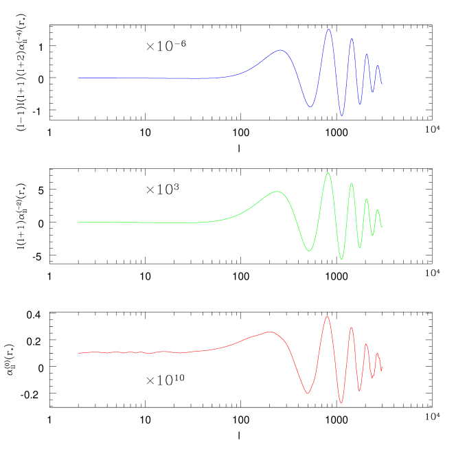
Figure 1: Radial coefficients $\alpha^{(n)}_{\ell}(r)$ [Eq. (94)] at the time of decoupling, $r_{*}$. From top to bottom we plot $(\ell-1)\ell(\ell+1)(\ell+2)\alpha^{(-4)}_{\ell}(r_{*})$, $\ell(\ell+1)\alpha^{(-2)}_{\ell}(r_{*})$, $\alpha^{(0)}_{\ell}(r_{*})$, respectively.

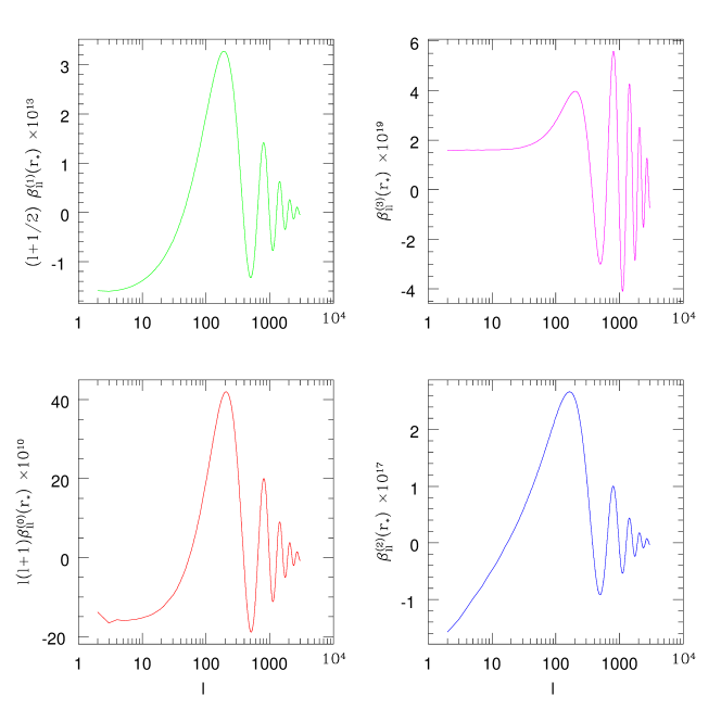
Figure 2: Radial coefficients $\beta^{(n)}_{l}(r)$ [Eq. (95)] at the time of decoupling, $r_{*}$. On the left side, from top to bottom: $(\ell+{1/2})\beta^{(1)}_{\ell\ell}(r_{*})$, $\ell(\ell+1)\beta^{(0)}_{\ell\ell}(r_{*})$. On the right side, from top to bottom: $\beta^{(3)}_{\ell\ell}(r_{*})$, $\beta_{\ell\ell}^{(2)}(r_{*})$.

III.2 Signal-to-noise ratio for WMAP

Even if a significant angular bispectrum was detected in CMB, this would not necessarily mean that it was generated by some primordial mechanism like inflation. There are in fact several foregrounds which can produce non-Gaussianity in CMB anisotropies, such as the Sunyaev-Zel’dovich (SZ) effect, weak lensing, the presence of point sources, and so on. Thus a complete study of detectability of the primary bispectrum needs to include the secondary bispectra generated by the foregrounds, in order to check if the primordial component can be isolated from others.

Having calculated numerically the angle-averaged bispectrum from primary and secondary sources, we evaluate a $\chi^{2}$ statisticks

$$\chi^{2}=\sum_{2\leq\ell_{1}\leq\ell_{2}\leq\ell_{3}}\frac{\left(B_{\ell_{1}\ell_{2}\ell_{3}}^{obs}-\sum_{i}A_{i}B_{\ell_{1}\ell_{2}\ell_{3}}^{(i)}\right)}{\sigma^{2}_{\ell_{1}\ell_{2}\ell_{3}}}\;,$$ (96)

where $B_{\ell_{1}\ell_{2}\ell_{3}}^{obs}$ is the observed bispectrum and $B_{\ell_{1}\ell_{2}\ell_{3}}^{(i)}$ are the theoretically calculated bispectra for different components, denoted by $i$. The variance $\sigma^{2}_{\ell_{1}\ell_{2}\ell_{3}}$ of the bispectrum can be written as sg ; mg

$$\sigma^{2}_{\ell_{1}\ell_{2}\ell_{3}}=\left\langle B_{\ell_{1}\ell_{2}\ell_{3}}^{2}\right\rangle-\left\langle B_{\ell_{1}\ell_{2}\ell_{3}}\right\rangle^{2}\simeq C_{\ell_{1}}C_{\ell_{2}}C_{\ell_{3}}\Delta_{\ell_{1}\ell_{2}\ell_{3}}\;,$$ (97)

where $\Delta_{\ell_{1}\ell_{2}\ell_{3}}$ takes values $1$, $2$, and $6$ when all $\ell$’s are different, two of them are equal and all are the same, respectively. $C_{\ell}$ is the sum of the theoretical CMB angular power-spectrum and the power-spectrum of the detector noise. The last one can be calculated analytically using Ref. knox .

Taking ${\partial\chi^{2}/\partial A_{i}}=0$, the Fisher matrix is given by ks

$$F_{ij}=\sum_{2\leq\ell_{1}\leq\ell_{2}\leq\ell_{3}}\frac{B_{\ell_{1}\ell_{2}\ell_{3}}^{(i)}B_{\ell_{1}\ell_{2}\ell_{3}}^{(j)}}{\sigma^{2}_{\ell_{1}\ell_{2}\ell_{3}}}\;,$$ (98)

and the signal-to-noise ratio $({S/N})_{i}$ for a component $i$ is

$$\left(\frac{S}{N}\right)_{i}=\frac{1}{\sqrt{F_{ii}^{-1}}}\;.$$ (99)

Let us neglect for the moment the non-diagonal components of the Fisher matrix; then, denoting the primordial component by $i=1$, we can give an estimate of the expected signal-to-noise ratio for the primordial non-Gaussian signal without considering foregrounds. It is simply

$$\left(\frac{S}{N}\right)_{1}\sim\sqrt{F_{11}}\;.$$ (100)

We have calculated the approximated signal-to-noise ratio using formula (100) for an experiment with the FWHM beam-size of WMAP ($FWHM=13^{{}^{\prime}}$, $\ell_{\textrm{max}}=500$), assuming different scenarios for the generation of the cosmological perturbations, namely the standard single-field slow roll scenario, the inhomogeneous reheating scenario and the curvaton scenario. The shape of the kernel in all these scenarios is given by Eq. (83) with model-dependent values of the constant $a_{\rm NL}$. According to Ref. komreview , in single-field slow roll inflation $a_{\rm NL}=1$, in the inhomogeneous reheating case $a_{\rm NL}={1/4}$, whereas in the curvaton scenario we have $a_{\rm NL}=({3/4r})-{r/2}$, where $r$ is the relative curvaton contribution to the total energy density at curvaton decay.

Let us now comment on our results, starting from the standard single-field inflation and the inhomogeneous reheating cases. Even though we ignore correlations between the primordial and secondary bispectra, we find, for the standard inflationary scenario, the expected signal-to-noise ratio for WMAP is ${S/N}\simeq 0.10$ and, for the inhomogeneous reheating case, ${S/N}\simeq 0.15$; thus, the primordial non-Gaussianity from these models is below the WMAP detection threshold. As the correlation between the primordial and secondary bispectra would only lower the signal-to-noise ratio for the primordial component, we can conclude that the primordial bispectrum from these scenarios is undetectable with WMAP.

These expectations confirm the ones obtained in the previous work where the non-Gaussian primordial gravitational potential was approximated as $\Phi_{\rm NL}=\Phi_{\rm L}+f_{\rm NL}\Phi_{\rm L}^{2}$ and $f_{\rm NL}$ is a momentum-independent parameter defining the level of predicted non-Gaussianity. In this framework Komatsu and Spergel derived a detection threshold of $f_{\rm NL}=20$ for WMAP and $f_{\rm NL}=5$ for Planck. This suggested that a primordial signal from standard single-field inflation would be undetectable by WMAP as, in this phenomenological approach, $f_{\rm NL}$ was expected to be $\simeq 1$ in the standard scenario ks ; Gangui ; Salopek ; Carroll .

III.3 Challenges of numerical calculations at high $\ell$

Before we study the expected signal-to-noise ratio for the future high-resolution experiments such as Planck, we note that the kind of computation we have described so far is numerically very challenging. Even after parallelizing and optimizing as much as possible, our algorithm (e.g. by implementing analytic approximations for the Wigner coefficients and by minimizing the number of points in the integration samples), the highest $\ell_{\textrm{max}}$ we can reach is $\ell_{\textrm{max}}=500$, corresponding to the angular resolution of the WMAP satellite. We have not been able to go beyond the WMAP resolution, as the CPU time requirement was too demanding. The parallelized version of our algorithm took $6$ hours on $100$ processors to calculate the full bispectrum up to $\ell_{\textrm{max}}=500$. As the CPU time scales roughly as $\ell_{\textrm{max}}^{5}$ it would take about 5 years on the same number of processors to calculate it up to $\ell_{\textrm{max}}=3000$, thus making approximations necessary. On the other hand, extrapolating our results to higher angular resolutions suggests that the primordial non-Gaussian signal could be significant enough to allow detection of the primary signal at $\ell_{max}=3000$ (the angular resolution of the Planck satellite), even in the most standard single-field slow roll inflationary scenario. This will be explained in more detail in the next section.

III.4 Prospects for detecting non-Gaussianity by Planck

Komatsu and Spergel ks pointed out that even an ideal experiment needed $f_{\rm NL}>3$ in order to detect primordial non-Gaussianity. This last statement, when combined with the previous theoretical expectations of the amplitude of non-Gaussianity, $f_{\rm NL}\simeq 1$, implied rather pessimistic prospects for detecting the primordial non-Gaussian signals in standard scenarios of single-field inflation.

However, we stress here that the previous expectation, $f_{\rm NL}\simeq 1$, even though it roughly took into account the effect of the post-inflationary evolution of non-Gaussianity, was not based on the detailed second-order computation of the cosmological perturbations during and after inflation. For this reason, it must be considered only as an order of magnitude estimate, and care must be taken when we study detectability of non-Gaussianity from standard single-field inflation by the future experiments at high angular resolution such as Planck.

Our prediction based on the complete second-order calculation of the primordial gravitational potential shows an encouraging trend which shows that the actual signal-to-noise ratio is larger than the previous prediction with $f_{\rm NL}=1$. Even though it is insufficient to push the primary signal over the detectability threshold of WMAP, it could be big enough to allow detection of the primordial non-Gaussianity signals by Planck.

Figure 3: Values of $f_{\rm NL}^{eff}(\ell_{\rm max})$ (Eq. [102]) in the standard single-field and inhomogeneous reheating scenarios. This parameter, $f^{eff}_{\rm NL}(\ell_{\rm max})$, represents $f_{\rm NL}$ in the usual parametrization of non-Gaussianity to reproduce the same level of non-Gaussianity predicted by our model for a given $\ell_{\rm max}$. For the standard single-field inflation the contribution to non-Gaussianity comes only from the post-inflation non-linear processing of perturbations, which is independent of the inflationary model. Thus the solid line in the plots also represents that part of the non-Gaussian signal which must be present in the CMB anisotropies, regardless of the considered inflationary model. The lower panel shows our results for an experiment with beam size and noise characteristics similar to WMAP. The upper panel shows the same analysis for Planck. We are considering $\ell_{\textrm{max}}=500$, corresponding to the angular resolution of WMAP. A full analysis for Planck would require $\ell_{\textrm{max}}=3000$, which is beyond the current computational power (see Sec III.3).

Let us elaborate on this point. We evaluate the signal-to-noise ratio for $10<\ell_{\textrm{max}}<500$ both in our cases and in the standard $f_{\rm NL}$ parametrization. In the standard parametrization of non-Gaussianity the signal-to-noise ratio can be written as:

$$\left(\frac{S}{N}\right)^{\rm stand}=f_{\rm NL}\sqrt{F^{\rm stand}_{11}(f_{\rm NL}=1)}\;,$$ (101)

where $F^{\rm stand}_{11}(f_{\rm NL}=1)$ is the Fisher matrix of the standard $f_{\rm NL}$ model with $f_{\rm NL}=1$. The idea is as follows: by comparing the actual signal-to-noise ratio predicted from our full calculations, $(S/N)^{\rm full}$, to the standard one, we can estimate $f_{\rm NL}$ that is required to produce the same $(S/N)^{\rm stand}$ in the standard parametrization as $(S/N)^{\rm full}$:

$$f^{eff}_{\rm NL}(\ell_{\rm max})\equiv\frac{\left({S/N}\right)^{\rm full}}{\sqrt{F^{\rm stand}_{11}(f_{\rm NL}=1)}}\;,$$ (102)

which is the $f_{\rm NL}$ that is needed in the usual parametrization of non-Gaussianity to reproduce the same level of non-Gaussianity predicted by our model for a given $\ell_{\rm max}$. This parameter allows us to compare the previous estimates to ours more easily. The results are shown in figure 3, where we consider two experiments with the beam and the noise characteristics similar to WMAP and Planck. Two things are worth noticing. First of all, $f_{\rm NL}^{eff}(\ell_{\rm max})$ is not constant over $\ell_{\rm max}$. Second of all, $f_{\rm NL}^{eff}(\ell_{\rm max}=500)$ is significantly bigger than the previously expected value, $f_{\rm NL}\simeq 1$, though it is still of the same order of magnitude. When we look at the Planck experiment, we also notice that $f_{\rm NL}^{eff}(\ell_{\rm max})$ is monotonically increasing when $\ell_{\rm max}\geq 40$, reaching a value of $f_{\rm NL}^{eff}(\ell_{\rm max}=500)\simeq 4$,which is already very close to the detection threshold $f_{\rm NL}=5$ computed by Komatsu and Spergel ks for the full resolution of Planck. Considering that the angular resolution of the Planck satellite corresponds to $\ell_{\textrm{max}}=3000$, and we stopped our computation at $\ell_{\textrm{max}}=500$, our results suggest that the non-Gaussian signal from standard single-field inflation is likely to be detected by Planck.

In addition to the standard single-field inflation and the inhomogeneous reheating models, we also investigate the curvaton scenario. In this case the value of $a_{\rm NL}$ depends on the parameter $r$, the relative curvaton contribution to the total energy density at curvaton decay, as previously pointed out. We consider different values of $r$, and calculate $f_{\rm NL}^{\rm eff}(\ell_{\rm max})$. Note that the momentum-independent part has been calculated as $f_{\rm NL}=-{5/(4r)}+{5r/6}$ BMR3 . Our results are summarized in table 1. We notice that, for small values of $r$, the parameter $f_{\rm NL}^{eff}(\ell_{\rm max}=500)$ is now smaller than what was expected in the previous predictions (meaning that our signal-to-noise ratio is smaller than what was predicted assuming the standard $f_{\rm NL}$ parametrization), whereas $f_{\rm NL}^{eff}(\ell_{\rm max}=500)>f_{\rm NL}$ for $r\geq 0.5$. Therefore, it is incorrect to conclude that the amplitude of non-Gaussianity is smaller for larger $r$; on the contrary, the signal-to-noise stays nearly the same regardless of $r$.

$\;\;\;\;\mathbf{r}\;\;\;\;$	$\;\;\;\;\;\mathbf{|f_{\rm NL}|}\;\;\;\;\;$	$\;\;\;\;\;\mathbf{f_{\rm NL}^{eff}}\;\;\;\;\;$	$\;\;\;\;\;\mathbf{{S/N}}\;\;\;\;\;$
$0.1$	$12.42$	$8.42$	$0.24$
$0.2$	$6.10$	$2.98$	$0.08$
$0.3$	$3.92$	$2.62$	$0.06$
$0.4$	$2.79$	$2.58$	$0.07$
$0.5$	$2.10$	$2.98$	$0.08$
$0.6$	$1.58$	$3.31$	$0.10$
$0.7$	$1.20$	$3.60$	$0.10$
$0.8$	$0.90$	$3.84$	$0.10$
$0.9$	$0.64$	$4.04$	$0.11$
$1.0$	$0.42$	$4.22$	$0.12$

Table 1: Results for the curvaton model. The first two columns show the value of the relative curvaton contribution to the total energy density at curvaton decay and the predicted values of $f_{\rm NL}$ in the previous parameterization which assumes that $f_{\rm NL}$ is a constant. The last two columns contain the new computation of $f_{\rm NL}^{eff}(\ell_{\rm max}=500)$ (Eq. [102]) and of the signal-to-noise ratio for WMAP.

Before concluding this section, let us stress again that our rough estimate of $f_{\rm NL}^{eff}(\ell_{\rm max})$ and the extrapolation of our results to the angular resolution of the Planck satellite does not allow any conclusive statement about detectability of the primordial non-Gaussian signals generated by the simplest models of inflation. It is important to keep in mind that our $f_{\rm NL}^{eff}(\ell_{\rm max})$ depends on $\ell_{\rm max}$; thus, it is still possible that $f_{\rm NL}^{eff}(\ell_{\rm max})$ might start to decrease for $\ell_{\rm max}>500$ and stay below the detection threshold of Planck at $\ell_{\rm max}=3000$. However, we find an encouraging trend that $f_{\rm NL}^{eff}(\ell_{\rm max})$ increases monotonically for $\ell_{\rm max}\gtrsim 40$. It is certainly worth finding a way to achieve the full numerical computation of the primordial bispectrum (60) at very high multipoles ($\ell_{\textrm{max}}\simeq 3000$). The current algorithm based on the full numerical integration of equation (60) is computationally very expensive, and most likely some approximations must be invoked; one possibility is to implement the flat sky approximation at high $\ell$’s. This will be the topic of a forthcoming publication flatsky .

IV Conclusions

In this paper, we have shown that the full second-order calculations of cosmological perturbations and inflationary dynamics suggest that the realistic form of non-Gaussianity, the kernel $f_{\rm NL}({\mathbf{k}}_{1},{\mathbf{k}}_{2},\mathbf{k_{3}})$, must contain momentum-dependent terms. We have derived the analytic formula for the angle-averaged primary CMB angular bispectrum. This formula allows a more realistic description of non-Gaussian CMB anisotropy, extending the phenomenological model adopted in Ref. ks , where $f_{\rm NL}$ was taken to be a constant. We have developed a numerical code to compute the primary bispectrum and estimated the expected signal-to-noise ratio for detecting primary non-Gaussianity at the WMAP angular resolution. Our results show that, in the framework of standard single-field inflation, the primary non-Gaussian signal cannot be detected by WMAP, as already indicated by the previous analysis. On the other hand, in our complete second-order approach to perturbations during and after inflation, we have found that the previous theoretical expectation, $f_{\rm NL}\simeq 1$, was too pessimistic, and the actual value which defines the CMB bispectrum is much larger. This result implies that the primordial non-Gaussian signals might be detectable by the future Planck mission even in the standard single-field scenarios of inflation. However, using the current numerical algorithm, we have not been able to reach Planck’s angular resolution, $\ell_{\rm max}=3000$, which would require 5 years of CPU time on 100 processors, and our conclusion on the prospect for detecting non-Gaussianity by Planck has to rely on extrapolations from $\ell_{\rm max}=500$. Suitable approximations at high $\ell$’s will be required in the future, in order to make a definitive conclusion on detectability of primordial non-Gaussianity in CMB. Finally, let us comment on statistical methods to measure the bispectrum. Komatsu, Spergel and Wandelt ksw have shown that the direct measurement of all possible configurations of the bispectrum is computationally too expensive, and developed a faster estimator of $f_{\rm NL}$ assuming that $f_{\rm NL}$ is a constant. Recently, Creminelli et al. paolo have extended this method to the case where the dominant signals come from the equilateral configurations, which yields a certain momentum-dependence in $f_{\rm NL}$. Their model (Eq. [14] of paolo ), however, is different from the form of $f_{\rm NL}(\mathbf{k_{1}},\mathbf{k_{2}},\mathbf{k_{3}})$ in equation (83), and thus their estimator cannot be used to measure primordial non-Gaussianity from second-order perturbations. New estimators optimized to our $f_{\rm NL}(\mathbf{k_{1}},\mathbf{k_{2}},\mathbf{k_{3}})$ need to be developed.

References

• (1) D. H. Lyth and A. Riotto, Phys. Rept. 314 (1999) 1.
• (2) C. L. Bennett, et al., Astrophys. J. Suppl. 148 (2003) 1.
• (3) H. V. Peiris, et al., Astrophys. J. Suppl. 148 (2003) 213.
• (4) S. Mollerach, Phys. Rev. D 42 (1990) 313.
• (5) K. Enqvist and M. S. Sloth, Nucl. Phys. B 626 (2002) 395.
• (6) D. H. Lyth and D. Wands, Phys. Lett. B 524 (2002) 5.
• (7) T. Moroi and T. Takahashi, Phys. Lett. B 522 (2001) 215 [Erratum-ibid. B 539 (2002) 303].
• (8) D. H. Lyth, C. Ungarelli and D. Wands, Phys. Rev. D 67 (2003) 023503.
• (9) N. Bartolo, E. Komatsu, S. Matarrese and A. Riotto, Phys. Rept. (2005).
• (10) G. Dvali, A. Gruzinov and M. Zaldarriaga, Phys. Rev. D 69 (2004) 023505; L. A. Kofman, arXiv:astro-ph/0303614.
• (11) E.W. Kolb, A. Riotto and A. Vallinotto, Phys. Rev. D 71 (2005) 043513.
• (12) V. Acquaviva, N. Bartolo, S. Matarrese and A. Riotto, Nucl. Phys. B 667 (2003) 119.
• (13) J. Maldacena, JHEP 0305 (2003) 013.
• (14) N. Bartolo, S. Matarrese and A. Riotto, JHEP 0404 (2004) 006.
• (15) N. Bartolo, S. Matarrese and A. Riotto, Phys. Rev. D 69 (2004) 043503.
• (16) N. Bartolo, S. Matarrese and A. Riotto, JCAP 0401 (2004) 003.
• (17) N. Bartolo, S. Matarrese and A. Riotto, Phys. Rev. Lett.  93 (2004) 231301.
• (18) N. Bartolo, S. Matarrese and A. Riotto, astro-ph/0506410.
• (19) G. I. Rigopoulos, E. P. S. Shellard and B. W. van Tent, astro-ph/0410486; D. H. Lyth and Y. Rodriguez, Phys. Rev. D 71 (2005) 123508; idem astro-ph/0504045.
• (20) E. Komatsu and D. N. Spergel, Phys. Rev. D 63 (2001) 063002.
• (21) E. Komatsu, et al., Astrophys. J. Suppl.  148 (2003) 119.
• (22) D. N. Spergel and D. M. Goldberg, Phys. Rev. D 59 (1999) 103001.
• (23) A. Gangui and J. Martin, Phys. Rev. D 62, 103004 (2000).
• (24) L. Knox, Phys. Rev. D 52, 4307 (1995).
• (25) F. K. Hansen, et al., in preparation
• (26) D. S. Salopek and J. R. Bond, Phys. Rev.  D 42 3936 (1990); ibid. 43 1005 (1991)
• (27) A. Gangui, F. Lucchin, S. Matarrese and S. Mollerach, Astrophys. J. 430 447 (1994)
• (28) T. Pyne and S.M. Carroll, Phys. Rev.  D 53 2920 (1996)
• (29) E. Komatsu, D.N. Spergel and B.D. Wandelt, Astrophys. J., in press (astro-ph/0305189)
• (30) P. Creminelli, A. Nicolis, L. Senatore, M. Tegmark and M. Zaldarriaga, astro-ph/0509029